CDR: Conservative Doubly Robust Learning for Debiased Recommendation

Abstract.

In recommendation systems (RS), user behavior data is observational rather than experimental, resulting in widespread bias in the data. Consequently, tackling bias has emerged as a major challenge in the field of recommendation systems. Recently, Doubly Robust Learning (DR) has gained significant attention due to its remarkable performance and robust properties. However, our experimental findings indicate that existing DR methods are severely impacted by the presence of so-called Poisonous Imputation, where the imputation significantly deviates from the truth and becomes counterproductive.

To address this issue, this work proposes Conservative Doubly Robust strategy (CDR) which filters imputations by scrutinizing their mean and variance. Theoretical analyses show that CDR offers reduced variance and improved tail bounds. In addition, our experimental investigations illustrate that CDR significantly enhances performance and can indeed reduce the frequency of poisonous imputation.

1. Introduction

Enabled by a variety of deep learning techniques, the field of recommendation systems (RS) has seen significant advancements (Zhang et al., 2020; Zhao et al., 2019). Nonetheless, the direct application of these advanced RS models in real-world scenarios is often impeded by the presence of numerous biases. Among these, selection bias is especially prominent, referring to the occurrence that the observed data might not faithfully represent the entirety of user-item pairs (Marlin and Zemel, 2009; Marlin et al., 2012). Selection bias has detrimental effects not only on the accuracy of the recommendations, but it may also foster unfairness and potentially exacerbate the Matthew effect (Zhang et al., 2021; Gao et al., 2022b; Marlin and Zemel, 2009).

A myriad of methods to counter selection bias have been introduced in recent years. These approaches fall primarily into three categories: 1) Generative models (Kim and Choi, 2014; Wang et al., 2020, 2022), which resorts to a causal graph to depict the generative process of observed data and infer user true preference accordingly. However, given the complexity of real-world RS scenarios, accurately constructing a causal graph poses a significant challenge. 2) Inverse Propensity Score (IPS) (Schnabel et al., 2016; Swaminathan and Joachims, 2015), which adjusts the data distribution by reweighing the observed samples. While IPS can theoretically achieve unbiasedness, its performance is highly sensitive to propensity configuration and prone to high variance. 3) Doubly Robust Learning (DR) (Wang et al., 2019; Guo et al., 2021; Dai et al., 2022; Ding et al., 2022), which enhances IPS by incorporating error imputation for all user-item pairs. DR enjoys the doubly robust property where unbiasedness is guaranteed if either the imputed values or propensity scores are accurate.

Encouraged by the promising performance and theoretical advantages of DR, this study opts for the DR approach. However, we highlight a potential limitation of current DR methods — they conduct imputation for all user-item pairs, potentially leading to poisonous imputation. In DR, imputation values rely on the imputation model, which is typically trained on a small set of observed data and extrapolated to the entire user-item pairs. Consequently, it is inevitable for the imputation model to produce inaccurate estimations on certain user-item pairs. Poisonous imputation arises when the imputed values significantly diverge from the truth to such an extent that they negatively impact the debiasing process and could even compromise the model’s performance. Upon examining existing DR methods on real-world datasets, we found that the ratio of poisonous imputation is notably high, often exceeding 35%. Addressing poisonous imputation is thus essential for the effectiveness of a DR method.

A straightforward solution to this issue could be to directly identify and eliminate poisonous imputations. However, this is practically infeasible due to the unavailability of ground-truth labels of user preference for the majority of user-item pairs. To address this challenge, we propose a Conservative Doubly Robust strategy (CDR) that constructs a surrogate filtering protocol by scrutinizing the mean and variance of the imputation value. Theoretical analyses demonstrate our CDR achieves lower variance and better tail bound compared to conventional DR. Remarkably, our solution is model-agnostic and can be easily plug-in existing DR methods. In our experiments, we implemented CDR in four different methods, demonstrating that CDR yields superior recommendation performance and a reduced ratio of poisonous imputation.

To summarize, this work makes the following contributions:

• Exposing the issue of poisonous imputation within existing Doubly Robust methods in Recommendation Systems.

• Proposing a Conservative Doubly Robust strategy (CDR) that mitigates the problem of poisonous imputation through examination of the mean and variance of the imputation value.

• Performing rigorous theoretical analyses and conducting extensive empirical experiments to validate the effectiveness of CDR.

2. Analyses over Doubly Robust Learning

In this section, we first formulate the task of recommendation debiasing (Sec. 2.1), and then present some background of doubly robust learning (Sec. 2.2). Finally, we identify the issue of poisonous imputation on existing DR methods (Sec. 2.3).

2.1. Task Formulation

Suppose we have a recommender system composed of a user set $\mathcal{U}$ and an item set $\mathcal{I}$. Let $\mathcal{D=U\times I}$ denote the set of all user-item pairs. Further, let $r_{ui}\in\mathbb{R}$ be the ground-truth label (e.g., rating) for a user-item pair $(u,i)$, indicating how the user likes the item; and $\hat{r}_{ui}$ be the corresponding predicted label from a recommendation model. The collected historical rating data can be notated as a set $\mathbf{R}^{o}=\{r_{ui}|o_{ui}=1\}$, where $o_{ui}$ denotes whether the rating of a user-item pair $(u,i)$ is observed. The goal of a RS is to accurately predict user preference and accordingly identify items that align with users’ tastes. The ideal loss for training a recommendation model can be formulated as follow:

(1) $$\mathcal{L}_{ideal}\ =\ \mid\mathcal{D}\mid^{-1}\sum_{(u,i)\in\mathcal{D}}e_{ui}$$

Where $e_{ui}$ denotes the prediction error between $r_{ui}$ and $\hat{r}_{ui}$, e.g., $e_{ui}=|r_{ui}-\hat{r}_{ui}|^{2}$ with RMSE loss or $e_{ui}=-r_{ui}\log(\hat{r}_{ui})-(1-r_{ui})\log(1-\hat{r}_{ui})$ with BCE loss. However, only a small portion of $r_{ui}$ is observed in RS, rendering the ideal loss non-computable. Moreover, the challenge is further accentuated by the presence of selection bias, as the observed data might not faithfully represent the entirety of user-item pairs. For instance, samples with higher ratings are more likely to be observed (Marlin and Zemel, 2009). Utilizing a naive estimator that calculates directly on the observed data with $\mathcal{L}_{naive}=\mid\mathcal{D}\mid^{-1}\sum_{(u,i)\in\mathcal{D}}o_{ui}e_{ui}$ would yield a biased estimation (Schnabel et al., 2016). Hence, the exploration for a suitable surrogate loss towards unbiased estimation of the ideal loss is ongoing.

2.2. Existing Estimators

Now we review two typical estimators for addressing selection bias.

Inverse Propensity Score Estimator (IPS) (Schnabel et al., 2016). The IPS estimator aims to adjust the training distribution by reweighing the observed instances as:

(2) $$\mathcal{L}_{IPS}\ =\ \mid\mathcal{D}\mid^{-1}\sum_{(u,i)\in\mathcal{D}}\frac{o_{ui}e_{ui}}{\hat{p}_{ui}}$$

where $\hat{p}_{ui}$ is an estimation of the propensity score $p_{ui}=\mathbb{P}(o_{ui}=1)$. The bias and variance of IPS estimator can be written as:

(3) $$\begin{split}Bias[\mathcal{L}_{IPS}]&=\mathbb{|}E_{o}[\mathcal{L}_{IPS}]-\mathcal{L}_{Ideal}|\\ &=\mid\mathcal{D}\mid^{-1}\lvert\sum_{(ui)\in\mathcal{D}}\frac{(p_{ui}-\hat{p}_{ui})}{\hat{p}_{ui}}{e_{ui}}\rvert\\ Var[\mathcal{L}_{IPS}]&=\mathbb{E}_{o}[(\mathcal{L}_{IPS}-\mathbb{E}_{o}[\mathcal{L}_{IPS}])^{2}]\\ &=\mid\mathcal{D}\mid^{-2}\sum_{(u,i)\in\mathcal{D}}\frac{p_{ui}(1-p_{ui})}{\hat{p}_{ui}^{2}}{{e}_{ui}^{2}}\end{split}$$

Once the $\hat{p}_{ui}$ reaches its ideal value (i.e., $\hat{p}_{ui}=p_{ui}$), the IPS estimator could provide an unbiased estimation of the ideal loss (i.e., $\mathbb{E}_{o}[\mathcal{L}_{IPS}]=\mathcal{L}_{Ideal}$).

Doubly Robust Estimator (DR) (Wang et al., 2019). DR augments IPS by introducing the error imputation with the following loss:

(4) $$\mathcal{L}_{DR}\ =\ \mid\mathcal{D}\mid^{-1}\sum_{(u,i)\in\mathcal{D}}(\hat{e}_{ui}+\frac{o_{ui}(e_{ui}-\hat{e}_{ui})}{\hat{p}_{ui}})$$

where $\hat{e}_{ui}$ represents the imputed error, derived from a specific imputation model that strives to fit the predicted error. Recent work (Guo et al., 2021) has established the bias and variance of DR as follow:

(5) $$\begin{split}Bias[\mathcal{L}_{DR}]&=\mid\mathcal{D}\mid^{-1}\lvert\sum_{(u,i)\in\mathcal{D}}\frac{(p_{ui}-\hat{p}_{ui})}{\hat{p}_{ui}}{(e_{ui}-\hat{e}_{ui})}\rvert\\ Var[\mathcal{L}_{DR}]&=\mid\mathcal{D}\mid^{-2}\sum_{(u,i)\in\mathcal{D}}\frac{p_{ui}(1-p_{ui})}{\hat{p}_{ui}^{2}}{(\hat{e}_{ui}-e_{ui})^{2}}\end{split}$$

As can be seen, DR change the bias term for each $(u,i)$ from $\frac{(p_{ui}-\hat{p}_{ui})}{\hat{p}_{ui}}{e_{ui}}$ in IPS to $\frac{(p_{ui}-\hat{p}_{ui})}{\hat{p}_{ui}}{(e_{ui}-\hat{e}_{ui})}$ and the variance from $\frac{p_{ui}(1-p_{ui})}{\hat{p}_{ui}^{2}}{{e}_{ui}^{2}}$ to $\frac{p_{ui}(1-p_{ui})}{\hat{p}_{ui}^{2}}{(\hat{e}_{ui}-e_{ui})^{2}}$. DR enjoys the doubly robust property that if either $\hat{p}_{ui}=p_{ui}$ or $e_{ui}=\hat{e}_{ui}$ holds, $\mathcal{L}_{DR}$ could be an unbiased estimator (i.e., $Bias[\mathcal{L}_{DR}]=0$). This advantageous property typically results in DR being less biased than IPS in practice, empirically leading to superior performance.

2.3. Limitation of DR

	Coat	Yahoo	KuaiRand
DR-JL	45.9%	41.9%	38.8%
MRDR	48.1%	43.1%	41.2%
DR-BIAS	44.1%	40.4%	39.2%
TDR	42.3%	36.2%	36.3%

Table 1. The proportion of ”poisonous imputation” in three different datasets using four typical DR methods.

From the eq.(5), we can conclude that the accuracy of imputation $\hat{e}_{ui}$ is of highly importance — both the bias and variance term are correlated with $|\hat{e}_{ui}-e_{ui}|$. Indeed, if the imputed error $\hat{e}_{ui}$ diverges significantly from the predicted error $e_{ui}$ such that $|\hat{e}_{ui}-e_{ui}|>e_{ui}$, the imputation $\hat{e}_{ui}$ becomes counterproductive. Particularly, imputing $\hat{e}_{ui}$ for the user-item pair $(u,i)$ results in increased bias and variance, rather than reduced. We denote this phenomenon as poisonous imputation:

Definition 2.1 (Poisonous Imputation).

For any user-item pair $(u,i)$, the imputation $\hat{e}_{ui}$ is considered as a poisonous imputation if $|\hat{e}_{ui}-e_{ui}|>e_{ui}$.

In practical RS, given that the imputation model is typically trained on a limited set of observed data and generalized to the entire user-item pairs, poisonous imputation is frequently encountered. To provide empirical evidence for this point, we conducted an empirical analysis on four representative DR methods (DR-JL (Wang et al., 2019), MRDR (Guo et al., 2021), DR-BIAS (Dai et al., 2022), and TDR (Li et al., 2023a)) across three real-world debiasing datasets (YahooR3, Coat, and KuaiRand). These DR methods were finely trained on the biased training data, after which $e_{ui}$ and $\hat{e}_{ui}$ were calculated for the user-item pairs in the test data where ground-truth ratings are accessible. The proportion of poisonous imputation is reported in Table 1. Surprisingly, the ratio of poisonous imputation is considerably high, often exceeding 35% across all datasets and baseline models. It is noteworthy that even though DR generally exhibits superior performance over IPS, a substantial amount of poisonous imputation still exists. The issue of poisonous imputation is particularly severe, thereby warranting attention and resolution.

3. METHODOLOGY

In this section, we first introduce the proposed conservative doubly robust strategy, and then conduct theoretical analyses to validate its merits.

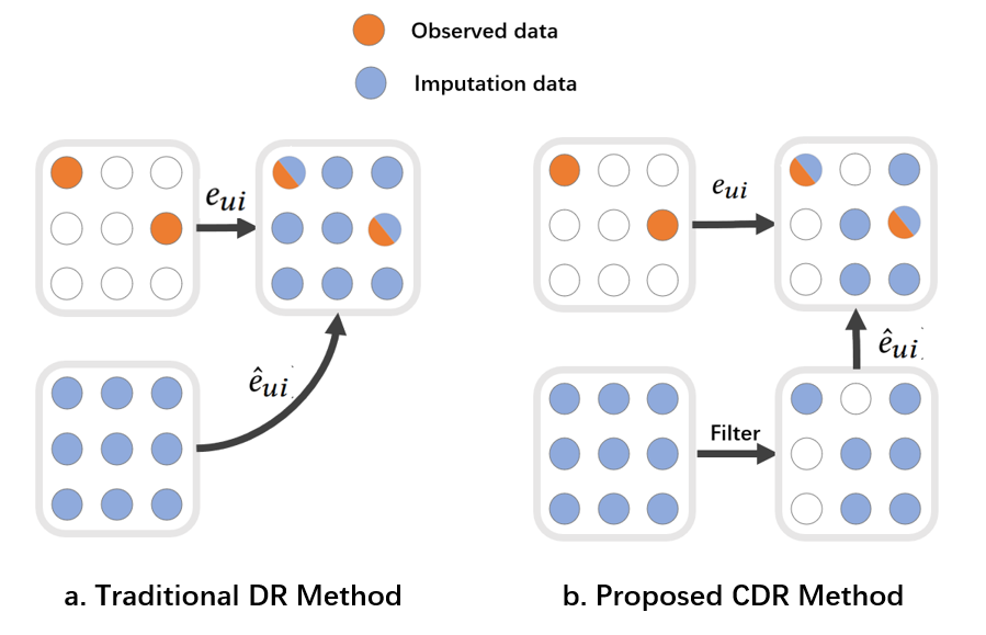
Figure 1. Illustration of how our CDR improves the traditional DR methods — leveraging a filter protocol to remove the poisonous imputation that may hurt debiasing.

3.1. Conservative Doubly Robust Learning

Considering the widespread occurrence of poisonous imputation, we contend that performing imputation blindly on all user-item pairs, as is customary with current methods, may not be the optimal strategy. Instead, it would be more effective to adopt a conservative and adaptive imputation approach that focuses on user-item pairs which confer benefits while excluding those leading to poisonous imputation. As previously discussed, the ideal filtering protocol involves comparing $|\hat{e}_{ui}-e_{ui}|$ with $e_{ui}$. If $|\hat{e}_{ui}-e_{ui}|<e_{ui}$, the imputation should be retained as it could potentially reduce both variance and bias; if not, it implies a poisonous imputation which should be discarded. However, this approach is impractical as the ground-truth labels are typically inaccessible in real-world scenarios and $e_{ui}$ cannot be calculated. As such, an alternative filtering protocol is necessary.

Towards this end, we propose a Conservative Doubly Robust (CDR) strategy in this work that filters imputation by examining the mean and variance of $\hat{e}_{ui}$. The foundation of CDR is based on the following important lemma:

Lemma 1.

Given that $\hat{e}_{ui}$ and $e_{ui}$ are independently drawn from two Gaussian distributions $\mathcal{N}(\hat{\mu}_{ui},\hat{\sigma}^{2}_{ui})$ and $\mathcal{N}(\mu_{ui},\sigma^{2}_{ui})$, where $\hat{\mu}_{ui}$, $\mu_{ui}$, $\hat{\sigma}_{ui}$, $\sigma_{ui}$ are bounded with $|\hat{\mu}_{ui}-\mu_{ui}|\leq\varepsilon_{\mu}$, $|\hat{\sigma}_{ui}^{2}-\sigma_{ui}^{2}|\leq\varepsilon_{\sigma}^{2}$, $2\varepsilon_{\mu}\leq\hat{\mu}_{ui}$, $m_{\mu}\leq\hat{\mu}_{ui}\leq M_{\mu}$ and $m_{\sigma}\leq\hat{\sigma}_{ui}\leq M_{\sigma}$, for any confidence level $\rho$ ($0\leq\rho\leq 1$), the condition $\mathbb{P}(|\hat{e}_{ui}-e_{ui}|<e_{ui})\geq\rho$ holds if

(6) $$\frac{{{{\hat{\sigma}}_{ui}}}}{{{{\hat{\mu}}_{ui}}}}<{\bigg{(}\sqrt{5}{\Phi^{-1}}(\rho)+\frac{{2{M_{\mu}}{\varepsilon_{\sigma}}}}{{{m_{\sigma}}(\sqrt{5}{m_{\sigma}}+2{\varepsilon_{\sigma}})}}+\frac{{2\sqrt{5}{\varepsilon_{\mu}}}}{{\sqrt{5}{m_{\sigma}}+2{\varepsilon_{\sigma}}}}\bigg{)}^{-1}}$$

where $\Phi^{-1}(.)$ denotes the inverse of CDR of the standard normal distribution.

The proof of the lemma is included in the appendix A. This lemma indicates that through the formulation of a distribution hypothesis for $\hat{e}_{ui}$ and $e_{ui}$, the evaluation of poisonous imputation can be reframed as a scrutiny of the mean and variance of $\hat{e}_{ui}$. The hypothesis presented in the lemma is practical. On one hand, we hypothesize that the distribution of $\hat{e}_{ui}$ approximates that of $e_{ui}$ (i.e., $|\hat{\mu}_{ui}-\mu_{ui}|\leq\varepsilon_{\mu}$, $|\hat{\sigma}_{ui}^{2}-\sigma_{ui}^{2}|\leq\varepsilon_{\sigma}^{2}$, $2\varepsilon_{\mu}\leq\hat{\mu}_{ui}$), a supposition that naturally follows since the imputation model endeavors to fit $e_{ui}$. On the other hand, we opt to employ the Gaussian distribution for analysis. This choice is informed by its widespread usage in statistical inference, as well as its standing as a second-order Taylor approximation of any distribution. While more complex distributions might yield more precise results, e.g., considering higher-order moments, the analytical complexity and computational burden would significantly increase. Our empirical findings indicate that the Gaussian distribution suffices to deliver superior performance.

In fact, our proposed filtering protocol (inequality (6)) is intuitively appealing due to three observations: 1) A larger value of $\hat{\sigma}_{ui}$ makes the preservation of the imputation less likely. This is consistent with the understanding that a higher variance implies a less reliable prediction, thus making it more susceptible to discarding. 2) A larger value of $\hat{\mu}_{ui}$ makes the preservation of the imputation more likely. This can be rationalized by the notion that if the error $e_{ui}$ is large, the imputation is safer as it is more difficult to exceed $2e_{ui}$. 3) Larger values of $\varepsilon_{\mu}$ and $\varepsilon_{\sigma}$ increase the likelihood of filtering the imputation. Larger values for these parameters suggest a more significant distributional gap between $e_{ui}$ and $\hat{e}_{ui}$, thereby necessitating more conservative filtering.

Instantiation of CDR. CDR can be incorporated into various DR methods by leveraging an additional filtering protocol. This protocol consists of two steps:

1) Estimation of $\hat{\mu}_{ui},\hat{\sigma}_{ui}$: We utilize the Monte Carlo Dropout method (Gal and Ghahramani, 2016) for estimating the mean and variance of the imputation, owing to its generalization and easy implementation. Specifically, we apply dropout 10 times on the imputation model (i.e., randomly omitting 50% of the dimensions of embeddings) and then calculate the mean and variance of $\hat{e}_{ui}$ from the dropout model. To ensure a fair comparison, we should note that dropout is only employed during the calculation of $\hat{\mu}_{ui},\hat{\sigma}_{ui}$, and not during the training of the imputation model.

2) Filtering based on the condition $\frac{\hat{\sigma}_{ui}}{\hat{\mu}_{ui}}<\eta$: Note that the right-hand side of inequality (6) involves complex computation and five parameters. To simplify our implementation, we re-parameterize the right-hand side of the inequation as a hyperparameter $\eta$. This parameter $\eta$ can be interpreted as an adjusted threshold that directly modulates the strictness of the filtering process.

With the above filtering protocol, the CDR estimator can be formulated as:

(7) $$\mathcal{L}_{CDR}=|{\mathcal{D}}{|^{-1}}\sum\limits_{(u,i)\in{\mathcal{D}}}{(\frac{{{o_{ui}}{e_{ui}}}}{{{{\hat{p}}_{ui}}}}+{\gamma_{ui}}{{\hat{e}}_{ui}}(1-\frac{o_{ui}}{{{{\hat{p}}_{ui}}}}))}$$

where $\gamma_{ui}\in\{0,1\}$ indicate whether the imputation $\hat{e}_{ui}$ is retained.

3.2. Theoretical Analyses

In order to elucidate the advantages of the Conservative Doubly Robust (CDR) strategy, we present the following lemma:

Lemma 2.

Given the imputed errors $\hat{e}_{ui}$, estimated propensity scores $\hat{p}_{ui}$, and the retention of the imputation $\gamma_{ui}$, the bias and variance of the CDR estimator can be expressed as follows:

(8) $$\begin{split}Bias[\mathcal{L}_{CDR}]&=\frac{1}{|{\mathcal{D}}|}\lvert\!\!\!\sum\limits_{(u,i)\in{\mathcal{D}}}\!\!\!{\frac{{({p_{ui}}\!-\!{{\hat{p}}_{ui}})}}{{{{\hat{p}}_{ui}}}}({\gamma_{ui}}}({e_{ui}}\!-\!{{\hat{e}}_{ui}})\!+\!(1\!-\!{\gamma_{ui}}){e_{ui}})\rvert\\ Var[\mathcal{L}_{CDR}]&=\frac{1}{|{\mathcal{D}}|^{2}}\!\!\!\sum\limits_{(u,i)\in{\mathcal{D}}}\!\!\!{\frac{{{p_{ui}}(1\!-\!{p_{ui}})}}{{\hat{p}_{ui}^{2}}}}({\gamma_{ui}}{({{\hat{e}}_{ui}}\!-\!{e_{ui}})^{2}}\!+\!(1\!-\!{\gamma_{ui}})e_{ui}^{2})\end{split}$$

With probability $1-\kappa$, the deviation of the CDR estimator from its expectation has the following tail bound:

(9) $$|\mathcal{L}_{CDR}\!-\!\mathbb{E}_{o}[\mathcal{L}_{CDR}]|\!\leq\!\sqrt{\frac{{\log\left({\frac{2}{\kappa}}\right)}}{{2|{\mathcal{D}}{|^{2}}}}\!\!\!\sum\limits_{u,i\in{\mathcal{D}}}\!\!\!{({\gamma_{ui}}\frac{{{{({e_{ui}}\!-\!{{\hat{e}}_{ui}})}^{2}}}}{{\hat{p}_{ui}^{2}}}\!+\!(1\!-\!{\gamma_{ui}})\frac{{e_{ui}^{2}}}{{\hat{p}_{ui}^{2}}})}}$$

The proof is presented in appendix B. CDR can be understood as an integration of IPS and DR . If $|\hat{e}_{ui}-e_{ui}|>e_{ui}$, CDR will filter out the poisonous imputation and regress to IPS, as IPS demonstrates superior bias and variance properties compared to DR . Otherwise, CDR will retain the imputation, benefiting from the merits of DR . Indeed, CDR has the following advantages:

Corollary 3.1.

Under the condition of Lemma 1 and ${\varepsilon_{\mu}}\ll{\hat{\mu}_{ui}},\varepsilon_{\mu}^{2}\ll\hat{\sigma}_{ui}^{2}$, with a proper filtering threshold $\eta$, CDR enjoys better variance and tail bound than IPS and DR.

The proof is presented in appendix C. This corollary substantiates the superiority of CDR, thereby yielding better recommendation performance. We will empirical validate it in the following section.

Table 2. Performance comparison between our CDR with other baselines on three real-world datasets. The best result in that column is bolded and the runner-up is underlined. We incorporate CDR into four baseline models and report the relative improvements gained by employing CDR compared to the respective baseline.

Method	Coat			Yahoo			KuaiRand
	AUC	NDCG@5	Recall@5	AUC	NDCG@5	Recall@5	AUC	NDCG@5	Recall@5
MF	0.7053	0.6025	0.6173	0.6720	0.6252	0.7155	0.5432	0.2932	0.2905
IPS	0.7144	0.6173	0.6267	0.6785	0.6345	0.7214	0.5446	0.2987	0.2987
CVIB	0.7230	0.6278	0.6347	0.6811	0.6482	0.7229	0.5512	0.3099	0.3027
INV	0.7416	0.6394	0.6542	0.6767	0.6443	0.7251	0.5465	0.3081	0.3013
TDR	0.7388	0.6378	0.6525	0.6789	0.6436	0.7269	0.5523	0.3088	0.3026
EIB	0.7225	0.6288	0.6382	0.6844	0.6427	0.7241	0.5456	0.3010	0.2938
EIB+CDR	0.7509	0.6533	0.6608	0.6909	0.6549	0.7310	0.5510	0.3087	0.2975
impv%	+3.93%	+3.90%	+3.54%	+0.95%	+1.90%	+0.95%	+0.99%	+2.56%	+1.26%
DR-JL	0.7286	0.6271	0.6355	0.6834	0.6474	0.7236	0.5485	0.2967	0.2924
DR+CDR	0.7502	0.6557	0.6658	0.6881	0.6558	0.7307	0.5540	0.3153	0.3045
impv%	+2.96%	+4.56%	+4.77%	+0.69%	+1.31%	+0.98%	+1.00%	+6.27%	+4.14%
MRDR	0.7319	0.6317	0.6447	0.6829	0.6484	0.7243	0.5503	0.3041	0.2949
MRDR+CDR	0.7508	0.6520	0.6587	0.6879	0.6571	0.7311	0.5547	0.3167	0.3078
impv%	+2.58%	+3.21%	+2.17%	+0.73%	+1.34%	+0.94%	+0.80%	+4.14%	+4.48%
DR-BIAS	0.7424	0.6408	0.6578	0.6860	0.6486	0.7269	0.5478	0.3024	0.2952
DR-BIAS+CDR	0.7513	0.6567	0.6678	0.6912	0.6565	0.7323	0.5533	0.3098	0.3048
impv%	+1.20%	+2.48%	+1.52%	+0.76%	+1.22%	+0.74%	+1.00%	+2.45%	+3.25%

4. Experiments

In this section, we designed experiments to test the performance of the proposed method on three real-world datasets. Our aim was to answer the following four research questions:

• Does the proposed CDR improve the debiasing performance?

• Does CDR indeed reduce the ratio of poisonous imputation in DR?

• How does the hyperparameter $\eta$ (filtering threshold) affect debiasing performance?

• Does CDR incur much more computational time?

4.1. Experimental Setup

Datasets. To evaluate the performance of debiasing methods on real-world datasets, The ground-truth unbiased data are necessary. We closely refer to previous studies(Schnabel et al., 2016; Wang et al., 2019; Guo et al., 2021; Gao et al., 2022a), and use the following three benchmark datasets: Coat, Yahoo!R3 and KuaiRand-Pure. All three datasets consist of a biased dataset, collected from normal user interactions, and an unbiased dataset collected from random logging strategy. Specifically, Coat includes 6,960 biased ratings and 4,640 unbiased ratings from 290 users for 300 items; Yahoo!R3 comprises 54,000 unbiased ratings and 311,704 biased ratings from 15,400 users for 1,000 items; while KuaiRand includes 7,583 videos and 27,285 users, containing 1,436,609 biased data and 1,186,059 unbiased data. Following recent work (Chen et al., 2021), we regard the biased data as training set, and utilize the unbiased data for model validation (10%) and evaluation (90%). Also, the ratings are binarized with threshold 3. That is, the observed rating value larger than 3 is labeled as positive, otherwise negative.

Baselines. We validate the effectiveness of CDR on four baselines including three benchmark DR methods and one classical baseline just based on imputation:

• EIB(Steck, 2013): the classical baseline that relies on data imputation for tackling selection bias.

• DR-JL(Wang et al., 2019): the basic doubly robust learning strategy that employs both propensity and imputation for recommendation debiasing. In DR-JL, the imputation is learned by minimizing the error deviation on observed data.

• MRDR(Guo et al., 2021): the method improves DR-JL by considering the variance reduction for learning imputation model.

• DR-BIAS(Dai et al., 2022): the novel strategy that learns imputation with balancing the variance and bias.

We also compare the methods with:

• Base Model: the basic recommendation model without employing any debiasing strategy.

• IPS(Schnabel et al., 2016): the strategy that addresses bias via weighing the observed data with the inverse of the propensity.

• INV(Wang et al., 2022): the state-of-the-art debiasing method that leverages causal graph to disentangle the invariant preference and variant factors from the observed data.

• TDR(Li et al., 2023a): the state-of-the-art DR method that learns imputation with a parameterized imputation model and a non-parameter strategy. Here we do not implement CDR in TDR due to its high complexity. Nevertheless, our experiments show that even CDR is plug-in the basic DR-JL, it could outperform TDR.

Also, for fair comparison, we closely refer to recent work (Chen et al., 2021) and take the widely used Matrix Factorization (MF) (Koren et al., 2009) as the base recommendation model.

Metrics. We employed three concurrent metrics, namely, Area Under the Curve (AUC), Recall (Recall@5) and Normalized Discounted Cumulative Gain (NDCG@5) to assess debiasing performance. NDCG@K evaluates the quality of recommendations by taking into account the importance of each item’s position, based on discounted gains.

(10) $$\begin{split}DCG_{u}@K&=\sum_{(u,i)\in\mathcal{D}_{test}}\frac{I(\hat{z}_{u,i}<=K)}{log(\hat{z}_{u,i}+1)}\\ NDCG@K&=\frac{1}{\mid\mathcal{U}\mid}\sum_{u\in\mathcal{U}}\frac{DCG_{u}@K}{IDCG_{u}@K}\end{split}$$

where IDCG represents the ideal DCG, $\mathcal{D}_{test}$ denotes the test data, $\hat{z}_{u,i}$ represents the position of item $i$ within the recommended rank for user $u$.

Recall@K measures the number of recommended items that are likely to be interacted with by the user within top $K$ items.

(11) $$\begin{split}Recall_{u}@K&=\frac{\sum_{(u,i)\in\mathcal{D}_{test}I(\hat{z}_{u,i}<=k)}}{\mid\mathcal{D}^{u}_{test}\mid}\\ Recall@K&=\frac{1}{\mid\mathcal{U}\mid}\sum_{u\in\mathcal{U}}Recall_{u}@K\end{split}$$

where $\mathcal{D}^{u}_{test}$ indicates all ratings of the user $u$ in dataset $\mathcal{D}_{test}$.

Experimental details. Our experiments were conducted on PyTorch, utilizing Adam as the optimizer. We fine-tuned the learning rate within {0.005, 0.01, 0.05, 0.1}, weight decay within {1e - 5, 5e - 5, 1e - 4, 5e - 4, 1e - 3, 5e - 3, 1e - 2}, threshold’s parameter $\eta$ within {0.1, 0.5, 1, 3, 5, 7, 10, 50}, and batch size within {128, 256, 512, 1024, 2048} for Coat , {1024, 2048, 4096, 8192, 16384} for Yahoo!R3 and { 2048, 4096, 8192, 16384, 32768} for KuaiRand. The hyperparameters of all the baselines are finely tuned in our experiments or referred to the orignal paper. The code is available at $https://github.com/CrazyDumpling/CDR\_CIKM2023$.

Table 3. Empirical runtime (s) comparison on Coat, Yahoo and KuaiRand datasets.

Datasets	MF	IPS	EIB	DR-JL	MRDR	DR-bias	EIB+CDR	DR-JL+CDR	MRDR+CDR	DR-bias+CDR
Coat	33.87	36.72	112.80	136.72	131.69	138.23	135.62	147.31	153.28	149.31
Yahoo	59.34	68.91	542.35	632.79	687.34	678.28	643.21	732.13	706.39	714.32
KuaiRand	834.13	1034.24	5018.23	6390.25	6246.36	6421.56	7124.54	6893.49	7154.83	7245.71

4.2. Performance Comparison (RQ1)

Table 2 presents performance comparison of our with other Baselines. We draw the following observations:

1) CDR consistently boosts the recommendation performance on four baselines and three benchmark datasets. Especially in KuaiRand, the improvement is impressive — achieving average 0.95%, 3.86%, 3.28% improvement in terms of AUC, NDCG and Recall respectively. This result validates that our filtering protocol is effective, which could indeed filter the harmful imputation. We will further validate this point in the next experiment.

2) By comparing CDR with other baselines, we can find the best performance always achieved by CDR. CDR is simple but achieves SOTA performance.

4.3. Study on the Poisonous Imputation (RQ2)

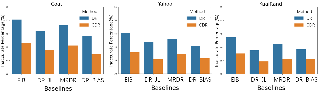
Figure 2. The percentage(%) of ”poisonous imputation” in three different datasets using the original EIB, DR-JL, MRDR and DR-BIAS methods, as well as the improved methods with integrating CDR.

To further validate the effectiveness of CDR, we conducted empirical study on the ratio of the poisonous imputation. We finely trained compared methods on the biased training data, and then compared $|e_{ui}-\hat{e}_{ui}|$ with $e_{ui}$ for the user-item pairs in the test data where ground-truth ratings are accessible. The results are presented in Figure 2.

As can be seen, CDR consistently has lower ratio of poisonous imputation than its corresponding baselines over three datasets. This result clearly validate that the proposed filter is reasonable and can remove a certain ratio of poisonous imputation. As such, CDR achieves better debiasing performance than DR.

4.4. Effect of Hyperparameter $\eta$ (RQ3)

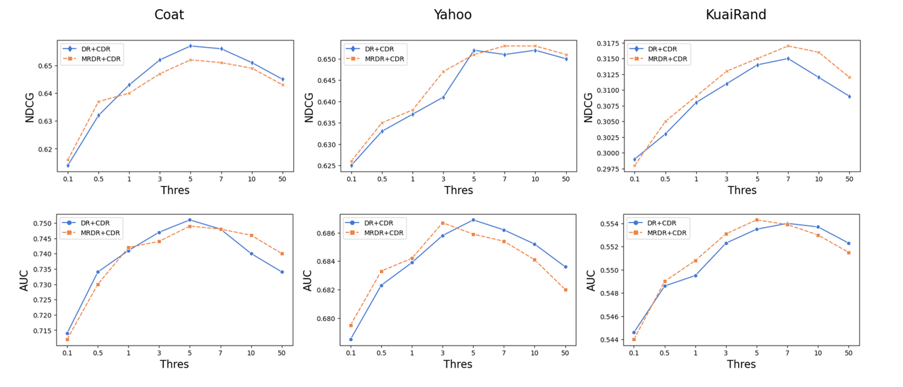
Figure 3. Recommendation performance of CDR with varying threshold $\eta$ on three datasets.

The hyperparameter $\eta$ serves as an adjusted threshold that directly modulates the strictness of the filtering process. Thus, exploring model performance w.r.t. $\eta$ could help us to better understand the nature of CDR. In theoretical terms, when $\eta$ approaches 0, this method is equivalent to IPS; when $\eta$ approaches infinity, this method is equivalent to the DR approach. The performance with varying $\eta$ is presented in Figure 3.

As can be seen, with $\eta$ increasing, the performance will become better first. The reason is that the larger $\eta$ would bring more imputation. As the threshold $\eta$ is relatively low, the injected imputation is usually confidence, yielding performance improvement. However, when $\eta$ surpasses a certain value, the performance becomes worse with further increase of $\eta$. This can be interpreted by the more inaccurate imputation is injected. poisonous imputation occurs which would deteriorate model performance. Consequently, there exists a trade-off on the selection of $\eta$. Only when $\eta$ is set to a proper value, the model achieves the optimal performance.

4.5. Running Time Comparison (RQ4)

Additionally, we conducted experiments on the efficiency of CDR compared with other baselines on three datasets: Coat, Yahoo, and KuaiRand. As shown in the table 3, despite CDR introduces multiply times dropout for evaluating the mean and variance of the imputation, it does not incur much more computation burden. The reason can be attributed to the two factors: 1) The calculation of the mean and variance only involves forward propagation, without requiring the time-consuming backward propagation; 2) CDR would filter a certain ratio of the imputation, which make the samples in training reduced, leading to acceleration when training the recommendation model.

5. Related Work

In this section, we review the most related work from the following two perspectives.

Debiasing in Recommendation. Bias is a critical issue in recommendation systems as it not only hurt recommendation accuracy, but can limit the diversity of recommended items and reinforce unfairness (Chen et al., 2023a; Wu et al., 2022; Gao et al., 2023). There are various sources of bias found in RS data, such as selection bias (Marlin and Zemel, 2009; Marlin et al., 2012; Chen et al., 2018), exposure bias (Liu et al., 2020; Chen et al., 2019, 2020), conformity bias (Liu et al., 2016; Wang and Wang, 2014), position bias (Joachims et al., 2017, 2007) and popularity bias (Abdollahpouri and Mansoury, 2020; Wei et al., 2021; Chen et al., 2023b; Zhao et al., 2022). To address this issue, the academic community has probed into a multitude of methodologies to rectify the bias in recommendation systems. Given the focus of this study on selection bias, we primarily concentrate our review on the latest advancements in tackling this particular bias. For a more comprehensive understanding, we recommend readers to refer to the bird’s-eye-view survey (Chen et al., 2023a) for additional details.

Recent work on selection bias can be mainly categorized into three types:

1) Generative Models, which resorts to a causal graph to depict the generative process of observed data and infer user true preference accordingly. The most representative methods are (Chen et al., 2018; Marlin and Zemel, 2009; Kim and Choi, 2014; Hernández-Lobato et al., 2014), which jointly model the which rating value the user gives and which items the user select to rate. More recently, some researchers utilize the causal graph to disentangle the invariant preference from other variant factors (Wang et al., 2022, 2020) thereby enabling the recommendation to depend on the reliable invariant user preferences.

2) Inverse Propensity Score, which adjusts the data distribution by reweighing the observed samples with the inverse of the propensity. Once the propensity reaches the ideal value, IPS could provide an unbiased estimation of the ideal loss. Recent studies (Schnabel et al., 2016; Wang et al., 2021) have introduced a range of methodologies to learn propensities including calculating from item popularity, fitting a model to the observation, or computing from a limited set of unbiased data.

3) Doubly Robust Learning, which enhances IPS by incorporating error imputation for all user-item pairs. DR enjoys the doubly robust property where unbiasedness is guaranteed if either the imputed values or propensity scores are accurate. The merit of DR relies on the accuracy of the imputation model. Thus, various learning strategies are proposed by recent work. For example, DR-JL (Wang et al., 2019) jointly learn the recommendation model and imputation model from the observed data, while the imputation model is optimized to minimize the error deviation on observed data; AutoDebias (Chen et al., 2021) leverages the unbiased data to supervise the learning of the imputation via meta-learning; MRDR (Guo et al., 2021) considers the variance reduction in learning imputation model; DR-BIAS (Dai et al., 2022) learns the imputation with balancing the variance and bias. More recently, some researchers consider to further boost the instability and generalization of DR with leveraging the stable regularizer (Li et al., 2023b) and non-parameter imputation module (Li et al., 2023a). While these approaches offer promising solutions for debiasing recommendation, they all impute the error for all user-item pairs and may suffer from the issue of poisonous imputation.

Uncertainty Estimation. Utilization of probabilistic models to assess and control uncertainty (a.k.a. variance), has found broad applications across numerous fields. This approach is usually characterized by probabilistic inference, which allows for continuous updating of beliefs about model parameters. Uncertainty estimation have found extensive use in diverse domains including machine learning (Loquercio et al., 2020), natural language processing, signal processing and clustering (Zhou et al., 2022). A prevalent approach incorporates Bayesian neural networks (Blundell et al., 2015; Kingma et al., 2015; Molchanov et al., 2017; Louizos and Welling, 2017), providing a flexible and efficient framework to encapsulate uncertainty within neural network predictions. Another line for uncertainty estimation is the MC-dropout technique (Gal and Ghahramani, 2016; Gal et al., 2017; Owen, 2013), which simply perform multiple dropout and estimate the uncertainty (variance) via different models after dropout. Recent work has connected MC-dropout with Bayesian inference and shows that MC-dropout serves as a form of variational Bayesian inference with leveraging a spike and slab variational distribution. Besides, methods like Kronecker Factored Approximation (KFAC) (Ritter et al., 2018) and Markov Chain Monte Carlo (MCMC) (Mandt et al., 2017; Welling and Teh, 2011) have been deployed to propagate uncertainties in intricate models. In this work, we simply choose MC-dropout to estimate the uncertainty of the imputation model, while it can be easily replaced by other advanced technologies.

6. Conclusion and Future Work

This study identifies the issue of poisonous imputation in recent Doubly Robust (DR) methods – these methods indiscriminately perform imputation on all user-item pairs, including those with poisonous imputations that significantly deviate from the truth and negatively impact the debiasing performance. To counter this problem, we introduce a novel Conservative Doubly Robust (CDR) strategy that filters out poisonous imputation by examining the mean and variance of the imputation value. Both theoretical analyses and empirical experiments have been conducted to validate the superiority of our proposal.

For future research, it would be compelling to explore more advanced filtering protocols. Our CDR strategy is based on the assumption on Gaussian distribution of the imputation, which may not be high accurate. Employing sophisticated techniques such as Dynamic Graph neural network (Bei et al., 2023), Generative Adversarial Networks (GAN) (Creswell et al., 2018) or diffusion models (Croitoru et al., 2023) to account for more flexible distributions could be promising. Moreover, as per Table 3, DR methods typically exhibit much more computational burden compared to basic models. Therefore, investigating methods to accelerate DR presents another promising direction for future work.

Appendix A Proof of Lemma 1

Note that the errors $e_{ui}$ and $\hat{e}_{ui}$ are often defined as positive values, e.g., in the context of BCE loss or RMSE loss. Consequently, we can deduce $P(|{e_{ui}}-{{\hat{e}}_{ui}}|<{e_{ui}})=P({{\hat{e}}_{ui}}-2{e_{ui}}<0)$. Moreover, even in cases where the positive of $e_{ui}$ and $\hat{e}_{ui}$ is not maintained for certain losses, we still have the relations $P(|{e_{ui}}-{{\hat{e}}_{ui}}|<{e_{ui}})\geq P({{\hat{e}}_{ui}}-2{e_{ui}}<0)$. Thus, we would like to take the $P({{\hat{e}}_{ui}}-2{e_{ui}}<0)$ for analyses.

For convenient, let $g={{\hat{e}}_{ui}}-2{e_{ui}}$. Considering ${{\hat{e}}_{ui}}$ and ${e_{ui}}$ are two independent variables subject to gaussian distribution $\mathcal{N}(\hat{\mu}_{ui},\hat{\sigma}^{2}_{ui})$ and $\mathcal{N}(\mu_{ui},\sigma^{2}_{ui})$ respectively, we can easily write the distribution of $g$ as $\mathcal{N}(\hat{\mu}_{ui}-2\mu_{ui},\hat{\sigma}^{2}_{ui}+4\sigma^{2}_{ui})$ (Bishop and Nasrabadi, 2006). Let $z$ be a variable from standard gaussian distribution. We further have:

(12) $$\begin{split}P(g<0)&=P(\frac{{g-({{\hat{\mu}}_{ui}}-2{\mu_{ui}})}}{{\sqrt{\hat{\sigma}_{ui}^{2}+4\sigma_{ui}^{2}}}}<-\frac{{{{\hat{\mu}}_{ui}}-2{\mu_{ui}}}}{{\sqrt{\hat{\sigma}_{ui}^{2}+4\sigma_{ui}^{2}}}})\\ &\geq P(z<-\frac{{{{\hat{\mu}}_{ui}}-2({{\hat{\mu}}_{ui}}-{\varepsilon_{\mu}})}}{{\sqrt{\hat{\sigma}_{ui}^{2}+4(\hat{\sigma}_{ui}^{2}+\varepsilon_{\mu}^{2})}}})\\ &=P(z<\frac{{{{\hat{\mu}}_{ui}}-2{\varepsilon_{\mu}}}}{{\sqrt{5\hat{\sigma}_{ui}^{2}+4\varepsilon_{\mu}^{2}}}})\end{split}$$

where the inequality holds, as $\hat{\mu}_{ui}$, $\mu_{ui}$, $\hat{\sigma}_{ui}$, $\sigma_{ui}$ are bounded with $|\hat{\mu}_{ui}-\mu_{ui}|\leq\varepsilon_{\mu}$, $|\hat{\sigma}_{ui}^{2}-\sigma_{ui}^{2}|\leq\varepsilon_{\sigma}^{2}$, $2\varepsilon_{\mu}\leq\hat{\mu}_{ui}$. And when ${\mu_{ui}}={{\hat{\mu}}_{ui}}-{\varepsilon_{\mu}},\sigma_{ui}^{2}=\hat{\sigma}_{ui}^{2}+\varepsilon_{\mu}^{2}$, the right-hand side achieves minimum. Eq.(12) further has the following lower bound:

(13) $$\begin{split}&P(z<\frac{{{{\hat{\mu}}_{ui}}-2{\varepsilon_{\mu}}}}{{\sqrt{5\hat{\sigma}_{ui}^{2}+4\varepsilon_{\sigma}^{2}}}})\\ &\mathop{\geq}\limits_{1}P(z<\frac{{{{\hat{\mu}}_{ui}}-2{\varepsilon_{\mu}}}}{{\sqrt{5}{{\hat{\sigma}}_{ui}}+2{\varepsilon_{\sigma}}}})\\ &=P(z<\frac{{{{\hat{\mu}}_{ui}}}}{{\sqrt{5}{{\hat{\sigma}}_{ui}}}}-(\frac{{2{{\hat{\mu}}_{ui}}{\varepsilon_{\sigma}}}}{{\sqrt{5}{{\hat{\sigma}}_{ui}}(\sqrt{5}{{\hat{\sigma}}_{ui}}+2{\varepsilon_{\sigma}})}}+\frac{{2{\varepsilon_{\mu}}}}{{\sqrt{5}{{\hat{\sigma}}_{ui}}+2{\varepsilon_{\sigma}}}}))\\ &\mathop{\geq}\limits_{2}P(z<\frac{{{{\hat{\mu}}_{ui}}}}{{\sqrt{5}{{\hat{\sigma}}_{ui}}}}-(\frac{{2{M_{\mu}}{\varepsilon_{\sigma}}}}{{{\sqrt{5}m_{\sigma}}(\sqrt{5}{m_{\sigma}}+2{\varepsilon_{\sigma}})}}+\frac{{2{\varepsilon_{\mu}}}}{{\sqrt{5}{m_{\sigma}}+2{\varepsilon_{\sigma}}}}))\end{split}$$

where the first inequaility holds due to the fact that $\sqrt{5}{{\hat{\sigma}}_{ui}}+2{\varepsilon_{\sigma}}\geq\sqrt{5\hat{\sigma}_{ui}^{2}+4\varepsilon_{\sigma}^{2}}$, while the second inequaility holds since ${{{\hat{\mu}}_{ui}}}$ is upper-bounded by ${{M_{\mu}}}$ and ${{{\hat{\sigma}}_{ui}}}$ is lower-bounded by ${{m_{\sigma}}}$.

If we let:

(14) $$\frac{{{{\hat{\sigma}}_{ui}}}}{{{{\hat{\mu}}_{ui}}}}<{\bigg{(}\sqrt{5}{\Phi^{-1}}(\rho)+\frac{{2{M_{\mu}}{\varepsilon_{\sigma}}}}{{{m_{\sigma}}(\sqrt{5}{m_{\sigma}}+2{\varepsilon_{\sigma}})}}+\frac{{2\sqrt{5}{\varepsilon_{\mu}}}}{{\sqrt{5}{m_{\sigma}}+2{\varepsilon_{\sigma}}}}\bigg{)}^{-1}}$$

We can find the following inequaility holds:

(15) $$P(z<\frac{{{{\hat{\mu}}_{ui}}}}{{\sqrt{5}{{\hat{\sigma}}_{ui}}}}-(\frac{{2{M_{\mu}}{\varepsilon_{\sigma}}}}{{{m_{\sigma}}(\sqrt{5}{m_{\sigma}}+2{\varepsilon_{\sigma}})}}+\frac{{2{\varepsilon_{\mu}}}}{{\sqrt{5}{m_{\sigma}}+2{\varepsilon_{\sigma}}}}))\geq\rho$$

Thus, we have $\mathbb{P}(|\hat{e}_{ui}-e_{ui}|<e_{ui})\geq\rho$. The lemma gets proof.

Appendix B Proof of Lemma 2

The bias and variance of CDR can be easily obtained based on the following equations:

(16) $$\begin{split}Bias[\mathcal{L}_{CDR}]&=\mathbb{|}E_{o}[\mathcal{L}_{CDR}]-\mathcal{L}_{Ideal}|\\ &=\frac{1}{|{\mathcal{D}}|}\lvert\!\!\!\sum\limits_{(u,i)\in{\mathcal{D}}}\!\!\!{\frac{{({p_{ui}}\!-\!{{\hat{p}}_{ui}})}}{{{{\hat{p}}_{ui}}}}({\gamma_{ui}}}({e_{ui}}\!-\!{{\hat{e}}_{ui}})\!+\!(1\!-\!{\gamma_{ui}}){e_{ui}})\rvert\\ Var[\mathcal{L}_{CDR}]&=\mathbb{E}_{o}[(\mathcal{L}_{CDR}-\mathbb{E}_{o}[\mathcal{L}_{CDR}])^{2}]\\ &=\frac{1}{|{\mathcal{D}}|^{2}}\!\!\!\sum\limits_{(u,i)\in{\mathcal{D}}}\!\!\!{\frac{{{p_{ui}}(1\!-\!{p_{ui}})}}{{\hat{p}_{ui}^{2}}}}({\gamma_{ui}}{({{\hat{e}}_{ui}}\!-\!{e_{ui}})^{2}}\!+\!(1\!-\!{\gamma_{ui}})e_{ui}^{2})\end{split}$$

The proof of tail bound refers to (Wang et al., 2019) but replaces the $\mathcal{L}_{DR}$ with $\mathcal{L}_{CDR}$. We first let ${l_{ui}}=\frac{{{o_{ui}}{e_{ui}}}}{{{{\hat{p}}_{ui}}}}+{\gamma_{ui}}{{\hat{e}}_{ui}}(1-\frac{1}{{{{\hat{p}}_{ui}}}})$. Note that ${{o_{ui}}}$ is an bernoulli variable and thus the variable $l_{ui}$ takes the value in the interval $[{\gamma_{ui}}{{\hat{e}}_{ui}},\frac{{{e_{ui}}}}{{{{\hat{p}}_{ui}}}}+{\gamma_{ui}}{{\hat{e}}_{ui}}(1-\frac{1}{{{{\hat{p}}_{ui}}}})]$ of size $s_{ui}=(1-{\gamma_{ui}})\frac{{{e_{ui}}}}{{{{\hat{p}}_{ui}}}}+{\gamma_{ui}}\frac{{{e_{ui}}-{{\hat{e}}_{ui}}}}{{{{\hat{p}}_{ui}}}}$. Considering the $o_{ui}$ are independent for different $(u,i)$, Hoeffding inequality (Mohri et al., 2018) can be employed with:

(17) $$P(|\sum\limits_{u,i}{{l_{u,i}}}-{\mathbb{E}_{o}}[{\sum\limits_{u,i}{{l_{ui}}}}]|\geq|\,\mathcal{D}|\epsilon)\leq 2\exp({\frac{{-2|\mathcal{D}|^{2}\epsilon^{2}}}{{\sum\limits_{u,i}{s_{ui}^{2}}}}})$$

Set the right-hand side of the inequality to $\kappa$ and then we can get the lemma 2.

Appendix C Proof of Corollary 3.1

Here we primarily concentrate on demonstrating that CDR outperforms IPS in terms of variance and tail bound. A similar proof process can be applied to DR. Setting $\rho_{0}=0.6$ allows us to derive a set of effective imputations $S=\{(u,i)|P(|{e_{ui}}-{{\hat{e}}_{ui}}|<{e_{ui}})\geq\rho_{0}\}$. If $S=\emptyset$, then CDR regresses to IPS, at least performing equivalently to IPS. Otherwise, it is always possible to identify a user-item pair $(u^{*},i^{*})$ that has the largest $\frac{{{{\hat{\mu}}_{ui}}}}{{{{\hat{\sigma}}_{ui}}}}$ among $S$. We can define $\rho=\Phi(\frac{{{{\hat{\mu}}_{ui}}}}{{\sqrt{5}{{\hat{\sigma}}_{ui}}}}-(\frac{{2{M_{\mu}}{\varepsilon_{\sigma}}}}{{{\sqrt{5}m_{\sigma}}(\sqrt{5}{m_{\sigma}}+2{\varepsilon_{\sigma}})}}+\frac{{2{\varepsilon_{\mu}}}}{{\sqrt{5}{m_{\sigma}}+2{\varepsilon_{\sigma}}}}))-eps$, under the condition that only the imputation with the highest $\frac{{{{\hat{\mu}}_{ui}}}}{{{{\hat{\sigma}}_{ui}}}}$ is preserved, where $eps$ denotes a sufficiently small positive value. Taking into account the continuous values of ${{{{\hat{\sigma}}_{ui}}}},{{{{\hat{\mu}}_{ui}}}}$, the probability of two imputations sharing the exact same value is negligible. Hence, only the imputation for the pair $(u^{*},i^{*})$ is preserved.

To compare the variance and tail bounds between CDR and IPS, we can identify that the key difference pertains to the pair $(u^{*},i^{*})$. Here CDR utilizes $(\hat{e}_{ui}-e_{ui})^{2}$ while IPS utilizes $e_{ui}^{2}$. As the relation $|{e_{ui}}-{{\hat{e}}_{ui}}|<{e_{ui}}$ holds for $(u^{*},i^{*})$ with at least $\rho$ probability, and considering $\rho>\rho_{0}$, we can conclude that CDR achieves better variance and tail bound compared to DR.

References

- (1)
- Abdollahpouri and Mansoury (2020) Himan Abdollahpouri and Masoud Mansoury. 2020. Multi-sided exposure bias in recommendation. arXiv preprint arXiv:2006.15772 (2020).
- Bei et al. (2023) Yuanchen Bei, Hao Xu, Sheng Zhou, Huixuan Chi, Mengdi Zhang, Zhao Li, and Jiajun Bu. 2023. CPDG: A Contrastive Pre-Training Method for Dynamic Graph Neural Networks. arXiv preprint arXiv:2307.02813 (2023).
- Bishop and Nasrabadi (2006) Christopher M Bishop and Nasser M Nasrabadi. 2006. Pattern recognition and machine learning. Vol. 4. Springer.
- Blundell et al. (2015) Charles Blundell, Julien Cornebise, Koray Kavukcuoglu, and Daan Wierstra. 2015. Weight uncertainty in neural network. In International conference on machine learning. PMLR, 1613–1622.
- Chen et al. (2021) Jiawei Chen, Hande Dong, Yang Qiu, Xiangnan He, Xin Xin, Liang Chen, Guli Lin, and Keping Yang. 2021. Autodebias: Learning to debias for recommendation. In Proceedings of the 44th International ACM SIGIR Conference on Research and Development in Information Retrieval. 21–30.
- Chen et al. (2023a) Jiawei Chen, Hande Dong, Xiang Wang, Fuli Feng, Meng Wang, and Xiangnan He. 2023a. Bias and debias in recommender system: A survey and future directions. ACM Transactions on Information Systems 41, 3 (2023), 1–39.
- Chen et al. (2018) Jiawei Chen, Can Wang, Martin Ester, Qihao Shi, Yan Feng, and Chun Chen. 2018. Social recommendation with missing not at random data. In 2018 IEEE International Conference on Data Mining (ICDM). IEEE, 29–38.
- Chen et al. (2020) Jiawei Chen, Can Wang, Sheng Zhou, Qihao Shi, Jingbang Chen, Yan Feng, and Chun Chen. 2020. Fast adaptively weighted matrix factorization for recommendation with implicit feedback. In Proceedings of the AAAI Conference on artificial intelligence, Vol. 34. 3470–3477.
- Chen et al. (2019) Jiawei Chen, Can Wang, Sheng Zhou, Qihao Shi, Yan Feng, and Chun Chen. 2019. Samwalker: Social recommendation with informative sampling strategy. In The World Wide Web Conference. 228–239.
- Chen et al. (2023b) Jiawei Chen, Junkang Wu, Jiancan Wu, Xuezhi Cao, Sheng Zhou, and Xiangnan He. 2023b. Adap-: Adaptively Modulating Embedding Magnitude for Recommendation. In Proceedings of the ACM Web Conference 2023. 1085–1096.
- Creswell et al. (2018) Antonia Creswell, Tom White, Vincent Dumoulin, Kai Arulkumaran, Biswa Sengupta, and Anil A Bharath. 2018. Generative adversarial networks: An overview. IEEE signal processing magazine 35, 1 (2018), 53–65.
- Croitoru et al. (2023) Florinel-Alin Croitoru, Vlad Hondru, Radu Tudor Ionescu, and Mubarak Shah. 2023. Diffusion models in vision: A survey. IEEE Transactions on Pattern Analysis and Machine Intelligence (2023).
- Dai et al. (2022) Quanyu Dai, Haoxuan Li, Peng Wu, Zhenhua Dong, Xiao-Hua Zhou, Rui Zhang, Rui Zhang, and Jie Sun. 2022. A generalized doubly robust learning framework for debiasing post-click conversion rate prediction. In Proceedings of the 28th ACM SIGKDD Conference on Knowledge Discovery and Data Mining. 252–262.
- Ding et al. (2022) Sihao Ding, Peng Wu, Fuli Feng, Yitong Wang, Xiangnan He, Yong Liao, and Yongdong Zhang. 2022. Addressing unmeasured confounder for recommendation with sensitivity analysis. In Proceedings of the 28th ACM SIGKDD Conference on Knowledge Discovery and Data Mining. 305–315.
- Gal and Ghahramani (2016) Yarin Gal and Zoubin Ghahramani. 2016. Dropout as a bayesian approximation: Representing model uncertainty in deep learning. In international conference on machine learning. PMLR, 1050–1059.
- Gal et al. (2017) Yarin Gal, Jiri Hron, and Alex Kendall. 2017. Concrete dropout. Advances in neural information processing systems 30 (2017).
- Gao et al. (2023) Chongming Gao, Kexin Huang, Jiawei Chen, Yuan Zhang, Biao Li, Peng Jiang, Shiqi Wang, Zhong Zhang, and Xiangnan He. 2023. Alleviating Matthew Effect of Offline Reinforcement Learning in Interactive Recommendation. arXiv preprint arXiv:2307.04571 (2023).
- Gao et al. (2022a) Chongming Gao, Shijun Li, Yuan Zhang, Jiawei Chen, Biao Li, Wenqiang Lei, Peng Jiang, and Xiangnan He. 2022a. KuaiRand: An Unbiased Sequential Recommendation Dataset with Randomly Exposed Videos. In Proceedings of the 31st ACM International Conference on Information & Knowledge Management. 3953–3957.
- Gao et al. (2022b) Chongming Gao, Shiqi Wang, Shijun Li, Jiawei Chen, Xiangnan He, Wenqiang Lei, Biao Li, Yuan Zhang, and Peng Jiang. 2022b. CIRS: Bursting filter bubbles by counterfactual interactive recommender system. ACM Transactions on Information Systems (2022).
- Guo et al. (2021) Siyuan Guo, Lixin Zou, Yiding Liu, Wenwen Ye, Suqi Cheng, Shuaiqiang Wang, Hechang Chen, Dawei Yin, and Yi Chang. 2021. Enhanced doubly robust learning for debiasing post-click conversion rate estimation. In Proceedings of the 44th International ACM SIGIR Conference on Research and Development in Information Retrieval. 275–284.
- Hernández-Lobato et al. (2014) José Miguel Hernández-Lobato, Neil Houlsby, and Zoubin Ghahramani. 2014. Probabilistic matrix factorization with non-random missing data. In International conference on machine learning. PMLR, 1512–1520.
- Joachims et al. (2017) Thorsten Joachims, Laura Granka, Bing Pan, Helene Hembrooke, and Geri Gay. 2017. Accurately interpreting clickthrough data as implicit feedback. In Acm Sigir Forum, Vol. 51. Acm New York, NY, USA, 4–11.
- Joachims et al. (2007) Thorsten Joachims, Laura Granka, Bing Pan, Helene Hembrooke, Filip Radlinski, and Geri Gay. 2007. Evaluating the accuracy of implicit feedback from clicks and query reformulations in web search. ACM Transactions on Information Systems (TOIS) 25, 2 (2007), 7–es.
- Kim and Choi (2014) Yong-Deok Kim and Seungjin Choi. 2014. Bayesian binomial mixture model for collaborative prediction with non-random missing data. In Proceedings of the 8th ACM Conference on Recommender systems. 201–208.
- Kingma et al. (2015) Durk P Kingma, Tim Salimans, and Max Welling. 2015. Variational dropout and the local reparameterization trick. Advances in neural information processing systems 28 (2015).
- Koren et al. (2009) Yehuda Koren, Robert Bell, and Chris Volinsky. 2009. Matrix factorization techniques for recommender systems. Computer 42, 8 (2009), 30–37.
- Li et al. (2023a) Haoxuan Li, Yan Lyu, Chunyuan Zheng, and Peng Wu. 2023a. TDR-CL: Targeted Doubly Robust Collaborative Learning for Debiased Recommendations. In The Eleventh International Conference on Learning Representations.
- Li et al. (2023b) Haoxuan Li, Chunyuan Zheng, and Peng Wu. 2023b. StableDR: Stabilized Doubly Robust Learning for Recommendation on Data Missing Not at Random. In The Eleventh International Conference on Learning Representations.
- Liu et al. (2020) Dugang Liu, Pengxiang Cheng, Zhenhua Dong, Xiuqiang He, Weike Pan, and Zhong Ming. 2020. A general knowledge distillation framework for counterfactual recommendation via uniform data. In Proceedings of the 43rd International ACM SIGIR Conference on Research and Development in Information Retrieval. 831–840.
- Liu et al. (2016) Yiming Liu, Xuezhi Cao, and Yong Yu. 2016. Are you influenced by others when rating? Improve rating prediction by conformity modeling. In Proceedings of the 10th ACM conference on recommender systems. 269–272.
- Loquercio et al. (2020) Antonio Loquercio, Mattia Segu, and Davide Scaramuzza. 2020. A general framework for uncertainty estimation in deep learning. IEEE Robotics and Automation Letters 5, 2 (2020), 3153–3160.
- Louizos and Welling (2017) Christos Louizos and Max Welling. 2017. Multiplicative normalizing flows for variational bayesian neural networks. In International Conference on Machine Learning. PMLR, 2218–2227.
- Mandt et al. (2017) S. Mandt, MD Hoffman, and D. M. Blei. 2017. Stochastic Gradient Descent as Approximate Bayesian Inference. Journal of Machine Learning Research 18 (2017).
- Marlin et al. (2012) Benjamin Marlin, Richard S Zemel, Sam Roweis, and Malcolm Slaney. 2012. Collaborative filtering and the missing at random assumption. arXiv preprint arXiv:1206.5267 (2012).
- Marlin and Zemel (2009) Benjamin M Marlin and Richard S Zemel. 2009. Collaborative prediction and ranking with non-random missing data. In Proceedings of the third ACM conference on Recommender systems. 5–12.
- Mohri et al. (2018) Mehryar Mohri, Afshin Rostamizadeh, and Ameet Talwalkar. 2018. Foundations of machine learning. MIT press.
- Molchanov et al. (2017) Dmitry Molchanov, Arsenii Ashukha, and Dmitry Vetrov. 2017. Variational dropout sparsifies deep neural networks. In International Conference on Machine Learning. PMLR, 2498–2507.
- Owen (2013) Art B. Owen. 2013. Monte Carlo theory, methods and examples.
- Ritter et al. (2018) H. Ritter, A. Botev, and D. Barber. 2018. A Scalable Laplace Approximation for Neural Networks. In 6th International Conference on Learning Representations (ICLR 2018).
- Schnabel et al. (2016) Tobias Schnabel, Adith Swaminathan, Ashudeep Singh, Navin Chandak, and Thorsten Joachims. 2016. Recommendations as treatments: Debiasing learning and evaluation. In international conference on machine learning. PMLR, 1670–1679.
- Steck (2013) Harald Steck. 2013. Evaluation of recommendations: rating-prediction and ranking. In Proceedings of the 7th ACM conference on Recommender systems. 213–220.
- Swaminathan and Joachims (2015) Adith Swaminathan and Thorsten Joachims. 2015. The self-normalized estimator for counterfactual learning. advances in neural information processing systems 28 (2015).
- Wang and Wang (2014) Ting Wang and Dashun Wang. 2014. Why Amazon’s ratings might mislead you: The story of herding effects. Big data 2, 4 (2014), 196–204.
- Wang et al. (2019) Xiaojie Wang, Rui Zhang, Yu Sun, and Jianzhong Qi. 2019. Doubly robust joint learning for recommendation on data missing not at random. In International Conference on Machine Learning. PMLR, 6638–6647.
- Wang et al. (2021) Xiaojie Wang, Rui Zhang, Yu Sun, and Jianzhong Qi. 2021. Combating selection biases in recommender systems with a few unbiased ratings. In Proceedings of the 14th ACM International Conference on Web Search and Data Mining. 427–435.
- Wang et al. (2020) Zifeng Wang, Xi Chen, Rui Wen, Shao-Lun Huang, Ercan Kuruoglu, and Yefeng Zheng. 2020. Information theoretic counterfactual learning from missing-not-at-random feedback. Advances in Neural Information Processing Systems 33 (2020), 1854–1864.
- Wang et al. (2022) Zimu Wang, Yue He, Jiashuo Liu, Wenchao Zou, Philip S Yu, and Peng Cui. 2022. Invariant Preference Learning for General Debiasing in Recommendation. In Proceedings of the 28th ACM SIGKDD Conference on Knowledge Discovery and Data Mining. 1969–1978.
- Wei et al. (2021) Tianxin Wei, Fuli Feng, Jiawei Chen, Ziwei Wu, Jinfeng Yi, and Xiangnan He. 2021. Model-agnostic counterfactual reasoning for eliminating popularity bias in recommender system. In Proceedings of the 27th ACM SIGKDD Conference on Knowledge Discovery & Data Mining. 1791–1800.
- Welling and Teh (2011) M. Welling and Y. W. Teh. 2011. Bayesian Learning via Stochastic Gradient Langevin Dynamics. In International Conference on International Conference on Machine Learning.
- Wu et al. (2022) Peng Wu, Haoxuan Li, Yuhao Deng, Wenjie Hu, Quanyu Dai, Zhenhua Dong, Jie Sun, Rui Zhang, and Xiao-Hua Zhou. 2022. On the opportunity of causal learning in recommendation systems: Foundation, estimation, prediction and challenges. In Proceedings of the International Joint Conference on Artificial Intelligence, Vienna, Austria. 23–29.
- Zhang et al. (2020) Yongfeng Zhang, Xu Chen, et al. 2020. Explainable recommendation: A survey and new perspectives. Foundations and Trends® in Information Retrieval 14, 1 (2020), 1–101.
- Zhang et al. (2021) Yang Zhang, Fuli Feng, Xiangnan He, Tianxin Wei, Chonggang Song, Guohui Ling, and Yongdong Zhang. 2021. Causal intervention for leveraging popularity bias in recommendation. In Proceedings of the 44th International ACM SIGIR Conference on Research and Development in Information Retrieval. 11–20.
- Zhao et al. (2019) Xiangyu Zhao, Long Xia, Jiliang Tang, and Dawei Yin. 2019. ” Deep reinforcement learning for search, recommendation, and online advertising: a survey” by Xiangyu Zhao, Long Xia, Jiliang Tang, and Dawei Yin with Martin Vesely as coordinator. ACM Sigweb Newsletter Spring (2019), 1–15.
- Zhao et al. (2022) Zihao Zhao, Jiawei Chen, Sheng Zhou, Xiangnan He, Xuezhi Cao, Fuzheng Zhang, and Wei Wu. 2022. Popularity bias is not always evil: Disentangling benign and harmful bias for recommendation. IEEE Transactions on Knowledge and Data Engineering (2022).
- Zhou et al. (2022) Sheng Zhou, Hongjia Xu, Zhuonan Zheng, Jiawei Chen, Jiajun Bu, Jia Wu, Xin Wang, Wenwu Zhu, Martin Ester, et al. 2022. A comprehensive survey on deep clustering: Taxonomy, challenges, and future directions. arXiv preprint arXiv:2206.07579 (2022).