Detecting Galaxy Tidal Features Using Self-Supervised Representation Learning

Abstract

Low surface brightness substructures around galaxies, known as tidal features, are a valuable tool in the detection of past or ongoing galaxy mergers, and their properties can answer questions about the progenitor galaxies involved in the interactions. The assembly of current tidal feature samples is primarily achieved using visual classification, making it difficult to construct large samples and draw accurate and statistically robust conclusions about the galaxy evolution process. With upcoming large optical imaging surveys such as the Vera C. Rubin Observatory’s Legacy Survey of Space and Time (LSST), predicted to observe billions of galaxies, it is imperative that we refine our methods of detecting and classifying samples of merging galaxies. This paper presents promising results from a self-supervised machine learning model, trained on data from the Ultradeep layer of the Hyper Suprime-Cam Subaru Strategic Program optical imaging survey, designed to automate the detection of tidal features. We find that self-supervised models are capable of detecting tidal features, and that our model outperforms previous automated tidal feature detection methods, including a fully supervised model. An earlier method achieved 76% completeness for 22% contamination, while our model achieves considerably higher (96%) completeness for the same level of contamination. We emphasise a number of advantages of self-supervised models over fully supervised models including maintaining excellent performance when using only 50 labelled examples for training, and the ability to perform similarity searches using a single example of a galaxy with tidal features.

1 Introduction

The currently accepted model of the Universe, known as the Lambda Cold Dark Matter ($\Lambda$CDM) Cosmological Model, postulates that galaxies evolve through a process which is referred to as the ‘hierarchical merger model’, wherein the growth of the universe’s highest-mass galaxies is dominated by merging with lower-mass galaxies (e.g. Lacey & Cole 1994; Cole et al. 2000; Robotham et al. 2014; Martin et al. 2018). During the merging process, the extreme gravitational forces involved cause stellar material to be pulled out from the galaxies, forming diffuse non-uniform regions of stars in the outskirts of the galaxies, known as tidal features (e.g. Toomre & Toomre 1972). Examples of these features from the optical Hyper Suprime-Cam Subaru Strategic Program (HSC-SSP; Aihara et al. 2018) are shown in Figure 1. These tidal features contain information about the merging history of the galaxy, and can thus be used to study the galaxy evolution process. Using tidal features to detect merging galaxies has a number of advantages over other methods such as spectroscopically detected galaxy close pairs. Not only do they remain observable significantly longer than close pairs (a few Gyr compared to $\sim$ 600 Myr; Lotz et al. 2011; Hendel & Johnston 2015; Huang & Fan 2022) but they can also be used to identify mergers where a companion galaxy has already been ripped apart or is too low mass to be detected spectroscopically. Hence, using tidal features to study galaxy evolution can provide important observational confirmation on the contribution of low-mass galaxies to the merging process (e.g. Johnston et al. 2008).

In order to draw accurate and statistically robust conclusions about this evolution process, we require a large sample of galaxies exhibiting tidal features. This is difficult to achieve due to the extremely low surface brightness of tidal features, which can easily reach $\mu_{r}\geq$ 27 mag $\rm{arcsec}^{-2}$. The limiting surface brightness of wide-field optical astronomical surveys often do not reach these depths and as a consequence, many tidal features will not be identified simply because the features are not visible. This not only causes tidal feature incidence measures to be too low, but also increases the work required and number of images that need to be classified to assemble a sample with a significant number of galaxies with tidal features. With the next generation of wide-field optical imaging surveys reaching new limiting depths, such as the Vera C Rubin Observatory’s Legacy Survey of Space and Time (LSST; Ivezić et al. 2019) which is predicted to reach $\mu_{r}\sim$ 30.3 mag $\rm{arcsec}^{-2}$ (Martin et al., 2022), assembling a statistically significant sample of galaxies with tidal features is becoming more feasible. One challenge associated with surveys like LSST, due to commence in 2025 and run for 10 years, is the amount of data predicted to be released, with LSST predicted to output over 500 petabytes of imaging data including billions of galaxies (Ivezić et al., 2019). Current tidal feature detection and classification is primarily achieved through visual identification (e.g. Tal et al. 2009; Sheen et al. 2012; Atkinson et al. 2013; Hood et al. 2018; Bílek et al. 2020; Martin et al. 2022), but billions of galaxies are virtually impossible to classify visually by humans, even using large community based projects such as Galaxy Zoo (Lintott et al., 2008; Darg et al., 2010a), and hence we are in urgent need of tools that can automate this classification task and isolate galaxies with tidal features.

Recent years have seen a steady increase in the use of machine learning for these types of data-intensive astrophysical classification tasks (Huertas-Company & Lanusse, 2023). Such tasks have included grouping galaxies according to colour and morphology using both supervised Convolutional Neural Networks (CNNs; e.g. Hocking et al. 2018; Martin et al. 2020) and self-supervised networks (e.g. Hayat et al. 2021), identifying the formation pathways of galaxies using a supervised CNN (e.g. Cavanagh & Bekki 2020; Diaz et al. 2019), and identifying new strong gravitational lens candidates using a self-supervised network (e.g. Stein et al. 2021a, 2022). A number of works have also focused on classifying mergers and non-mergers using both random forest algorithms (e.g. Snyder et al. 2019) and supervised CNNs (e.g. Pearson et al. 2019; Suelves et al. 2023). CNNs have even shown great potential for the identification of low surface brightness features such as tidal features (e.g. Walmsley et al. 2019; Bickley et al. 2021; Domínguez Sánchez et al. 2023).

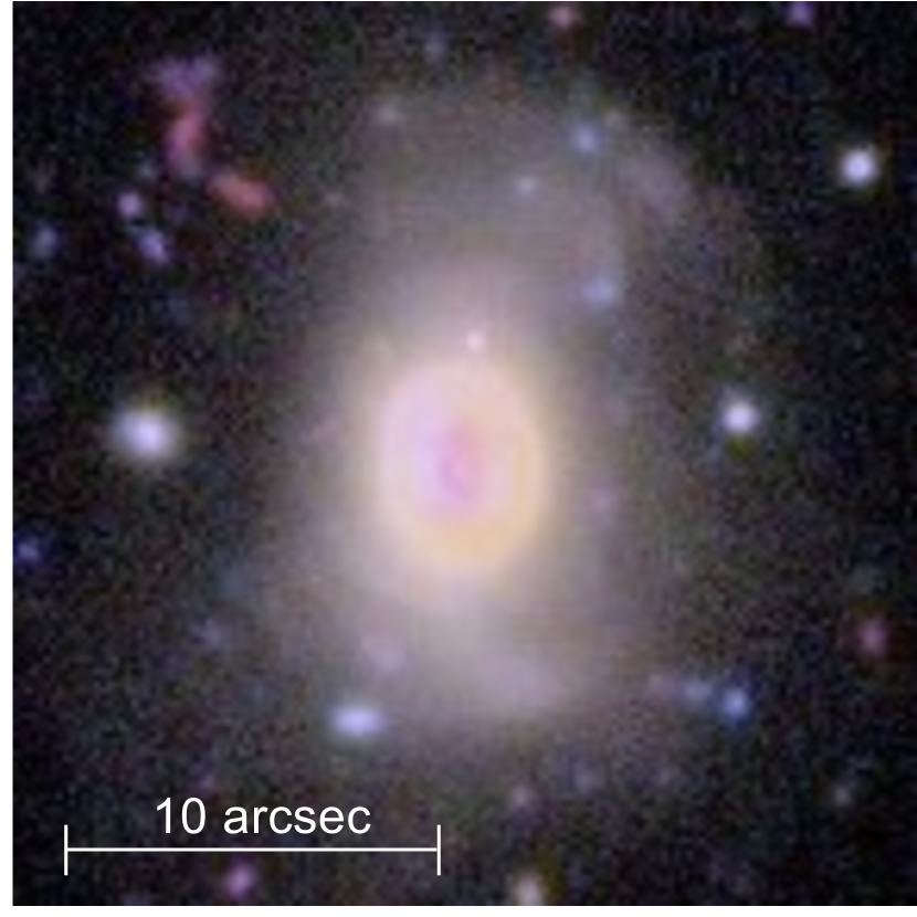
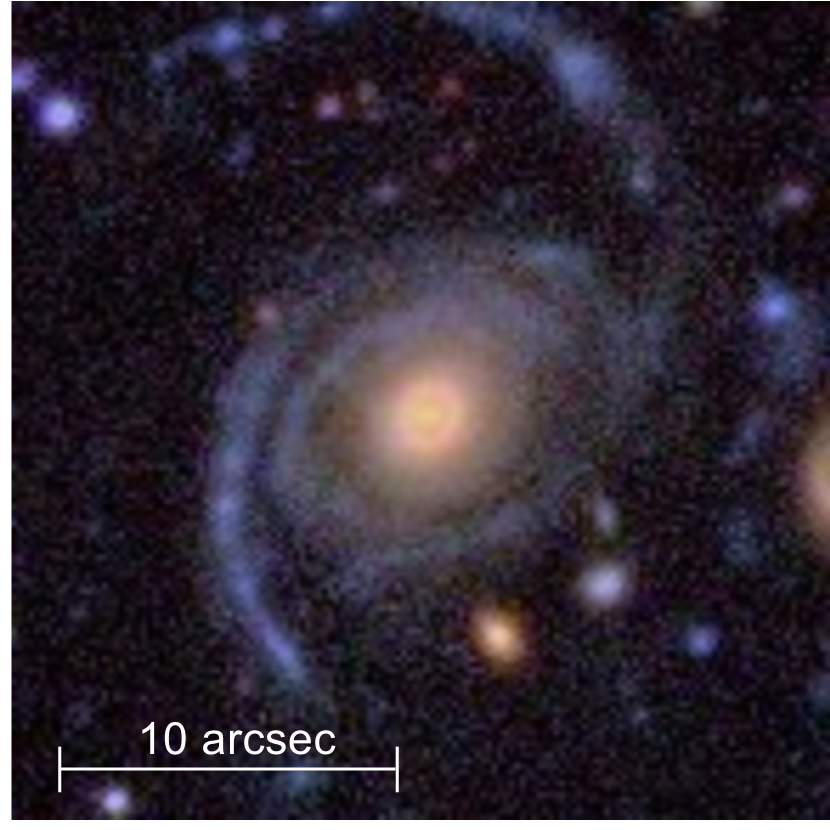
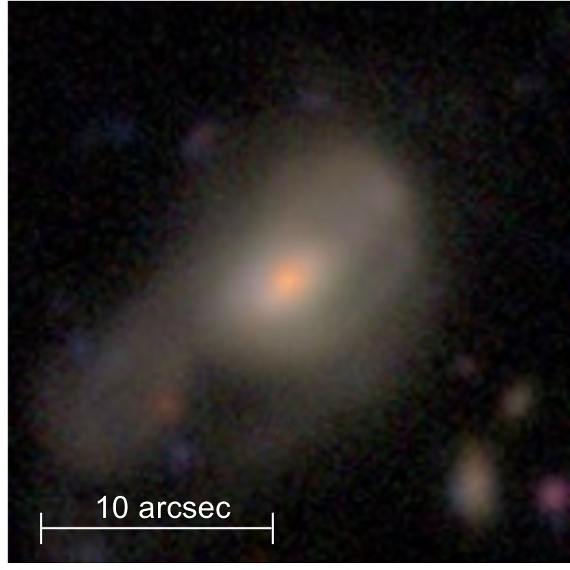
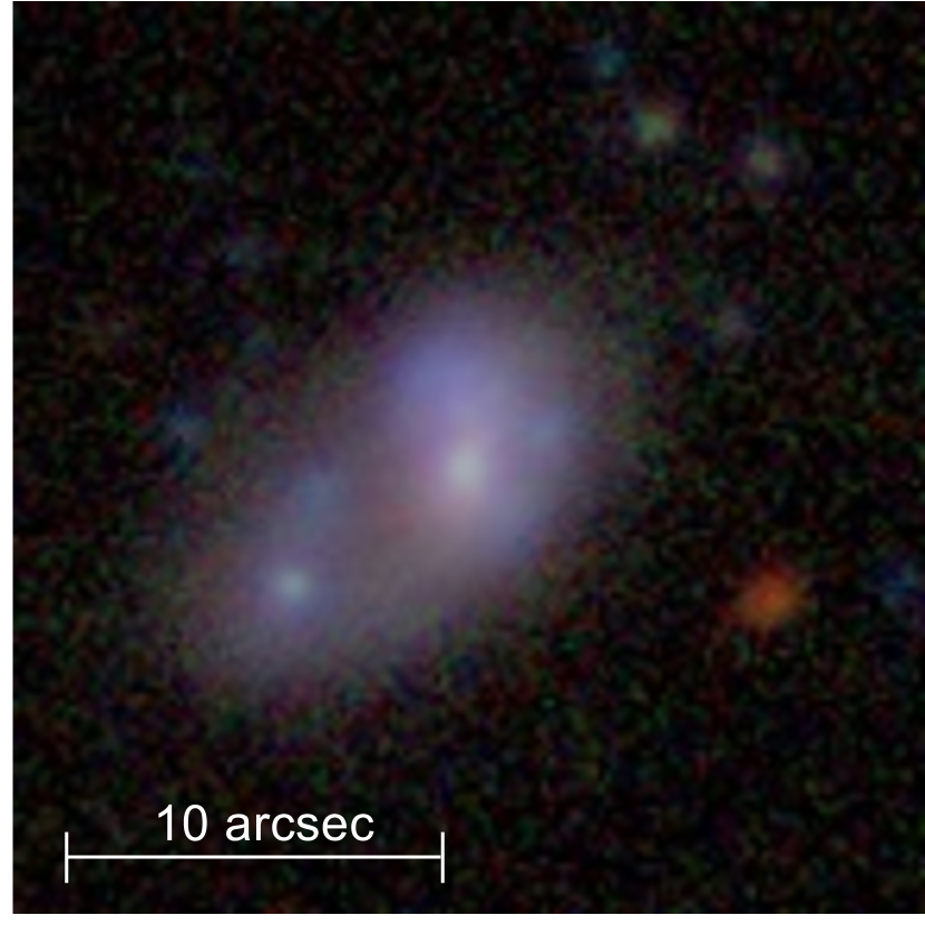
Figure 1: Example of galaxies with tidal features from HSC-SSP (gri-band cutout images). Top row from left to right: shells, stream. Bottom row from left to right: asymmetric halo, and double nucleus.

With the promising recent results of machine learning in galaxy classification tasks, we turn to machine learning to construct a model which can take galaxy images as input, convert them into representations - low-dimensional maps which preserve the important information in the image - and output a classification based on whether the galaxy exhibits tidal features. We are looking for a tool which can perform classification and be told what features to look for, so an unsupervised machine learning model is not ideal. We also want a tool which does not require large labelled datasets for training, due to there being few such datasets of galaxies with tidal features and these being time-demanding to construct in themselves, so a supervised model is not ideal either. Instead we use a recently developed machine learning method that is essentially a middle-point between supervised and unsupervised learning, known as self-supervised machine learning (SSL; He et al. 2019; Chen et al. 2020c; Chen et al. 2020b; Chen et al. 2020a; Chen & He 2020). Such models do not require labelled data for the training of the encoder, which learns to transform images into meaningful low-dimensional representations, but can perform classification when paired with a linear classifier and a small labelled dataset. Instead of labels, SSL models rely on augmentations (e.g. image rotation, noise addition, PSF blurring) being applied to the encoder training dataset, to learn under which conditions the output low-dimensional representations should be invariant. These types of models have been successfully used for a variety of astronomical applications (Huertas-Company et al., 2023) including classification of galaxy morphology (e.g. Walmsley et al. 2022; Wei et al. 2022; Ćiprijanović et al. 2023), clustering of galaxies according to age, metallicity, and velocity (e.g. Sarmiento et al. 2021), estimation of black hole properties (e.g. Shen et al. 2022), radio galaxy classification (e.g. Slijepcevic et al. 2022; Slijepcevic et al. 2023), and classification of solar magnetic field measurements (e.g. Lamdouar et al. 2022). Another benefit to self-supervised models, other than training on unlabelled data, is the computational cost, self-supervised models have been shown to need only 1% of the computational power needed by supervised models (Hayat et al., 2021). Self-supervised models are also much easier to adapt to perform new tasks, and apply to datasets from new data releases or different astronomical surveys (Ćiprijanović et al., 2023), making this kind of model perfect for our goal of applying a tool developed using HSC-SSP data to future LSST data and potentially other future large imaging surveys such as Euclid (Borlaff et al., 2022) and the Nancy Grace Roman Space Telescope (Spergel et al., 2015). Hayat et al. (2021) and Stein et al. (2022) show that once the encoder section of a self-supervised model has been trained one can conduct a simple similarity search to find objects of interest, or apply a linear classifier directly onto the encoder’s outputs to separate the data into a variety of classes.

In this paper, we demonstrate that SSL can be used to detect tidal features amidst a dataset of thousands of otherwise uninteresting galaxies using $\sim$50,000 $grizy$-band Hyper Suprime-Cam Subaru Strategic Program (HSC-SSP; Aihara et al. 2018) 128$\times$128 pixel galaxy images. We also show the advantage of using a self-supervised model, as opposed to a supervised model, for the detection of merging galaxies, particularly in the regime of fewer labels, using the dataset of $\sim$ 6000 Sloan Digital Sky Survey (SDSS; York et al. 2000) galaxies constructed by Pearson et al. (2019). In Section 2 we detail data and sample selection, as well as the model architecture, including the augmentations we apply to the data. Section 3 details our results including our model’s ability to detect tidal features in HSC-SSP data and a comparison of our model’s performance to a supervised model when used for the detection of merging galaxies in SDSS images. In Section 4 we compare our results with those in the literature and present our conclusions.

2 Methods

2.1 Data Sources and Sample Selection

For this work we use two separate datasets sourced from two different surveys. The first dataset is assembled from HSC-SSP galaxies and is used to show the potential of self-supervised machine learning models for the detection of tidal features. The second dataset consists of SDSS galaxies and is used to compare the performance of this self-supervised model with an earlier supervised model for the detection of merging galaxies.

2.1.1 HSC-SSP Dataset

The HSC-SSP dataset used for this work is sourced from the Ultradeep (UD) layer of the HSC-SSP Public Data Release 2 (PDR2; Aihara et al. 2019) for deep galaxy images. The HSC-SSP survey (Aihara et al., 2018) is a three-layered, grizy-band imaging survey carried out with the Hyper Suprime-Cam (HSC) on the 8.2m Subaru Telescope located in Hawaii. During the development of this project the HSC Public Data Release 3 (Aihara et al. 2022) became available. Although this is an updated version of the HSC-PDR2, we do not use this data due to the differences in the data treatment pipelines. HSC-PDR2 has been widely tested for low surface brightness studies (e.g. Huang et al. 2018, 2020; Li et al. 2022; Martínez-Lombilla et al. 2023) and fulfils the requirements for our study. The HSC-SSP survey comprises of three layers: Wide, Deep, and Ultradeep which are observed to varying surface brightness depths. We use the Ultradeep field, which spans an area of $3.5$ deg² and reaches $\mu_{r}\sim$ 29.82 mag arcsec^-2 (Martínez-Lombilla et al., 2023), a surface brightness depth faint enough to detect tidal features. We use HSC-SSP data not only for its depth, allowing us to detect tidal features, but also due to its similarity to LSST data. HSC-SSP data are reduced using the LSST pipeline (Bosch et al., 2018; Aihara et al., 2019) and since the two surveys produce similar data, it will be more straightforward to adapt our SSL model and train it on LSST data once it is released. The HSC-SSP PDR2 has a median $\it{i}$-band seeing of 0.6 arcsec and a spatial resolution of 0.168 arcsec per pixel.

We assemble our initial unlabelled dataset of $\sim$50,000 galaxies by parsing objects in the HSC-SSP PDR2 database using an SQL search and only selecting objects which satisfy a pre-defined criteria. We describe our criteria, their definitions, and our reasoning for choosing them in Table 1. We filter our sample of 50,000 galaxies to remove repeat objects in the dataset by removing objects whose declinations and right ascensions are too close together (within a 5 arcsec radius circle), leaving us with a dataset of $\sim$ 44,000 unlabelled objects. We access the HSC-SSP galaxy images using the Unagi Python tool (Huang et al., 2019) which, given a galaxy’s right ascension and declination, allows us to create multi-band ‘HSC cutout’ images of size 128 $\times$ 128 pixels ( 21 $\times$ 21 arcsecs), centred around each galaxy. Each cutout is downloaded in five ($g,~{}r,~{}i,~{}z,~{}y$) bands.

As mentioned in Section 1 self-supervised networks encode images into meaningful lower-dimensional representations but cannot inherently perform classification tasks. To perform the classification, we will be using a linear classifier which takes in the encoded representations as input and classifies galaxies based on the presence of tidal features. To train this linear classifier we require a small labelled dataset of galaxies with and without tidal features. We use the HSC-SSP PDR2 dataset assembled by Desmons et al. (2023) composed of 211 galaxies with tidal features and 641 galaxies without tidal features. These galaxies were selected from a volume-limited sample with spectroscopic redshift limits 0.04 $\leq$ z $\leq$ 0.2 and stellar mass limits 9.50 $\leq$ log₁₀($M_{\star}$/M_⊙) $\leq$ 11.00 and have i-band magnitudes in the range 12.8 < i < 21.6 mag. To increase the size of our tidal feature training sample we classified additional galaxies from our HSC-SSP PDR2 unlabelled dataset of $\sim$ 44,000 objects, according to the classification scheme outlined in Desmons et al. (2023). The classification was performed by the first author. We use an equal number of galaxies with and without tidal features for model training and testing to prevent the model from learning an accidental bias against the category with fewer images. Our final labelled sample contains 760 galaxies, 380 with tidal features, labelled 1, and 380 without, labelled 0. Usually a labelled dataset is split into 80%, 10%, and 10% for training, validation, and testing respectively. However our labelled dataset is small and we want to maximise the number of galaxies in our testing dataset such that the model can be evaluated accurately. Hence we split our labelled dataset set into training, validation, and testing datasets composed of 600 (79%), 60 (8%), and 100 (13%) galaxies respectively.

Table 1: Criteria used in our SQL search to select our training sample. An ‘x’ indicates the cut was applied to each band $(g,r,i,z,y)$.

Criteria	Definition and Reasoning
15 < i_cmodel_mag < 20	$i-$band flux (mag) from the final cmodel fit. We set a faint magnitude limit of 20 mag to ensure that objects are bright enough for tidal features to be visible.
x_inputcount_value $\geq$ 3	The number of exposures available in a given band. We only select images which have at least 3 exposures in each band $(g,r,i,z,y)$ to ensure galaxies have full depth and colour information.
NOT x_pixelflags_bright_objectcenter NOT x_pixelflags_bright_object	Flags objects which are affected by bright sources. We set this criterion to avoid selecting objects affected by bright stars.
NOT x_pixelflags_edge	Flags objects which intersect the edge of the exposure region. Ensures that objects are fully visible and not cut off by the edge of a region.
NOT x_pixelflags_saturatedcenter	Flags objects which have saturated central pixels. We set this to avoid selecting objects with saturated pixels.
NOT x_cmodel_flag	Flags objects which have general cmodel fit failures. Ensures we only select objects with good photometry.
i_extendendness_value > 0.5	Provides information about the extendedness of an object, values $<$ 0.5 indicate stars. We set this $>$ 0.5 to ensure we only select galaxies and not stars.

2.1.2 SDSS Dataset

Our second dataset, consisting of SDSS data release 7 (Abazajian et al., 2009) galaxies, was assembled by Pearson et al. (2019) for the purpose of training a supervised network to classify merging and non-merging galaxies. This dataset contains $\sim$ 10,000 non-merging galaxies and $\sim$ 3000 merging galaxies which were selected from the Darg et al. (2010a, b) catalogue, assembled from Galaxy Zoo (Lintott et al., 2008) classifications. All galaxies in this dataset have spectroscopic redshift limits 0.005 $\leq$ z $\leq$ 0.1 and are in the stellar mass range 9.5 $\leq$ log₁₀($M_{\star}$/M_⊙) $\leq$ 12.0. Additionally, they were required to have SDSS spectra, which were only taken for objects with apparent magnitude $r~{}<$ 17.7 mag. Due to this magnitude limit being significantly brighter than the HSC-SSP dataset described above, only the brightest tidal features would be visible in these images. This means that the merging galaxies in this sample were selected not based on the presence of tidal features, but rather based on whether galaxies showed obvious signs of mergers with at least two clearly interacting galaxies or significantly morphologically disturbed systems. To prevent the model learning an accidental bias against the category with fewer images we reduce the size of our non-merging dataset by randomly selecting only 3000 non-merging galaxies from the set of 10,000. The SDSS dataset used to train and test our model now consists of 3000 merging galaxies, labelled 1, and 3000 non-merging galaxies, labelled 0. This gives us a sample of 6000 SDSS objects of which we obtain 256 $\times$ 256 pixel images, downloaded in three ($g,~{}r,~{}i$) bands. For more detail about the construction and classification of the SDSS dataset we refer the reader to Pearson et al. (2019). When a labelled dataset is required for training (i.e. for the supervised model or the linear classifier) we split this dataset into 4800 (80%), 600 (10%), and 600 (10%) galaxies to use for training, validation, and testing respectively. For the portion of the training of our self-supervised model which requires an unlabelled dataset, we increase the size of our SDSS dataset from 6000 galaxies to 50,000 galaxies. This is done by making the dataset repeat, selecting 50,000 samples of the 6000 galaxies, and randomly rotating each image 0, 90, 180, or 270 degrees to create ‘new’ images.

The analysis presented in Section 3 is focused on comparing the performance of supervised and self-supervised models when a varying number of labels are used for training. When using fewer labels to train a model, we do not reduce the number of images shown to the model during training, but rather the number of unique images. For example, if the model trained on 80% of the full SDSS training set is shown 4800 unique images, the model trained on 2% of the labelled data is still shown 4800 images but only 120 of these images are unique. This ensures that the change in model performance is indeed due to the number of unique labelled examples, and not due to the model being shown fewer images.

2.2 Image Pre-processing and Augmentations

Before the images are augmented and fed through the model we apply a pre-processing function to normalise the images. For the HSC-SSP images this is done by taking a subsample of 1000 galaxies from our unlabelled training sample and calculating the standard deviation $\sigma_{\text{pixel count}}$ for each band $(g,r,i,z,y)$ of this subsample using the median absolute deviation. The entire sample is then normalised by dividing each image band by the corresponding $3\sigma$ and then taking the hyperbolic sine of this. In this step we also define an ‘unnormalising’ function which does the inverse of the normalising function, allowing us to retrieve the original unormalised images if needed. The SDSS images we obtained from Pearson et al. (2019) were already in PNG format with pixel values between 0 and 255. To normalise these we simply divide each image band by 255.

Self-supervised networks work by encoding images into lower-dimensional representations and using augmented versions of the training images to learn under which transformations the encoded representations should be invariant. More specifically, these networks use contrastive loss (Hadsell et al., 2006) which is minimised for different augmentations of the same image, and maximised when the images are different. These augmentations are defined and applied before the images get processed by the network and are chosen based on the task at hand. In this project we are constructing a network to classify whether a galaxy possesses tidal features. This classification should be independent of the level of noise, or the orientation or position of the galaxy in the image. To achieve this we use the following augmentations:

• Orientation: We randomly flip the image across each axis (x and y) with 50% probability.

• Gaussian Noise: We sample a scalar from $\mathcal{U}$(1,3) and multiply it with the median absolute deviation of each channel (calculated over 1000 training examples) to get a per-channel noise $\sigma_{c}$. We then introduce Gaussian noise sampled from $\sigma_{c}~{}\times~{}\mathcal{N}$(0,1) for each channel.

• Jitter and Crop: For HSC-SSP images we crop the 128 $\times$ 128 pixel image to the central 109 $\times$ 109 pixels before randomly cropping the image to 96 $\times$ 96 pixels. Random cropping means the image centre is translated, or ‘jittered’, along each respective axis by $i$, $j$ pixels where $i$, $j~{}\sim~{}\mathcal{U}$(-13,13) before cropping to the central 96 $\times$ 96 pixels. For SDSS images we crop the 256 $\times$ 256 pixel image to the central 72 $\times$ 72 pixels before randomly cropping the image to 64 $\times$ 64 pixels. We use 64 $\times$ 64 pixel images when training with SDSS data as these are the image dimensions used by Pearson et al. (2019) for their model. We use a smaller maximum centre translation ($i$, $j~{}\sim~{}\mathcal{U}$(-8,8)) for SDSS images due to their smaller size.

2.3 Model Architecture

The model we utilise to perform classification of tidal feature candidates consists of two components; a self-supervised model used for pre-training, and a linear classifier used for classification. The self-supervised model receives galaxy images as input and encodes these into meaningful lower-dimensional representations. The linear classifier is a simple supervised model which takes in galaxy images, encodes them into representations using the trained self-supervised model, and outputs a binary classification. All models described below are built using the TensorFlow framework (Abadi et al., 2016).

2.3.1 The Self-Supervised Architecture

For our task of classifying tidal feature candidates we use a type of self-supervised learning known as Nearest Neighbour Contrastive Learning of visual Representations (NNCLR; Dwibedi et al. 2021). We closely follow Dwibedi et al. (2021) in designing the training process for our model. A general schematic of the NNCLR framework is shown in Figure 2 and we refer the reader to Dwibedi et al. (2021) for a more detailed explanation of the approach.

Self-supervised models rely on augmentations to create different views of the same images. Given a sample of images x, a pair of images ($\mathrm{\mathbf{x_{i}}}$, $\mathrm{\mathbf{x_{j}}}$) is defined as positive when $\mathrm{\mathbf{x_{j}}}$ is an augmented version of image $\mathrm{\mathbf{x_{i}}}$, a positive pair can be expressed as ($\mathrm{\mathbf{x_{i}}}$, $\mathrm{\mathbf{x_{i}^{+}}}$). If $\mathrm{\mathbf{x_{j}}}$ is not an augmented version of image $\mathrm{\mathbf{x_{i}}}$ the pair is negative and is expressed as ($\mathrm{\mathbf{x_{i}}}$, $\mathrm{\mathbf{x^{-}}}$). For each of the images in x, an encoder networks creates a 128 dimensional representation z = encoder(x). This encoder is trained to make the representations similar for positive pairs, and dissimilar for negative pairs, by using a contrastive loss function:

$$L_{i}=-\log\left(\frac{\mathrm{exp(sim(\mathbf{z_{i}},\mathbf{z_{i}^{+}}))}}{\mathrm{exp(sim(\mathbf{z_{i}},\mathbf{z_{i}^{+}}))}+\sum\mathrm{\mathbf{{}_{z^{-}}}exp(sim(\mathbf{z_{i}},\mathbf{z^{-}}))}}\right)$$ (1)

where sim(a, b) = a $\cdot$ b /  ($\tau||\rm{\textbf{a}}||~{}||\rm{\textbf{b}}||$) is the cosine similarity between vectors a and b, normalised by the tunable "softmax temperature" $\tau$. This contrastive loss, or InfoNCE loss (Oord et al., 2018), is minimised when the similarity is high for positive pairs and low for negative pairs. Using this contrastive loss, self-supervised networks learn to make the representations similar for positive pairs, and dissimilar for negative pairs, and hence are able to cluster similar (or positive) samples together and push apart dissimilar (or negative) samples. These contrastive learning methods (e.g. SimCLR; Chen et al. 2020a) rely only on differently augmented views of the same image to create positive pairs. As a consequence, objects which exhibit large variations but belong to the same class (e.g. galaxies with different types of tidal features) might not be linked using this type of method. NNCLR methods aim to resolve this issue by creating a more diverse set of positive pairs. Instead of defining positive pairs as ($\mathrm{\mathbf{x_{i}}}$, $\mathrm{\mathbf{x_{i}^{+}}}$) where $\mathrm{\mathbf{x_{i}^{+}}}$ is an augmented version of image $\mathrm{\mathbf{x_{i}}}$, NNCLR uses a queue of examples $\mathcal{Q}$, and defines $\mathrm{\mathbf{x_{i}^{+}}}$ as the nearest-neighbour of $\mathrm{\mathbf{x_{i}}}$ in the queue. The loss function for NNCLR models varies slightly from the InfoNCE loss and is defined as:

$$L_{i}^{\rm{NNCLR}}= -\log\left(\frac{\mathrm{exp(NN(\mathbf{z_{i}},\mathcal{Q})~{}\cdot~{}\mathbf{z_{i}^{+}}~{}/~{}\tau)}}{\sum\mathrm{\mathbf{{}_{k}}exp(NN(\mathbf{z_{i}},\mathcal{Q})~{}\cdot~{}\mathbf{z_{k}^{+}}~{}/~{}\tau)}}\right)$$

$$-\log\left(\frac{\mathrm{exp(NN(\mathbf{z_{i}},\mathcal{Q})~{}\cdot~{}\mathbf{z_{i}^{+}}~{}/~{}\tau)}}{\sum\mathrm{\mathbf{{}_{k}}exp(NN(\mathbf{z_{k}},\mathcal{Q})~{}\cdot~{}\mathbf{z_{i}^{+}}~{}/~{}\tau)}}\right)$$

where NN($\mathrm{\mathbf{x_{q}}}$, $\mathcal{Q}$) is the nearest neighbour operator defined as:

$$\mathrm{NN(\mathbf{z},\mathcal{Q})}=\mathop{\arg\min}\limits_{i\in\mathcal{Q}}~{}||\mathrm{\mathbf{z}}-i||_{2}$$ (2)

where $||\mathrm{\mathbf{x}}||_{2}$ represents $\mathrm{\mathbf{x}}$ $l_{2}$-normalised along the first axis, defined as:

$$||\mathrm{\mathbf{x}}||_{2}=\sqrt{\sum_{k=1}^{n}|x_{k}|^{2}}$$ (3)

The self-supervised model was trained using a temperature of 0.1 and a queue size of 10,000. Following Hayat et al. (2021) and Stein et al. (2021a), we use ResNet-50 (He et al., 2016) as our encoder followed by an global pooling layer. The architecture of the projection head is two fully connected layers of size 128, which use L2 kernel regularisation with a penalty of 0.0005. Each fully connected layer is followed by a batch-normalisation layer, and the first batch-normalisation layer is followed by ReLU activation. The model was compiled using the Adam optimiser (Kingma & Ba, 2015) and trained for 25 epochs on our unlabelled dataset of $\sim$ 44,000 HSC-SSP PDR2 galaxies or our dataset of 50,000 SDSS galaxies. Training was completed within $\sim$ 30 minutes using a single GPU.

Figure 2: Illustration of the self-supervised model architecture. The model takes in a batch of images as input and creates two different views of the batch using random augmentations. Each view is encoded and the nearest neighbour of view 1 is located from the queue of example images. The loss between view 2 and the nearest neighbour of view 1 is calculated using a contrastive loss function which is minimised for similar pairs of images and maximised otherwise.

2.3.2 The Linear Classifier Architecture

The second part of the model is a simple linear classifier which takes galaxy images as input and converts them to representations using the pre-trained self-supervised encoder. These encoded representations are passed through a fully connected layer with a sigmoid activation, which outputs a single number between 0 and 1. This fine-tuned model was compiled using the Adam optimiser (Kingma & Ba, 2015) and a binary cross entropy loss. It was trained for 50 epochs using the labelled training set of 600 HSC-SSP galaxies or 4800 SDSS galaxies. Training was completed within $\sim$ 1 minute using a single GPU.

2.3.3 The Supervised Architecture

To draw conclusions about the suitability of self-supervised models for the detection and classification of tidal features, we compare our results with those of a fully supervised model. We do not construct this model from scratch, but instead use the model designed by Pearson et al. (2019) to classify merging galaxies. This model consists of four convolutional layers, each followed by a Rectified Linear unit (ReLU) activation layer and a dropout layer with a dropout rate of 20%. The first, second, and fourth convolutional layers also have max-pooling layers following the dropout layers. The model then has two dense layers, each followed by a ReLU activation layer and dropout layer. The final layer is a dense layer which has two neurons and softmax activation. We do not detail the dimensions of the network layers here but instead focus on the changes made to adapt the network to our data. For further detail on the architecture of this network we refer the reader to Pearson et al. (2019). The output layer was changed from two neurons with softmax activation, to a single neuron with sigmoid activation. The network was compiled using the Adam optimiser (Kingma & Ba, 2015) with the default learning rate and loss of the network was determined using binary cross entropy. When training the network on our HSC-SSP dataset we additionally changed the input image dimension from 64 $\times$ 64 pixels with three colour channels to 96 $\times$ 96 pixels with five colour channels. We do this because tidal features in deeper images can often be seen to extend around the galaxy and using 64 $\times$ 64 pixel images can cause them to be cut-off. We train the supervised network from scratch using the labelled training set of 600 HSC-SSP galaxies or 4800 SDSS galaxies.

2.4 Model Evaluation

There are a number of metrics used in the literature to evaluate the performance of machine learning models, depending on the task at hand. The purpose of our model is to partially automate the creation of large datasets of galaxies with tidal features by reducing the amount of data which has to be visually classified. If the top $N$ predictions will be visually classified, we want to maximise the number of true positives, or galaxies with tidal features, in the top $N$ predictions while minimising the number of false positives, or galaxies without tidal features. As such, in terms of model performance, we are primarily concerned with the true positive rate (also known as recall or completeness) and false positive rate (also known as fall-out or contamination). The true positive rate (TPR) ranges from 0 to 1 and is defined as:

$$TPR=\frac{TP}{TP~{}+~{}FN}$$ (4)

where $TP$ is the number of true positives (i.e. the number of galaxies with tidal features correctly classified by the model) and $FN$ is the number of false negatives (i.e. the number of galaxies with tidal features incorrectly classified by the model). The false positive rate (FPR) also ranges from 0 to 1 and is defined as:

$$FPR=\frac{FP}{FP~{}+~{}TN}$$ (5)

where $FP$ is the number of false positives (i.e. the number of galaxies without tidal features incorrectly classified by the model) and $TN$ is the number of true negatives (i.e. the number of galaxies without tidal features correctly classified by the model).

In addition to using the TPR for a given FPR to evaluate our model, we also use the area under the receiver operating characteristic (ROC) curve to evaluate performance. The ROC curve is a plot of the TPR against the FPR for a range of threshold values, which is the threshold between outputs being labelled positive or negative. For our model where galaxies with tidal features are labelled 1 and galaxies without are labelled 0, the threshold can take any value between 0 and 1 and determines whether outputs are classified as galaxies with or without tidal features. The area under the ROC curve (AUC) of a perfect model with TPR$~{}=~{}1$ and FPR$~{}=~{}0$ is unity, while a good model will have an AUC close to unity. A truly random model will have a ROC AUC of 0.5.

3 Results

In this section we first compare the performance of our self-supervised model with a supervised model, before exploring how our self-supervised model organises the galaxy images in representation space.

3.1 Self-Supervised vs. Supervised Performance

Figure 3 illustrates the ROC AUC for a supervised and self-supervised network as a function of percentage of labels used in training for our SDSS dataset. As shown, when the amount of training data is within the range of 80% (4800 labels) to 10% (600 labels) the models show very similar performances. However, in the regime of fewer labels, particularly when training with 5% (300) or 2% (120) unique labelled examples, both models show decreased performance but this decrease is significantly greater for the supervised model. When 2% (120) of labelled training data is used, the self-supervised model AUC only decreases to 0.85 while the supervised AUC drops to 0.77. This figure does not show that self-supervised models can be used in the detection of tidal features, because the criterion for galaxies being classed as merging in the SDSS dataset is mainly based on whether two clearly interacting galaxies could be seen in the images.

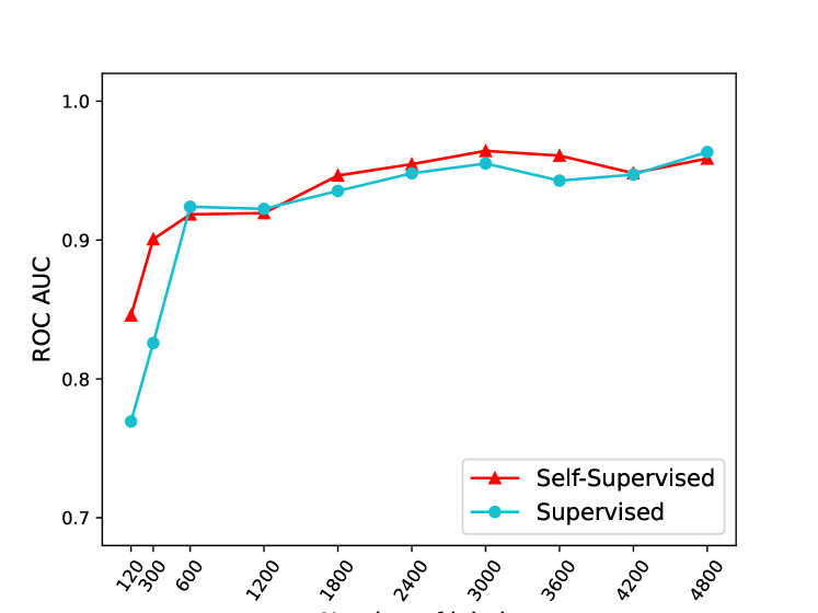
Figure 3: ROC AUC as a function of the percentage of SDSS labels used for training for a supervised (blue) and self-supervised (red) model. 80% of labels is equal to 4800 labels. Both models show similar performance in the high number of labels regime. For fewer training labels, the self-supervised model outperforms the supervised model.

To show that self-supervised models can be used to detect galaxies with tidal features we rely on our HSC-SSP dataset, which reaches surface brightness depths sufficient to clearly identify tidal features. Figure 4 illustrates the testing set ROC AUC for a supervised and self-supervised network as a function of the number of labels used in training for our HSC-SSP dataset. Each point represents the ROC AUC averaged over ten runs using the same training, validation, and testing sets for each run. We average the ROC AUC over the 10 runs and remove outliers further than $3\sigma$ from the mean. It is important to note that in this figure, the number of labels for our rightmost data point, where 600 labels are used for training, is equivalent to the 10% of labels data point for the SDSS results in Figure 3. Our SSL model maintains high performance across all amounts of labels used for training, having ROC AUC $=$ 0.911 $\pm$ 0.002 when training on the maximum number of labels and only dropping to ROC AUC $=$ 0.89 $\pm$ 0.01 when using only 50 labels for training. This is in contrast to the supervised model, which also maintains its performance regardless of label number, but only reaches ROC AUC $=$ 0.867 $\pm$ 0.004 when training on the maximum number and ROC AUC $=$ 0.83 $\pm$ 0.01 when using only 50 labels for training.

This figure not only shows that a SSL model can be used for the detection of tidal features with good performance, but also that it performs consistently better than the supervised network regardless of the number of training labels.

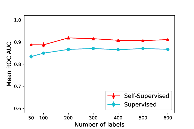
Figure 4: Average ROC AUC as a function of the number of HSC-SSP labels used for training for a supervised (blue) and self-supervised (red) model. Each point is an average of ten runs. Both models are able to classify galaxies with tidal features. The self-supervised model performs consistently better, but both models remain consistent for all number of labels.

It seems unlikely that a purely supervised network would maintain such good performance with only 50 unique labelled training examples, however, upon inspection we found no problems with our dataset assembly or model training. Instead of only evaluating the model based on its performance with regards to the testing set, we also plot the results of the models based on the validation loss. We do this by choosing the ‘best’ model from the ten runs for each number of labels, defined as the model which reaches the lowest validation loss at the end of training. Typically, a lower validation loss translates to a better model performance on the testing set. However, our validation and testing sets are very small, 60 and 100 galaxies respectively, making it hard to evaluate our models accurately using just one method.

In Figure 5 we show the testing set ROC AUC for a supervised and self-supervised network as a function of the number of labels used for training. This time, instead of each point being an average of ten runs, we show the result of the model which reached the lowest final validation loss for the given number of labels used for training. This figure shows that both models maintain similar ROC AUC when using more training labels, however, when using less than 300 labels for training, the supervised model begins to decrease in performance. When using as few as 50 labelled examples for training, the self-supervised model’s ROC AUC remains stable around 0.9, whereas the supervised model’s ROC AUC drops to 0.7. Although this may seem to contradict the results of Figure 4, the two figures compare different methods of assessing the model. Figure 4 is based only on the performance of the model on the testing set, whereas Figure 5 takes into account the training process using the validation loss. The self-supervised network shows consistency in the ROC AUC regardless of which method is chosen to evaluate the model, while the supervised network appears to be more sensitive to the choice of method.

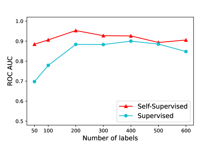
Figure 5: ROC AUC as a function of the number of HSC-SSP labels used for training for a supervised (blue) and self-supervised (red) model. Each point shows the ROC AUC for the model which reached the lowest final validation loss for the given number of training labels. Both models show similar performance in the high number of labels regime. For fewer training labels, the self-supervised model outperforms the supervised model.

Figure 4 showed that our SSL model maintained its ROC AUC and performed consistently better than the supervised network regardless of the number of training labels. This result is also reflected in Figure 6 which shows the testing set TPR for FPR $=$ 0.2 for our supervised and self-supervised networks as a function of the number of labels used in training. Similar to Figure 4, each point represents the TPR averaged over 10 runs, removing outliers further than $3\sigma$ from the mean. Figure 6 not only shows that the TPR for a given FPR is consistently higher for our self-supervised model than our supervised model but also that the self-supervised model mantains a high TPR regardless of the number of training labels, only dropping from TPR $=$ 0.94 $\pm$ 0.01 at 600 training labels to TPR $=$ 0.90 $\pm$ 0.01 with a mere 50 training labels.

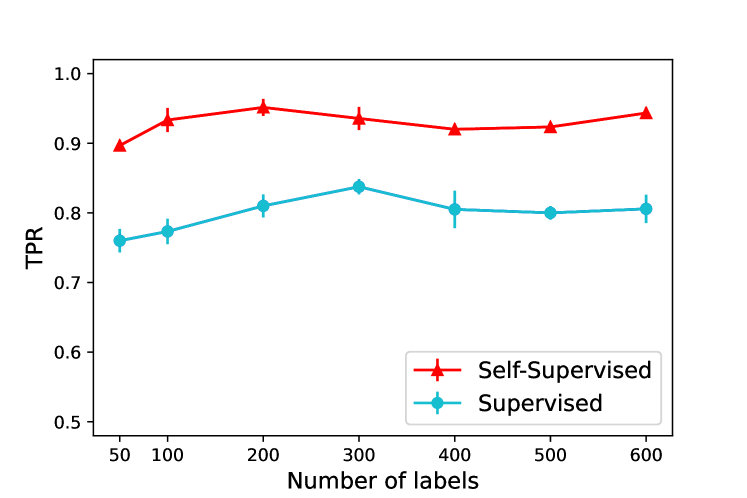
Figure 6: Average TPR when FPR $=$ 0.2 as a function of the number of HSC-SSP labels used for training for a supervised (blue) and self-supervised (red) model. Each point is an average of 10 runs. Both models show a slight decrease in TPR with decreasing training label number. The self-supervised model has a consistently higher TPR.

3.2 Detection of Tidal Features

One advantage of self-supervised models over supervised models is the ability to use just one labelled example to find examples of similar galaxies from the full dataset. By using just one image from our labelled tidal feature dataset as a query image, and the encoded 128-dimensional representations from the self-supervised encoder, we can perform a similarity search that assigns high similarity scores to images which have similar representations to the query image. This is done using a similarity function which takes in the encoded representations of two images, $l_{2}$-normalises them along the first axis, and returns the reduced sum of the product of these normalised representations. This is demonstrated in Figure 7 where we select two galaxies with tidal features from our training sample and perform a similarity search with the 44,000 unlabelled HSC-SSP galaxies. In Figure 7 the query image is shown on the right alongside the 24 galaxies which received the highest similarity scores. This figure shows the power of self-supervised learning, where using only a single labelled example, we can find a multitude of other tidal feature candidates.

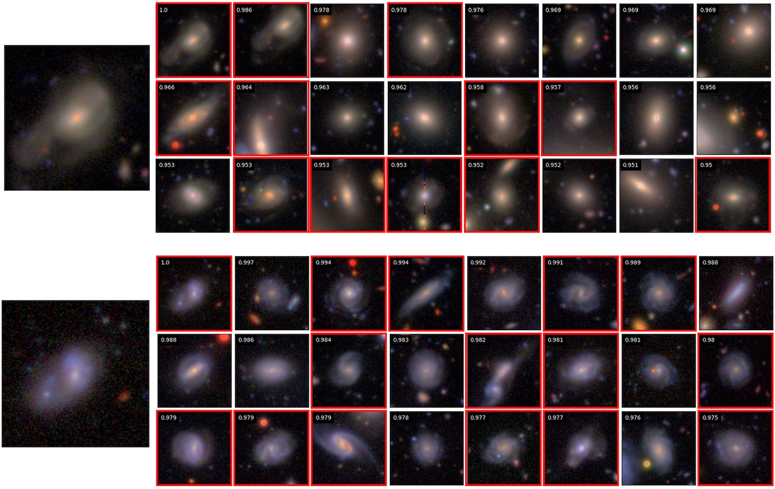
Figure 7: Results from a similarity search using two random galaxies with tidal features as query images. The two query galaxies are displayed on the left, alongside the top 24 galaxies with the highest similarity scores for each similarity search. The similarity score is displayed in the top left corner for each image. The red outlines indicate galaxies which would be visually classified as hosting tidal features, regardless of whether this galaxy is the central object in the image.

Another way to visualise how the model organises the galaxy images in representation space, without having to select a query image, is by using Uniform Manifold Approximation and Projection (UMAP; McInnes et al. 2018). UMAP can be trained directly on image data to produce meaningful clusters however here we use it merely for visualisation purposes. UMAP takes in our encoded 128-dimensional representations as input and reduces them to an easier to visualise 2 dimensional projection. Figure 8 illustrates this 2D projection, created by binning the space into $100~{}\times~{}100$ cells and randomly selecting a sample from that cell to plot in the corresponding cell location. To obtain an idea of what attributes galaxy groupings are based on, we hand-select three areas and show zoomed-in versions of these areas around the edges of the figure. From this, it is clear that galaxies are grouped both according to their colour, and their size in the cutout. The fact that we can achieve a high performance of tidal feature classification (shown in Section 3.1) by simply using a linear classifier on the representations means that the representations created by the self-supervised encoder are meaningful. We also determine whether the scores given to galaxies by the linear classifier are related to the galaxies’ positions in the UMAP projection. This is done by colouring the UMAP plot according the scores given to each galaxy by the linear classifier, shown in the right panel of Figure 8. We find that the majority of galaxies which were assigned a high classifier score, indicating a high likelihood of tidal features, are located on the left side of the UMAP projection plot. This reinforces the idea that the encoded representations contain meaningful information about tidal features, but also brings to light a potential bias of our model. The left side of the UMAP projection plot contains the galaxies which cover more of the cutout, indicating a potential bias towards classifying bright galaxies that appear large in the cutouts as having tidal features. This bias is likely an effect of a bias potentially introduced by the training set, as tidal features are more likely to be visible and obvious for brighter and larger-appearing galaxies and hence these galaxies are more likely to be classified as having tidal features.

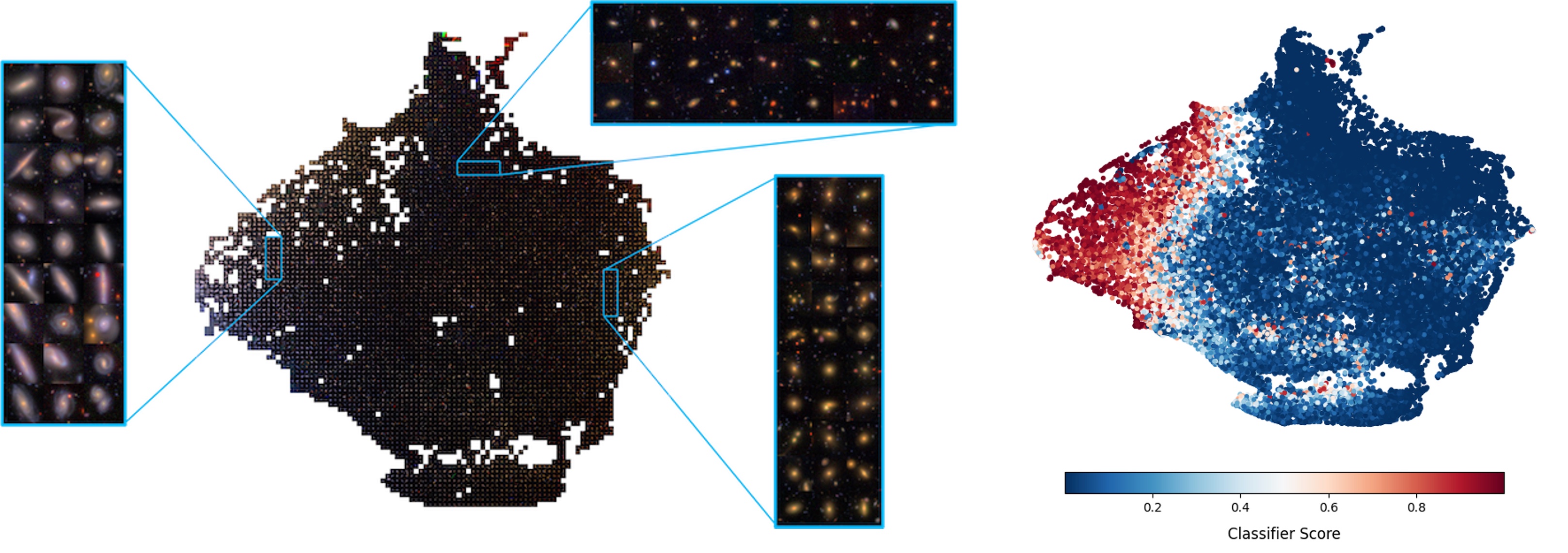
Figure 8: Left: 2D UMAP projection of the self-supervised representations. Made by binning the space into $100~{}\times~{}100$ cells and randomly selecting a sample from that cell to plot in the corresponding cell location. Right: The same 2D UMAP projection without binning, coloured according to the scores assigned to each galaxy by the linear classifier.

4 Discussion and Conclusions

In this work, we have shown that SSL models composed of a self-supervised encoder and linear classifier can not only be used to detect galaxies with tidal features, but can do so reaching both high completeness (TPR $=$ 0. 94 $\pm$ 0.1) for low contamination (FPR $=$ 0.20) and high area under the ROC curve (ROC AUC $=$ 0.91 $\pm$ 0.002). This means that such models can be used to isolate the majority of galaxies with tidal features from a large sample of galaxies, thus drastically reducing the amount of visual classification needed to assemble a large sample of tidal features. One major advantage of this model over other automated classification methods, is that this level of performance can be reached using only 600 labelled training examples, and only drops mildly when using a mere 50 labels for training maintaining ROC AUC $=$ 0.89 $\pm$ 0.01 and TPR $=$ 0.90 $\pm$ 0.1 for FPR $=$ 0.2. SSL models are also inexpensive to train, with the encoder needing only $\sim$ 30 minutes to train for 25 epochs on a single GPU. The linear classifier, applied to the encoded representations, only required $\sim$ 1 minute to train for 50 epochs on a single GPU. This makes SSL models easy to re-train on data from different surveys with minimal visual classification needed.

Previous works which used SSL models for classification of astronomical objects highlighted a number of advantages of these models compared to fully supervised models. Stein et al. (2021b) highlighted the usefulness of being able to use the encoded representations straight from the self-supervised encoder to perform similarity searches based on a single example image in the context of finding strong gravitational lens candidates. Hayat et al. (2021) emphasised the superior performance of their SSL model compared to a supervised model for both galaxy morphology classification, and spectroscopic redshift estimation, particularly when decreasing the number of labels available for training. In this work we find similar advantages of a SSL model compared to a supervised model. When using the models to detect merging galaxies from an SDSS dataset, both models show similar performance when using a larger number of training labels, however, in the regime of fewer training labels, the supervised model performance decreases more drastically than the SSL model. When using the models for the detection of tidal features we find that the SSL model consistently outperforms the supervised model, regardless of the number of labels used for training. Following Stein et al. (2021b), we emphasise the usefulness of being able to perform a similarity search using just the self-supervised encoder and one example of a galaxy with tidal features to find other galaxies with tidal features from a dataset of tens of thousands of galaxies.

The level of comparison that can be carried out with respect to the results obtained here and other works is limited due to the scarcity of similar works. There are only two studies focusing on the detection of tidal features using machine learning. The first is the work of Walmsley et al. (2019) who used a supervised network to identify galaxies with tidal features from the Wide layer of the Canada-France-Hawaii Telescope Legacy Survey (Gwyn, 2012). They used a sample of 305 galaxies with tidal features and 1316 galaxies without tidal features, assembled by Atkinson et al. (2013), to train a CNN, using augmentations such as image flipping, rotation, and translation to expand their dataset. Walmsley et al. (2019) found that their method outperformed other automated methods of tidal feature detection, reaching 76% completeness (or TPR) and 22% contamination (or FPR). Our SSL model, trained on 600 (300 tidal, and 300 non-tidal) galaxies performs considerably better, reaching a completeness of 96% for the same contamination percentage. Domínguez Sánchez et al. (2023) used this same CNN, designed by Walmsley et al. (2019), and the dataset presented in Martin et al. (2022) to also identify galaxies exhibiting tidal features. This dataset consists of $\sim$ 6000 synthetic mock HSC-SSP images, including $\sim$ 1800 galaxies with tidal features, from the NewHorizon cosmological hydrodynamical simulation at five different surface brightness limits, ranging from $\mu_{r}=$ 28 mag $\rm{arcsec}^{-2}$ to $\mu_{r}=$ 35 mag $\rm{arcsec}^{-2}$. They found that the model was able to successfully identify tidal features, reaching ROC AUC > 0.9 and a completeness of $\sim$ 90% for 22% contamination. They also separated the performance of the model according to the image surface brightness limits and found that at surface brightness limits close to HSC-SSP UD limits ($\mu_{r}\sim$ 28 mag $\rm{arcsec}^{-2}$) the model reached ROC AUC = 0.88 and completeness of $\sim$ 83% for 22% contamination. The ROC AUC reached by our model (0.911 $\pm$ 0.002) is comparable to that found in Domínguez Sánchez et al. (2023), however, we reach a significantly higher completeness of 96% for the same level of contamination. Domínguez Sánchez et al. (2023) also attempted to apply their trained model to real HSC-SSP images, however the model performance decreased significantly, only reaching ROC AUC = 0.64. They noted that this drop in performance could be attributed to the difference in angular resolution between the simulated and real images, or the lack of real background in the simulated images which were used to train their model.

In a similar work, Bickley et al. (2021) used a CNN to identify recently merged galaxies in a sample of galaxies from the cosmological magnetohydrodynamical simulation IllustrisTNG (Nelson et al., 2018). Their dataset was constructed by combining IllustrisTNG images with Canada France Imaging Survey (CFIS; Ibata et al. 2017) image data and metadata to create synthetic CFIS images and the sample consisted of $\sim$75,000 galaxies, including $\sim$37,000 recently merged galaxies. Their CNN achieved good performance, reaching a higher ROC AUC of 0.95 than our SSL model, and a similar completeness of $\sim$95% for 22% contamination, although their model required much larger labelled training set compared to our dataset of 600 galaxies. Bickley et al. (2021) also compared the performance of their CNN to that of visual identification performed by 9 classifiers on a subsample of 200 galaxies. They found that although the CNN recovered a higher fraction of the recently merged galaxies, the visual classifiers were capable of achieving higher purity in their classification. Bickley et al. (2021) suggested that the best approach to merger identification is to use a CNN to assemble an initial sample of candidates, followed by visual classification to improve the quality of this merger sample. This conclusion is consistent with our proposal for the intended use of our SSL model.

We can also compare one part of our work with that of Pearson et al. (2019) who used a supervised model to identify merging galaxies from a dataset of $\sim$6000 SDSS galaxies. We use the same SDSS dataset to train both a supervised model (based on that of Pearson et al. 2019) and our SSL model to compare the performance of the two models. In their work, Pearson et al. (2019) found that their CNN reached a ROC AUC of 0.966 when used on the testing dataset. When trained on the same number of labels, both our supervised and SSL models reached a similar ROC AUC of 0.96 on the testing set. However, when training using only 2% of the available training data, or 120 galaxies, the supervised model ROC AUC dropped to 0.77, while the SSL model ROC AUC only dropped to 0.85. This shows the advantage of using SSL models, particularly when available training sets are limited in size or have not been assembled yet.

Bottrell et al. (2019) and Snyder et al. (2019) focused on the classification of galaxy merger signatures using supervised machine learning. Bottrell et al. (2019) used a CNN to classify galaxies according to merger stage, using a series of images from a hydrodynamical simulation. Their model reached high (87%) accuracy even when using simulated images inserted into real SDSS survey fields to train and test the model. Snyder et al. (2019) used a random forest algorithm to isolate galaxies that merged or would merge within 250 Myr, using images from the Illustris cosmological simulation (Genel et al., 2014; Vogelsberger et al., 2014b, a). Their model reached $\sim$70% completeness (TPR) for $\sim$30% contamination (FPR) which is a significantly lower TPR than that reach by our model. However, both the works of Bottrell et al. (2019) and Snyder et al. (2019) do not focus explicitly on the detection of tidal features and therefore are not directly comparable to the results of our analysis.

In this work we have shown that self-supervised machine learning models can be used to detect galaxies with tidal features from large datasets of galaxies. They can do so reaching both high area under the ROC curve and high completeness (TPR) for low contamination (FPR). To reach good performance, these models do not require large labelled datasets, and can be fully trained using as few as 50 labelled examples. This makes them easy to re-train on new data and therefore, simple to apply to data from different surveys with minimal visual classification needed. Such models can also be used to conduct similarity searches, finding galaxies with similar features given only one labelled example of a galaxy. This can help us understand what image features the model considers important when making links between images, and can be applied to any astronomical dataset to find rare objects. All of these attributes make this SSL model a valuable tool in sorting through the massive amounts of data output by imaging surveys such as LSST, to assemble large datasets of merging galaxies. The code used to create, train, validate, and test the SSL model, along with instructions on loading and using the pre-trained model as well as training the model using different data can be downloaded from GitHub.

Data Availability

All data used in this work is publicly available at https://hsc-release.mtk.nao.ac.jp/doc/ (for HSC-SSP data).

References

- Abadi et al. (2016) Abadi M., et al., 2016, arXiv e-prints, p. arXiv:1603.04467
- Abazajian et al. (2009) Abazajian K. N., et al., 2009, ApJS, 182, 543
- Aihara et al. (2018) Aihara H., et al., 2018, PASJ, 70, S4
- Aihara et al. (2019) Aihara H., et al., 2019, PASJ, 71, 114
- Aihara et al. (2022) Aihara H., et al., 2022, PASJ, 74, 247
- Atkinson et al. (2013) Atkinson A. M., Abraham R. G., Ferguson A. M. N., 2013, ApJ, 765, 28
- Bickley et al. (2021) Bickley R. W., et al., 2021, MNRAS, 504, 372
- Bílek et al. (2020) Bílek M., et al., 2020, MNRAS, 498, 2138
- Borlaff et al. (2022) Borlaff A. S., et al., 2022, A&A, 657, A92
- Bosch et al. (2018) Bosch J., et al., 2018, PASJ, 70, S5
- Bottrell et al. (2019) Bottrell C., et al., 2019, MNRAS, 490, 5390
- Cavanagh & Bekki (2020) Cavanagh M. K., Bekki K., 2020, A&A, 641, A77
- Chen & He (2020) Chen X., He K., 2020, arXiv e-prints, p. arXiv:2011.10566
- Chen et al. (2020a) Chen T., Kornblith S., Norouzi M., Hinton G., 2020a, arXiv e-prints, p. arXiv:2002.05709
- Chen et al. (2020b) Chen X., Fan H., Girshick R., He K., 2020b, arXiv e-prints, p. arXiv:2003.04297
- Chen et al. (2020c) Chen T., Kornblith S., Swersky K., Norouzi M., Hinton G., 2020c, arXiv e-prints, p. arXiv:2006.10029
- Ćiprijanović et al. (2023) Ćiprijanović A., Lewis A., Pedro K., Madireddy S., Nord B., Perdue G. N., Wild S. M., 2023, arXiv e-prints, p. arXiv:2302.02005
- Cole et al. (2000) Cole S., Lacey C. G., Baugh C. M., Frenk C. S., 2000, MNRAS, 319, 168
- Darg et al. (2010a) Darg D. W., et al., 2010a, MNRAS, 401, 1043
- Darg et al. (2010b) Darg D. W., et al., 2010b, MNRAS, 401, 1552
- Desmons et al. (2023) Desmons A., Brough S., Martínez-Lombilla C., De Propris R., Holwerda B., López Sánchez Á. R., 2023, MNRAS,
- Diaz et al. (2019) Diaz J. D., Bekki K., Forbes D. A., Couch W. J., Drinkwater M. J., Deeley S., 2019, MNRAS, 486, 4845
- Domínguez Sánchez et al. (2023) Domínguez Sánchez H., et al., 2023, MNRAS, 521, 3861
- Dwibedi et al. (2021) Dwibedi D., Aytar Y., Tompson J., Sermanet P., Zisserman A., 2021, arXiv e-prints, p. arXiv:2104.14548
- Genel et al. (2014) Genel S., et al., 2014, MNRAS, 445, 175
- Gwyn (2012) Gwyn S. D. J., 2012, AJ, 143
- Hadsell et al. (2006) Hadsell R., Chopra S., LeCun Y., 2006, in 2006 IEEE Computer Society Conference on Computer Vision and Pattern Recognition (CVPR’06). pp 1735–1742, doi:10.1109/CVPR.2006.100
- Hayat et al. (2021) Hayat M. A., Stein G., Harrington P., Lukić Z., Mustafa M., 2021, ApJ, 911, L33
- He et al. (2016) He K., Zhang X., Ren S., Sun J., 2016, in Proceedings of the IEEE conference on computer vision and pattern recognition. pp 770–778
- He et al. (2019) He K., Fan H., Wu Y., Xie S., Girshick R., 2019, arXiv e-prints, p. arXiv:1911.05722
- Hendel & Johnston (2015) Hendel D., Johnston K. V., 2015, MNRAS, 454, 2472
- Hocking et al. (2018) Hocking A., Geach J. E., Sun Y., Davey N., 2018, MNRAS, 473, 1108
- Hood et al. (2018) Hood C. E., Kannappan S. J., Stark D. V., Dell’Antonio I. P., Moffett A. J., Eckert K. D., Norris M. A., Hendel D., 2018, ApJ, 857, 144
- Huang & Fan (2022) Huang Q., Fan L., 2022, ApJS, 262, 39
- Huang et al. (2018) Huang S., Leauthaud A., Greene J. E., Bundy K., Lin Y.-T., Tanaka M., Miyazaki S., Komiyama Y., 2018, MNRAS, 475, 3348
- Huang et al. (2019) Huang S., Li J.-X., Lanusse F., Bradshaw C., 2019, Unagi, https://github.com/dr-guangtou/unagi.git
- Huang et al. (2020) Huang S., et al., 2020, MNRAS, 492, 3685
- Huertas-Company & Lanusse (2023) Huertas-Company M., Lanusse F., 2023, Publ. Astron. Soc. Australia, 40, e001
- Huertas-Company et al. (2023) Huertas-Company M., Sarmiento R., Knapen J., 2023, arXiv e-prints, p. arXiv:2306.05528
- Ibata et al. (2017) Ibata R. A., et al., 2017, ApJ, 848, 128
- Ivezić et al. (2019) Ivezić Ž., et al., 2019, ApJ, 873, 111
- Johnston et al. (2008) Johnston K. V., Bullock J. S., Sharma S., Font A., Robertson B. E., Leitner S. N., 2008, ApJ, 689, 936
- Kingma & Ba (2015) Kingma D. P., Ba J., 2015, 3rd International Conference for Learning Representations, p. arXiv:1412.6980
- Lacey & Cole (1994) Lacey C., Cole S., 1994, MNRAS, 271, 676
- Lamdouar et al. (2022) Lamdouar H., et al., 2022, arXiv e-prints, p. arXiv:2203.01184
- Li et al. (2022) Li J., et al., 2022, MNRAS, 515, 5335
- Lintott et al. (2008) Lintott C. J., et al., 2008, MNRAS, 389, 1179
- Lotz et al. (2011) Lotz J. M., Jonsson P., Cox T. J., Croton D., Primack J. R., Somerville R. S., Stewart K., 2011, ApJ, 742, 103
- Martin et al. (2018) Martin G., Kaviraj S., Devriendt J. E. G., Dubois Y., Pichon C., 2018, MNRAS, 480, 2266
- Martin et al. (2020) Martin G., Kaviraj S., Hocking A., Read S. C., Geach J. E., 2020, MNRAS, 491, 1408
- Martin et al. (2022) Martin G., et al., 2022, MNRAS, 513, 1459
- Martínez-Lombilla et al. (2023) Martínez-Lombilla C., et al., 2023, MNRAS, 518, 1195
- McInnes et al. (2018) McInnes L., Healy J., Melville J., 2018, arXiv e-prints, p. arXiv:1802.03426
- Nelson et al. (2018) Nelson D., et al., 2018, MNRAS, 475, 624
- Oord et al. (2018) Oord A., Li Y., Vinyals O., 2018, arXiv e-prints, p. arXiv:1807.03748
- Pearson et al. (2019) Pearson W. J., Wang L., Trayford J. W., Petrillo C. E., van der Tak F. F. S., 2019, A&A, 626, A49
- Robotham et al. (2014) Robotham A. S. G., et al., 2014, MNRAS, 444, 3986
- Sarmiento et al. (2021) Sarmiento R., Huertas-Company M., Knapen J. H., Sánchez S. F., Domínguez Sánchez H., Drory N., Falcón-Barroso J., 2021, ApJ, 921, 177
- Sheen et al. (2012) Sheen Y.-K., Yi S. K., Ree C. H., Lee J., 2012, ApJS, 202, 8
- Shen et al. (2022) Shen H., Huerta E. A., O’Shea E., Kumar P., Zhao Z., 2022, Machine Learning: Science and Technology, 3, 015007
- Slijepcevic et al. (2022) Slijepcevic I. V., Scaife A., Walmsley M., Bowles M. R., 2022, in Machine Learning for Astrophysics. p. 53 (arXiv:2207.08666), doi:10.48550/arXiv.2207.08666
- Slijepcevic et al. (2023) Slijepcevic I. V., Scaife A. M. M., Walmsley M., Bowles M., Wong O. I., Shabala S. S., White S. V., 2023, arXiv e-prints, p. arXiv:2305.16127
- Snyder et al. (2019) Snyder G. F., Rodriguez-Gomez V., Lotz J. M., Torrey P., Quirk A. C. N., Hernquist L., Vogelsberger M., Freeman P. E., 2019, MNRAS, 486, 3702
- Spergel et al. (2015) Spergel D., et al., 2015, arXiv e-prints, p. arXiv:1503.03757
- Stein et al. (2021a) Stein G., Blaum J., Harrington P., Medan T., Lukic Z., 2021a, arXiv e-prints, p. arXiv:2110.00023
- Stein et al. (2021b) Stein G., Harrington P., Blaum J., Medan T., Lukic Z., 2021b, arXiv e-prints, p. arXiv:2110.13151
- Stein et al. (2022) Stein G., Blaum J., Harrington P., Medan T., Lukić Z., 2022, ApJ, 932, 107
- Suelves et al. (2023) Suelves L. E., Pearson W. J., Pollo A., 2023, A&A, 669, A141
- Tal et al. (2009) Tal T., van Dokkum P. G., Nelan J., Bezanson R., 2009, AJ, 138, 1417
- Toomre & Toomre (1972) Toomre A., Toomre J., 1972, ApJ, 178, 623
- Vogelsberger et al. (2014a) Vogelsberger M., et al., 2014a, MNRAS, 444, 1518
- Vogelsberger et al. (2014b) Vogelsberger M., et al., 2014b, Nature, 509, 177
- Walmsley et al. (2019) Walmsley M., Ferguson A. M. N., Mann R. G., Lintott C. J., 2019, MNRAS, 483, 2968
- Walmsley et al. (2022) Walmsley M., Slijepcevic I., Bowles M. R., Scaife A., 2022, in Machine Learning for Astrophysics. p. 29 (arXiv:2206.11927), doi:10.48550/arXiv.2206.11927
- Wei et al. (2022) Wei S., Li Y., Lu W., Li N., Liang B., Dai W., Zhang Z., 2022, PASP, 134, 114508
- York et al. (2000) York D. G., et al., 2000, AJ, 120, 1579