Extended body dynamics in general relativity: Hyperelastic models
Abstract
We present a numerical framework for modeling extended hyperelastic bodies based on a Lagrangian formulation of general relativistic elasticity theory. We use finite element methods to discretize the body, then use the semi–discrete action to derive ordinary differential equations of motion for the discrete nodes. The nodes are evolved in time using fourth–order Runge–Kutta. We validate our code against the normal modes of oscillation of a hyperelastic sphere, which are known analytically in the limit of small (linear), slow (Newtonian) oscillations. The algorithm displays second order convergence. This numerical framework can be used to obtain the orbital motion and internal dynamics of a hyperelastic body of any shape, for any spacetime metric, and for varying hyperelastic energy models.
I Introduction
The problem of motion in general relativity has a long history. Einstein was interested in whether the laws of motion of material points can be derived from the vacuum field equations. With Grommer, Einstein and Grommer (1927) he showed that if a point particle is treated as a singularity in spacetime, it follows a geodesic. This gives the motion of point particles but not extended bodies. The first person to describe an extended body in general relativity was Mathisson Mathisson (2010). Mathisson defines a multipole expansion of the body using the body’s stress–energy–momentum (SEM) tensor with the single pole (monopole) defining the mass and the dipole and quadrupole defining the “rotation moment”. Subsequently, many others have worked on this problem following a similar method, including Papapetrou Papapetrou (1951) who gives the equations of motion of spinning particles to dipole order. See also Refs. Pirani (1956), Tulczyjew (1959) and Madore (1969). These works differ in the way the multipole moments are defined. In a series of papers Dixon and Bondi (1970); Dixon and Hewish (1970, 1974), Dixon and collaborators provide a more thorough definition of the multipole moments. The equations describing the motion of pole–dipole particles are commonly known as the Mathisson–Papapetrou–Dixon (MPD) equations. In general, the analysis leaves the equation of motion of the quadrupole moment unspecified.
In the pole–dipole case, additional equations are needed to define the center of mass, called spin supplementary conditions. Several different spin supplementary conditions have been proposed which lead to different worldlines for the representative point in the body. In the pole–dipole approximation, these worldlines lie within the minimal world tube Kyrian and Semerák (2007). Reference Kyrian and Semerák (2007) gives a list of known spin supplementary conditions and discusses what they imply for conserved quantities for the pole–dipole particle. Reference Costa and Natário (2015) gives an in-depth discussion of different spin supplementary conditions.
In this paper, we examine the dynamics of hyperelastic111A hyperelastic material is an elastic material whose stress tensor can be derived from a potential energy function of the strain tensor. For a hyperelastic material, there is no energy dissipation or heat conduction. We sometimes refer to such materials simply as “elastic.” bodies as models for extended body motion in general relativity. Elastic bodies are closer to physical reality than, for example, rigid bodies. There is difficulty in defining a rigid body in curved spacetime: If a rigid body is defined as one that has no deformation, it would be unphysical because it would require a speed of sound that is greater than the speed of light. Furthermore, stresses generated in the body can be important and contribute to the SEM tensor. In general, it is perhaps simpler to treat extended bodies as elastic (or fluid). If one wants to model stiff bodies, then the material properties of the elastic body can be chosen so that the speed of sound is close to the speed of light.
The motion and deformation of extended bodies in general relativity is an important topic. The quadrupole deformation of neutron stars in binary inspirals can be potentially detected from the observed gravitational waves Abbott et al. (2017); De et al. (2018). These observations should provide crucial insight into the nuclear equation of state of these objects. The deformation, spin, and internal structure of the small body in extreme mass ratio inspirals may have an effect on the gravitational waves emitted Steinhoff and Puetzfeld (2012). The planned space interferometer LISA may be able to detect these effects. In particular, the spin of the small body is expected to have a next-to-leading order (i.e., first post-adiabatic order) influence on the phase of these gravitational waves Witzany et al. (2019). Except for specific cases where the tidal field is static Hinderer (2008) or steady, the deformation of the body cannot be modeled accurately by simply setting it proportional to the tidal field. For example, the small body could be spinning too rapidly to come to equilibrium in response to the tidal forces or might be immersed in the time-changing tidal field in an eccentric or inclined orbit. Thus the treatment of the dynamics of the extended body must expand beyond MPD to include the dynamics of the quadrupole and higher moments, moments which are known Harte (2020) to affect the motion.
Relativistic hydrodynamics is a very successful theory and is widely used to model fluids in strong gravity and at high Lorentz factors. A major difference between relativistic hydrodynamics and general relativistic elasticity is that shear stresses are absent in perfect fluid hydrodynamics. However, it is known that neutron star crusts are solid Chamel and Haensel (2008). Moreover, some (ultra-massive) white dwarfs are expected to have frozen cores with up to of their mass in crystallized form Camisassa, María E. et al. (2019). As a natural alternative to fluids, elastic bodies allow for shear stresses.
Numerical works on general relativistic elasticity are few in number. One such work is found in Ref. Gundlach et al. (2011). The authors propose an Eulerian formulation of general relativistic elasticity that can be used for numerical modeling and can capture shocks. They test their framework on Riemann problems in Minkowski spacetime. The authors of Refs. Alho et al. (2022, 2023) used general relativistic elasticity to study spherically symmetric elastic stars. They proposed that elasticity might be an important factor for modeling exotic compact objects. Other works include a set of papers Karlovini and Samuelsson (2003); Karlovini et al. (2004); Karlovini and Samuelsson (2004, 2007) that propose a coherent framework for accurately modeling the solid crust within neutron stars.
In this paper, we are interested in accurately modeling an extended hyperelastic body in general relativity. Our goal is to determine how its motion is affected by its finite size and calculate the changes in its internal structure, including deformation and spin, due to interactions with the background curvature. As a first step, for this work we assume that the extended body’s SEM tensor does not affect the spacetime curvature. In other words, we ignore self-gravity and gravitational radiation. In a paper that will immediately follow, we will show that despite this restriction the system exhibits interesting radiationless self-force effects beyond pole-dipole order, with transfers of energy and angular momentum between an orbit and the body itself. The present paper details the formalism and the numerical method. The elastic body is handled with a Lagrangian scheme, where the mass is broken up into finite elements. A novel approach to the dynamics is pursued, where the action for the body is spatially discretized. The discrete action in turn leads directly to Euler-Lagrange equations for the finite mass elements as a large set of coupled ordinary differential equations. The method developed here will be used in future applications that consider extended body encounters with massive black holes, which can be exploited to test MPD and higher-order curvature-coupling effects.
The outline of this paper is as follows. We begin in Sec. II by reviewing the general relativistic theory of hyperelasticity as formulated in Ref. Brown (2021). We explain our numerical method in Sec. III. In Sec. IV we rederive and review the normal modes of oscillation for a hyperelastic sphere in the linearized, nonrelativistic limits. We test our code in Sec. V by comparing the numerical and analytical displacements and velocities corresponding to a combination of selected normal modes.
Throughout this paper, we use the sign conventions of Misner, Thorne and Wheeler Misner et al. (1973).
II General relativistic theory of elasticity
In this section, we give a brief review of hyperelasticity theory in general relativity using a Lagrangian formulation as developed in Ref. Brown (2021). We focus on the action and the stress–energy–momentum tensor.
The earliest work on generalizing elasticity theory to special relativity is by Herglotz Herglotz (1911). Subsequently, DeWitt DeWitt (1962) extended Herglotz’ theory to the general relativistic domain to describe a “stiff elastic medium”. He used this structure to aid in the formulation of a quantum theory of gravity. Later works on general relativistic elasticity theory include Carter and Quintana Carter and Quintana (1972), Kijowski and Magli Kijowski and Magli (1992), Beig and Schmidt Beig and Schmidt (2003, 2017), Gundlach, Hawke and Erickson Gundlach et al. (2011) and Beig Beig (2023).
Some of these works favor an Eulerian formulation while the others use a Lagrangian approach. In the Eulerian approach, the fundamental variables are fields on spacetime. In the Lagrangian approach, the fundamental variables are time–dependent fields on “matter space”, the space of material particles that make up the elastic body. The two approaches are mathematically equivalent. The advantage of the Lagrangian formulation for numerical modeling is that it is easier to implement natural boundary conditions Lanczos (1949) where the surface is free to move. In the Eulerian formulation the surface is not simply defined and requires interpolation. Also, since the Lagrangian field equations are formulated on matter space rather than physical space, the number of (discrete) equations to be solved is much smaller in the Lagrangian approach.
II.1 World tube, radar metric and Lagrangian strain
Let the four–dimensional spacetime manifold be denoted by , with spacetime coordinates and metric . The matter space, , is the space of material points with coordinates for . (Note that Latin indices beginning with should not be confused with the indices of the spatial subset of spacetime coordinates.)
Let be a real parameter. The functions are maps from to , see Fig. 1. As is continuously varied, traces the timelike worldline of the material point . The collection of all worldlines corresponding to the material points of the body is called the world tube.
The four–velocity of a material point is
| (1) |
where the “dot” denotes and
| (2) |
is the material lapse function.

The radar metric, , defined inside the world tube is
| (3) |
The name “radar” comes from Landau and Lifshitz Landau and Lifshitz (1951) who used light signals to find the spatial distance between two infinitesimally separated events. It is easy to see that and that is orthogonal to for any vector . Hence, is a “projection tensor” that projects into the space orthogonal to . The radar metric can be mapped back to the matter space,
| (4) |
where denotes . The radar metric gives distances between infinitesimally separated material points such that the distance is measured in the rest frame of the points in physical spacetime, . That is, , is the square of the proper distance between material points.
The Lagrangian strain tensor can be defined in the same way as in nonrelativistic elasticity:
| (5) |
Here, is the “relaxed metric” on matter space. That is, is the square of the physical distance between nearby material points when the body is undeformed.
The deformation gradient gives the amount of strain in the material and in the relativistic domain it is defined using the radar metric and the map, ,
| (6) |
Another important tensor is the second Piola–Kirchhoff stress tensor222Various measures of stress in the nonrelativistic domain are described in works on continuum mechanics, such as Bower Bower (2009) and Kelly Kelly . The first and second Piola–Kirchhoff stress tensors were introduced by Piola Piola (1832) and Kirchhoff Kirchhoff (1852). defined as the gradient of the energy density with respect to the Lagrangian strain,
| (7) |
II.2 Action and stress–energy–momentum tensor
Hyperelastic materials have a stored energy function that can be specified in terms of the Lagrangian strain . The energy density per unit of undeformed volume is denoted by and is a function of and . It can also depend on if the material is not uniform. The dependence on and has been omitted in the notation to make it more compact. The relativistic action for a hyperelastic body is DeWitt (1962); Brown and Marolf (1996); Brown (2021),
| (8) |
This action is a generalization of the action for a continuum of particles with “nearest neighbor” interactions mediated by the Lagrangian strain tensor.
The energy density can be written as
| (9) |
where is the rest mass per unit undeformed volume and is the potential energy (or interaction energy) per unit undeformed volume. The interaction energy of the hyperelastic body is obtained by using distances computed in the rest frames of elements of the body.
Let correspond to spacelike hypersurfaces and let denote the spatial subset of the spacetime coordinates, where . The coordinate basis vectors are spacelike. Because of the gauge invariance of the action, we can freely choose the parameter along each worldline. Thus, we can choose the parameterization . Then, and . With this gauge choice the action in the gauge can be written as
| (10) |
which is a functional of .
In this gauge the radar metric and material lapse are
| (11a) | ||||
| (11b) | ||||
where the “dot” now denotes . Here, is the spatial metric and
| (12) |
with denoting the spacetime lapse function and denoting the shift vector. The spatial vector is the velocity of the material as seen by observers at rest in the surfaces. We have also defined the Lorentz factor . Note that spatial indices are raised and lowered with the spatial metric.
The stress–energy–momentum (SEM) tensor for matter fields is obtained from the functional derivative of the matter action with respect to the metric,
| (13) |
The final form of the SEM tensor is Brown (2021)
| (14) |
where . The metric gives distances between material points in when the elastic body is relaxed and gives distances between material points in when the elastic body is deformed. Therefore, the factor converts energy density per unit undeformed volume to per unit deformed volume. The SEM tensor satisfies local conservation, .
III Numerical method
Numerical methods for solving partial differential equations (PDEs) include finite difference (FD), finite volume (FV) and finite element (FE) methods. FE methods are particularly useful in solving elasticity problems. By using triangular or tetrahedral meshes, they allow boundaries of elastic bodies to be represented more closely than the rectangular grids used in FD and FV methods. In FD methods, the PDEs are discretized directly whereas in FV methods, the PDEs are integrated over a volume element. In FE methods, the PDEs are converted to a weak form by multiplying with a test function that satisfies the boundary conditions and then integrating over the domain Li et al. (2017).
We discretize the action of the elastic body directly instead of discretizing the partial differential equations of motion. This leads to the free surface or natural boundary condition where variations at the boundary are nonzero, to be trivially implemented via the variational process. We use FE methods with tetrahedral elements to model elastic bodies of any shape such as spheres or ellipsoids. These models can be used to describe solid astrophysical objects. We discretize the action in space and not in time and obtain ordinary differential equations (ODEs) in mass matrix form. There is a suite of well-tested methods that can be used to solve such coupled ODEs.
We use Matlab’s partial differential equation toolbox The MathWorks Inc. (2021) to generate a linear tetrahedral mesh for three-dimensional bodies. To utilize computing clusters, we use the software package Metis Karypis and Kumar (1997) to partition the mesh and parallelize the algorithm. The Message Passing Interface (MPI) is used to communicate neighbor information.
III.1 Matter space discretization
The matter space is divided into non-overlapping elements. Let for denote the elements, that is, is the union of the ’s. Let label the nodes throughout the body. Each node in the body has a unique index number. Let denote the set of nodes in element . An example of is shown in Fig. 2. Then, for , we have
| (15) |
where the sum is over the nodes contained in the element . Note that the shape functions depend on the node as well as the element.

III.2 Semi-discretized action and equations of motion
The action in the gauge (Eq. (10)) is discretized using Eq. (15),
| (16) |
where the Lagrangian density is defined by . The action is a functional of the coordinates of each node, .
We select the element type to be linear tetrahedrons with nodes at the vertices only. A general tetrahedral element is transformed into a unit trirectangular tetrahedron with coordinates . Let denote the coordinates of the four nodes, for . The transformation is linear, with where and are constants in each element. These constants are given by
| (17a) | ||||
| (17b) | ||||
| (17c) | ||||
| (17d) | ||||
In the new coordinates, the nodes have coordinates , , , and . Figure 3 shows the transformation.

Let map the four node numbers of to the set . The shape function defined in terms of the new coordinates are
| (18) |
Explicitly, the linear shape functions are given by (see Eqs. (3.1.19)–(3.1.22) of Ref. Hughes (2012))
| (19a) | ||||
| (19b) | ||||
| (19c) | ||||
| (19d) | ||||
In the new coordinates, the action is
| (20) |
where is the determinant of the Jacobian of the transformation from to for element . We can pull outside the integral since it is independent of . It should be noted that are constants, independent of .
We now replace the integral over in each element with a quadrature rule:
| (21) |
for some set of points in . We choose the points to coincide with the nodes (vertices) of the element, and choose weights for each node. With this weighting, the integration of linear functions is exact.
Using the results , the discrete action becomes
| (22) |
For each value of in the sum, the only term in the first argument of that is nonzero is the one for which . Likewise for the second argument of . Thus, we can write the action as
| (23) |
Let be the “ring” of . This is the list of elements ( values) that have as one of their nodes. An example of is shown in Fig. 2. We isolate the terms in the action that involve the variable for some fixed node number . Let these terms be denoted by :
| (24) |
Only elements in the ring of depend on the node . In the sum over nodes for each element, there are two cases. One case is when the node number equals , the other is when does not equal . Therefore, we find
| (25) |
It should be noted that occurs in the third argument of in both terms.
We now vary with respect to :
| (26) |
where the symbol indicates that the partial derivatives are evaluated at , , and . The last two terms in can be combined into a single sum over all . Then the functional derivative (Lagrange’s equation) is
| (27) |
Next, we expand the total time derivative:
| (28) |
Then the equations of motion are
| (29) |
where is replaced by and is replaced by .
For each value of in Eq. (29), the coefficient of is a matrix in the indices and . These equations are rewritten as a system of first order ODEs for the variables and , where is the total number of nodes. The first equations are the definitions with and . Denoting the coefficient of in Eq. (29) as and the right hand side as , the next first order ODEs are written in matrix form as
| (30) |
The mass matrix is pentadiagonal. We use the subroutine DGBSV from the Fortran Linear Algebra Package (LAPACK) which uses lower–upper (LU) decomposition to solve the linear system of equations (30) and obtain the time derivatives of . We then use the fourth–order Runge–Kutta scheme to evolve and at discrete values of .
From numerical experiments we find that the Courant condition,
| (31) |
must be met for stability. Here, is the time step size, is the minimum edge length of the tetrahedral elements, and is the longitudinal sound speed (see Eq. (67) defined below) which is the maximum sound speed in the material.
IV Test models in the nonrelativistic domain
Elasticity theory in the nonrelativistic domain has a long history and many applications. A large body of works make use of linear elasticity for which exact solutions are known in some cases. Here we reproduce the exact solutions for the normal mode oscillations of a free solid elastic sphere. In Sec. V we use our relativistic, nonlinear code to simulate the motion of a solid elastic sphere in flat spacetime, and show that the expected results are obtained in the limit of small, nonrelativistic oscillations.
Nonrelativistic elasticity theory can be obtained from general relativistic elasticity theory (Sec. II) by taking the nonrelativistic limit, as shown in Ref. Brown (2021). The resulting action, deduced from (10), is
| (32) |
where is the Newtonian gravitational potential. The index on has been lowered with the spatial metric which in this section is taken to be flat. Here, the energy density is written as
| (33) |
where is the rest mass density per unit undeformed volume and is the potential energy density per unit undeformed volume. In this nonrelativistic limit the radar metric reduces to
| (34) |
The second Piola stress tensor, , is the derivative of with respect to the Lagrangian strain, , as in Eq. (7).
IV.1 Hyperelastic energy models
Elastic materials are materials for which the stress can be written in terms of the strain at a particular time. Hyperelastic materials are materials for which the work done by stresses during the deformation process depends only on the initial and final configurations. Homogeneous materials are materials for which portions of the elastic material have the same mechanical behaviour. Isotropic materials are materials for which the potential energy function, , depends on the deformation gradient only through and . Some energy models Brown (2021) for isotropic hyperelastic materials include the Saint Venant-Kirchhoff, the Mooney-Rivlin Mooney (2004), the neo-Hookean and the Ogden models Ogden and Hill (1972).
In this paper we use the Saint Venant-Kirchhoff model with potential energy function
| (35) |
Here, is the inverse of and and are the Lamé constants. (The Lamé constant should not to be confused with our previous use of as a path parameter in Sec. II.) The bulk modulus, , measures resistance to volume changes. The Saint Venant-Kirchhoff model is not valid for large strains because the model softens under large compression.
IV.2 Linear elasticity
Linear elasticity is used when the deformation is the result of small displacements from some reference configuration, which we denote by . We also assume that there is no rotation. We then write
| (36) |
where is small. Then we have
| (37) | ||||
| (38) |
and we also assume that is small. Choosing flat space and Cartesian coordinates, the radar metric (also known as the right Cauchy-Green deformation tensor) and the relaxed matter space metric become
| (39) | ||||
| (40) |
From the map we can define the inverse map that takes a point in physical space to the matter space label for the body in its relaxed state:
| (41) |
Differentiation with respect to yields the useful relations:
| (42) | ||||
| (43) |
The following formulas for the matter space metric and its inverse hold:
| (44) | ||||
| (45) | ||||
| (46) |
We can verify these by computing and .
We now linearize the Saint Venant-Kirchhoff energy model by expanding to second order in . Insert Eq. 39 and Eq. 40 into the Lagrangian strain tensor to obtain
| (47) |
Using the identities (42)–(44) above, we find
| (48) |
With a slight abuse of notation, we can define so that . Then the result (48) becomes
| (49) |
A similar calculation gives
| (50) |
Then to second order in and its derivatives, we obtain
| (51) |
for the Saint Venant-Kirchhoff model.
IV.3 Dynamical solution for normal modes of an elastic sphere
Equation (32) gives the action for an elastic body in nonlinear elasticity. We specialize to free oscillations by setting the gravitational potential to zero, . We specialize to the linear Saint Venant-Kirchhoff model by using the results of the previous subsection. These results assume a flat spatial metric with Cartesian coordinates, so that . Then the action becomes
| (52) |
We can transform the matter space integral over to a physical space integral over using the Jacobian of the transformation . Thus, we find
| (53) |
where is the spatial extent of the undeformed body.
The variation of the action is
| (54) |
where is the normal to the boundary. In deriving this result, we have integrated by parts to remove derivatives on and used the fact that variations vanish at the initial and final times, and . Setting , we find the bulk equations
| (55) |
and the equations
| (56) |
that must hold on the boundary of the body. Since the physical space is flat and three-dimensional, we can easily generalize these results to arbitrary spatial coordinates by replacing partial derivatives with covariant derivatives. The bulk equation becomes
| (57) |
which simplifies to
| (58) |
The boundary equation in arbitrary coordinates is
| (59) |
The nonrelativistic normal modes of vibration of a solid elastic sphere were first described in a classic paper by Horace Lamb Lamb (1881) in 1881. See also the later treatise by Love Love (1892). A modern presentation is given in Thorne and Blandford Thorne and Blandford (2017) (exercise 12.12). These normal modes can be separated into two classes, the spheroidal and torsional modes. In this paper, we focus on the spheroidal modes. The subset of the spheroidal modes with are called the radial modes. Spherical coordinates, are used to simplify the problem.
We assume a harmonic time dependence. From Thorne and Blandford (2017), the radial displacement field that satisfies the bulk Eq. (58) is
| (60) |
where is the amplitude, is the phase, and is the angular frequency. (At this point, the subscript is undefined, but will refer subsequently to the discrete modes once the surface boundary condition is imposed and the resulting eigenvalue problem is solved.) The spherical Bessel functions are denoted by , with . The constant is the longitudinal sound speed.
For , the general displacement solution satisfying the bulk Eq. (58) is Thorne and Blandford (2017)
| (61) |
with amplitude , phase and angular frequency . (Again values for discrete are yet to be determined.) The vector field is given by
| (62) |
where are the real spherical harmonics defined by
| (63) |
and are the associated Legendre functions. The functions, and are
| (64) | ||||
| (65) |
where, again, are the spherical Bessel functions and
| (66) |
and are the longitudinal and transverse sound speeds:
| (67) |
The constants and that appear in the equations for and determine the weights of the longitudinal and transverse parts of the displacement, with their ratio to be determined when the eigenvalue problem is solved.
These solutions to the bulk motion equation are now subjected to the boundary condition (59), which results in the aforementioned eigenvalue problem. The eigenvalue problem has an infinite discrete set of solutions, or modes, each marked by an integer . For each unique spherical harmonic order, these modes differ in their radial dependence and are successively higher frequency overtones.
Let denote the undeformed radius of the sphere, and denote the unit normal to the boundary. Inserting the radial solution (60) evaluated at the surface into the boundary equation (59) results in the following relation:
| (68) |
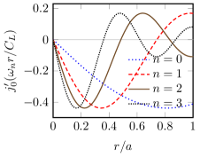
The roots can be obtained numerically for the mode frequencies . The first root corresponds to the first value of and so on. For example, choosing we find the solutions for for shown in Table 1. Using these solutions, the radial dependence for the modes, given by , is plotted in Fig. 4.
| 0.81596643669775 | 1.92853458475813 | 2.95387153514092 | 3.96577216329668 | |
| 0.62934739815975 | 1.24440286338649 | 1.42338683343041 | 1.96556466385947 | |
| 0.48514540434785 | 0.89412183542721 | 1.53070871073100 | 1.79736223921180 | |
| 0.71972992130588 | 1.18616009042197 | 1.78353164657311 | 2.15894591358743 |
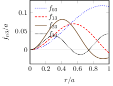
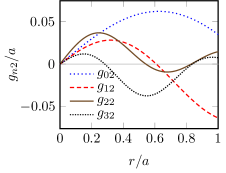
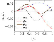
For , inserting the bulk displacement solution (61) evaluated at the surface into the boundary equation (59) results in two equations,
| (69) | ||||
| (70) | ||||
where and . The simultaneous linear equations for and have a solution if the determinant is zero,
| (71) |
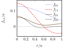
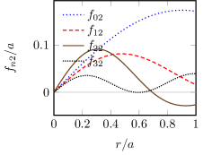
Equation (71) can be expressed in terms of and the roots can be obtained numerically. For example, for , we find the solutions for and shown in Table 1. Inserting these solutions in Eq. (69) gives the ratio of the longitudinal to the transverse parts shown in Table 2. Using these solutions, the dependence of the functions, and , on for , and is plotted in Fig. 5.
| -0.39334285456883 | 0.57828661556718 | -0.35961617280979 | 0.07851036440781 | |
| -0.68808506569504 | -0.95183672540982 | 0.55915283283423 | -1.16213124001178 | |
| -1.56275090908497 | -1.65898880431533 | 0.68019269841200 | -1.71401134238877 |

V Numerical tests
In this section, we use the analytical solutions for an elastic sphere in Sec IV to validate the numerical method presented in Sec III (in the nonrelativistic limit) and find its convergence rate.
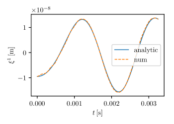
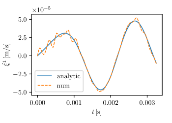
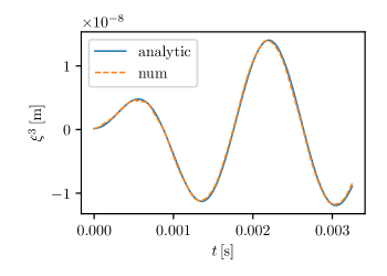
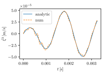
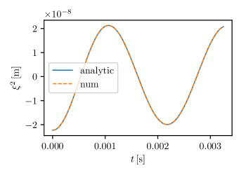
The numerical method is fully relativistic and is based on nonlinear elasticity. We set the metric equal to the Minkowski metric and choose the analytical solution to be a sum of and modes with amplitudes and and phase difference :
| (72) |
We select the material properties of the sphere such that . The amplitudes and are small compared to , and the sound speeds are small compared to the speed of light.
We use Matlab’s The MathWorks Inc. (2021) mesh generation algorithm to generate a linear tetrahedral mesh for a sphere of radius . As the mesh is refined, the total volume of tetrahedral elements converges to and we find the converged radius using the converged volume, . We use as the undeformed radius of the sphere in computing the analytical solution.
We set for all nodes at the initial time step such that their displacement from their relaxed value is equal to Eq. (72) evaluated at . We also set equal to the time derivative of Eq. (72) evaluated at . We numerically evolve the coordinates and velocities in time.
The relativistic terms in the elastic body action are of order and higher, where and is the speed of light. The nonlinear elasticity terms in the action are of order and higher. After obtaining the numerical solution we ensured that the discrepancy between the numerical and analytical solution is not due to relativistic and nonlinear elasticity effects by computing and using the numerical solution. We found that and , which makes about 16 orders of magnitude smaller than .
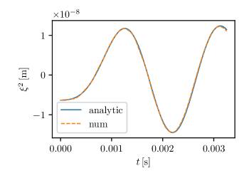
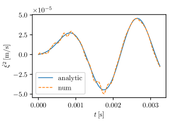
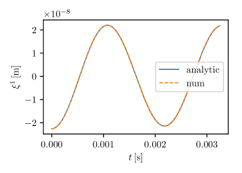
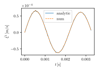
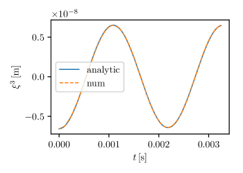
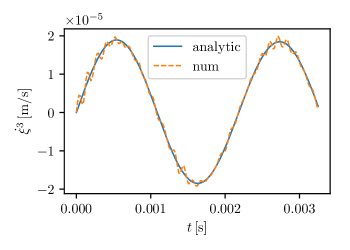
We use four mesh refinements with , where is the maximum edge length of the tetrahedral elements. Figure 6 shows the analytical and numerical displacement and velocity of the node as a function of time, for the mesh refinement with . Figure 7 shows the displacement and velocity for the node with . (The matter space coordinates are Cartesian with metric . The coordinate values are reported to four decimal places for brevity.)
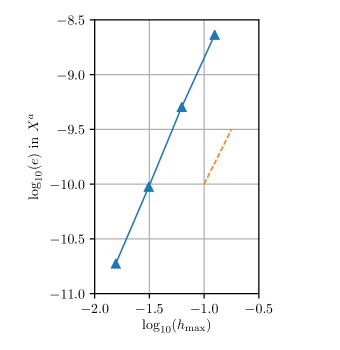
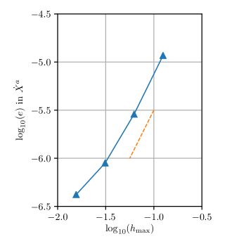
We compute the L2-norm of the error in the coordinates using
| (73) |
and similarly for the velocities. Figure 8 is the log-log plot of the L2-norm of the errors in the coordinates and velocities at the last time step as functions of . The numerical method displays second order convergence.
VI Conclusions
We have presented a second-order-convergent finite element numerical scheme for modeling extended bodies in curved spacetime using elasticity theory in general relativity. Finite elements allow a Lagrangian approach to the elastic body and provide a free surface boundary condition when formulating the numerical method. The equations of motion for the body are obtained as coupled ODEs by taking a novel approach of spatially discretizing the action. The resulting Euler-Lagrange equations are explicitly integrated in time with fourth–order Runge–Kutta, subject to a Courant condition on the time step. The numerical method can be used for bodies of any shape described by any hyperelastic potential energy function, moving through any spacetime.
Reducing to a linearized action for the hyperelastic body in the nonrelativistic limit, we reproduced the classic solutions Lamb (1881)Thorne and Blandford (2017) for radial and nonradial normal mode oscillations of an elastic sphere. These modes were then used to test the numerical code in the linearized, nonrelativistic limit. By ensuring that relativistic and nonlinear contributions are negligible, our numerical results show second-order convergence to the analytical solutions.
In a paper to follow shortly, we will apply our numerical framework to model the motion and internal dynamics of a hyperelastic sphere during tidal encounters with a Schwarzschild black hole along a quasi-parabolic orbit. Beyond that, the method presented in this paper will allow a host of investigations to be carried out on extended body interactions with spacetime curvature, including MPD spin-curvature effects on rapidly-rotating bodies and effects of higher multipole moments. Encounters could be generalized to scattering with Kerr black holes. Furthermore, the technique could be extended to include gravitational perturbations and radiation reaction effects on the finite-sized mass.
Acknowledgements.
We acknowledge the computing resources provided by North Carolina State University High Performance Computing Services Core Facility (RRID SCR_022168). We also thank Lisa L. Lowe for her assistance with porting and optimization. C.R.E. was partially supported by NSF Grant No. PHY-2110335 to the University of North Carolina–Chapel Hill.References
- Einstein and Grommer (1927) A. Einstein and J. Grommer, “Allgemeine Relativitätstheorie und Bewegungsgesetz,” Sitzungsberichte der Preussischen Akademie der Wissenschaften, Physikalisch-Mathematische Klasse 2 (1927).
- Mathisson (2010) Myron Mathisson, “Republication of: New mechanics of material systems,” General Relativity and Gravitation 42, 1011–1048 (2010).
- Papapetrou (1951) A. Papapetrou, “Spinning Test-Particles in General Relativity. I,” Proceedings of the Royal Society of London. Series A, Mathematical and Physical Sciences 209, 248–258 (1951).
- Pirani (1956) Felix AE Pirani, “On the physical significance of the riemann tensor,” Acta Physica Polonica 15, 389–405 (1956).
- Tulczyjew (1959) W Tulczyjew, “Motion of multipole particles in general relativity theory,” Acta Phys. Pol 18, 94 (1959).
- Madore (1969) John Madore, “The equations of motion of an extended body in general relativity,” Annales de l’institut Henri Poincaré. Section A, Physique Théorique 11, 221–237 (1969).
- Dixon and Bondi (1970) W. G. Dixon and Hermann Bondi, “Dynamics of extended bodies in general relativity. I. Momentum and angular momentum,” Proceedings of the Royal Society of London. A. Mathematical and Physical Sciences 314, 499–527 (1970).
- Dixon and Hewish (1970) W. G. Dixon and Antony Hewish, “Dynamics of extended bodies in general relativity - II. Moments of the charge-current vector,” Proceedings of the Royal Society of London. A. Mathematical and Physical Sciences 319, 509–547 (1970).
- Dixon and Hewish (1974) W. G. Dixon and Antony Hewish, “Dynamics of extended bodies in general relativity III. Equations of motion,” Philosophical Transactions of the Royal Society of London. Series A, Mathematical and Physical Sciences 277, 59–119 (1974).
- Kyrian and Semerák (2007) K. Kyrian and O. Semerák, “Spinning test particles in a Kerr field – II,” Monthly Notices of the Royal Astronomical Society 382, 1922–1932 (2007).
- Costa and Natário (2015) L. Filipe O. Costa and José Natário, “Center of mass, spin supplementary conditions, and the momentum of spinning particles,” Fund. Theor. Phys. 179, 215–258 (2015), arXiv:1410.6443 [gr-qc] .
- Abbott et al. (2017) B. P. Abbott et al. (LIGO Scientific Collaboration and Virgo Collaboration), “Gw170817: Observation of gravitational waves from a binary neutron star inspiral,” Phys. Rev. Lett. 119, 161101 (2017).
- De et al. (2018) Soumi De, Daniel Finstad, James M. Lattimer, Duncan A. Brown, Edo Berger, and Christopher M. Biwer, “Tidal deformabilities and radii of neutron stars from the observation of gw170817,” Phys. Rev. Lett. 121, 091102 (2018).
- Steinhoff and Puetzfeld (2012) Jan Steinhoff and Dirk Puetzfeld, “Influence of internal structure on the motion of test bodies in extreme mass ratio situations,” Phys. Rev. D 86, 044033 (2012).
- Witzany et al. (2019) Vojtěch Witzany, Jan Steinhoff, and Georgios Lukes-Gerakopoulos, “Hamiltonians and canonical coordinates for spinning particles in curved space-time,” Classical and Quantum Gravity 36, 075003 (2019).
- Hinderer (2008) Tanja Hinderer, “Tidal love numbers of neutron stars,” The Astrophysical Journal 677, 1216–1220 (2008).
- Harte (2020) Abraham I. Harte, “Extended-body motion in black hole spacetimes: What is possible?” Phys. Rev. D 102, 124075 (2020), arXiv:2011.00110 [gr-qc] .
- Chamel and Haensel (2008) Nicolas Chamel and Pawel Haensel, “Physics of neutron star crusts,” Living Reviews in relativity 11, 1–182 (2008).
- Camisassa, María E. et al. (2019) Camisassa, María E., Althaus, Leandro G., Córsico, Alejandro H., De Gerónimo, Francisco C., Miller Bertolami, Marcelo M., Novarino, María L., Rohrmann, René D., Wachlin, Felipe C., and García-Berro, Enrique, “The evolution of ultra-massive white dwarfs,” A&A 625, A87 (2019).
- Gundlach et al. (2011) Carsten Gundlach, Ian Hawke, and Stephanie Jeanne Erickson, “A conservation law formulation of nonlinear elasticity in general relativity,” Classical and Quantum Gravity 29 (2011).
- Alho et al. (2022) Artur Alho, José Natário, Paolo Pani, and Guilherme Raposo, “Compact elastic objects in general relativity,” Phys. Rev. D 105, 044025 (2022).
- Alho et al. (2023) Artur Alho, José Natário, Paolo Pani, and Guilherme Raposo, “Spherically symmetric elastic bodies in general relativity,” arXiv e-prints , arXiv:2307.03146 (2023).
- Karlovini and Samuelsson (2003) Max Karlovini and Lars Samuelsson, “Elastic stars in general relativity: I. Foundations and equilibrium models,” Classical and Quantum Gravity 20, 3613 (2003).
- Karlovini et al. (2004) Max Karlovini, Lars Samuelsson, and Moundheur Zarroug, “Elastic stars in general relativity: II. Radial perturbations,” Classical and Quantum Gravity 21, 1559 (2004).
- Karlovini and Samuelsson (2004) Max Karlovini and Lars Samuelsson, “Elastic stars in general relativity: III. Stiff ultrarigid exact solutions,” Classical and Quantum Gravity 21, 4531 (2004).
- Karlovini and Samuelsson (2007) Max Karlovini and Lars Samuelsson, “Elastic stars in general relativity: IV. Axial perturbations,” Classical and Quantum Gravity 24, 3171 (2007).
- Brown (2021) J David Brown, “Elasticity theory in general relativity,” Classical and Quantum Gravity 38, 085017 (2021).
- Misner et al. (1973) C.W. Misner, K.S. Thorne, and J.A. Wheeler, Gravitation (W. H. Freeman, 1973).
- Herglotz (1911) G. Herglotz, “Über die mechanik des deformierbaren körpers vom standpunkte der relativitätstheorie,” Annalen der Physik 341, 493–533 (1911).
- DeWitt (1962) Bryce S. DeWitt, “The quantization of geometry,” in Gravitation: An Introduction to Current Research (Wiley, 1962).
- Carter and Quintana (1972) B. Carter and H. Quintana, “Foundations of general relativistic high-pressure elasticity theory,” Proceedings of the Royal Society of London. Series A, Mathematical and Physical Sciences 331, 57–83 (1972).
- Kijowski and Magli (1992) Jerzy Kijowski and Giulio Magli, “Relativistic elastomechanics as a lagrangian field theory,” Journal of Geometry and Physics 9, 207–223 (1992).
- Beig and Schmidt (2003) Robert Beig and Bernd G. Schmidt, “Relativistic elasticity,” Classical and Quantum Gravity 20, 889–904 (2003), arXiv:gr-qc/0211054 [gr-qc] .
- Beig and Schmidt (2017) Robert Beig and Bernd G Schmidt, “Celestial mechanics of elastic bodies II,” Classical and Quantum Gravity 34, 085001 (2017).
- Beig (2023) Robert Beig, “Relativistic elasticity II,” Classical and Quantum Gravity 40, 084001 (2023), arXiv:2303.05870 [gr-qc] .
- Lanczos (1949) C. Lanczos, The Variational Principles of Mechanics, Heritage Series (University of Toronto Press, 1949).
- Landau and Lifshitz (1951) L.D. Landau and E.M. Lifshitz, The Classical Theory of Fields (Pergamon, Oxford, 1951).
- Bower (2009) A.F. Bower, Applied Mechanics of Solids (CRC Press, Boca Raton, 2009).
- (39) P.A. Kelly, Mechanics Lecture Notes: An introduction to Solid Mechanics, available from http://homepages.engineering.auckland.ac.nz/ pkel015/SolidMechanicsBooks/index.html.
- Piola (1832) G. Piola, “La meccanica de’ corpi naturalmente estesi: trattata col calcolo delle variazioni,” in Opuscoli atematici e fisici di diversi autori (Giusti, 1832) pp. 201–236.
- Kirchhoff (1852) G Kirchhoff, “Über die gleichungen des gleichgewichtes eines elastischen körpers bei nicht unendlich kleinen verscheibungen seiner theile,” Sitzsber. Akad. Wiss. Wien 9, 762 (1852).
- Brown and Marolf (1996) J. David Brown and Donald Marolf, “Relativistic material reference systems,” Phys. Rev. D 53, 1835–1844 (1996).
- Li et al. (2017) Zhilin Li, Zhonghua Qiao, and Tao Tang, “Finite element methods for 1d boundary value problems,” in Numerical Solution of Differential Equations: Introduction to Finite Difference and Finite Element Methods (Cambridge University Press, 2017) p. 135–157.
- The MathWorks Inc. (2021) The MathWorks Inc., “Partial Differential Equation Toolbox,” (2021).
- Karypis and Kumar (1997) George Karypis and Vipin Kumar, “Metis—a software package for partitioning unstructured graphs, partitioning meshes and computing fill-reducing ordering of sparse matrices,” (1997).
- Hughes (2012) T.J.R. Hughes, The Finite Element Method: Linear Static and Dynamic Finite Element Analysis, Dover Civil and Mechanical Engineering (Dover Publications, 2012).
- Mooney (2004) M. Mooney, “A Theory of Large Elastic Deformation,” Journal of Applied Physics 11, 582–592 (2004), https://pubs.aip.org/aip/jap/article-pdf/11/9/582/7905927/582_1_online.pdf .
- Ogden and Hill (1972) Raymond William Ogden and Rodney Hill, “Large deformation isotropic elasticity – on the correlation of theory and experiment for incompressible rubberlike solids,” Proceedings of the Royal Society of London. A. Mathematical and Physical Sciences 326, 565–584 (1972).
- Lamb (1881) Horace Lamb, “On the vibrations of an elastic sphere,” Proceedings of the London Mathematical Society s1-13, 189–212 (1881).
- Love (1892) A.E.H. Love, A Treatise on the Mathematical Theory of Elasticity, A Treatise on the Mathematical Theory of Elasticity No. v. 1 (University Press, 1892).
- Thorne and Blandford (2017) K. S. Thorne and R. D. Blandford, Modern Classical Physics: Optics, Fluids, Plasmas, Elasticity, Relativity, and Statistical Physics (Princeton University Press, 2017).