Controlling Majorana hybridization in magnetic chain-superconductor systems

Abstract

We propose controlling the hybridization between Majorana zero modes at the ends of magnetic adatom chains on superconductors by an additional magnetic adatom deposited close by. By tuning the additional adatom’s magnetization, position, and coupling to the superconductor, we can couple and decouple the Majorana modes as well as control the ground state parity. The scheme is independent of microscopic details in ferromagnetic and helical magnetic chains on superconductors with and without spin-orbit coupling, which we show by studying their full microscopic models and their common low-energy description. Our results show that scanning tunneling microscopy and electron spin resonance techniques are promising tools for controlling the Majorana hybridization in magnetic adatoms-superconductor setups, providing a basis for Majorana parity measurements, fusion, and braiding techniques.

I Introduction

Majorana zero modes (MZMs) are non-Abelian quasiparticles that are their own anti-particles and have been subject to intense research in condensed matter physics due to their exotic properties and potential application in fault-tolerant topological quantum computing [1, 2, 3, 4, 5, 6, 7, 8]. Among the most promising platforms for realizing MZMs are systems based on topological insulators  [9, 10, 11], fractional quantum Hall systems [12, 13, 14], ultracold atoms [15, 16, 17], semiconducting nanowires [18, 19, 20, 21], planar Josephson junctions [22, 23, 24, 25] and magnetic adatoms chain deposited on a superconductor [26, 27, 28, 29, 30, 31, 32, 33, 34, 35]. While there has been immense theoretical and experimental progress, especially in semiconducting nanowires-superconducting hybrid structures, the short nanowire length and disorder in these systems is a major challenge in the search of MZMs [36]. Progress with this platform demands clean systems with nanowires much longer than the coherence length of the superconductor, which is difficult with present technology. In the search for alternatives, magnetic adatoms on a superconductor have garnered a lot of interest where MZMs could be directly probed using a scanning tunneling microscope [30, 37, 38, 39]. Here, a single magnetic adatom deposited on a superconductor induces a spin-polarized Yu-Shiba-Rusinov (YSR) state within the superconducting gap [40, 41, 42, 43]. When a chain of such magnetic adatoms is deposited on a superconductor, the spin-polarized YSR states from the individual magnetic adatoms overlap to form a nondegenerate Shiba band which leads to an effective $p$-wave superconducting gap in the chain’s electronic spectrum when an effective spin-orbit coupling is present. This $p$-wave superconductor formed by the magnetic adatom chain is topologically nontrivial, hosting a MZM at each end. Two salient frameworks to realize this proposal are a chain of magnetic adatoms with helical magnetization on an $s$-wave superconductor [26, 27, 28, 29, 44, 45, 46, 47, 48, 49, 50, 51, 52, 53, 54] and a chain of ferromagnetic adatoms deposited on an $s$-wave superconductor with spin-orbit coupling [32, 30, 31, 37, 55, 33, 34, 35, 56].

Several STM experiments have reported zero-bias peaks in differential conductance measurements on magnetic chain-superconductor systems, which have been interpreted in terms of MZMs  [30, 37, 34, 35]. However, zero-bias peaks can also stem from the trivial in-gap states in the magnetic chain [57, 58]. In fact, it has been established across realistic platforms proposed for creating MZMs that the observed zero-bias conductance peaks can have alternative explanations [59, 60, 61, 57], a development that has opened up a debate about whether the MZMs have been observed in reported experiments. Unambiguous verification of zero-bias peaks as MZM signals involves measurements exploring their non-Abelian properties, such as fusion and braiding behavior, which are not shared by trivial in-gap states, or via cross-correlation shot noise measurements [62]. While there is an abundance of such proposals in semiconducting platforms, see Refs. [63, 64, 65, 66, 67, 68, 69, 70] for examples, the adatoms route has received much less attention  [53, 71]. This can partly be attributed to the rigidity of this platform since, once fabricated, the system parameters are difficult to manipulate externally, which is a prerequisite for quantum information processing. To carry out non-Abelian experiments, it is imperative to have a high-quality, time-dependent control over the hybridization between MZMs, resulting in their coupling and decoupling, as a first step towards experiments revealing their non-Abelian character.

In this paper, we propose a generic method to control and shield, i.e., switch off, the hybridization of MZMs in magnetic chain-superconductor systems via a single additional magnetic adatom. We consider two chains of magnetic adatoms on an $s$-wave superconductor with a single magnetic adatom in between such that there is finite overlap between the MZMs at the ends of the magnetic chains in the topological phase and the YSR state induced by the single magnetic adatom. We find a model-independent strong tunability of the MZMs hybridization energy by changing the single adatom’s magnetic orientation, its distance from the magnetic chains and its coupling to the superconductor. Here, the control of the parameters of the single magnetic adatom can, in principle, be achieved using electron spin resonance-scanning tunneling microscopy (ESR-STM) techniques [72, 73, 74, 75], see Sec. IV for details. Remarkably, we find that these parameters tune the MZMs hybridization through a vast range of values: between strongly hybridized MZMs and zero, where the MZMs are perfectly shielded from each other. The complete shielding of the MZMs occurs for fine-tuned parameters that mark a phase transition between regions with different ground state parity. We show that our results are general and not model specific, which we demonstrate by the general low-energy model and specific well-studied microscopic models of helical and ferromagnetic adatoms chains in both continuum and lattice superconductor models. As an overarching theme, our results show a wide variability of the MZMs hybridization with the orientation of the single magnetic adatom, which is accessible with current experimental techniques. The control of MZMs hybridization is an essential prerequisite for Majorana fusion and braiding experiments. Thus, our work is a step towards realizing these MZMs prospects and opens a novel experimentally realizable research direction in the magnetic chain-superconductor platform. Moreover, the shielding effect can be used to decouple strongly hybridized Majorana modes, also called precursors of Majorana modes, which were observed in short magnetic chains [56]. Furthermore, changes in the ground state parity imply control over the occupation of the ground state of the system, which is essential for initialization in parity-based Majorana correlation measurements, where perturbing one of the chains induces measurable parity oscillation in the other chain [76, 77, 78]. Our results enhance the understanding of the behavior of MZMs and inspire future experiments for probing non-Abelian properties of MZMs and employing them in fault-tolerant quantum computing.

The remainder of the paper is organized as follows: In Sec. II, we introduce the system to control the MZMs hybridization and present a general low-energy model to analytically evaluate the effective Majorana hybridization. We show the possible decoupling of the MZMs due to the overlap with the YSR state from the single magnetic adatom and also provide an analysis of the change in the ground state parity. In Sec. III, we show the generality of the control of MZMs hybridization by addressing three experimentally relevant physical realizations. We first present general analytical results for continuum superconductors in Sec. III.1, and then consider helically ordered magnetic chains on a conventional $s$-wave superconductor and ferromagnetic ordered chains on an $s$-wave superconductor with non-zero spin-orbit coupling both in the continuum limit, in Sec. III.1.1 and Sec. III.1.2, respectively. In Sec. III.2, we consider a ferromagnetic chain on a square lattice superconductor with finite spin-orbit coupling. In Sec. IV, we discuss a possible experimental protocol for the proposed setup. Finally, we give concluding remarks in Sec. V, where we discuss possible future experiments achievable with our proposal, including manipulating and decoupling precursors of Majorana modes, and a possible method to control the Majorana hybridization using the dynamics of the single magnetic adatom.

II The System

We consider a setup with two chains, left and right, consisting of $N_{\rm L}$ and $N_{\rm R}$ magnetic adatoms, respectively, that are deposited on an $s$-wave superconductor and separated by a distance $R$ from each other, see Fig. 1, where Fig. 1(a) and (b) depict ferromagnetic chains and helical magnetic chain on an s-wave superconductor with finite and vanishing Rashba spin-orbit coupling, respectively. In addition, a single magnetic adatom (blue sphere), with magnetic orientation $\boldsymbol{S}_{\rm S}=\boldsymbol{S}_{\rm S}(\sin\theta_{\rm S}\cos\phi_{\rm S},\sin\theta_{\rm S}\sin\phi_{\rm S},\cos\theta_{\rm S})$, where $\theta_{\rm S}$ and $\phi_{\rm S}$ are the polar and azimuthal angle, respectively, is placed at position $\boldsymbol{R}_{\rm S}=(x_{\rm S},y_{\rm S},z_{\rm S})$ relative to the right end of the left chain, inducing a YSR state of energy $\epsilon_{\rm S}(\phi_{\rm S},\leavevmode\nobreak\ \theta_{\rm S})$ centered at this position. The chains are in the topologically non-trivial phase, each accommodating a pair of MZMs at its ends which are represented by $\gamma$-operators, orange density of states in Fig. 1. The magnetic chains are long enough to avoid overlap of the inner MZMs, $\gamma_{\rm L}$ and $\gamma_{\rm R}$, with the outer MZMs, $\gamma_{\rm L}^{\prime}$ and $\gamma_{\rm R}^{\prime}$. Yet, there is a finite bare hybridization energy, $\epsilon_{\rm M}\left(R\right)$, between the inner MZMs, $\gamma_{\rm L}$ and $\gamma_{\rm R}$, leading to the formation of a non-local fermion with energy $\epsilon_{\rm M}$.

Figure 1: Realizations of the system. (a) Two ferromagnetic chains with the left and right chain consisting of $N_{\rm L}$ and $N_{\rm R}$ adatoms, respectively, on an $s$-wave superconductor, separated by a distance $R$. An additional adatom (blue) with magnetic orientation $\boldsymbol{S}_{\rm S}(\phi_{\rm S},\leavevmode\nobreak\ \theta_{\rm S})$ is placed at distance $\boldsymbol{R}_{\rm S}$ from the left chain. In the topologically nontrivial phase, the MZMs $\gamma_{\rm L}^{\prime}$, $\gamma_{\rm L}$, $\gamma_{\rm R}$, and $\gamma_{\rm R}^{\prime}$ reside at the chains’ ends, whose density of states is shown in orange. Inset: schematic dependence of the effective MZMs hybridization energy $E_{\rm M}$ and the effective YSR energy $E_{\rm S}$ on $\phi_{\rm S}$, $\Delta_{\rm t}$ denotes the topological gap. (b) Same as (a) but with helically magnetized adatoms on an $s$-wave superconductor with vanishing spin-orbit coupling. The STM tip (green) can be used to control the parameters of the single magnetic adatom by applying a time-dependent electric field.

The superconductor mediates a finite coupling between the inner MZMs and the YSR state at $\boldsymbol{R}_{\rm S}$ which effectively modifies both $\epsilon_{\rm M}\left(R\right)$ and $\epsilon_{\rm S}\left(\theta_{\rm S},\phi_{\rm S}\right)$ to new values $E_{\rm M}\left(R_{\rm S},\theta_{\rm S},\phi_{\rm S},\epsilon_{\rm S},\epsilon_{\rm M},R\right)$ and $E_{\rm S}\left(R_{\rm S},\theta_{\rm S},\phi_{\rm S},\epsilon_{\rm S},\epsilon_{\rm M},R\right)$, respectively. A typical dependence of $E_{\rm M}$ and $E_{\rm S}$ on $\phi_{\rm S}$ is shown in the inset of Fig. 1(a), explained in detail in Sec. III. It should be noted that $E_{\rm M}$ and $E_{\rm S}$ correspond to hybridized Majorana and YSR states with density of states at both original states’ positions.

Assuming that $|\epsilon_{\rm M}|$ and $|\epsilon_{\rm S}|$ are much smaller than the topological gap of the Shiba bands $\Delta_{\rm t}$, all systems discussed in this work share the same low-energy limit, where only the in-gap states in the central region of the setup are relevant, including the overlapping inner MZMs $\gamma_{L}$ and $\gamma_{R}$, and the single magnetic adatom’s YSR state, see Fig. 1. We ignore the outer MZMs because they decouple from the central region for sufficiently long chains. After integrating out the superconductor and the Shiba bands of the chains, the effective low-energy Hamiltonian for the $\gamma_{L}$-YSR-$\gamma_{R}$ system is

$$H_{\rm eff}=\frac{i}{2}\epsilon_{\rm M}\gamma_{\rm L}\gamma_{\rm R}+\epsilon_{\rm S}d^{\dagger}d+\left[t_{\rm L}d^{\dagger}\gamma_{\rm L}+t_{\rm R}d^{\dagger}\gamma_{\rm R}+\rm{h.c.}\right],$$ (1)

where $d^{\dagger}$ creates an electron in the YSR state, $t_{\rm L/R}=t_{\rm L/R}\left(R_{\rm S},\theta_{\rm S},\phi_{\rm S},\epsilon_{\rm S},\epsilon_{\rm M},R\right)$ is the coupling amplitude between the YSR state and the MZM $\gamma_{\rm L/R}$ with $\{\gamma_{i},\gamma_{j}\}=2\delta_{ij}$. The Hamiltonian in Eq. (1) preserves particle-hole symmetry, breaks time-reversal symmetry, and thus belongs to the topological class $D$ in the Cartan-Altland-Zirnbauer scheme for topological superconductors [79, 80].

To access the effective MZM and YSR energies, we express the Hamiltonian in Eq. (1) in a full fermionic basis by $f=\frac{1}{2}(\gamma_{\rm L}+i\gamma_{\rm R})$, where $f^{\dagger}$ is the creation operator of the non-local fermion with energy $\epsilon_{\rm M}$. The four single-particle eigenvalues are,

$$\begin{split}E_{\rm{S}}&=\pm\tfrac{1}{2}\left[\sqrt{\epsilon_{+}^{2}+4|t_{+}|^{2}}+\sqrt{\epsilon_{-}^{2}+4|t_{-}|^{2}}\right]\\ E_{\rm{M}}&=\pm\tfrac{1}{2}\left[\sqrt{\epsilon_{+}^{2}+4|t_{+}|^{2}}-\sqrt{\epsilon_{-}^{2}+4|t_{-}|^{2}}\right],\end{split}$$ (2)

where $t_{\pm}=t_{\rm L}\pm it_{\rm R}$ and $\epsilon_{\pm}=\epsilon_{\rm M}\pm\epsilon_{\rm S}$. The two solutions with larger energy value, $|E_{\rm S}|$, are the effective YSR energies, while the two solutions with smaller energy value, $|E_{\rm M}|$, are the effective MZM hybridization energies. The localization of the corresponding states of $E_{\rm M/S}$ strongly depends on the parameters of the single magnetic adatom, see Appendix A for details. The effective energies are unchanged under the adiabatic exchange of $\gamma_{\rm L}$ and $\gamma_{\rm R}$, which leads to $\gamma_{\rm L}\rightarrow-\gamma_{\rm R}$ and $\gamma_{\rm R}\rightarrow\gamma_{\rm L}$ [3]. This implies $\epsilon_{\rm M}\rightarrow\epsilon_{\rm M},\,t_{\rm L}\rightarrow t_{\rm R},\,t_{\rm R}\rightarrow-t_{\rm L}$, leaving Eq. (2) invariant. Also, swapping the labels R and L in Eq. (1), leaves Eq. (2) unchanged since $\epsilon_{\rm M}\rightarrow-\epsilon_{\rm M}\implies\epsilon_{\pm}\rightarrow-\epsilon_{\pm}$, and all other parameters are unaffected.

We are most interested in a vanishing effective Majorana hybridization $E_{\rm M}$. Importantly, in symmetry class $D$, this corresponding zero-energy crossing of the Majorana level is generally accompanied by a change in the fermion ground state parity, which is conveniently described by $P=\operatorname{sgn}\left(\rm Pf\left[\tilde{H}_{\rm eff}\right]\right)$, i.e., the sign of the Pfaffian of $\tilde{H}_{\rm eff}$, which is obtained by writing $H_{\rm eff}$ in Majorana basis [81, 26, 82]. We hence find that the effective Majorana hybridization crosses zero and the ground state parity changes only at

$$\Im[t_{\rm R}]\Re[t_{\rm L}]-\Im[t_{\rm L}]\Re[t_{\rm R}]=\dfrac{\epsilon_{\rm M}\epsilon_{\rm S}}{4},$$ (3)

see Appendix B for details. One scenario to satisfy Eq. (3) is when one of $t_{\rm L}$ and $t_{\rm R}$ is zero or both are real (both of which give $|t_{-}|=|t_{+}|$) and $\epsilon_{\rm S}$ or $\epsilon_{\rm M}$ is zero. The investigation of more general possibilities, when both sides of Eq. (3) are finite, requires knowledge about the parameters in Eq. (3), which depend on the microscopic model, see inset in Fig. 1(a) for a representative dependence of the effective Majorana hybridization on the magnetic orientation of the single adatom. An important implication of the above result is that the parity switching, which can be determined through charge sensing [76, 83, 84, 85], can serve as a tool for tracking the MZMs shielding. Furthermore, controlling the ground state parity is essential in parity-based measurements of Majorana correlations [76]. Here, one can perturb one of the chains or control its parity through the parameters of the single adatom while simultaneously measuring the parity of the second chain, which is expected to change due to the entanglement between the MZMs.

While the control of the Majorana hybridization and the accompanying parity switching are general for the Majorana setups in Fig. 1, the microscopic details of the systems are required in order to examine the dependence of the MZMs hybridization on the control parameters of the YSR state. We explore the experimentally relevant realizations in Fig. 1 for this purpose. In what follows, we, therefore, investigate the widely studied arrangements of magnetic adatoms on superconductors with helical magnetization and the ones with ferromagnetic ordering.

III Physical realizations

In this Section, we describe in detail physical realizations of magnetic chain-superconductor systems and show explicitly the dependence of the hybridization of MZMs on the control parameters. In Sec. III.1, we consider continuum models for the superconducting substrates, derive general expressions for $t_{\rm L/R}$, and subsequently demonstrate the control of Majorana hybridization for helical and ferromagnetic chains. In Sec. III.2, we consider ferromagnetic chains on a lattice superconductor and show that the model yields the same results as the former, demonstrating the universality of our findings.

III.1 Continuum models for the substrate superconductor

We first discuss models where the superconducting substrate is incorporated by continuous fields. In the dilute adatom limit, $k_{\rm F}a\gg 1$, where $k_{\rm F}$ is the Fermi wave number of the superconducting substrate, an effective Hamiltonian that captures the basic physics of this setup can be written in the basis of the YSR states induced by the individual adatoms in the chain if the energy of each YSR state is close to the Fermi energy [28, 31]. Following Refs. [28, 31], we apply the approach to the setup in Fig. 1(b) and obtain the effective Hamiltonian as,

$$\begin{split}&\mathcal{H}=\mathcal{H}_{\rm L}+\mathcal{H}_{\rm R}+\mathcal{H}_{\rm LR}+\mathcal{H}_{\rm d}\\ &\mathcal{H}_{\rm L}=\sum_{m=1}^{N_{L}}\sum_{n=1}^{N_{L}}b_{m}^{\dagger}\left[\epsilon_{0}\delta_{mn}+\left(1-\delta_{mn}\right)h_{mn}\right]b_{n}+b_{m}\left(1-\delta_{mn}\right)\Delta_{mn}b_{n}+{\rm h.c.},\\ &\mathcal{H}_{\rm R}=\sum_{m=N_{L}+R/a}^{N_{L}+N_{R}+R/a}\sum_{n=N_{L}+R/a}^{N_{L}+N_{R}+R/a}b_{m}^{\dagger}\left[\epsilon_{0}\delta_{mn}+\left(1-\delta_{mn}\right)h_{mn}\right]b_{n}+b_{m}\left(1-\delta_{mn}\right)\Delta_{mn}b_{n}+{\rm h.c.},\\ &\mathcal{H}_{\rm LR}=\sum_{m=1}^{N_{L}}\sum_{n=N_{L}+R/a}^{N_{L}+N_{R}+R/a}\left[h_{mn}b_{m}^{\dagger}b_{n}+b_{m}\left(1-\delta_{mn}\right)\Delta_{mn}b_{n}\right]+{\rm h.c.},\\ &\mathcal{H}_{\rm S}=\epsilon_{\rm S}d^{\dagger}d+\left[\sum_{m=1}^{N_{L}}\left(h_{N_{L}+\frac{R_{\rm S}}{a},m}d^{\dagger}+\Delta_{N_{L}+\frac{R_{\rm S}}{a},m}d\right)+\sum_{m=N_{L}+R/a}^{N_{L}+N_{R}+R/a}\left(h_{N_{L}+\frac{R_{\rm S}}{a},m}d^{\dagger}+\Delta_{N_{L}+\frac{R_{\rm S}}{a},m}d\right)\right]b_{m}+{\rm h.c.},\end{split}$$ (4)

where $b_{m}^{\dagger}$ creates an electron with energy $\epsilon_{0}$ in the YSR state at site $m=\left(x_{m},y_{m},z_{m}\right)$ in the chain and $d^{\dagger}$ creates an electron with energy $\epsilon_{\rm S}$ in the YSR state at the position of the single magnetic adatom. Here, $\mathcal{H}_{\rm LR}$ couples the YSR states in the left chain to those in the right chain and vice versa while the second term of $\mathcal{H}_{\rm S}$ couples the YSR state from the single magnetic adatom to all YSRs states in the left and right chains. In the general form, the long-range hopping $h_{mn}$ and order parameters $\Delta_{mn}$ are given by [31, 86],

$$h_{mn} =h_{mn}^{(0)}\langle\uparrow m\mid\uparrow n\rangle+h_{mn}^{(1)}\left\langle\uparrow m\left|i\sigma_{y}\right|\uparrow n\right\rangle,$$ (5)

$$\Delta_{mn} =\Delta_{mn}^{(0)}\langle\uparrow m\mid\downarrow n\rangle+\Delta_{mn}^{(1)}\left\langle\uparrow m\left|i\sigma_{y}\right|\downarrow n\right\rangle,$$

where $\sigma_{\nu}$ is the $\nu$-Pauli matrix, and $h_{mn}^{(1)}$ and $\Delta_{mn}^{(1)}$ are material-dependent constants that vanish when spin-orbit coupling is absent in the superconductor. Here,

$$|\uparrow m\rangle=\left(\cos\left(\theta_{m}/2\right)e^{-i\phi_{\rm m}/2},\sin\left(\theta_{m}/2\right)e^{i\phi_{\rm m}/2}\right)^{T},$$

$$|\downarrow m\rangle=\left(\sin\left(\theta_{m}/2\right)e^{-i\phi_{\rm m}/2},-\cos\left(\theta_{m}/2\right)e^{i\phi_{\rm m}/2}\right)^{T},$$

are the spinors corresponding to the magnetic orientations of the adatoms in the chains at position $\boldsymbol{r}_{m}$, which is denoted by $S\left(\sin\theta_{m}\cos\phi_{m},\sin\theta_{m}\sin\phi_{m},\cos\theta_{m}\right)$, where $S$ is the magnitude of the spin and $\theta_{m}$ and $\phi_{m}$ are the polar and azimuthal angles, respectively [28, 46, 31]. Due to the phase factors in $h_{mn}$ and $\Delta_{mn}$ in Eq. (5), $\mathcal{H}_{\rm L}$ and $\mathcal{H}_{\rm R}$ in Eq. (4) break time-reversal symmetry but preserve particle-hole symmetry, thus, the chains are class $D$ topological superconductors [79, 87, 88, 80] like the effective low-energy model in Eq. (1).

While the bare Majorana hybridization, $\epsilon_{\rm M}$, depends only on the distance R between the chains and the material-specific details, the low-energy coupling $t_{\rm L/R}$ on the other hand depends also on the parameters associated with the single magnetic adatom. We find that $t_{\rm L/R}$ have separable dependencies on the magnetic adatom’s spin orientation and the remaining parameters. By using Eqs. (4) and (5) with Eq. (1), (see Appendix C for details) we obtain the general form of the couplings,

$$t_{\rm L/R}=e^{i\frac{\phi_{\rm S}}{2}}\cos\left(\frac{\theta_{\rm S}}{2}\right)\,F_{L/R}+e^{-i\frac{\phi_{\rm S}}{2}}\sin\left(\frac{\theta_{\rm S}}{2}\right)\,G_{\rm L/R},$$ (6)

where the functions $G_{\rm L/R}=G_{\rm L/R}\left(R_{\rm S}\right)$ and $F_{\rm L/R}=F_{\rm L/R}\left(R_{\rm S}\right)$ contain the microscopic details of the superconductor and magnetic chain. Here, $F_{L/R}$ can be obtained from $G_{L/R}$ by flipping the direction of every spin of each chain, $F_{L/R}(\phi_{m},\theta_{m})=G_{L/R}(-\phi_{m},\pi-\theta_{m})$. Equation (6) is valid for all magnetic adatoms chain-superconductor systems in the dilute and deep Shiba limits.

Next, we present two specific continuum models of our setup and demonstrate the control of the Majorana hybridization.

III.1.1 Helically magnetized chains on a conventional $s$-wave superconductor

A well-studied model is the helical arrangement of the magnetic adatoms chain on the SC due to the RKKY interactions [89, 28, 53]. Such a spin structure was found for iron adatoms on the surface of superconducting rhenium [34].

In the absence of spin-orbit coupling, corresponding to $h_{mn}^{(1)}=\Delta_{mn}^{(1)}=0$ in Eq. (5), analytical zero energy Majorana solutions of $\mathcal{H}_{\rm L}$ and $\mathcal{H}_{\rm R}$ can be found in the vicinity of the Bragg point, $k_{h}=k_{\rm F}$, where $k_{h}=2\pi\chi$ is the wave vector corresponding to the periodicity of the helix $\chi$ [29]. We first focus on the Bragg point for building up a physical understanding. We have explored deviations from this point numerically and found no qualitative difference when the system remains in the topologically nontrivial phase. Following Ref. [28], we consider an in-plane helical magnetization in the chains, which corresponds to setting $\theta_{m}=\pi/2$. We further specify the helical structure for the left (right) chain as $\phi_{{\rm L},m}=-2k_{h}am$ $\left(\phi_{{\rm R},m}=2k_{h}am\right)$, and we fix $m=0$ at the inner ends of the chains, which are both oriented in the $x$ direction. For analytical tractability, we consider the semi-infinite limit of both chains such that the outer MZMs, $\gamma_{\rm L/R}^{\prime}$, are at infinity. For this case, we find that $G_{\rm L}(R_{\rm S})=-iF_{\rm L}^{*}(R_{\rm S})$ and $G_{\rm R}(R_{\rm S})=iF_{\rm R}^{*}(R_{\rm S})$, see Appendix C.1. Using this result and the Majorana solutions of $\mathcal{H}_{\rm L}$ and $\mathcal{H}_{\rm R}$ [29], we find the effective low-energy parameters in Eq. (1), see Appendix D, as

$$\begin{split}&\epsilon_{\rm M}=\frac{iB^{2}}{\Delta k_{\rm F}a}\sum_{\begin{subarray}{c}w=1,2\\ \zeta=\pm\end{subarray}}\zeta e^{-A_{\zeta}}\frac{{}_{2}F_{1}\left(w,\frac{R}{a}+w-1;\frac{R}{a}+w;e^{A_{\zeta}}\right)}{\frac{R}{a}+w-1},\\ &t_{\rm L}=t_{\rm L}\left(F_{\rm L}\rightarrow G,G_{\rm L}\rightarrow-iG^{*}\right),\\ &t_{\rm R}\left(R_{\rm S},\phi_{\rm S},\theta_{\rm S}\right)=t_{\rm L}^{*}\left(R-R_{\rm S},-\phi_{\rm S},\theta_{\rm S}\right),\\ &G=\frac{Be^{-\left[ik_{\rm F}R_{\rm S}+\frac{R_{\rm S}}{\xi_{\rm sc}}+i\frac{\pi}{4}\right]}}{2k_{\rm F}R_{\rm S}}\ {}_{2}F_{1}\left(1,\frac{R_{\rm S}}{a};\frac{R_{\rm S}}{a}+1;e^{A_{-}}\right).\end{split}$$ (7)

Here, $B^{2}=\frac{\left(1-\beta^{2}\right)\Delta^{2}}{2}$, $\beta=\frac{e^{a/\xi_{\rm sc}}\sin\left(k_{F}a\epsilon_{0}/\Delta\right)}{\sin\left(2k_{F}a+k_{F}a\epsilon_{0}/\Delta\right)}$, $A_{\zeta}=-\frac{a}{\xi_{\rm sc}}+\ln{(\beta)+i\zeta 2k_{\rm F}a}$, ${}_{2}F_{1}$ is the ordinary hypergeometric function and $\xi_{\rm sc}$ is the superconducting coherence length of the substrate. For the effective model parameters in Eq. (7), we use a 3D bulk superconductor in the model. If the inter-chain distance $R$ is large or the single magnetic adatom is far from the chains, the effective model parameters are small and can be represented by their asymptotic form, see Appendix E.

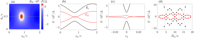
Figure 2: Majorana hybridization at the Bragg point of a chain of helically-oriented planar spins on an $s$-wave superconductor (continuum model). (a) The effective Majorana energy multiplied with the ground state parity, $E_{\rm M}\cdot P$, as a function of the orientation of the single magnetic adatom $\phi_{\rm S}$ and $\theta_{\rm S}$ for bare adatom energy $\epsilon_{\rm S}=0.002\Delta$ and a distance from the left chain $R_{\rm S}=8a$. The red and blue regions have opposite parity, while the MZMs are decoupled in between. (b) Linecut along the dashed green line in (a). (c) Hybridization as a function of the YSR energy $\epsilon_{\rm S}$ at $\phi_{\rm S}=\pi$, and (d) as a function of the distance from the left chain $R_{\rm S}$ at $\phi_{\rm S}=0$. Here, $R_{\rm S}$ is plotted in steps of the inter magnetic adatom distance, $a$, in the chains. In all panels, we set the distance between the chains $R=20a$, the bare energy of the magnetic adatoms of the chains $\epsilon_{\rm 0}=0.005\Delta$, and the superconducting coherence length $\xi_{\rm sc}=15a$.

Combining Eqs. (7) and (2), we next track both the shielding effect and the tuning of the Majorana hybridization. First, we focus on controlling the Majorana hybridization and its shielding with the single adatom’s magnetic orientation, which is the parameter that can be altered fastest in an experiment, being adaptable without changing the positions of the adatoms. Notably, the effective Majorana hybridization, $E_{\rm M}$, is tuned through a wide range of values, see Fig. 2(a), where the blue and the red region denote parameter regimes of different ground state parity. Remarkably, at the boundary between these parameter regions, the MZMs are completely decoupled, $E_{\rm M}=0$, as described by Eq. (3). Such a parity switch, seen in the change in the sign of $E_{\rm M}$, around this region confirms the zero-energy crossing of the MZMs.

To further understand the Majorana shielding effect for the model, we consider the case where $\theta_{\rm S}=\pi/2$, see dashed green line in Fig. 2(a). In this case, Eq. (6) and Eq. (7) imply $\Im[t_{\rm L}]=-\Re[t_{\rm L}]$ and $\Im[t_{\rm R}]=\Re[t_{\rm R}]$. Substituting these conditions in the general shielding condition in Eq. (3), we obtain $\Re[t_{\rm R}]\Re[t_{\rm L}]={\epsilon_{\rm S}\epsilon_{\rm M}}/{8}.$ In the limit of the realistic condition $\epsilon_{\rm S}\epsilon_{\rm M}\approx 0$, the condition for the crossings at $\theta_{\rm S}=\pi/2$ reduces to $E_{\rm M}=0\iff\Re[t_{\rm R}]\Re[t_{\rm L}]\approx 0$. The two distinct crossings of $E_{\rm M}$ can be seen in Fig. 2(b). Figure 2(b) also shows that $E_{\rm S}$ has a similar angular dependence as $E_{\rm M}$, but remains finite.

The above result motivates us to find expressions for the zeros of $t_{\rm L}$ and $t_{\rm R}$. For this purpose, we determine the magnetic orientations of the single magnetic adatom $\phi_{S,L}(R_{\rm S})$, $[\phi_{\rm S,R}(R_{\rm S})]$ for which $t_{\rm L}=0$, $[t_{\rm R}=0]$, using Eq. (7). We obtain the expression (see Appendix E for asymptotic forms),

$$\begin{split}\phi_{\rm S,L}(R_{\rm S})=&-2k_{F}R_{\rm S}+2\tan^{-1}\left(\varphi\right)\mod 2\pi,\\ \phi_{\rm S,R}(R_{\rm S})=&-\phi_{\rm S,L}\left(R-R_{\rm S}\right),\end{split}$$ (8)

where $\varphi=\arg\left[{}_{2}F_{1}(1,R_{\rm S}/a,R_{\rm S}/a+1,e^{-A_{-}})\right]$ and $A_{-}$ is defined below Eq. (7). In general, for every position of the single magnetic adatom, Eq. (8) provides distinct angles, $\phi_{\rm S,L/R}$ for $\theta=\pi/2$, for which $t_{\rm L}$ and $t_{\rm R}$ vanish.

The bare YSR energy, $\epsilon_{\rm S}$, and the distance of the magnetic adatoms from the chains can also be used to control the Majorana hybridization $E_{\rm M}$, as shown in Fig. 2(c) and (d), respectively, demonstrating the flexibility in controlling $E_{\rm M}$. As seen in Fig. 2(d), the effective YSR energy $E_{\rm S}$ oscillates symmetrically about $R_{\rm S}=R/2$. The wavelength of this oscillation is determined by $k_{F}$, such that the hybridization oscillates multiple times within the lattice constant $a$ in the dilute impurity limit, which we do not depict assuming the magnetic impurity is placed at defined positions on the lattice only. When the single magnetic adatom is close to one of the magnetic chains, $t_{\rm L}\approx 0$ or $t_{\rm R}\approx 0$ and $E_{\rm S}$ has the largest deviation from $\epsilon_{\rm S}$ due to strong overlap of the YSR state with one of the MZMs. Consistently, for the case when the adatom is close to the left chain, if additionally the bare Majorana coupling vanishes ($\epsilon_{\rm M}=0$), then $E_{\rm S}=\pm\sqrt{\epsilon_{\rm S}^{2}+4|t_{\rm L}|^{2}}$ and $E_{\rm M}=0$, which implies that the system behaves like a single magnetic chain with a single additional magnetic adatom close by.

For the Bragg point, see Fig. 2, we find a good agreement between analytical and numerical results when $E_{\rm M},\,E_{\rm S}\ll\Delta_{\rm t}$ which marks the regime where the higher-energetic Shiba bands can be safely neglected. Away from this limit, while both analytical and numerical results agree qualitatively there is a noticeable quantitative difference as expected, especially when the YSR state couples very strongly to one of the MZMs. The numerical results are obtained by diagonalizing Eq. (4), for $h_{mn}^{(1)}=\Delta_{mn}^{(1)}=0$ in Eq. (5), within the Bogoliubov-de-Gennes formalism with $N_{\rm L}=N_{\rm R}=100$. For this length, we confirmed that the outer MZMs have negligible overlap with inner MZMs or the single YSR state. While our analytical evaluation considers the single magnetic adatom to be on the $x$ axis, i.e., aligned with the chains, we have checked numerically that the magnetic adatom can still be used to tune $E_{\rm M}$ even if the adatom is displaced from the $x$ axis as long as the MZMs and the YSR state overlap is sufficiently strong.

III.1.2 Ferromagnetic chains on an $s$-wave superconductor with nonvanishing spin-orbit coupling

In this section, we turn our attention to ferromagnetic chains on a superconductor with spin-orbit coupling, see Fig. 1(a). The model describes for example Fe adatoms on a superconducting Pb [30] and Mn adatoms on Nb superconductor [56]. Following Ref. [31], we consider a 2D continuum superconductor and extract the matrix elements for both the left and right chains according to Eq. (5), see Appendix F for details. Here, an analytic solution to the Majorana wavefunction has, to the best of our knowledge, not yet been found because of the complicated form of the matrix elements [31]. We, therefore, proceed numerically by diagonalizing Eq. (4) in the Bogoliubov-de Gennes formalism for a chain of $N_{\rm L}=N_{\rm R}=100$, in the topologically nontrivial regime.

The Majorana hybridization is controllable like in the helical chain model in Sec. III.1.1, and we find that the ground state parity switches when crossing $E_{\rm M}=0$ as the orientation of the single magnetic adatom varies, see Fig. 3(a). Comparing Fig. 3(a) and Fig. 2(a), we see that the results from both physical realizations qualitatively agree, and the MZM hybridization can be tuned to zero energy by fine-tuning the parameters. When the single magnetic adatom is placed at $R_{\rm S}=R/2$, the effective Majorana energy $E_{\rm M}$ does not depend on the azimuthal angle $\phi_{\rm S}$ of the single adatom’s magnetization, see Appendix C.2 for a proof.

To determine the threshold overlap between the MZMs and the YSR wavefunction that is necessary to control $E_{\rm M}$, we numerically search for the farthest position of the single magnetic adatom from the chains, $y_{\rm S,max}$, beyond which Majorana shielding is no longer possible, i.e., Eq. (3) is not satisfied, and there is no change in parity. As expected, $y_{\rm S,max}$ depends on the single magnetic adatom parameters, see Fig. 3(b). With increasing $\epsilon_{\rm S}$, the bare YSR energy moves away from $\epsilon_{\rm M}$, which reduces the coupling of the YSR state to the MZMs leading to the decrease in $y_{\rm S,max}$. Similarly, positioning the magnetic adatom closer to one of the magnetic chains reduces the overlap of the YSR state with the MZM on the other chain, which further decreases with increasing $y_{\rm S}$. This leads to a smaller $y_{\rm S,max}$ compared to an adatom present near the middle of the two chains. The values are not symmetric about $x_{\rm S}=R/2$ due to the absence of mirror symmetry for a fixed magnetic orientation of the single magnetic adatom. However, mirroring the setup and simultaneously flipping the spin of the single magnetic adatom is a valid symmetry, which results in $y_{\rm S,max}(x_{\rm S},\phi_{\rm S}=0)=y_{\rm S,max}(R/2-x_{\rm S},\phi_{\rm S}=\pi)$. To achieve full control over the Majorana hybridization, including the complete shielding of Majorana hybridization and the change of the ground state parity, $y_{\rm S}$ should be kept within its maximum limit. This condition applies to all magnetic chain-superconductor setups.

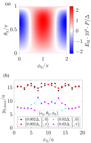
Figure 3: Majorana hybridization for a ferromagnetic chain on a 2D spin-orbit coupled superconductor (continuum model): (a) Effective Majorana hybridization $E_{\rm M}\cdot P$ as a function of the magnetic orientation of the single magnetic adatom $\theta_{\rm S}$ and $\phi_{\rm S}$ for $\epsilon_{\rm S}=0.002\Delta,\leavevmode\nobreak\ \boldsymbol{R}_{\rm S}=(8a,0.58a)$. The white region shows the crossing of the MZMs resulting in the change of the ground state parity. This result is qualitatively the same as Fig. 2(a). (b) Maximal distance $y_{\rm S,max}$ of the adatom to the $x$ axis where decoupling can be achieved in dependence on $x_{\rm S}$ for several $\phi_{\rm S}$ and $\epsilon_{\rm S}$ values and fixed $\theta_{\rm S}=\pi/2$. For both panels, $\xi_{\rm sc}=5a\Delta,\leavevmode\nobreak\ R=20a,\leavevmode\nobreak\ N_{\rm L}=N_{\rm R}=100,\epsilon_{0}=0.005\Delta$, and spin-orbit coupling strength $\lambda=0.09$.

Having demonstrated the Majorana shielding effect with continuum superconductors we next turn our attention towards lattice models for the superconducting substrate.

III.2 Lattice model for the superconducting substrate: Ferromagnetic chains on a superconductor with non-vanishing spin-orbit coupling

We next consider ferromagnetic adatom chains on a 2D superconducting square lattice with Rashba spin-orbit coupling, which has been used to describe several experimental reports of signatures of topological superconductivity in atomic chains [30, 37, 35, 56]. The lattice model incorporates the full bandwidth and the lattice symmetries of the system. The continuum models in Sec. III.1 can be obtained by expanding the lattice model around small momenta and keeping only the lowest orders.

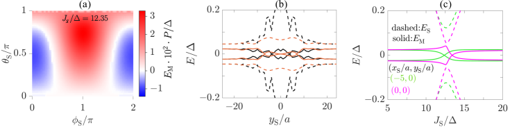
Figure 4: Majorana hybridization for ferromagnetic chains on a 2D square lattice $s$-wave superconductor with spin-orbit coupling. (a) Effective Majorana hybridization $E_{\rm M}\cdot P$ as a function of $\phi_{\rm S}$ and $\theta_{\rm S}$ for a single magnetic adatom placed at $(x_{\rm S}/a,y_{\rm S}/a)=(-5,0)$. The behavior is qualitatively similar to continuum superconductors shown in Figs. 2(a) and Fig. 3(a). (b) Effective YSR and Majorana hybridization $E$ vs. $y$ for a single magnetic adatom with fixed $x_{\rm S}/a=-5$ (black) and $x_{\rm S}/a=5$ (brown) for $\left(\phi_{\rm S},\theta_{\rm S}\right)=\left(0,0\right)$. (c) $E$ vs. $J_{\rm S}$ for a magnetic adatom at different positions. The calculation is carried out on an $81\times 81$ square lattice with $\Delta=0.2t,\,\lambda=0.3t,\,\mu=0.5t,\,t=1$ and $R/a=21$. The chains are in the topologically nontrivial phase with $J/\Delta=11.2$, resulting in $\epsilon_{\rm M}/\Delta=0.035,\,\Delta_{\rm t}/\Delta\approx 0.4$.

In order to a priori exclude the outer MZMs, $\gamma_{L}^{\prime}$ and $\gamma_{R}^{\prime}$, depicted in Fig. 1(a), we consider a slightly altered setup, where the outer ends of the chains are connected by periodic boundary conditions. We similarly use periodic boundary conditions for the substrate. Thus, the components of the Hamiltonian are [90, 91, 92, 93]

$$\begin{split}&H=H_{\rm SC}+H_{\rm R+L}+H_{\rm S}\text{, where}\\ &H_{\rm SC}=\sum_{\mathbf{m},\mathbf{b},\alpha}\left[\left(4t-\mu\right)c^{\dagger}_{\mathbf{m},\alpha}c_{\mathbf{m},\alpha}-tc^{\dagger}_{\mathbf{m}+\mathbf{b},\alpha}c_{\mathbf{m},\alpha}\right]\\ &+\sum_{\mathbf{m},\mathbf{b}}\left[-\lambda e^{i\theta_{\mathbf{b}}}c_{\mathbf{m}+\mathbf{b},\downarrow}^{\dagger}c_{\mathbf{m},\uparrow}+\Delta c^{\dagger}_{\mathbf{m},\uparrow}c^{\dagger}_{\mathbf{m},\downarrow}+\mathrm{h.c.}\right],\\ &H_{\rm R+L}=JS\sum_{m_{y}}\sum_{m_{x}=1}^{N_{\rm L}+N_{\rm R}}\sum_{\alpha,\beta}\sigma_{\alpha\beta}^{z}c_{\mathbf{m},\alpha}^{\dagger}c_{\mathbf{m},\beta}\,\delta_{m_{y},\frac{M_{y}+1}{2}},\\ &H_{\rm S}=J_{\rm S}\sum_{\alpha,\beta}(\boldsymbol{\sigma}\cdot\boldsymbol{S}_{\rm S})_{\alpha\beta}c_{N_{\rm L}+R_{\rm S},\alpha}^{\dagger}c_{N_{\rm L}+R_{\rm S},\beta}.\end{split}$$ (9)

Here, $H_{\rm R+L}$ is the Hamiltonian of the left and the right chains, connected by the periodic boundary condition. The operator $c^{\dagger}_{m,\alpha}$ creates an electron with spin $\alpha$ at site $\mathbf{m}=\left(m_{x},m_{y}\right)$ on the $M_{x}\times M_{y}$ 2D lattice, while $\sigma^{\nu}$ are the Pauli matrices in spin space. In $H_{\rm SC}$, $t$ is the nearest neighbor hopping strength, $\mu$ is the homogeneous chemical potential, and $\lambda$ is the strength of the Rashba spin-orbit coupling, which has directional dependencies given by the polar coordinates $\theta_{\mathbf{b}}$ of the nearest-neighbor bond vectors $\mathbf{b}$. This Hamiltonian, in addition to breaking time-reversal symmetry through $H_{\rm R+L}$ and $H_{\rm S}$, also breaks the spin rotation symmetry through spin-orbit coupling. Thus, this system also belongs to class D in the Cartan-Altland-Zirnbauer classification scheme for topological superconductors [79, 80].

We proceed numerically by diagonalizing the Hamiltonian within the Bogoliubov-de-Gennes formalism and extract the low-energy levels and their corresponding eigenvectors using the iterative Lanczos method, which is applicable because of the sparse Bogoliubov-de-Gennes Hamiltonian, enabling us to handle lattices corresponding to $\sim 10^{4}\times 10^{4}$ matrices for studying the low-energy physics [94, 95]. We find qualitatively similar results as for the continuum superconductors in Sec. III.1, underlining the model independence of our results. In particular, the Majorana hybridization as a function of the spin orientation of the single magnetic adatom shows a clear shielding effect with concomitant changes in the parity of the ground state, see Fig. 4(a).

In Sec. III.1.2, we defined the $y$ offset of the magnetic adatom $y_{\rm S}<y_{\rm S,max}$ to obtain Majorana shielding, see Fig. 3(b). For the lattice model here, we find $y_{\rm S,max}$ to be a few lattice sites away from the chains. Figure 4(b) is a representative plot of the in-gap levels $E_{\rm M}$ and $E_{\rm S}$ as functions of $y_{\rm S}$ for different $x_{\rm S}$. The exchange coupling, $J_{\rm S}$, between the single magnetic adatom and the superconductor, also tunes the Majorana hybridization, as shown in Fig. 4(c) for two positions of the single magnetic adatom. This is expected since $J_{\rm S}$ determines $\epsilon_{\rm S}$, corroborating the dependence of the ingap states on the bare YSR energy and its control of the shielding effect shown in Fig. 2(c). It is worth mentioning that at small and large $J_{\rm S}$, the bare YSR energy, $\epsilon_{\rm S}$, exceeds the topological gap and thus the effective MZM-YSR coupling is almost vanishing, i.e., $E_{\rm M}\approx\epsilon_{\rm M}$, in that regime.

IV Experimental considerations

In this section, we discuss possible experimental approaches for manipulating and detecting the described Majorana hybridization. A priori, there are several parameters that can be tuned to control the hybridization: the single adatom’s position on the substrate, the induced YSR energy, and the orientation of the adatom spin. The inter-chain distance $R$ is difficult to alter, thus we consider it fixed in our analysis. One of the caveats of the YSR route for designing unconventional superconducting devices is that the magnetic adatoms can be changed on the time scale of milliseconds to seconds, making it impossible to alter this system parameter within the coherence time of the MZM. One way to circumvent such parameter rigidity is to trigger the magnetic adatom spin dynamics in ESR-STM setups, a technique that has gained a lot of attention due to its sub-$\mu$eV energy resolution and its ability to detect and manipulate the spin of single atoms  [72, 73, 96, 75]. An applied radio-frequency voltage between an STM tip, harboring a spin ${\boldsymbol{S}}_{\rm tip}$, and the substrate induces a variation in the tip-substrate distance, which in turn creates a modulation of the exchange coupling $J_{\rm ex}$ between ${\boldsymbol{S}}_{\rm tip}$ and the spin ${\boldsymbol{S}}_{\rm S}$ of the single magnetic adatom, which effectively generates an $ac$ magnetic field that can drive the latter. While a full description of the adatom spin dynamics is beyond the scope of the paper, here we provide a short account of the effective model that has been used to describe ESR-STM measurements. A minimal adatom spin Hamiltonian consistent with the experimental findings reads [97, 98]:

$$\mathcal{H}_{m}(t) =-KS_{{\rm S},z}^{2}+\gamma{\boldsymbol{B}}(t)\cdot{\boldsymbol{S}}_{\rm S}\,,$$ (10)

where $K>0$ is the easy-axis anisotropy, $\gamma$ is the gyromagnetic factor, and ${\boldsymbol{B}}(t)=(J_{\rm ex}(t)/\gamma)\langle{\boldsymbol{S}}_{\rm tip}\rangle+{\boldsymbol{B}}_{\rm ex}$ is the total magnetic field acting on the adatom, being the sum of the time-dependent exchange bias and the externally applied field. Here, $\langle{\boldsymbol{S}}_{\rm tip}\rangle$ is the average spin of the tip which is determined by both the external magnetic field ${\boldsymbol{B}}_{\rm ex}$, and local anisotropies [74]. The equilibrium orientation of the adatom spin, ${\boldsymbol{S}}_{\rm S}(\theta_{\rm S},\phi_{\rm S})$, can be found by minimizing the energy in Eq. (10). Since $J_{\rm ex}\propto\exp(-d/d_{\rm ex})$ [74], with $d_{\rm ex}$ a characteristic length, changing the tip height $d$ could facilitate the rotation of the spin ${\boldsymbol{S}}_{\rm S}$ by arbitrary angles $\{\theta_{\rm S},\phi_{\rm S}\}$. We note in passing that the term $\sim S_{{\rm S},z}^{2}$ is generated by the breaking of the inversion symmetry of the surface states and, on a more fundamental level, enables the use of the classical approximation for describing the adatom spin [99, 100].

The same Hamiltonian in Eq. (10) can be harnessed for the readout of the electronic state in ESR-STM measurements. To demonstrate that, we first stress that the electronic spin density at the position of the adatom ${\boldsymbol{R}}_{S}$ can act back on the spin ${\boldsymbol{S}}_{\rm S}$ via their exchange coupling $J$, or the effective magnetic field ${\boldsymbol{B}}_{n}=(J/\gamma)\langle{\boldsymbol{\sigma}}({\boldsymbol{R}}_{\rm S})\rangle_{n}$, where $\langle{\boldsymbol{\sigma}}({\boldsymbol{R}}_{\rm S})\rangle_{n}\equiv\langle\psi_{n}|{\boldsymbol{\sigma}}({\boldsymbol{R}}_{\rm S})|\psi_{n}\rangle$ represents the superconductor condensate’s spin expectation value at the position of the adatom in the many-body state $|\psi_{n}\rangle$. Consequently, the dynamics of the adatom spin depends on the electronic state via the total magnetic field

$${\boldsymbol{B}}_{n,\rm tot}={\boldsymbol{B}}+{\boldsymbol{B}}_{n}\,,$$ (11)

which in turn influences ${\boldsymbol{S}}_{\rm S}\equiv{\boldsymbol{S}}_{{\rm S},n}$ and hence the resonance condition. The jiggling of the STM tip height $d$ at a frequency $\omega$ would give rise to a time-dependent magnetic field $\boldsymbol{B}_{\rm ac}(t)\perp{\boldsymbol{S}}_{{\rm S},n}\propto\delta J_{\rm ex}\cos(\omega t)$, with $\delta J_{\rm ex}$ the amplitude of the $ac$ field. Then, sweeping $\omega$ should allow for extracting the electronic state-dependent resonance frequency in ESR-STM measurements [73, 101, 102].

Another viable way to accomplish full control of the hybridization is to place a single magnetic adatom directly on a superconducting STM tip, instead of the bulk superconductor. Its interaction with the bulk superconductor (and hence its YSR energy) can be tuned by changing the STM tip height, while its placement on top of the superconductor can be arbitrary  [103, 75, 104, 105]. The ESR-STM technique would work analogously to the intrinsic adatom case described above, albeit the microscopic coupling parameters and their scaling with the STM position would need a separate investigation.

The detection of the ESR signal is performed in conductance measurements, and thus the effective $ac$ fields that drive the impurity pertain to charge currents flowing into the YSR state, causing relaxation and dephasing via inelastic electron tunneling. Hence, both the manipulation and detection need to be performed on time scales shorter than the induced decoherence time $T_{2}$. Time scales on the order of $T_{2}\sim 10^{2}\mu$s have been reported recently for adatoms on normal metals [73], making such technique particularly attractive also for superconducting substrates.

V Concluding remarks

In this work, we have demonstrated efficient control of the hybridization of Majorana zero modes in magnetic chains-superconductor systems by using an additional magnetic adatom in the proximity of the chain. We found that the adatom parameters, such as the spin orientation, the exchange coupling to the superconductor, and its position on the substrate can all alter the Majorana spectrum. Specifically, we have shown that the Majorana shielding, i.e., the complete suppression of the Majorana hybridization, and ground state parity flipping are not only possible but are universal and model-independent. Experimentally, the manipulation of the single magnetic adatom parameters and hence the MZMs hybridization could be implemented by using the mature STM and ESR-STM techniques. Our study, therefore, opens a potential route toward experiments that directly probe the non-Abelian character of MZMs in magnetic chain-superconductor platforms. Moreover, it could facilitate the implementation of a universal set of quantum gates with Majorana qubits. Furthermore, successful control of Majorana hybridization is an essential prerequisite for fusion and several braiding schemes of MZMs [106, 77, 68]. To this end, we envision networks of chain-adatom-chain constructions that allow for the time-dependent tuning of multiple MZM hybridizations at junctions with additional single magnetic adatoms.

In the remainder of the discussion, we emphasize two potential applications of our results beyond the aforementioned ones. Recently, STM experiments have constructed magnetic adatom chains on a superconductor atom by atom and have probed the chains at both ends. However, the chains achieved so far are not long enough, leading to strongly hybridized MZMs, termed precursors of Majorana modes, whose hybridization energy oscillates with chain length [56]. Our proposal shows a path to alleviate this problem. By relaxing the condition that the MZMs on the same chain do not couple and focusing on a single chain, our proposal reduces to the short chain-superconductor system with precursors of Majorana modes, which can be tuned to zero energy by placing a single magnetic adatom close to one end of the chain, following the procedures of our proposal. We have checked numerically that the tunability of the precursors’ energy is qualitatively the same as for the MZMs in long double chains in Sec. III. Thus, our proposal can be tested immediately at the level of current experiments in existing devices. The most direct test would be to position an additional magnetic adatom at various positions close to a chain that accommodates precursors of Majorana modes with finite energy and determine the ideal position for Majorana shielding by minimizing the observed energy of the precursors the STM spectrum.

Another exciting future direction concerns the quantum nature of the adatoms spin and its effects on the Majorana hybridization. Indeed, while here we have used a classical description of the spins which is valid in the limit of large spins and/or large easy axis anisotropies, recent works suggest that quantum effects can become important for smaller spins [107, 108]. In particular, the Kondo-like screening of the adatoms’ spins by the Shiba electrons could have dramatic consequences on the Majorana hybridization, and on the topological phase diagram in general in our model. Hence, it would be interesting to explore the resulting dynamics pertaining to the coupling between the two quantum systems and eventually establish efficient ways to control the Majorana hybridization in ESR-STM experiments [100].

Appendix A Local density of states of the effective low-energy model model

In Sec. II of the main text, we mention the dependence of the localization of the low-energy states on the parameters of the single magnetic adatom. Here, we present a general analytical derivation of the Majorana weight, $W_{\rm M}$, which is the local density of states of the MZMs at the position of the single magnetic adatom, $d$. We obtain the Green’s function of the effective low-energy Hamiltonian, Eq. (1) in the main text, by solving the Green’s functions equations of motion in the basis $\left(f,d,f^{\dagger},d^{\dagger}\right)$ given above Eq. (2) in the main text. The electronic component of the single magnetic adatom’s Green’s function is

$$G_{dd^{\dagger}}(E)=\dfrac{A(E)}{(E^{2}-E_{S}^{2})(E^{2}-E_{M}^{2})},$$ (12)

where we have defined

$$A(E)=(E^{2}-\epsilon_{\rm M}^{2})(E+\epsilon_{\rm S})-(E-\epsilon_{\rm M})|t_{1}|^{2}-(E+\epsilon_{\rm M})|t_{2}|^{2}.$$ (13)

As a consistency check, we observe that the poles of the Green’s function appear at the effective energies of Eq. (2). This yields the local density of states as LDOS($E$)= $-\lim_{n\to 0}\Im{G_{dd^{\dagger}}(E+in)}/\pi.$ We find

$${\rm LDOS}(E)=\dfrac{A(E_{M})\delta(E-E_{M})+A(-E_{M})\delta(E+E_{M})-A(E_{S})\delta(E-E_{S})-A(-E_{S})\delta(E+E_{S})}{2E(E_{M}^{2}-E_{S}^{2})},$$ (14)

which, integrated over energy, equals one, as it should for a single particle state. Hence, the Majorana weight at the single magnetic adatom becomes

$$W_{\rm M}=\dfrac{A(E_{M})-A(-E_{M})}{2(E_{M}^{2}-E_{S}^{2})E_{M}}=\dfrac{E_{M}^{2}-\epsilon_{\rm M}^{2}-|t_{1}|^{2}-|t_{2}|^{2}}{E_{M}^{2}-E_{S}^{2}}.$$ (15)

We can rewrite Eq. (15) as

$$W_{\rm M}=\dfrac{1}{2}-\dfrac{\epsilon_{S}^{2}-\epsilon_{M}^{2}}{2\sqrt{\left((\epsilon_{S}-\epsilon_{M})^{2}+4\mid t_{\rm L}-it_{\rm R}\mid^{2}\right)\left((\epsilon_{S}+\epsilon_{M})^{2}+4\mid t_{\rm L}+it_{\rm R}\mid^{2}\right)}}.$$ (16)

From the above, we check three different limits. First, if $\epsilon_{\rm S}=\epsilon_{\rm M}$ and $|t_{\rm L}|\neq 0$ or $|t_{\rm R}|\neq 0$, the Majorana LDOS at the position of the single YSR adatom is exactly $\dfrac{1}{2}$. Next, in the large hybridization limit, i.e, $|t_{1}|,|t_{2}|\gg\epsilon_{\rm S},\epsilon_{\rm M}$ the Majorana LDOS is again $\dfrac{1}{2}$. On the other hand, in the small hybridization limit, i.e, $\epsilon_{\rm S},\epsilon_{\rm M}\gg|t_{1}|,|t_{2}|$ the Majorana LDOS at the single adatom vanishes. In order to determine the spatial distribution of the MZM at the parameters of Majorana shielding, we calculate the Majorana LDOS at $E_{\rm M}=0$

$$W_{\rm M,0}=\dfrac{1}{2}-\dfrac{1}{2}\dfrac{\epsilon_{\rm S}^{2}-\epsilon_{\rm M}^{2}}{\left(\epsilon_{\rm S}-\epsilon_{\rm M}\right)^{2}+4\mid t_{\rm 1,0}\mid^{2}}=\dfrac{1}{2}-\dfrac{1}{2}\dfrac{\epsilon_{\rm S}^{2}-\epsilon_{\rm M}^{2}}{\epsilon_{\rm S}^{2}+\epsilon_{\rm M}^{2}+4\mid t_{\rm L,0}\mid^{2}+4\mid t_{\rm R,0}\mid^{2}}=\dfrac{1}{2}-\dfrac{1}{2}\dfrac{\epsilon_{\rm S}^{2}-\epsilon_{\rm M}^{2}}{E_{\rm S,0}^{2}},$$ (17)

where $E_{\rm S,0}$ is the YSR effective energy and $t_{1,0}$ the hopping parameter at the Majorana shielding points. The parameters $t_{L,0}$ and $t_{R,0}$ generally depend on $\epsilon_{\rm S}$ and $\epsilon_{\rm M}$ themselves. On the other hand, $W_{\rm M,0}$ cannot be expressed solely in terms of $\epsilon_{\rm S}$ and $\epsilon_{\rm M}$. If $|\epsilon_{\rm S}|\gg|\epsilon_{\rm M}|$, the Majorana shielding is complete $W_{\rm M,0}\approx 0$. On the other hand, when $1\gg\epsilon_{\rm S}-\epsilon_{\rm M}>0$, the Majorana LDOS at the position of the single magnetic adatom is maximal and the states are completely mixed $W_{\rm M,0}\approx\dfrac{1}{2}$.

Appendix B Parity change at zero energy crossing

We mentioned in the main text that the fermion parity of the ground state changes only through a zero-energy level crossing in symmetry class $D$. Due to the small size of the Hamiltonian in Eq. (1), we can demonstrate this behavior explicitly and give details on the polarization of the states. To this end, we investigate the changes in the ground state parity as the parameters of the single magnetic adatom are tuned. We consider the effective low-energy Hamiltonian, Eq. (1), in Fock space in the basis $|n_{f},n_{d}\rangle=\left(f^{\dagger}\right)^{n_{f}}\left(d^{\dagger}\right)^{n_{d}}|00\rangle$, where $n_{f/d}=0,1$ is the fermion occupation of the non-local fermion/YSR state, and the parity of the states is defined as $P=\left(-1\right)^{n_{f}+n_{d}}$. The many-body energies in the odd/even subspaces $E_{\pm}^{\rm o/e}$ are obtained as,

$$\begin{split}E_{\pm}^{\rm e}&=\frac{1}{2}\left[\epsilon_{+}\pm\sqrt{\epsilon_{+}^{2}+4|t_{-}|^{2}}\right],\\ E_{\pm}^{\rm o}&=\frac{1}{2}\left[\epsilon_{+}\pm\sqrt{\epsilon_{-}^{2}+4|t_{+}|^{2}}\right],\end{split}$$ (18)

and their corresponding eigenstates are $|V_{\pm}^{\rm e}\rangle=\pm v_{00}|00\rangle+v_{11}|11\rangle$ and $|V_{\pm}^{\rm o}\rangle=\pm v_{10}|10\rangle+v_{01}|01\rangle$ are linear combinations of $|n_{f},n_{d}\rangle$, with amplitudes $v_{n_{f}n_{d}}$, within a single fermion parity sector.

We see that $E_{-}^{\rm o}$ and $E_{-}^{\rm e}$ are the lower energies and either of them can be the ground state energy, while $E_{+}^{\rm o}$ and $E_{+}^{\rm e}$ are higher in energy. Even and odd states cross at the degenerate point $E_{-}^{\rm o}=E_{-}^{\rm e}$ $\left({\rm}\leavevmode\nobreak\ E_{+}^{\rm o}=E_{+}^{\rm e}\right)$ accompanied by a fermion parity switching. From Eq. (18), we see that the condition for the many-body ground state degeneracy is the same as the Majorana shielding condition of Eq. (3).

Appendix C Derivation of generalized low-energy model coupling, $t_{\rm L/R}$

In Eq. (6) in Sec. III.1 of the main text, we presented the generalized expression of the coupling between YSR state and the MZMs in the left and right chains, $t_{\rm L/R}$. Here, we give a detailed derivation of these quantities, independently of the microscopic model. We first consider the Hamiltonian that describes the coupling of the left chain to the single magnetic adatom, obtained from the last line of Eq. (4) in the main text, as

$$H_{\rm LS}=d^{\dagger}\sum_{m}h_{N_{L}+\frac{R_{S}}{a},m}b_{Lm}+\Delta_{N_{L}+\frac{R_{S}}{a},m}b_{Lm}^{\dagger}+d\sum_{m}-h_{N_{L}+\frac{R_{S}}{a},m}b^{\dagger}_{Lm}+\Delta_{N_{L}+\frac{R_{S}}{a},m}b_{Lm}.$$ (19)

We make a basis transformation of Eq. (19)

$$H_{\rm LS}=d^{\dagger}\left(t_{\rm L}\gamma_{L}+\sum_{m}q_{m}p_{m}\right)+\left(t^{*}_{L}\gamma_{L}+\sum_{m}q^{*}_{m}p_{m}^{\dagger}\right)d,$$ (20)

where $\gamma_{\rm L},p_{i}$ correspond to the Majorana operator and the YSR band orbitals of the left chain, respectively, and $q_{i}$ are unknown matrix elements. Next, we extract the matrix element $t_{\rm L}$ via

$$t_{\rm L}=\dfrac{1}{2}\{d,[H_{\rm LS},\gamma_{\rm L}]\}.$$ (21)

By expressing the Majorana solution in the fermionic basis in the second quantized formalism, Eq. (21) yields

$$t_{\rm L}=\sum_{m}\left[u_{m}h_{N_{L}+\frac{R_{S}}{a},m}+v_{m}\Delta_{N_{L}+\frac{R_{S}}{a},m}\right],$$ (22)

where $u_{m}$ and $v_{m}$ are the particle and hole components of the Majorana solutions’ BdG eigenmode. We evaluate the matrix elements $h_{N_{L}+\frac{R_{S}}{a},m}$ and $\Delta_{N_{L}+\frac{R_{S}}{a},m}$ of Eq. (5) from the following equations,

$$\begin{split}\langle\uparrow(N_{L}+\frac{R_{S}}{a})\mid\uparrow\left(m\right)\rangle=&\cos(\theta_{\rm S}/2)e^{i\phi_{\rm S}/2}\cos(\theta_{m}/2)e^{-i\phi_{\rm m}/2}+\sin(\theta_{\rm S}/2)e^{-i\phi_{\rm S}/2}\sin(\theta_{m}/2)e^{i\phi_{m}/2},\\ \langle\uparrow(N_{L}+\frac{R_{S}}{a})\mid\downarrow\left(m\right)\rangle=&\cos(\theta_{\rm S}/2)e^{i\phi_{\rm S}/2}\sin(\theta_{m}/2)e^{-i\phi_{m}/2}-\sin(\theta_{\rm S}/2)e^{-i\phi_{\rm S}/2}\cos(\theta_{m}/2)e^{i\phi_{m}/2},\\ \langle\uparrow(N_{L}+\frac{R_{S}}{a})\mid i\sigma_{y}\mid\uparrow\left(m\right)\rangle=&\cos(\theta_{\rm S}/2)e^{i\phi_{\rm S}/2}\sin(\theta_{m}/2)e^{i\phi_{m}/2}-\sin(\theta_{\rm S}/2)e^{-i\phi_{\rm S}/2}\cos(\theta_{m}/2)e^{-i\phi_{m}/2},\\ \langle\uparrow(N_{L}+\frac{R_{S}}{a})\mid i\sigma_{y}\mid\downarrow\left(m\right)\rangle=&-\cos(\theta_{\rm S}/2)e^{i\phi_{\rm S}/2}\cos(\theta_{m}/2)e^{i\phi_{m}/2}-\sin(\theta_{\rm S}/2)e^{-i\phi_{\rm S}/2}\sin(\theta_{m}/2)e^{-i\phi_{m}/2}.\end{split}$$ (23)

By substituting the matrix elements in Eq. (22), the general form of $t_{\rm L}$ is expressed as

$$t_{\rm L}=e^{i\frac{\phi_{\rm S}}{2}}\cos\left(\frac{\theta_{\rm S}}{2}\right)\,F_{L}+e^{-i\frac{\phi_{\rm S}}{2}}\sin\left(\frac{\theta_{\rm S}}{2}\right)\,G_{\rm L},$$ (24)

which is presented in Eq. (6) in Sec. III.1 of the main text. Here,

$$\begin{split}F_{\rm L}=&\dfrac{1}{2}\sum_{m=0}^{\infty}u_{m}\left(h^{(0)}_{N_{L}+\frac{R_{S}}{a},m}\cos(\theta_{m}/2)e^{-i\phi_{\rm m}/2}+h^{(1)}_{N_{L}+\frac{R_{S}}{a},m}\sin(\theta_{m}/2)e^{i\phi_{\rm m}/2}\right)\\ &+v_{m}\left(\Delta^{(0)}_{N_{L}+\frac{R_{S}}{a},m}\sin(\theta_{m}/2)e^{-i\phi_{\rm m}/2}-\Delta^{(1)}_{N_{L}+\frac{R_{S}}{a},m}cos(\theta_{m}/2)e^{i\phi_{\rm m}/2}\right),\\ G_{\rm L}=&\dfrac{1}{2}\sum_{m=0}^{\infty}u_{m}\left(h^{(0)}_{N_{L}+\frac{R_{S}}{a},m}\sin(\theta_{m}/2)e^{i\phi_{\rm m}/2}-h^{(1)}_{N_{L}+\frac{R_{S}}{a},m}\cos(\theta_{m}/2)e^{-i\phi_{\rm m}/2}\right)\\ &-v_{m}\left(\Delta^{(0)}_{N_{L}+\frac{R_{S}}{a},m}\cos(\theta_{m}/2)e^{i\phi_{\rm m}/2}+\Delta^{(1)}_{N_{L}+\frac{R_{S}}{a},m}\sin(\theta_{m}/2)e^{-i\phi_{\rm m}/2}\right).\end{split}$$ (25)

Hence, we explicitly show the dependence of the coupling of the YSR state to the MZM on the orientation of the single magnetic adatom. Notably, from Eq. (25), we establish that

$$F_{\rm L}(\phi_{m},\theta_{m})=G_{\rm L}(-\phi_{m},\pi-\theta_{m}).$$ (26)

A similar form can be derived for $t_{\rm R}$ by substituting the Majorana solution and the matrix elements of the right chain.

So far, we have derived the general expressions without the microscopic details of the chains and superconductor. We next focus on special cases which are model dependent.

C.1 Special Case: Helical Chains Model

Let us consider the special case where the spins of magnetic adatoms in the chains form a planar helix with $\theta_{m}=\theta=\pi/2$ and a chiral symmetry $\mathcal{C}$ is present in the system.This specific case corresponds to the model presented in Sec. III.1.1. For $\mathcal{C}=\sigma_{y}$, the zero energy modes of the chains will be chiral counterparts of the $\mathcal{C}$ operator. Here, $\sigma_{y}$ is a Pauli matrix which acts on the basis of the particle-hole components of the YSR orbitals. This constraints the form of the BdG eigenspinors of the Majoranas to satisfy $v_{m}=iu_{m}$ for the $\gamma_{\rm L}$ [29]. The equality $u^{*}=v$ holds due to particle-hole symmetry. Under these assumptions, we compute

$$F_{\rm L}^{*}=\dfrac{1}{2\sqrt{2}}\sum_{m}e^{i\phi_{\rm m}/2}\left(v_{m}h^{(0)}_{N_{L}+\frac{R_{S}}{a},m}+u_{m}\Delta^{(0)}_{N_{L}+\frac{R_{S}}{a},m}\right)=\dfrac{i}{2\sqrt{2}}\sum_{m}u_{m}e^{i\phi_{\rm m}/2}\left(h^{(0)}_{N_{L}+\frac{R_{S}}{a},m}-i\Delta^{(0)}_{N_{L}+\frac{R_{S}}{a},m}\right)=iG_{\rm L}.$$ (27)

We conclude that $G_{\rm L}=-iF^{*}_{\rm L}$ as mentioned in Sec. III.1.1 of the main text. It follows that $G^{*}_{\rm L}=iF_{\rm L}$ and $|G_{\rm L}|=|F_{\rm L}|$. Similarly, we obtain $F^{*}_{\rm R}=-iG_{\rm R}$. Using the above, we calculate the absolute value of the coupling $|t_{\rm L}|^{2}$ from Eq. (24). We arrive at

$$|t_{\rm L}|^{2}=|G_{\rm L}|^{2}+2\sin\left(\dfrac{\theta_{d}}{2}\right)\cos\left(\dfrac{\theta_{d}}{2}\right)\Re\left[ie^{i\phi_{\rm S}}G^{2}_{L}\right].$$ (28)

Here $|t_{\rm L}|^{2}$ is symmetric for $\theta_{S}\rightarrow\pi-\theta_{S}$, as expected. This derivation is general in the sense that we have not assumed a semi-infinite chain and do not restrict our calculations to the Bragg point $k_{F}=k_{h}$.

C.2 Special case: Ferromagnetic Chains Model

We now consider the model presented in Sec. III.1.2. In the case where the magnetizations of the YSR atoms of the chains are pointing perpendicular to the SOC plane of the substrate in the z direction, the effective BdG Hamiltonians of each of the chains acquire an extra chiral symmetry $\mathcal{\tilde{C}}=\sigma_{x}$. This implies that the Majorana BdG eigenspinors are restricted to be eigenstates of $\sigma_{x}$. This implies $u_{\rm L}=-v_{\rm L}$ and $u_{\rm R}=v_{\rm R}$ or $u_{\rm R}=-v_{\rm R}$ and $u_{\rm L}=v_{\rm L}$. Without loss of generality, we focus on the first case. Combining that with the reality condition of the Majorana wavefunction, we conclude that $u_{\rm R}=v_{\rm R}=u$ and $u_{\rm L}=-v_{\rm L}=iu$, where $u$ is real. We verified the above by a numerical evaluation of the Majorana wavefunctions. In that case, the parameters in Eq. (25) can be simplified to

$$\begin{split}F_{\rm L}=&\dfrac{1}{2}\sum_{m=0}^{\infty}u_{Lm}h^{(0)}_{N_{L}+\frac{R_{S}}{a},m}-v_{Lm}\Delta^{(1)}_{N_{L}+\frac{R_{S}}{a},m}=\dfrac{i}{2}\sum_{m=0}^{\infty}u_{m}\left(h^{(0)}_{N_{L}+\frac{R_{S}}{a},m}+\Delta^{(1)}_{N_{L}+\frac{R_{S}}{a},m}\right),\\ G_{\rm L}=&-\dfrac{1}{2}\sum_{m=0}^{\infty}u_{Lm}h^{(1)}_{N_{L}+\frac{R_{S}}{a},m}+v_{Lm}\Delta^{(0)}_{N_{L}+\frac{R_{S}}{a},m}=-\dfrac{i}{2}\sum_{m=0}^{\infty}u_{m}\left(h^{(1)}_{N_{L}+\frac{R_{S}}{a},m}-\Delta^{(0)}_{N_{L}+\frac{R_{S}}{a},m}\right),\end{split}$$ (29)

where the matrix elements$h^{0(1)},\Delta^{0(1)}$ are calculated in Appendix F. We write the same expressions for $t_{\rm R}$

$$\begin{split}F_{\rm R}=&\dfrac{1}{2}\sum_{m=0}^{\infty}u_{Rm}\tilde{h}^{(0)}_{N_{L}+\frac{R_{S}}{a},m}-v_{Rm}\tilde{\Delta}^{(1)}_{N_{L}+\frac{R_{S}}{a},m}=\dfrac{1}{2}\sum_{j=0}^{\infty}u_{m}\left(\tilde{h}^{(0)}_{N_{L}+\frac{R_{S}}{a},m}-\tilde{\Delta}^{(1)}_{N_{L}+\frac{R_{S}}{a},m}\right),\\ G_{\rm R}=&-\dfrac{1}{2}\sum_{m=0}^{\infty}u_{Rm}\tilde{h}^{(1)}_{N_{L}+\frac{R_{S}}{a},m}+v_{Rm}\tilde{\Delta}^{(0)}_{N_{L}+\frac{R_{S}}{a},m}=-\dfrac{1}{2}\sum_{m=0}^{\infty}u_{m}\left(\tilde{h}^{(1)}_{N_{L}+\frac{R_{S}}{a},m}+\tilde{\Delta}^{(0)}_{N_{L}+\frac{R_{S}}{a},m}\right),\end{split}$$ (30)

where the tilded matrix elements couple the single magnetic adatom to the right chain and the index j runs over the right chain. We now focus on the case where the single magnetic adatom is placed exactly in the middle of the two chains $R_{\rm S}=R/2$. Notably, the elements $h^{1(0)}$ and $\Delta^{1(0)}$ are odd( even) functions of the relative positions of the YSR states. We rewrite the matrix elements Eq. (30)

$$\begin{split}F_{\rm R}=&\dfrac{1}{2}\sum_{m=0}^{\infty}u_{m}\left(h^{(0)}_{N_{L}+\frac{R_{S}}{a},m}+\Delta^{(1)}_{N_{L}+\frac{R_{S}}{a},m}\right),\\ G_{\rm R}=&=-\dfrac{1}{2}\sum_{m=0}^{\infty}u_{m}\left(-h^{(1)}_{N_{L}+\frac{R_{S}}{a},m}+\Delta^{(0)}_{N_{L}+\frac{R_{S}}{a},m}\right).\end{split}$$ (31)

We establish that $F_{\rm L}-iF_{\rm R}=0$ and also $G_{\rm L}+iG_{\rm R}=0$. From Eq. (2), it is evident that $\phi_{\rm S}$ enters $E_{\rm M}$ in the terms $t^{2}_{\pm}=|t_{\rm L}\mp it_{\rm R}|^{2}$. Thus, we compute

$$|t_{\rm L}+it_{\rm R}|= |e^{i\phi_{\rm S}}\cos\left(\dfrac{\theta_{S}}{2}\right)\left(F_{\rm L}+iF_{\rm R}\right)|=|\cos\left(\dfrac{\theta_{S}}{2}\right)\left(F_{\rm L}+iF_{\rm R}\right)|,$$ (32)

$$|t_{\rm L}-it_{\rm R}|= |e^{-i\phi_{\rm S}}\sin\left(\dfrac{\theta_{S}}{2}\right)\left(G_{\rm L}-iG_{\rm R}\right)|=|\sin\left(\dfrac{\theta_{S}}{2}\right)\left(G_{\rm L}-iG_{\rm R}\right)|.$$ (33)

Both the above expressions are independent of $\phi_{\rm S}$. Thus, we proved that when the single magnetic adatom is placed at the middle of the chains, its’ azimuthial orientation does not influence the hybridization of the MZMs.

Appendix D Derivation of the effective model parameters for III.1.1

In this Section, we present a detailed derivation of the low-energy parameters, $\epsilon_{\rm M},\,t_{\rm L}$ and $t_{\rm R}$, in Sec. III.1.1 of the main text. In the following, the semi-infinite chain limit and the Bragg point approximation are considered. Following [29], we rotate in the fermionic basis and express the normalized Majorana operators at the right edge of the left chain $\gamma_{\rm L}$ and at the left edge of the right chain $\gamma_{\rm R}$ as

$$\gamma_{\rm L}= \sqrt{1-\beta^{2}}\sum_{m=0}^{\infty}e^{-ln(|\beta|)m}\left(e^{i\pi/4}b_{Lm}+e^{-i\pi/4}b^{\dagger}_{Lm}\right),$$ (34)

$$\gamma_{\rm R}= \sqrt{1-\beta^{2}}\sum_{m=0}^{\infty}e^{-ln(|\beta|)m}\left(e^{-i\pi/4}b_{Rm}+e^{i\pi/4}b^{\dagger}_{Rm}\right),$$ (35)

written in the basis of the YSR creation and annihilation operators of the left and right chain, respectively, and $\beta$ is defined in the main text in Eq. (7). We note the usual exponential decay of the Majorana operators.

D.1 YSR-Majorana couplings, $t_{\rm L},\,t_{\rm R}$

Following [28], we acquire

$$h_{N_{L}+\frac{R_{S}}{a},m}= -\dfrac{\Delta}{\sqrt{2}}\dfrac{\sin(k_{F}(R_{\rm S}+am))}{k_{F}(R_{\rm S}+am)}e^{-(R_{\rm S}+am)/\xi_{\rm sc}}\left(\cos\left(\dfrac{\theta_{\rm S}}{2}\right)e^{i(\phi_{\rm S}+2k_{h}am)/2}+\sin\left(\dfrac{\theta_{\rm S}}{2}\right)e^{-i(\phi_{\rm S}+2k_{h}am)/2}\right),$$ (36)

$$\Delta_{N_{L}+\frac{R_{S}}{a},m}= \dfrac{\Delta}{\sqrt{2}}\dfrac{\cos(k_{F}(R_{\rm S}+am))}{k_{F}(R_{\rm S}+am)}e^{-(R_{\rm S}+am)/\xi_{\rm sc}}\left(\cos\left(\dfrac{\theta_{\rm S}}{2}\right)e^{i(\phi_{\rm S}+2k_{h}am)/2}-\sin\left(\dfrac{\theta_{\rm S}}{2}\right)e^{-i(\phi_{\rm S}+2k_{h}am)/2}\right).$$ (37)

We now substitute the Majorana solution from Eq. (34) in the general Eq. (24) to get

$$t_{\rm L}=\dfrac{e^{-i\pi/4}\sqrt{1-\beta^{2}}}{2}\sum_{m}\beta^{m}\left(h_{N_{L}+\frac{R_{S}}{a},m}+i\Delta_{N_{L}+\frac{R_{S}}{a},m}\right).$$ (38)

After substituting the matrix elements Eq. (36) and Eq. (37) and performing this infinite sum, we reach Eq. (7) of the main text. A similar calculation can be performed for $t_{\rm R}$ where the helicity changes sign $k_{h}\rightarrow{-k_{h}}$ in Eq. (36) and also the Majorana solution $\gamma_{\rm R}$ in Eq. (35) should be used.

D.2 Bare Majorana hybridization, $\epsilon_{M}$

In order to calculate the bare Majorana hybridization between the inner MZMs of the chains, we consider the effective Hamiltonian of Eq. (4)

$$H_{\rm LR}=\sum_{mn}b^{\dagger}_{Lm}\left(h_{mn}b_{Rn}+\Delta_{mn}b^{\dagger}_{Rn}\right)+\sum_{mn}b_{Lm}\left(\Delta_{mn}b_{Rn}-h_{mn}b^{\dagger}_{Rn}\right),$$ (39)

where $b_{Lm}$, $b_{Rn}$ are annihilation operators for electrons at the YSR orbitals in the left and right chains, respectively, and

$$h_{mn}= -\cos(k_{h}a(m+n))\dfrac{\Delta\sin(k_{F}(am+an+R))}{k_{F}(am+an+R))}e^{-\frac{am+an+R}{\xi_{\rm sc}}},$$ (40)

$$\Delta_{mn}= i\sin(-k_{h}a(m+n))\dfrac{\Delta\cos(k_{F}(am+an+R))}{k_{F}(am+an+R))}e^{-\frac{am+an+R}{\xi_{\rm sc}}},$$ (41)

are the matrix elements taken from [28]. We express Eq. (39) in the fermionic eigenbasis of the left and right chains

$$H_{\rm LR}=\dfrac{i}{2}\epsilon_{\rm M}\gamma_{\rm L}\gamma_{\rm R}+\sum_{mn}k_{m}\gamma_{\rm L}p_{Rm}+l_{n}\gamma_{\rm R}p_{Ln}+M_{mn}p_{Ln}p_{Rm}+H.c,$$ (42)

where $p_{Ln},p_{Rm}$ correspond to the electrons of the YSR band orbitals of the left and right chain, respectively. These are independent fermionic operators that anti-commute with each other. Also, $k_{m}$,$l_{n}$,$M_{mn}$ are material specific matrix elements. These a priori unknown matrix elements do not need to be calculated because we assume that the associated orbitals of the YSR bands are high in energy compared to the bare Majorana hybridization and hence they play no role in the subsequent calculations for the low-energy theory. It is straightforward to extract the element $i\epsilon_{M}$ from Eq. (42) as

$$i\epsilon_{\rm M}=\dfrac{1}{2}\{\gamma_{\rm R},[\gamma_{\rm L},H_{\rm LR}]\}.$$ (43)

Now, we substitute the Majorana operators from Eq. (34) and Eq. (35) and $H_{\rm LR}$ from Eq. (39) to obtain

$$i\epsilon_{\rm M}=(1-\beta^{2})\sum_{mn}e^{(m+n)ln(\beta)}\left(\Delta_{mn}+ih_{mn}\right).$$ (44)

Next, by substituting the matrix elements Eq. (40) and Eq. (41) and perform the double infinite sum, we acquire $\epsilon_{\rm M}(R)$ in Eq. (7) of the main text.

Appendix E Asymptotic limits

We further analyze the model in Sec. III.1.1 by taking the asymptotic limit for the parameters in Eq. (7). In our parameters, we take the asymptotic limit $R/a\rightarrow\infty$ and $R_{\rm S}/a\rightarrow\infty$ to get

$${}_{2}F_{1}(1,\frac{R}{a};\frac{R}{a}+1;e^{-A_{s}})\rightarrow \dfrac{1}{1-e^{-A_{s}}},$$ (45)

$${}_{2}F_{1}(2,\frac{R}{a}+1;\frac{R}{a}+2;e^{-A_{s}})\rightarrow \dfrac{1}{\left(1-e^{-A_{s}}\right)^{2}}.$$ (46)

Here, a 3D bulk superconductor has been assumed. For practical purposes, the limits in Eq. (45) and Eq. (46) give a good approximation for our considered setup in Fig. 2, where $R=20a$ and $\epsilon_{M}$ in Eq. (7) scales as

$$\epsilon_{\rm M}\sim\dfrac{e^{-R/\xi_{\rm sc}}}{k_{F}R}L(k_{F}R),$$ (47)

where $L(k_{F}R)$ is the oscillating part. In the dilute adatom limit that we are working with, we expect the bare Majorana hybridization to cross zero multiple times as we are increasing the distance between the chains due to the high frequency of the oscillations $k_{F}a\gg 1$. This shows that for big distances until $R\approx\xi_{\rm sc}$, there is a power law decay for the Majorana-Majorana hybridization. When $R\gg\xi_{\rm sc}$, the exponential decay dominates. In both cases, the oscillations part is present. For the parameters $t_{\rm L}$ and $t_{\rm R}$ that appear in Eq. (7), only the limit of Eq. (45) enters. The asymptotic limit of Eq. (8) for $R_{\rm S}\gg a$ is

$$\phi_{\rm S,L}(R_{\rm S})=-2k_{F}R_{\rm S}+2\arctan\dfrac{\sin(2k_{F}a)}{-e^{\frac{a}{\xi_{\rm sc}}-ln(\beta)}+\cos(2k_{F}a)}.$$ (48)

As we see in Eq. (48), the crossing angle $\phi_{\rm S,L}(R_{\rm S})$ scales linearly with the distance of the single magnetic adatom from the chain.

Appendix F Ferromagnetic chains on Continuum superconductor with non-vanishing spin-orbit coupling

In Sec. III.1.2 of the main text, we presented the results for a model of two ferromagnetic chains in a 2D continuum $s$-wave superconductor with finite Rashba spin-orbit coupling separated by a distance $R$ and a magnetic adatom placed in between at $R_{\rm S}$ away from the left chain. In this section, we give details of the extension of the model in Ref. [31] to our system. As discussed in Sec. III.1, in the dilute deep Shiba limit where the YSR states from individual magnetic adatoms are well within the superconducting gap close to the Fermi energy, the low energy effective Hamiltonian is described by Eq. (4). The matrix elements, $\mathcal{H_{\rm L}},\leavevmode\nobreak\ \mathcal{H_{\rm R}}$ and $\mathcal{H_{\rm LR}}$, for this model can be explicitly written down using Eq. (5) as

$$h_{mn}=h^{(0)}_{mn}=\frac{I^{+}_{1}(r_{mn})+I^{-}_{1}(r_{mn})}{2},\leavevmode\nobreak\ \Delta_{mn}=\Delta^{(1)}_{mn}=i\frac{I^{+}_{4}(r_{mn})-I^{-}_{4}(r_{mn})}{2}\,,$$ (49)

since $\langle\uparrow(m)|\downarrow(n)\rangle=\langle\uparrow(m)|i\sigma_{y}|\uparrow(n)\rangle=0$ when the magnetic adatoms in the chains are all aligned along z-direction. The matrix elements coupling the single adatom to the chains can be written as

$$h_{N_{L}+\boldsymbol{R}_{\rm S},m}= h^{(0)}_{N_{L}+\boldsymbol{R}_{\rm S},m}\cos\frac{\theta_{\rm S}}{2}e^{i\phi_{\rm S}/2}+h^{(1)}_{N_{L}+\boldsymbol{R}_{\rm S},m}\sin\frac{\theta_{\rm S}}{2}e^{-i\phi_{\rm S}/2}\,,$$

$$\Delta_{N_{L}+\boldsymbol{R}_{\rm S},m}= \Delta^{(1)}_{N_{L}+\boldsymbol{R}_{\rm S},m}\cos\frac{\theta_{\rm S}}{2}e^{i\phi_{\rm S}/2}+\Delta^{(0)}_{N_{L}+\boldsymbol{R}_{\rm S},m}\sin\frac{\theta_{\rm S}}{2}e^{-i\phi_{\rm S}/2}\,.$$ (50)

where $h^{(1)}_{mn}=\frac{I^{+}_{2}(r_{mn})-I^{-}_{2}(r_{mn})}{2}\frac{x_{mn}+iy_{sm}}{r_{mn}}$ and $\Delta^{(0)}_{mn}=\frac{I^{+}_{3}(r_{mn})+I^{-}_{3}(r_{mn})}{2}\frac{x_{mn}-iy_{sm}}{r_{mn}}$. In the $k_{F}a\gg 1$ limit, the overlap integrals can be written in the asymptotic form as

$$I^{\nu}_{1}(r_{mn})\approx -\mathcal{N}^{\prime}_{\nu}(r_{mn})\cos\big{(}k_{F,\nu}r_{mn}-\frac{\pi}{4}\big{)},\leavevmode\nobreak\ I^{\nu}_{2}(r_{mn})\approx-i\leavevmode\nobreak\ {\rm sgn}(x_{mn})\mathcal{N}^{\prime}_{\nu}(r_{mn})\cos\big{(}k_{F,\nu}r_{mn}-\frac{3\pi}{4}\big{)},$$

$$I^{\nu}_{3}(r_{mn})\approx -\mathcal{N}^{\prime}_{\nu}(r_{mn})_{\nu}\sin\big{(}k_{F,\nu}r_{mn}-\frac{\pi}{4}\big{)},\leavevmode\nobreak\ I^{\nu}_{4}(r_{mn})\approx i\leavevmode\nobreak\ {\rm sgn}(x_{mn})\mathcal{N}^{\prime}_{\nu}(r_{mn})\sin\big{(}k_{F,\nu}r_{mn}-\frac{3\pi}{4}\big{)}.$$ (51)

where $\mathcal{N}^{\prime}_{\nu}(r_{mn})=\mathcal{N}_{\nu}\sqrt{\frac{2}{\pi k_{F,\nu}r_{mn}}}e^{-r_{mn}/\xi_{\rm sc}}$ with $\mathcal{N}_{\nu}=\mathcal{N}_{0}\big{(}1-\nu\tilde{\lambda}/\sqrt{1+\tilde{\lambda}^{2}}\big{)}$, $\mathcal{N}_{0}$ being the density of states of the superconductor in its normal state at the Fermi level. Here, $k_{F,\nu}=k_{F}(\sqrt{1+\tilde{\lambda}^{2}}-\nu\tilde{\lambda}),\leavevmode\nobreak\ v_{F}=\hbar k_{F}/\sqrt{1+\tilde{\lambda}^{2}}$ with the dimensionless spin-orbit coupling strength $\tilde{\lambda}=m\lambda/\hbar k_{F}$ and $\nu=\pm$ representing the helicity sector. Furthermore, $k_{F}$ and $v_{F}$ as the Fermi wave vector and velocity without spin-orbit coupling respectively.

References

- Kitaev [2003] A. Y. Kitaev, Fault-tolerant quantum computation by anyons, Ann. Phys. 303, 2 (2003).
- Nayak et al. [2008] C. Nayak, S. H. Simon, A. Stern, M. Freedman, and S. D. Sarma, Non-abelian anyons and topological quantum computation, Rev.Mod.Phys 80, 1083 (2008).
- Leijnse and Flensberg [2012] M. Leijnse and K. Flensberg, Introduction to topological superconductivity and Majorana fermions, Semicond. Sci. Technol. 27, 124003 (2012).
- Pachos [2012] J. K. Pachos, Introduction to topological quantum computation (Cambridge University Press, 2012).
- Alicea [2012] J. Alicea, New directions in the pursuit of Majorana fermions in solid state systems, Rep. Prog. Phys. 75, 076501 (2012).
- Stern and Lindner [2013] A. Stern and N. H. Lindner, Topological quantum computation—from basic concepts to first experiments, Science 339, 1179 (2013).
- Posske et al. [2020] T. Posske, C.-K. Chiu, and M. Thorwart, Vortex Majorana braiding in a finite time, Phys. Rev. Res. 2, 23205 (2020).
- Marra [2022] P. Marra, Majorana nanowires for topological quantum computation, J. Appl. Phys. 132, 231101 (2022).
- Fu and Kane [2008] L. Fu and C. L. Kane, Superconducting proximity effect and Majorana fermions at the surface of a topological insulator, Phys. Rev. Lett. 100, 096407 (2008).
- Fu and Kane [2009] L. Fu and C. L. Kane, Josephson current and noise at a superconductor/quantum-spin-Hall-insulator/superconductor junction, Phys. Rev. B 79, 161408 (2009).
- Li et al. [2014a] Z.-Z. Li, F.-C. Zhang, and Q.-H. Wang, Majorana modes in a topological insulator/s-wave superconductor heterostructure, Sci. Rep 4, 6363 (2014a).
- Moore and Read [1991] G. Moore and N. Read, Nonabelions in the fractional quantum Hall effect, Nucl. Phys. 360, 362 (1991).
- Sarma et al. [2005] S. D. Sarma, M. Freedman, and C. Nayak, Topologically protected qubits from a possible non-abelian fractional quantum Hall state, Phys. Rev. Lett. 94, 166802 (2005).
- Willett et al. [2013] R. L. Willett, C. Nayak, K. Shtengel, L. N. Pfeiffer, and K. W. West, Magnetic-field-tuned Aharonov-Bohm oscillations and evidence for non-abelian anyons at = 5/2, Phys. Rev. Lett. 111, 186401 (2013).
- Shan et al. [2014] C. Shan, W. Cheng, J. Liu, Y. Huang, and T. Liu, Majorana fermions with spin-orbit coupled cold atom in one-dimensional optical lattices, JOSA B 31, 581 (2014).
- Qu et al. [2015] C. Qu, M. Gong, Y. Xu, S. Tewari, and C. Zhang, Majorana fermions in quasi-one-dimensional and higher-dimensional ultracold optical lattices, Phys. Rev. A 92, 023621 (2015).
- Ptok et al. [2018] A. Ptok, A. Cichy, and T. Domański, Quantum engineering of Majorana quasiparticles in one-dimensional optical lattices, J. Phys. Condens 30, 355602 (2018).
- Lutchyn et al. [2010] R. M. Lutchyn, J. D. Sau, and S. D. Sarma, Majorana fermions and a topological phase transition in semiconductor-superconductor heterostructures, Phys. Rev. Lett. 105, 077001 (2010).
- Oreg et al. [2010] Y. Oreg, G. Refael, and F. Von Oppen, Helical liquids and Majorana bound states in quantum wires, Phys. Rev. Lett. 105, 177002 (2010).
- Mourik et al. [2012] V. Mourik, K. Zuo, S. M. Frolov, S. Plissard, E. P. Bakkers, and L. P. Kouwenhoven, Signatures of Majorana fermions in hybrid superconductor-semiconductor nanowire devices, Science 336, 1003 (2012).
- Beenakker [2013] C. Beenakker, Search for Majorana fermions in superconductors, Annu. Rev. Condens. Matter Phys. 4, 113 (2013).
- Hell et al. [2017] M. Hell, M. Leijnse, and K. Flensberg, Two-dimensional platform for networks of Majorana bound states, Phys. Rev. Lett. 118, 107701 (2017).
- Pientka et al. [2017] F. Pientka, A. Keselman, E. Berg, A. Yacoby, A. Stern, and B. I. Halperin, Topological superconductivity in a planar Josephson junction, Phys. Rev. X 7, 021032 (2017).
- Ren et al. [2019] H. Ren, F. Pientka, S. Hart, A. T. Pierce, M. Kosowsky, L. Lunczer, R. Schlereth, B. Scharf, E. M. Hankiewicz, L. W. Molenkamp, B. I. Halperin, and A. Yacoby, Topological superconductivity in a phase-controlled Josephson junction, Nature 569, 93 (2019).
- Fornieri et al. [2019] A. Fornieri, A. M. Whiticar, F. Setiawan, E. Portolés, A. C. C. Drachmann, A. Keselman, S. Gronin, C. Thomas, T. Wang, R. Kallaher, G. C. Gardner, E. Berg, M. J. Manfra, A. Stern, C. M. Marcus, and F. Nichele, Evidence of topological superconductivity in planar Josephson junctions, Nature 569, 89 (2019).
- Nadj-Perge et al. [2013] S. Nadj-Perge, I. K. Drozdov, B. A. Bernevig, and A. Yazdani, Proposal for realizing Majorana fermions in chains of magnetic atoms on a superconductor, Phys. Rev. B 88, 020407 (2013).
- Klinovaja et al. [2013] J. Klinovaja, P. Stano, A. Yazdani, and D. Loss, Topological superconductivity and Majorana fermions in RKKY systems, Phys. Rev. Lett. 111, 186805 (2013).
- Pientka et al. [2013] F. Pientka, L. I. Glazman, and F. von Oppen, Topological superconducting phase in helical Shiba chains, Phys. Rev. B 88, 155420 (2013).
- Pientka et al. [2014] F. Pientka, L. I. Glazman, and F. von Oppen, Unconventional topological phase transitions in helical Shiba chains, Phys. Rev. B 89, 180505 (2014).
- Nadj-Perge et al. [2014] S. Nadj-Perge, I. K. Drozdov, J. Li, H. Chen, S. Jeon, J. Seo, A. H. MacDonald, B. A. Bernevig, and A. Yazdani, Observation of Majorana fermions in ferromagnetic atomic chains on a superconductor, Science 346, 602 (2014).
- Brydon et al. [2015] P. M. R. Brydon, S. Das Sarma, H.-Y. Hui, and J. D. Sau, Topological Yu-Shiba-Rusinov chain from spin-orbit coupling, Phys. Rev. B 91, 064505 (2015).
- Li et al. [2014b] J. Li, H. Chen, I. K. Drozdov, A. Yazdani, B. A. Bernevig, and A. MacDonald, Topological superconductivity induced by ferromagnetic metal chains, Phys. Rev. B 90, 235433 (2014b).
- Andolina and Simon [2017] G. M. Andolina and P. Simon, Topological properties of chains of magnetic impurities on a superconducting substrate: Interplay between the Shiba band and ferromagnetic wire limits, Phys. Rev. B 96, 235411 (2017).
- Kim et al. [2018] H. Kim, A. Palacio-Morales, T. Posske, L. Rózsa, K. Palotás, L. Szunyogh, M. Thorwart, and R. Wiesendanger, Toward tailoring Majorana bound states in artificially constructed magnetic atom chains on elemental superconductors, Science Advances 4, eaar5251 (2018).
- Schneider et al. [2021] L. Schneider, P. Beck, T. Posske, D. Crawford, E. Mascot, S. Rachel, R. Wiesendanger, and J. Wiebe, Topological Shiba bands in artificial spin chains on superconductors, Nat. Phys. 17, 943 (2021).
- Das Sarma [2023] S. Das Sarma, In search of Majorana, Nat. Phys. 19, 165 (2023).
- Ruby et al. [2015] M. Ruby, F. Pientka, Y. Peng, F. Von Oppen, B. W. Heinrich, and K. J. Franke, End states and subgap structure in proximity-coupled chains of magnetic adatoms, Phys. Rev. Lett. 115, 197204 (2015).
- Jeon et al. [2017] S. Jeon, Y. Xie, J. Li, Z. Wang, B. A. Bernevig, and A. M. Yazdani, Distinguishing a Majorana zero mode using spin-resolved measurements, Science 358, 772 (2017).
- Jäck et al. [2021] B. Jäck, Y. Xie, and A. Yazdani, Detecting and distinguishing Majorana zero modes with the scanning tunnelling microscope, Nat. Rev. Phys 3, 541 (2021).
- Yu [1965] L. Yu, Bound state in superconductors with paramagnetic impurities, Acta Phys. Sin. 21, 75 (1965).
- Shiba [1968] H. Shiba, Classical spins in superconductors, Progr. Theoret. Phys. 40, 435 (1968).
- Rusinov [1969] A. I. Rusinov, On the theory of gapless superconductivity in alloys containing paramagnetic impurities, J. Exp. Theor. Phys. 29, 1101 (1969).
- Ménard et al. [2015] G. C. Ménard, S. Guissart, C. Brun, S. Pons, V. S. Stolyarov, F. Debontridder, M. V. Leclerc, E. Janod, L. Cario, D. Roditchev, P. Simon, and T. Cren, Coherent long-range magnetic bound states in a superconductor, Nat. Phys. 11, 1013 (2015).
- Choy et al. [2011] T.-P. Choy, J. M. Edge, A. R. Akhmerov, and C. W. Beenakker, Majorana fermions emerging from magnetic nanoparticles on a superconductor without spin-orbit coupling, Phys. Rev. B 84, 195442 (2011).
- Nakosai et al. [2013] S. Nakosai, Y. Tanaka, and N. Nagaosa, Two-dimensional p-wave superconducting states with magnetic moments on a conventional s-wave superconductor, Phys. Rev. B 88, 180503 (2013).
- Braunecker and Simon [2013] B. Braunecker and P. Simon, Interplay between classical magnetic moments and superconductivity in quantum one-dimensional conductors: toward a self-sustained topological Majorana phase, Phys. Rev. Lett. 111, 147202 (2013).
- Vazifeh and Franz [2013] M. Vazifeh and M. Franz, Self-organized topological state with Majorana fermions, Phys. Rev. Lett. 111, 206802 (2013).
- Pöyhönen et al. [2014] K. Pöyhönen, A. Westström, J. Röntynen, and T. Ojanen, Majorana states in helical Shiba chains and ladders, Phys. Rev. B 89, 115109 (2014).
- Reis et al. [2014] I. Reis, D. Marchand, and M. Franz, Self-organized topological state in a magnetic chain on the surface of a superconductor, Phys. Rev. B 90, 085124 (2014).
- Westström et al. [2015] A. Westström, K. Pöyhönen, and T. Ojanen, Topological properties of helical Shiba chains with general impurity strength and hybridization, Phys. Rev. B 91, 064502 (2015).
- Peng et al. [2015] Y. Peng, F. Pientka, L. I. Glazman, and F. Von Oppen, Strong localization of Majorana end states in chains of magnetic adatoms, Phys. Rev. Lett 114, 106801 (2015).
- Hoffman et al. [2016] S. Hoffman, J. Klinovaja, and D. Loss, Topological phases of inhomogeneous superconductivity, Phys. Rev. B 93, 165418 (2016).
- Li et al. [2016] J. Li, T. Neupert, B. A. Bernevig, and A. Yazdani, Manipulating Majorana zero modes on atomic rings with an external magnetic field, Nat. Commun 7, 10395 (2016).
- Neupert et al. [2016] T. Neupert, A. Yazdani, and B. A. Bernevig, Shiba chains of scalar impurities on unconventional superconductors, Phys. Rev. B 93, 094508 (2016).
- Röntynen and Ojanen [2015] J. Röntynen and T. Ojanen, Topological superconductivity and high Chern numbers in 2d ferromagnetic Shiba lattices, Phys. Rev. Lett. 114, 236803 (2015).
- Schneider et al. [2022] L. Schneider, P. Beck, J. Neuhaus-Steinmetz, L. Rózsa, T. Posske, J. Wiebe, and R. Wiesendanger, Precursors of Majorana modes and their length-dependent energy oscillations probed at both ends of atomic Shiba chains, Nat. Nanotechnol. 17, 384 (2022).
- Hess et al. [2022] R. Hess, H. F. Legg, D. Loss, and J. Klinovaja, Prevalence of trivial zero-energy subgap states in nonuniform helical spin chains on the surface of superconductors, Phys. Rev. B 106, 104503 (2022).
- Küster et al. [2022] F. Küster, S. Brinker, R. Hess, D. Loss, S. S. Parkin, J. Klinovaja, S. Lounis, and P. Sessi, Non-Majorana modes in diluted spin chains proximitized to a superconductor, PNAS 119, e2210589119 (2022).
- Awoga et al. [2019] O. A. Awoga, J. Cayao, and A. M. Black-Schaffer, Supercurrent detection of topologically trivial zero-energy states in nanowire junctions, Phys. Rev. Lett. 123, 117001 (2019).
- Prada et al. [2020] E. Prada, P. San-Jose, M. W. A. de Moor, A. Geresdi, E. J. H. Lee, J. Klinovaja, D. Loss, J. Nygård, R. Aguado, and L. P. Kouwenhoven, From Andreev to Majorana bound states in hybrid superconductor–semiconductor nanowires, Nat. Rev. Phys. 2, 575 (2020).
- Zhang et al. [2020] Y. Zhang, K. Guo, and J. Liu, Transport characterization of topological superconductivity in a planar Josephson junction, Phys. Rev. B 102, 245403 (2020).
- Manousakis et al. [2020] J. Manousakis, C. Wille, A. Altland, R. Egger, K. Flensberg, and F. Hassler, Weak measurement protocols for Majorana bound state identification, Phys. Rev. Lett. 124, 096801 (2020).
- Hyart et al. [2013] T. Hyart, B. Van Heck, I. Fulga, M. Burrello, A. Akhmerov, and C. Beenakker, Flux-controlled quantum computation with Majorana fermions, Phys. Rev. B 88, 035121 (2013).
- Aasen et al. [2016] D. Aasen, M. Hell, R. V. Mishmash, A. Higginbotham, J. Danon, M. Leijnse, T. S. Jespersen, J. A. Folk, C. M. Marcus, K. Flensberg, and J. Alicea, Milestones toward Majorana-based quantum computing, Phys. Rev. X 6, 031016 (2016).
- Hell et al. [2016] M. Hell, J. Danon, K. Flensberg, and M. Leijnse, Time scales for Majorana manipulation using Coulomb blockade in gate-controlled superconducting nanowires, Phys. Rev. B 94, 035424 (2016).
- Clarke et al. [2017] D. J. Clarke, J. D. Sau, and S. D. Sarma, Probability and braiding statistics in Majorana nanowires, Phys. Rev. B 95, 155451 (2017).
- Zhou et al. [2022] T. Zhou, M. C. Dartiailh, K. Sardashti, J. E. Han, A. Matos-Abiague, J. Shabani, and I. Žutić, Fusion of Majorana bound states with mini-gate control in two-dimensional systems, Nat. Commun 13, 1738 (2022).
- Seoane Souto and Leijnse [2022] R. Seoane Souto and M. Leijnse, Fusion rules in a Majorana single-charge transistor, SciPost Phys. 12, 161 (2022).
- Liu et al. [2022] C.-X. Liu, H. Pan, F. Setiawan, M. Wimmer, and J. D. Sau, Fusion protocol for Majorana modes in coupled quantum dots, arXiv preprint arXiv:2212.01653 10.48550/ARXIV.2212.01653 (2022).
- Tsintzis et al. [2023] A. Tsintzis, R. S. Souto, K. Flensberg, J. Danon, and M. Leijnse, Roadmap towards Majorana qubits and nonabelian physics in quantum dot-based minimal Kitaev chains (2023), arXiv:2306.16289 .
- Bedow et al. [2023] J. Bedow, E. Mascot, T. Hodge, S. Rachel, and D. K. Morr, Implementation of topological quantum gates in magnet-superconductor hybrid structures (2023), arXiv:2302.04889 [cond-mat.mes-hall] .
- Balatsky et al. [2012] A. V. Balatsky, M. Nishijima, and Y. Manassen, Electron spin resonance-scanning tunneling microscopy, Adv. Phys. 61, 117 (2012).
- Baumann et al. [2015] S. Baumann, W. Paul, T. Choi, C. P. Lutz, A. Ardavan, and A. J. Heinrich, Electron paramagnetic resonance of individual atoms on a surface, Science 350, 417 (2015).
- Yang et al. [2019] K. Yang, W. Paul, F. D. Natterer, J. L. Lado, Y. Bae, P. Willke, T. Choi, A. Ferrón, J. Fernández-Rossier, A. J. Heinrich, and C. P. Lutz, Tuning the exchange bias on a single atom from 1 mt to 10 t, Phys. Rev. Lett. 122, 227203 (2019).
- Drost et al. [2022] R. Drost, M. Uhl, P. Kot, J. Siebrecht, A. Schmid, J. Merkt, S. Wünsch, M. Siegel, O. Kieler, R. Kleiner, and C. R. Ast, Combining electron spin resonance spectroscopy with scanning tunneling microscopy at high magnetic fields, Rev. Sci. Instrum. 93, 043705 (2022).
- Burnell et al. [2013] F. J. Burnell, A. Shnirman, and Y. Oreg, Measuring fermion parity correlations and relaxation rates in one-dimensional topological superconducting wires, Phys. Rev. B 88, 224507 (2013).
- Burnell [2014] F. J. Burnell, Correlated parity measurements as a probe of non-abelian statistics in one-dimensional superconducting wires, Phys. Rev. B 89, 224510 (2014).
- San-Jose et al. [2012] P. San-Jose, E. Prada, and R. Aguado, ac Josephson effect in finite-length nanowire junctions with Majorana modes, Phys. Rev. Lett. 108, 257001 (2012).
- Altland and Zirnbauer [1997] A. Altland and M. R. Zirnbauer, Nonstandard symmetry classes in mesoscopic normal-superconducting hybrid structures, Phys. Rev. B 55, 1142 (1997).
- Sato and Ando [2017] M. Sato and Y. Ando, Topological superconductors: A review, Rep. Prog. Phys. 80, 076501 (2017).
- Kitaev [2001] A. Y. Kitaev, Unpaired Majorana fermions in quantum wires, Phys.-Usp. 44, 131 (2001).
- Liu et al. [2021] T. Liu, S. Cheng, H. Guo, and G. Xianlong, Fate of Majorana zero modes, exact location of critical states, and unconventional real-complex transition in non-Hermitian quasiperiodic lattices, Phys. Rev. B 103, 104203 (2021).
- Munk et al. [2020] M. I. K. Munk, J. Schulenborg, R. Egger, and K. Flensberg, Parity-to-charge conversion in Majorana qubit readout, Phys. Rev. Res. 2, 033254 (2020).
- Tsintzis et al. [2022] A. Tsintzis, R. S. Souto, and M. Leijnse, Creating and detecting poor man’s Majorana bound states in interacting quantum dots, Phys. Rev. B 106, L201404 (2022).
- Nitsch et al. [2022] M. Nitsch, R. Seoane Souto, and M. Leijnse, Interference and parity blockade in transport through a Majorana box, Phys. Rev. B 106, L201305 (2022).
- Schneider et al. [2023] L. Schneider, P. Beck, L. Rózsa, T. Posske, J. Wiebe, and R. Wiesendanger, Probing the topologically trivial nature of end states in antiferromagnetic atomic chains on superconductors, Nat. Commun. 14, 2742 (2023).
- Kitaev et al. [2009] A. Kitaev, V. Lebedev, and M. Feigel’man, Periodic table for topological insulators and superconductors, in AIP Conf Proc. (AIP, 2009).
- Ryu et al. [2010] S. Ryu, A. P. Schnyder, A. Furusaki, and A. W. Ludwig, Topological insulators and superconductors: Tenfold way and dimensional hierarchy, New J. Phys. 12, 065010 (2010).
- Menzel et al. [2012] M. Menzel, Y. Mokrousov, R. Wieser, J. E. Bickel, E. Vedmedenko, S. Blügel, S. Heinze, K. von Bergmann, A. Kubetzka, and R. Wiesendanger, Information transfer by vector spin chirality in finite magnetic chains, Phys. Rev. Lett. 108, 197204 (2012).
- Björnson and Black-Schaffer [2016] K. Björnson and A. M. Black-Schaffer, Majorana fermions at odd junctions in a wire network of ferromagnetic impurities, Phys. Rev. B 94, 100501 (2016).
- Awoga et al. [2017] O. A. Awoga, K. Björnson, and A. M. Black-Schaffer, Disorder robustness and protection of Majorana bound states in ferromagnetic chains on conventional superconductors, Phys. Rev. B 95, 184511 (2017).
- Theiler et al. [2019] A. Theiler, K. Björnson, and A. M. Black-Schaffer, Majorana bound state localization and energy oscillations for magnetic impurity chains on conventional superconductors, Phys. Rev. B 100, 214504 (2019).
- Mashkoori et al. [2020] M. Mashkoori, S. Pradhan, K. Björnson, J. Fransson, and A. M. Black-Schaffer, Identification of topological superconductivity in magnetic impurity systems using bulk spin polarization, Phys. Rev. B 102, 104501 (2020).
- Awoga et al. [2022] O. A. Awoga, J. Cayao, and A. M. Black-Schaffer, Robust topological superconductivity in weakly coupled nanowire-superconductor hybrid structures, Phys. Rev. B 105, 144509 (2022).
- Awoga et al. [2023] O. A. Awoga, M. Leijnse, A. M. Black-Schaffer, and J. Cayao, Mitigating disorder-induced zero-energy states in weakly coupled superconductor-semiconductor hybrid systems, Phys. Rev. B 107, 184519 (2023).
- Delgado and Lorente [2021] F. Delgado and N. Lorente, A theoretical review on the single-impurity electron spin resonance on surfaces, Prog. Surf. Sci. 96, 100625 (2021).
- Beck et al. [2023] P. Beck, L. Schneider, R. Wiesendanger, and J. Wiebe, Systematic study of Mn atoms, artificial dimers, and chains on superconducting Ta(110), Phys. Rev. B 107, 024426 (2023).
- [98] Here we assume the spin , which is the case for Fe or Co adatoms.
- Žitko [2018] R. Žitko, Quantum impurity models for magnetic adsorbates on superconductor surfaces, Phys. B: Condens. 536, 230 (2018).
- Heinrich et al. [2018] B. W. Heinrich, J. I. Pascual, and K. J. Franke, Single magnetic adsorbates on -wave superconductors, Prog. Surf. Sci. 93, 1 (2018).
- Mishra et al. [2021a] A. Mishra, S. Takei, P. Simon, and M. Trif, Dynamical torque from Shiba states in s-wave superconductors, Phys. Rev. B 103, L121401 (2021a).
- Mishra et al. [2021b] A. Mishra, P. Simon, T. Hyart, and M. Trif, Yu-Shiba-Rusinov qubit, PRX Quantum 2, 040347 (2021b).
- Farinacci et al. [2018] L. Farinacci, G. Ahmadi, G. Reecht, M. Ruby, N. Bogdanoff, O. Peters, B. W. Heinrich, F. von Oppen, and K. J. Franke, Tuning the coupling of an individual magnetic impurity to a superconductor: Quantum phase transition and transport, Phys. Rev. Lett. 121, 196803 (2018).
- Karan et al. [2022] S. Karan, H. Huang, C. Padurariu, B. Kubala, A. Theiler, A. M. Black-Schaffer, G. Morrás, A. L. Yeyati, J. C. Cuevas, J. Ankerhold, K. Kern, and C. R. Ast, Superconducting quantum interference at the atomic scale, Nat. Phys. 18, 893 (2022).
- Schulte et al. [2023] S. Schulte, N. Néel, L. Rózsa, K. Palotás, and J. Kröger, Changing the interaction of a single-molecule magnetic moment with a superconductor, Nano Letters 23, 1622 (2023).
- Burrello et al. [2013] M. Burrello, B. van Heck, and A. R. Akhmerov, Braiding of non-abelian anyons using pairwise interactions, Phys. Rev. A 87, 022343 (2013).
- Steiner et al. [2022] J. F. Steiner, C. Mora, K. J. Franke, and F. von Oppen, Quantum magnetism and topological superconductivity in Yu-Shiba-Rusinov chains, Phys. Rev. Lett. 128, 036801 (2022).
- Schmid et al. [2022] H. Schmid, J. F. Steiner, K. J. Franke, and F. von Oppen, Quantum Yu-Shiba-Rusinov dimers, Phys. Rev. B 105, 235406 (2022).