Quantification of Entanglement and Coherence with Purity Detection

Abstract

Entanglement and coherence are fundamental properties of quantum systems, promising to power the near future quantum technologies. Yet, their quantification, rather than mere detection, generally requires reconstructing the spectrum of quantum states, i.e., experimentally challenging measurement sets that increase exponentially with the system size. Here, we demonstrate quantitative bounds to operationally useful entanglement and coherence that are universally valid, analytically computable, and experimentally friendly. Specifically, our main theoretical results are lower and upper bounds to the coherent information and the relative entropy of coherence in terms of local and global purities of quantum states. To validate our proposal, we experimentally implement two purity detection methods in an optical system: shadow estimation with random measurements and collective measurements on pairs of state copies. The experiment shows that both the coherent information and the relative entropy of coherence of pure and mixed unknown quantum states can be bounded by purity functions. Our research offers an efficient means of verifying large-scale quantum information processing without spectrum reconstruction.

Introduction—Entanglement is a fundamental trait of many-body quantum systems and a key resource for quantum information processing Nielsen and Chuang (2011); Bennett and Wiesner (1992); Ekert (1991); Bennett et al. (1993); Horodecki et al. (2009). Recently, theoretical methods to characterize quantum superpositions have been generalized to evaluate quantum coherence in single systems Streltsov et al. (2017) and explore its uses for quantum technologies Giovannetti et al. (2011); Zhang et al. (2019); Åberg (2014); Lostaglio et al. (2015); Narasimhachar and Gour (2015); Romero et al. (2014); Huelga and Plenio (2013); Lloyd (2011); Lambert et al. (2013).

Quantification of such resources provides insights on the true computational power of quantum devices Vidal and Werner (2002); Hayden et al. (2001); Gühne and Tóth (2009); Bennett et al. (1996); Wootters (1998), but it is hard both theoretically and experimentally. The task requires knowing the full spectrum of the system state $\rho$, in order to calculate functions like the von Neumann entropy $S(\rho)=-{\rm Tr}(\rho)\log\rho$. Clever methods that enable to witness entanglement and coherence employ randomized measurements Brydges et al. (2019); Elben et al. (2019, 2022, 2020) and collective detections on many copies of quantum states to extract spectrum polynomials, e.g., the state purity ${\rm Tr}(\rho^{2})$  Massar and Popescu (1995); Tarrach and Vidal (1999); Islam et al. (2015); Bagan et al. (2006); Wu et al. (2021); Zhang et al. (2017). Yet, these protocols cannot be easily applied to quantify entanglement and coherence: there are not measures of quantum resources which can be expressed in terms of directly observable (polynomial) quantities.

In this letter, we address this challenge by proposing a Lagrange-multiplier-based approach to identify quantitative bounds to entanglement and coherence of unknown quantum states in terms of purity functions. We focus on the coherent information and relative entropy of coherence, which are both defined in terms of the von Neumann entropy and are information measures with compelling operational interpretations. The coherent information lower bounds the distillable entanglement and the capacity of quantum channels Schumacher and Nielsen (1996a); Lloyd (1997a); Schumacher and Nielsen (1996b); Lloyd (1997b); Devetak (2005); Shor (2002); Horodecki et al. (2005); Bergh and Gärttner (2021). The relative entropy of coherence lower bounds the distillable coherence Winter and Yang (2016a); Zhao et al. (2019); Winter and Yang (2016b). We prove analytical upper and lower bounds on the coherent information and relative entropy of coherence of arbitrary finite dimensional quantum states in terms of their local and global purities, which are measurable without spectrum reconstruction. Then, we experimentally demonstrate our proposal in an optical system by implementing the randomized measurements scheme on four-qubit states, and collective measurements on two copies of two-qubit states, for the estimation of coherent information and relative entropy of coherence. The experiment results confirm that operationally useful entanglement and coherence of unknown quantum states can be quantified without spectrum reconstruction.

Our study has two main merits. First, it discovers simple analytical functions that quantify, rather than only witness, key quantum resources in arbitrary systems of finite dimension. Second, it provides an experimental comparison between the well-established interference-based method for non-tomographic exploration of quantum properties Ren et al. (2017); Cincio et al. (2018); Hou et al. (2018); Wu et al. (2019), and the recently introduced “shadow estimation” techniques Huang et al. (2020); Aaronson (2020); Zhang et al. (2021). The latter promise to become a standard tool in certification of quantum devices, overcoming the limitations of interferometric schemes Daley et al. (2012), as they require a number of measurements that do not scale with the system size Huang et al. (2020).

Theoretical Results—We first consider the quantification of coherent information. For quantum states $\rho_{AB}\in\mathcal{H}_{d_{A}}\otimes\mathcal{H}_{d_{B}}$, the coherent information is defined by

$$I(A\rangle B)=S(\rho_{B})-S(\rho_{AB}),$$ (1)

where $A$ and $B$ are subsystems and $\rho_{B}={\rm Tr}_{A}(\rho_{AB})$ is the reduced density matrix on subsystem $B$. A positive value of $I(A\rangle B)$ signals operationally useful entanglement between subsystems $A$ and $B$ Bergh and Gärttner (2021).

Measuring $I(A\rangle B)$ requires knowledge of the eigenvalues of the density matrices. We propose a method based on Lagrange multipliers to obtain upper and lower bounds on the von Neumann entropy in terms of the global and marginal purity of the state. Given the spectral decomposition of a $d$-dimensional quantum state, i.e., $\rho=\sum_{i=1}^{d}\lambda_{i,\rho}\ket{\psi_{i}}\bra{\psi_{i}},\sum_{i}\lambda_{i,\rho}=1,\langle\psi_{i}|\psi_{j}\rangle=\delta_{ij},\lambda_{1,\rho}\geq\lambda_{2,\rho}\geq\dots\lambda_{d,\rho}$, we determine the extreme values of the state entropy $S(\rho)=-\sum_{i=1}^{d}\lambda_{i,\rho}\log\lambda_{i,\rho}$ at fixed purity $\mathcal{P}(\rho):=\sum_{i=1}^{d}\lambda_{i,\rho}^{2}$, where the logarithm is written in base 2 Życzkowski (2003). The spectrum $\{\lambda_{i,\rho}^{\text{M}}\}$ that maximizes $S(\rho)$ is $\lambda_{1,\rho}^{\text{M}}=\frac{1}{d}+\sqrt{\frac{d-1}{d}\left(\mathcal{P}(\rho)-\frac{1}{d}\right)},\lambda_{2,\rho}^{\text{M}}=\dots=\lambda_{d,\rho}^{\text{M}}=\frac{1-\lambda_{1,\rho}^{\text{M}}}{d-1}.$ The spectrum $\{\lambda_{i,\rho}^{\text{m}}\}$ that minimizes $S(\rho)$ is given by $\lambda_{1,\rho}^{\text{m}}=\lambda^{\text{m}}_{2,\rho}=\dots=\lambda^{\text{m}}_{k_{\rho}-1,\rho}=\frac{1-\alpha_{\rho}}{k_{\rho}-1},\lambda^{\text{m}}_{k_{\rho},\rho}=\alpha_{\rho},\lambda^{\text{m}}_{k_{\rho}+1,\rho}=\dots=\lambda^{\text{m}}_{d,\rho}=0$, where $\alpha_{\rho}={1}/{k_{\rho}}-\sqrt{(1-1/k_{\rho})(\mathcal{P}(\rho)-1/k_{\rho})}$ and $k_{\rho}$ is the integer such that $\frac{1}{k_{\rho}}\leq\mathcal{P}(\rho)<\frac{1}{k_{\rho}-1}$. We can immediately use these results to bound the coherent information as follows (Full details in Section 1 of Not ).

Result 1— Given a quantum state $\rho_{AB}$, its coherent information $I(A\rangle B)$ is bounded as follows:

$$l_{e}(\rho_{AB})\leq I(A\rangle B)\leq u_{e}(\rho_{AB})$$ (2)

where

$$\begin{split}&l_{e}(\rho_{AB})=(\lambda^{\text{m}}_{k_{\rho_{B}},\rho_{B}}-1)\log\lambda^{\text{m}}_{1,\rho_{B}}-\lambda^{\text{m}}_{k_{\rho_{B}},\rho_{B}}\log\lambda^{\text{m}}_{k_{\rho_{B}},\rho_{B}}+(1-\lambda^{\text{M}}_{1,\rho_{AB}})\log\frac{(1-\lambda^{\text{M}}_{1,\rho_{AB}})}{(d-1)}+\lambda^{\text{M}}_{1,\rho_{AB}}\log{\lambda^{\text{M}}_{1,\rho_{AB}}},\\ &u_{e}(\rho_{AB})=(1-\lambda^{\text{m}}_{k_{\rho_{AB}},\rho_{AB}})\log\lambda^{\text{m}}_{1,\rho_{AB}}+\lambda^{\text{m}}_{k_{\rho_{AB}},\rho_{AB}}\log\lambda^{\text{m}}_{k_{\rho_{AB}},\rho_{AB}}-(1-\lambda^{\text{M}}_{1,\rho_{B}})\log\frac{(1-\lambda^{\text{M}}_{1,\rho_{B}})}{(d_{B}-1)}-\lambda^{\text{M}}_{1,\rho_{B}}\log\lambda^{\text{M}}_{1,\rho_{B}}.\\ \end{split}$$ (3)

Positivity of the upper bound certifies entanglement in pure states: $u_{e}(\rho_{AB})>0\iff I(A\rangle B)>0$. More generally, the inequalities are tight for the large high entanglement, high purity states of interest for quantum information processing. Given ${\cal P}(\rho_{AB})=1$, ${\cal P}(\rho_{B})=1/d_{B}+\epsilon$, $\epsilon\ll 1-1/d_{B}$, one has $u_{e}(\rho_{AB})-l_{e}(\rho_{AB})\rightarrow 0$, $d_{B}\rightarrow\infty$.

Next, we investigate quantification of quantum coherence, namely their coherence. In a way similar to how non-factorizable superpositions of multipartite states, e.g. $\sum_{i}c_{i}\ket{ii\ldots i}$, yield entanglement, the quantumness of a system can be identified with the degree of coherence of its state $\ket{\psi}=\sum_{i}c_{i}\ket{i},\sum_{i}|c_{i}|^{2}=1,$ in a reference basis $\{\ket{i}\}$. One natural way to quantify the coherence of a state in a reference basis $\{\ket{1},\ket{2},\dots,\ket{d}\}$ of a $d$-dimensional Hilbert space $\mathcal{H}_{d}$ is by measuring how far it is to the set of incoherent states ${\cal I}$ Baumgratz et al. (2014); Herbut (2005). The choice of distance function is in principle arbitrary. Yet, an important operational interpretation is enjoyed by the relative entropy of coherence Baumgratz et al. (2014)

$$C_{\mathrm{RE}}(\rho)=\min\limits_{\sigma\in{\cal I}}S(\rho||\sigma)=S(\rho_{d})-S(\rho),$$ (4)

where $\rho_{d}=\sum_{i}\ket{i}\!\!\bra{i}\rho\ket{i}\!\!\bra{i}$ is the state after dephasing in the reference basis. In other words, coherence is evaluated by how much mixedness a dephasing channel adds to the system state. That is, in the asymptotic limit of infinite system preparations, the maximal rate of extraction of maximally coherent qubit states $1/2\sum_{i,j=0,1}\ket{i}\bra{j}$ by incoherent operations. Like the coherent information, this quantity is bounded by purity function (Section 1 of Not ).

Result 2 — The relative entropy of coherence $C_{\mathrm{RE}}(\rho)$ is bounded as follows:

$$l_{c}(\rho)\leq C_{\mathrm{RE}}(\rho)\leq u_{c}(\rho),$$ (5)

where

$$\begin{split}&l_{c}(\rho)=(\lambda^{\text{m}}_{k_{\rho_{d}},\rho_{d}}-1)\log\lambda^{\text{m}}_{1,\rho_{d}}-\lambda^{\text{m}}_{k_{\rho_{d}},\rho_{d}}\log\lambda^{\text{m}}_{k_{\rho_{d}},\rho_{d}}+(1-\lambda^{\text{M}}_{1,\rho})\log\frac{(1-\lambda^{\text{M}}_{1,\rho})}{(d-1)}+\lambda^{\text{M}}_{1,\rho}\log{\lambda^{\text{M}}_{1,\rho}},\\ &u_{c}(\rho)=(1-\lambda^{\text{m}}_{k_{\rho},\rho})\log\lambda^{\text{m}}_{1,\rho}+\lambda^{\text{m}}_{k_{\rho},\rho}\log\lambda^{\text{m}}_{k_{\rho},\rho}-(1-\lambda^{\text{M}}_{1,\rho_{d}})\log\frac{(1-\lambda^{\text{M}}_{1,\rho_{d}})}{(d-1)}-\lambda^{\text{M}}_{1,\rho_{d}}\log\lambda^{\text{M}}_{1,\rho_{d}}.\\ \end{split}$$ (6)

This inequality chain, like the one in Eq. 2, is tight for the case ${\cal P}(\rho)=1,{\cal P}(\rho_{d})=1/d+\epsilon,\epsilon\ll 1-1/d$: one has $u_{c}(\rho)-l_{c}(\rho)\rightarrow 0$, $d\rightarrow\infty$. Further, coherence bounds are useful to evaluate “quantumness” even in separable states, as we will show later.

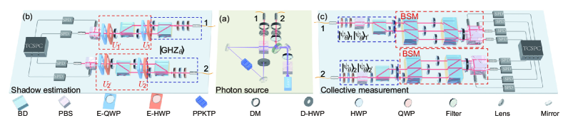
Figure 1: Schematic illustration of the experimental setup. (a) Generation of the biased polarization-entangled state $\cos\theta\ket{HH}_{12}+\sin\theta\ket{VV}_{12}$. (b) Setup to extend $\cos\theta\ket{HH}_{12}+\sin\theta\ket{VV}_{12}$ into $\ket{\text{GHZ}_{\theta}}=\cos\theta\ket{HhHh}_{11^{\prime}22^{\prime}}+\sin\theta\ket{VvVv}_{11^{\prime}22^{\prime}}$, and demonstrate the shadow estimation scheme. (c) Setup to prepare two-copy states and implement the collective measurement scheme. Symbols used in (a), (b), and (c) DM: dichroic mirror, E-HWP: electrically-rotated HWP, E-QWP: electrically-rotated quarter-wave plate, D-HWP: dual-wavelength HWP, TCSPC: time-correlated single-photon counting system.

Experimental quantification of entanglement and coherence—We use two efficient methods to experimentally detect the purity of photonic states and thus to bound the coherent information and relative entropy of coherence, respectively (Full details in Section 2 of  Not ). The first one is known as shadow estimation Huang et al. (2020); Chen et al. (2021); Struchalin et al. (2021). In shadow estimation, local random unitary operations $U_{n}\in\text{Cl}_{2}$ are individually applied on each qubit of an $N$-qubit state $\rho$, where $\text{Cl}_{2}$ is the single-qubit Clifford group. Then the rotated state is measured on the Pauli-$Z$ basis, producing a bit string $\ket{b}=\ket{b_{1}b_{2}\cdots b_{N}},b_{n}\in\{0,1\}$. The classical shadow of a single experimental run is constructed by $\hat{\rho}=\bigotimes_{n=1}^{N}3U_{n}^{\dagger}\ket{b_{n}}\bra{b_{n}}U_{n}-\mathbb{I}_{2}$ with $\mathbb{I}_{2}$ being identity matrix. By repeating the measurement $M$ times, one has a collection of classical shadows $\{\hat{\rho}^{(m)}\}$ which is further exploited for the estimation of various properties of the underlying state $\rho$ Elben et al. (2020); Brydges et al. (2019).

We implement shadow estimation on four-qubit biased Greenberger-Horne-Zeilinger (GHZ) states in the form of

$$\ket{\text{GHZ}_{\theta}}=\cos\theta\ket{0000}+\sin\theta\ket{1111}.$$ (7)

which are encoded on the polarization and path degrees of freedom (DOF) of photons. As shown in Fig. 1(a), the polarization-entangled photons are generated from a periodically poled potassium titanyl phosphate (PPKTP) crystal set at Sagnac interferometer with the ideal form of $\cos\theta\ket{HH}_{12}+\sin\theta\ket{VV}_{12}$, where $H$($V$) denotes the horizontal (vertical) polarization and $\theta$ is determined by the polarization of pump light. We then sent two photons into two beam displacers (BDs) as shown in Fig. 1(b), which transmits the vertical polarization and deviates the horizontal polarization. Consequently, the biased GHZ state $\ket{\text{GHZ}_{\theta}}=\cos\theta\ket{HhHh}_{11^{\prime}22^{\prime}}+\sin\theta\ket{VvVv}_{11^{\prime}22^{\prime}}$ is obtained, where $h$ ($v$) denotes the deviated (transmitted) spatial mode. The random unitary operations $U_{n}\in\text{Cl}_{2}$ on the polarization and path DOF are implemented with a combination of electrical-controlled half waveplate (E-HWP) and quarter waveplate (E-QWP) Zhang et al. (2021), and the projective measurements on the $Z$ basis are sequentially performed on the path and polarization DOF (See Not for more details).

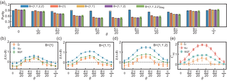
Figure 2: Experimental results of quantification of $I(A\rangle B)$ and $C_{\mathrm{RE}}$ on the prepared $\rho_{\text{GHZ}_{\theta}}$ by shadow estimation. (a) The estimation of global purity $\hat{\mathcal{P}}(\rho_{\text{GHZ}_{\theta}})$, marginal purity $\hat{\mathcal{P}}(\rho_{B})$ and the purity of diagonal matrix $\hat{\mathcal{P}}(\rho_{\text{GHZ}_{\theta,d}})$. The coloured bars represent the results from shadow estimation, while the black frames represent the results from SQT for comparison. (b)-(d) The upper bound $u_{e}$ and lower bound $l_{e}$ of $I(A\rangle B)$ with $B=\{1\}$, $B=\{1,1^{\prime}\}$ and $B=\{1,1^{\prime},2\}$ respectively. (e) The upper bound $u_{c}$ and lower bound $l_{c}$ of $C_{\mathrm{RE}}(\rho_{\text{GHZ}_{\theta}})$. The error bars represent the statistical error by repeating shadow estimation for 10 times.

We prepare eleven $\rho_{\text{GHZ}_{\theta}}$ by setting $\theta\in[0,\frac{\pi}{2}]$ with interval of $\frac{\pi}{20}$, and then use $M=2\times 10^{4}$ measurements in shadow estimation on each $\rho_{\text{GHZ}_{\theta}}$ to bound the coherent information $I(A\rangle B)$ of $\rho_{\text{GHZ}_{\theta}}$. We consider the bipartition of $\rho_{\text{GHZ}_{\theta}}$ with two subsystems $A$ and $B$, where $A\cup B=\left\{1,1^{\prime},2,2^{\prime}\right\}$ and $A\cap B=\varnothing$. Each subsystem contains $|A|$ and $|B|$ qubits, respectively. We consider three cases of $B=\{1\}$, $B=\{1,1^{\prime}\}$ and $B=\{1,1^{\prime},2\}$. The purities $\mathcal{P}_{\rho_{\text{GHZ}_{\theta}}}$ and $\mathcal{P}_{\rho_{B}}$ are estimated with $\{\hat{\rho}_{\text{GHZ}_{\theta}}^{(m)}\}$ by

$$\hat{\mathcal{P}}(\rho_{\text{GHZ}_{\theta}})=\frac{1}{M(M-1)}\sum_{m\neq m^{\prime}}\mathrm{Tr}\left[\hat{\rho}_{\text{GHZ}_{\theta}}^{(m)}\hat{\rho}_{\text{GHZ}_{\theta}}^{(m^{\prime})}\right]$$ (8)

and

$$\hat{\mathcal{P}}(\rho_{B})=\frac{1}{M(M-1)}\sum_{m\neq m^{\prime}}\mathrm{Tr}\left[\hat{\rho}_{B}^{(m)}\hat{\rho}_{B}^{(m^{\prime})}\right],$$ (9)

where $\hat{\rho}_{B}=\bigotimes_{n\in B}3U_{n}^{\dagger}\ket{b_{n}}\bra{b_{n}}U_{n}-\mathbb{I}_{2}$. The results of $\hat{\mathcal{P}}(\rho_{\text{GHZ}_{\theta}})$ and $\hat{\mathcal{P}}(\rho_{B})$ are shown in Fig. 2(a). To indicate the accuracy of estimated purities, we perform standard quantum tomography (SQT) Vogel and Risken (1989); Leonhardt (1995); White et al. (1999) on the prepared $\rho_{\text{GHZ}_{\theta}}$ with $1.4\times 10^{6}$ measurements, and treat the reconstructed state as target state. With the reconstructed $\rho_{\text{GHZ}_{\theta}}$, we calculate the corresponding purities that are shown with black frames in Fig. 2(a). The maximal error between purities (Eq. 8 and Eq. 9) estimated from classical shadows and SQT is $\epsilon=0.0132\pm 0.0109$. The high accuracy ($\epsilon\ll 1$) agrees well with theoretical prediction that the measurement cost of shadow tomography is the order of $2^{|AB|}/\epsilon^{2}$ Elben et al. (2020), while the SQT requires (at least) order of $2^{|AB|}\text{rank}(\rho_{AB})/\epsilon^{2}$ measurements to reach the same accuracy Haah et al. (2017); O’Donnell and Wright (2016). According to Eq. 3, the lower bound $l_{e}$ and upper bound $u_{e}$ of $I(A\rangle B)$ can be calculated with the estimated purities, and the results are shown with orange and blue dots in Fig. 2(b)-Fig. 2(d) respectively. We observe that $l_{e}>0$ with $\theta=\frac{3\pi}{20},\frac{4\pi}{20},\frac{5\pi}{20}$ and $\frac{6\pi}{20}$, which indicates the corresponding $\rho_{\text{GHZ}_{\theta}}$ admits distillable entanglement. The $I(A\rangle B)$ is also calculated with the reconstructed $\rho_{\text{GHZ}_{\theta}}$ and the results are shown with green dots in Fig. 2(b)-Fig. 2(d). The plots show that $I(A\rangle B)$) is tightly bounded by $l_{e}$ and $u_{e}$.

To bound $C_{\mathrm{RE}}(\rho_{\text{GHZ}_{\theta}})$, we calculate the purity of diagonal matrix of $\rho_{\text{GHZ}}$ by $\hat{\mathcal{P}}(\rho_{\text{GHZ}_{\theta,d}})=\sum_{i=1}^{16}{d_{i}^{2}}$ with $d_{i}$ being the diagonal elements of $\hat{\rho}_{\text{GHZ}_{\theta}}=\sum_{m=1}^{M}\hat{\rho}_{\text{GHZ}_{\theta}}^{(m)}$. The results of $\hat{\mathcal{P}}(\rho_{\text{GHZ}_{\theta,d}})$ are shown with blue bars in Fig. 2(a). Thus, $u_{c}$ and $l_{c}$ are deduced with estimated $\hat{\mathcal{P}}(\rho_{\text{GHZ}_{\theta,d}})$ and $\hat{\mathcal{P}}(\rho_{\text{GHZ}_{\theta}})$ according to Eq. 6. As $C_{\mathrm{RE}}\geq 0$, we set $l_{c}=0$ whenever it takes negative values. The results of calculated $u_{c}$ and $l_{c}$ are shown with red and yellow triangles in Fig. 2(e), in which one observes they tightly bound $C_{\text{RE}}(\rho_{\text{GHZ}_{\theta}})$ from SQT (cyan squares).

Next, we show that quantum resources can also be efficiently detected with collective measurements Yuan et al. (2020); Roik et al. (2022); Conlon et al. (2023), where $\mathcal{P}(\rho)$ is indicated from two copies of $\rho$ by $\mathcal{P}(\rho)={\rm Tr}(\rho^{2})={\rm Tr}(\mathbb{V}\rho\otimes\rho)$ with $\mathbb{V}$ being the swap operation on $\rho\otimes\rho$. We consider the case of two-qubit state in the form of $\ket{\psi_{2,\theta}}=\ket{\psi_{\theta}}_{1}\ket{\psi_{\theta}}_{2}$ with $\ket{\psi_{\theta}}_{1}=\ket{\psi_{\theta}}_{2}=\cos\theta\ket{0}+\sin\theta\ket{1}$. Experimentally, $\ket{\psi_{2,\theta}}$ is encoded in the polarization DOF and the setup to generate $\ket{\psi_{2,\theta}}$ as shown in Fig. 1(c). We first post-select the component $\ket{H}_{1}\ket{H}_{2}$ using two polarizing beam splitters (PBSs). By applying a HWP that transforms $\ket{H}$ to $\cos\theta\ket{H}+\sin\theta\ket{V}$ individually on photon 1 and photon 2, $\ket{\psi_{2,\theta}}$ is obtained. The copy of $\ket{\psi_{2,\theta}}$ is encoded in the path DOF, i.e., $\ket{\psi_{\theta}}_{1^{\prime}}=\ket{\psi_{\theta}}_{2^{\prime}}=\cos\theta\ket{h}+\sin\theta\ket{v}$.

The swap operation on $\mathbb{V}$ on $\rho\otimes\rho$ can be implemented by performing Bell-state measurement (BSM) between each qubit and its corresponding copy Moura Alves and Jaksch (2004); Islam et al. (2015); Girolami (2014). In our case, the BSM is performed between the polarization-encoded qubit $1(2)$ and the path-encoded qubit $1^{\prime}(2^{\prime})$ Li et al. (2021), respectively. The outcome probability of the two BSMs on $\rho_{12}\otimes\rho_{1^{\prime}2^{\prime}}$ is denoted by $p_{ij}=\mathrm{Tr}[(\Pi_{i}\otimes\Pi_{j})\rho_{\psi_{2,\theta}}\otimes\rho_{\psi_{2,\theta}}]$, where $\Pi_{1}=\ket{\Psi^{+}}\bra{\Psi^{+}}$, $\Pi_{2}=\ket{\Psi^{-}}\bra{\Psi^{-}}$, $\Pi_{3}=\ket{\Phi^{+}}\bra{\Phi^{+}}$, and $\Pi_{4}=\ket{\Phi^{-}}\bra{\Phi^{-}}$ are projectors onto Bell states $\ket{\Psi^{\pm}}=(\ket{Hv}\pm\ket{Vh})/\sqrt{2}$ and $\ket{\Phi^{\pm}}=(\ket{Hh}\pm\ket{Vv})/\sqrt{2}$. The purity of $\rho_{\psi_{2,\theta}}$ and the subsystem purity of $\rho_{\psi_{2,\theta,B}}$ with $B=\{2\}$ are then obtained by

$$\mathcal{P}(\rho_{\psi_{2,\theta}})=1-2(p_{12}+p_{32}+p_{42}+p_{21}+p_{23}+p_{24}),$$ (10)

and

$$\mathcal{P}(\rho_{\psi_{2,\theta,B}})=1-2(p_{12}+p_{22}+p_{32}+p_{42}).$$ (11)

Similarly, the purity of the diagonal matrix of $\rho_{\psi_{2,\theta}}$ can be obtained by

$$\mathcal{P}(\rho_{\psi_{2,\theta,d}})=1-2p_{33}+2p_{44}-p_{11}.$$ (12)

The results of $\mathcal{P}(\rho_{\psi_{2,\theta}})$, $\mathcal{P}(\rho_{\psi_{2,\theta,B}})$ and $\mathcal{P}(\rho_{\psi_{2,\theta,d}})$ are shown in Fig. 3(a), with $\theta\in[0,\frac{\pi}{2}]$ with interval of $\frac{\pi}{20}$. The lower bound $l_{e}$ and upper bound $u_{e}$ of $I(A\rangle B)$ are calculated according to Eq. 3 and shown in Fig. 3(b). We observe $u_{e}<0$ for all $\rho_{\psi_{2,\theta}}$, which indicates the prepared $\rho_{\psi_{2,\theta}}$ is less useful for entanglement distillation. Similarly, the lower bound $l_{c}$ and upper bound $u_{c}$ of $C_{\mathrm{RE}}(\ket{\psi_{2,\theta}})$ can be calculated according to Eq. 6. The results are shown in Fig. 3(c). Note that $l_{c}$ is much closer to $u_{c}$ compared to the case in Fig. 2(e). This is because the bounds $l_{c}$ and $u_{c}$ are functions of the leading order term (purity) in Taylor expansion of the von Neumann entropy about pure states, so that $l_{c}$ and $u_{c}$ are tight for pure states. Experimentally, the prepared $\rho_{12}$ and $\rho_{1^{\prime}2^{\prime}}$ are quite close to the ideal form of $\ket{\psi_{2,\theta}}$, while $\rho_{\text{GHZ}_{\theta}}$ is much more noisy. The high accuracy of $l_{c}$ and $u_{c}$ is also confirmed by $C_{\mathrm{RE}}(\rho_{12})$ with reconstructed $\rho_{12}$ from SQT, which is shown with cyan dots in Fig. 3(c).

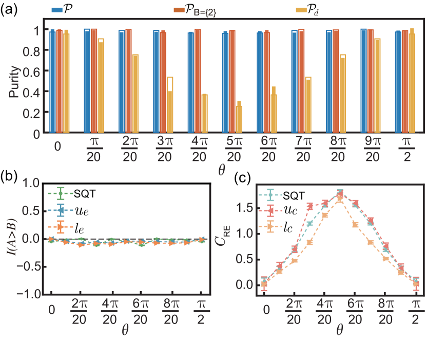
Figure 3: Experimental results of quantification of $I(A\rangle B)$ and $C_{\mathrm{RE}}$ of $\rho_{\psi_{2,\theta}}$ by collective measurements. (a) The estimated purities of $\mathcal{P}(\rho_{\psi_{2,\theta}})$, $\mathcal{P}(\rho_{\psi_{2,\theta,b}})$ and $\mathcal{P}(\rho_{\psi_{2,\theta,d}})$. (b) The upper bound $u_{e}$ and lower bound $l_{e}$ of $I(A\rangle B)$ with $B=\{2\}$. (c) The upper bound $u_{c}$ and lower bound $l_{c}$ of $C_{\mathrm{RE}}(\rho_{\psi_{2,\theta}})$. The error bars represent standard deviations obtained from conducting the experiment ten times.

Conclusion—We demonstrated universally valid, computable bounds to operationally meaningful measures of entanglement and coherence in terms of purity functionals. Then, we experimentally extracted these bounds by implementing two purity detection methods: shadow estimation and collective measurements. The first experiment showed that quantum resources can be estimated, rather than just witnessed, with precision that does not scale with the rank of the state, conversely to state tomography. The second one enabled to quantify coherence in non-entangled states. The scalability of the measurement network makes purity detection employable in testing the successful preparation of quantum superpositions in large computational registers, certifying that a complex device has run a truly quantum computation.

The results open several lines of investigation. First, the bounds Eqs. (2) and (5) represent the leading order term in Taylor’s expansion of the von Neumann entropy. We anticipate that tightened bounds can be extracted by evaluating the higher-order terms $\mathrm{Tr}(\rho^{3}),\mathrm{Tr}(\rho^{4}),\ldots,\mathrm{Tr}(\rho^{d})$, which can be efficiently detected with hybrid shadow estimation Zhou and Liu (2022). Secondly, one can extend the method proposed here to determine directly measurable bounds to the total correlations in multipartite systems $\{A_{i}\}$. For instance, consider the quantum analogue of the multi-information between random variables Han (1978); Modi et al. (2010)

$${\cal I}(\rho_{A_{1},\ldots,A_{n}})=\min\limits_{\bigotimes_{i}\sigma_{A_{i}}}S\left(\rho_{A_{1},\ldots,A_{n}}||\bigotimes_{i}\sigma_{A_{i}}\right).$$ (13)

It is easy to verify that the product of the state marginals $\bigotimes_{i}\rho_{A_{i}}$ solves the minimization, ${\cal I}(\rho_{A_{1},\ldots,A_{n}})=\sum_{i}S(\rho_{A_{i}})-S(\rho_{A_{1},\ldots,A_{n}})$. Quantitative bounds to the total system correlations in terms of purities are given by a straightforward generalization of Eq. 2.

Acknowledgments— We acknowledge T. Peng for the insightful discussions. This work is supported by the National Natural Science Foundation of China (Grants No. 11974213, No. 92065112 and No. 12175003), the National Key R&D Program of China (Grant No. 2019YFA0308200), Shandong Provincial Natural Science Foundation (Grants No. ZR2020JQ05), Taishan Scholar of Shandong Province (Grant No. tsqn202103013), Shenzhen Fundamental Research Program (Grant No. JCYJ20190806155211142), Shandong University Multidisciplinary Research and Innovation Team of Young Scholars (Grant No. 2020QNQT), the Higher Education Discipline Innovation Project (‘111’) (Grant No. B13029) and the High-performance Computing Platform of Peking University.

Supplementary Materials

.1 Derivation of the bounds

Given a quantum state $\rho$ in a $d$-dimensional Hilbert space, our task is to bound the Von Neumann entropy of $\rho$ with a function of the state purity $\mathcal{P}(\rho):=\mathrm{Tr}(\rho^{2}).$ The spectral decomposition of the quantum state is $\rho=\sum_{i=1}^{d}\lambda_{i}\ket{\psi_{i}}\bra{\psi_{i}}$, where $\{\ket{\psi_{i}}\}$ forms an orthonormal basis of the $d$-dimensional Hilbert space. The variational problem is then formulated as

$$\max/\min S(\rho) =-\sum_{i=1}^{d}\lambda_{i}\log(\lambda_{i})$$ (14)

$$s.t.{}{} \sum_{i=1}^{d}\lambda_{i}^{2}=\gamma$$

$$\sum_{i=1}^{d}\lambda_{i}=1$$

$$0\leq\lambda_{i}\leq 1,\forall i,$$

where $\mathcal{P}(\rho)=\mathrm{Tr}\rho^{2}$ is the purity of $\rho$.

Intuitively, the vector $\lambda$ that maximizes $S$ is the one that spread as uniformly as possible; while the vector $\lambda$ that minimizes $S$ is the one that has the minimal number of nonzero large values. In the following, we will analytically solve this problem and confirm this intuition.

.1.1 Maximization

First, we focus on the maximization problem with $d=3$. Note that when $d=2$, the solution to the constraints of Eq. 14 is unique and the optimization problem will be trivial. Without loss of generality, we assume $\lambda_{1}\geq\lambda_{2}\geq\lambda_{3}$. Then the problem can be stated as

$$\max S(\rho) =-\lambda_{1}\log(\lambda_{1})-\lambda_{2}\log(\lambda_{2})-\lambda_{3}\log(\lambda_{3})$$ (15)

$$s.t.{}{} \lambda_{1}^{2}+\lambda_{2}^{2}+\lambda_{3}^{2}=\gamma$$

$$\lambda_{1}+\lambda_{2}+\lambda_{3}=1$$

$$1\geq\lambda_{1}\geq\lambda_{2}\geq\lambda_{3}\geq 0.$$

We prove that the maximum is reached with the following Lemma.

Lemma 1.

The solution to the maximization problem in Eq. 15 is given by

$$\lambda_{1} =\frac{1}{3}+\sqrt{\frac{2}{3}\left(\mathcal{P}(\rho)-\frac{1}{3}\right)},$$ (16)

$$\lambda_{2} =\lambda_{3}=\frac{1-\lambda_{1}}{2}.$$

Proof.

The differential of the entropy function $S(\rho)$ and the constraints are given by

$$dS =-(1+\log\lambda_{1})d\lambda_{1}-(1+\log\lambda_{2})d\lambda_{2}-(1+\log\lambda_{3})d\lambda_{3}$$ (17)

and

$$\lambda_{1}d\lambda_{1}+\lambda_{2}d\lambda_{2}+\lambda_{3}d\lambda_{3}=0$$ (18)

$$d\lambda_{1}+d\lambda_{2}+d\lambda_{3}=0,$$

respectively. We rewrite Eq. 18 to

$$d\lambda_{1}= -\frac{(\lambda_{3}-\lambda_{2})}{\lambda_{1}-\lambda_{2}}d\lambda_{3},$$

$$d\lambda_{2}= -\frac{(\lambda_{1}-\lambda_{3})}{\lambda_{1}-\lambda_{2}}d\ \lambda_{3}.$$

Thus, the differential of the entropy function becomes

$$dS(\rho) =\frac{d\lambda_{3}}{\lambda_{1}-\lambda_{2}}[(\lambda_{3}-\lambda_{2})\log\lambda_{1}+(\lambda_{1}-\lambda_{3})\log\lambda_{2}$$ (19)

$$\quad+(\lambda_{2}-\lambda_{1})\log\lambda_{3}]$$

$$=(\lambda_{2}-\lambda_{3})\left[-\frac{\log\lambda_{1}-\log\lambda_{2}}{\lambda_{1}-\lambda_{2}}+\frac{\log\lambda_{3}-\log\lambda_{2}}{\lambda_{3}-\lambda_{2}}\right]d\lambda_{3}$$

Since the function $\log\lambda$ is concave for $\lambda\in[0,1]$, for $\lambda_{1}\geq\lambda_{2}\geq\lambda_{3}$,

$$\frac{\log\lambda_{1}-\log\lambda_{2}}{\lambda_{1}-\lambda_{2}}\leq\frac{\log\lambda_{3}-\log\lambda_{2}}{\lambda_{3}-\lambda_{2}}.$$

Thus, $dS(\rho)/d\lambda_{3}\geq 0$. To reach the maximum of $S(\rho)$, we thus only need to set $\lambda_{3}$ to be its maximum, which happens when $\lambda_{2}=\lambda_{3}$. Together with the constraints, then we can solve the equations and show that the solution to the maximization problem is given in Eq. 16. ∎

Now, we can solve the maximization problem of Eq. 14 for a general case of $d$.

Theorem 1.

Suppose $\lambda_{1}\geq\lambda_{2}\geq\dots\lambda_{d}$. The solution the solution to the maximization problem in Eq. 14 is

$$\lambda_{1} =\frac{1}{d}+\sqrt{\frac{d-1}{d}\left(\mathcal{P}(\rho)-\frac{1}{d}\right)},$$ (20)

$$\lambda_{2} =\lambda_{3}=\dots=\lambda_{d}=\frac{1-\lambda_{1}}{d-1}.$$

Proof.

The solution in Eq. 20 is exactly determined when setting $\lambda_{2}=\lambda_{3}=\dots=\lambda_{d}$. Suppose the maximization problem solution is not this one, then we must have that $\lambda_{2}>\lambda_{d}$. In the following, we prove the contradiction by showing that changing the values of $\lambda_{1},\lambda_{2},\lambda_{d}$ would make the entropy $S(\rho)$ larger while fixing all other values ($\lambda_{3},\lambda_{4},\dots,\lambda_{d-1}$) and the constraints. Now the constraints for $\lambda_{1}$, $\lambda_{2}$, and $\lambda_{d}$ becomes

$$\lambda_{1}^{2}+\lambda_{2}^{2}+\lambda_{d}^{2}=a$$ (21)

$$\lambda_{1}+\lambda_{2}+\lambda_{d}=b.$$

By defining $\lambda_{1}^{\prime}=\lambda_{1}/b$, $\lambda_{2}^{\prime}=\lambda_{2}/b$, $\lambda_{d}^{\prime}=\lambda_{d}/b$, the relations become

$$\lambda_{1}^{\prime 2}+\lambda_{2}^{\prime 2}+\lambda_{d}^{\prime 2} =a/b^{2}$$ (22)

$$\lambda_{1}^{\prime}+\lambda_{2}^{\prime}+\lambda_{d}^{\prime} =1.$$

The entropy function is

$$S(\rho) =-\sum_{i=1}^{d}\lambda_{i}\log(\lambda_{i}),$$ (23)

$$=S_{1,2,d}(\rho)+S_{r}(\rho),$$

where $S_{1,2,d}(\rho)=-\lambda_{1}\log(\lambda_{1})-\lambda_{2}\log(\lambda_{2})-\lambda_{d}\log(\lambda_{d})$ and $S_{r}(\rho)=-\sum_{i=3}^{d-1}\lambda_{i}\log(\lambda_{i})$. Since $S_{r}(\rho)$ is fixed, we need to maximize $S_{1,2,d}(\rho)$, which can also be represented as

$$S_{1,2,d}(\rho)=-b\lambda_{1}^{\prime}\log(b\lambda_{1}^{\prime})-b\lambda_{2}^{\prime}\log(b\lambda_{2}^{\prime})-b\lambda_{d}^{\prime}\log(b\lambda_{d}^{\prime})$$ (24)

$$=b[-\lambda_{1}^{\prime}\log(\lambda_{1}^{\prime})-\lambda_{2}^{\prime}\log(\lambda_{2}^{\prime})-\lambda_{d}^{\prime}\log(\lambda_{d}^{\prime})]-b\log b$$

Denoting $S_{1,2,d}^{\prime}(\rho)=-\lambda_{1}^{\prime}\log(\lambda_{1}^{\prime})-\lambda_{2}^{\prime}\log(\lambda_{2}^{\prime})-\lambda_{d}^{\prime}\log(\lambda_{d}^{\prime})$, this optimization problem has the same form of Eq. 15. Then Lemma 1 indicates that the maximum of $S_{1,2,d}^{\prime}(\rho)$ given the constraints in Eq. 22 is reached when $\lambda_{2}^{\prime}=\lambda_{d}^{\prime}$. In other words, the maximum of $S_{1,2,d}(\rho)$ given the constrains of Eq. 21 is saturated with $\lambda_{2}=\lambda_{d}$, which contradicts $\lambda_{2}>\lambda_{d}$. Therefore, the solution to the maximization problem is given by Eq. 20. ∎

.1.2 Minimization

Now, we consider the solution to the minimization of Eq. 14. Similarly, we first consider the minimization with $d=3$ and $\lambda_{1}\geq\lambda_{2}\geq\lambda_{3}$,

$$\min S(\rho) =-\lambda_{1}\log(\lambda_{1})-\lambda_{2}\log(\lambda_{2})-\lambda_{3}\log(\lambda_{3})$$ (25)

$$s.t.{}{} \lambda_{1}^{2}+\lambda_{2}^{2}+\lambda_{3}^{2}=\mathcal{P}(\rho)$$

$$\lambda_{1}+\lambda_{2}+\lambda_{3}=1$$

$$1\geq\lambda_{1}\geq\lambda_{2}\geq\lambda_{3}\geq 0.$$

Lemma 2.

The solution to the minimization problem in Eq. 25 is reached either when $\lambda_{1}=\lambda_{2}$ or $\lambda_{3}=0$.

Proof.

From the proof of Lemma 1, we already showed that $dS(\rho)/d\lambda_{3}\geq 0$. Therefore, the lower bound of $S(\rho)$ is reached when $\lambda_{3}$ takes its minimum. As $2(\lambda_{1}^{2}+\lambda_{2}^{2})\geq(\lambda_{1}+\lambda_{2})^{2}$, according to Eq. 25, we have

$$2(\mathcal{P}(\rho)-\lambda_{3}^{2})\geq(1-\lambda_{3})^{2}.$$ (26)

The lower bound for $\lambda_{3}$ is

$$\lambda_{3}\geq\max\left\{0,\frac{1-\sqrt{6\mathcal{P}(\rho)-2}}{3}\right\}$$

Thus, when $\mathcal{P}(\rho)\geq 1/2$, the minimal possible value for $\lambda_{3}$ is 0. When $1/3\leq\mathcal{P}(\rho)<1/2$, the minimal possible value for $\lambda_{3}$ is $\frac{1-\sqrt{6\mathcal{P}(\rho)-2}}{3}$ and $\lambda_{1}=\lambda_{2}=(1-\lambda_{3})/2$. Note that $\mathcal{P}(\rho)\geq 1/3$ for $d=3$. ∎

Now, we can show the general solution to the minimization of Eq. 14.

Theorem 2.

Suppose $\lambda_{1}\geq\lambda_{2}\geq\dots\lambda_{k}$, the solution to the minimization problem in Eq. 14 is

$$\lambda_{1}=\lambda_{2}=\dots=\lambda_{k-1} =\frac{1-\alpha}{k-1},$$ (27)

$$\lambda_{k} =\alpha,$$

$$\lambda_{k+1}=\dots=\lambda_{d} =0.$$

Here,

$$\alpha=\frac{1}{k}-\sqrt{(1-1/k)(\mathcal{P}(\rho)-1/k)}$$ (28)

and $k$ is the integer such that $\frac{1}{k}\leq\mathcal{P}(\rho)\leq\frac{1}{k-1}$.

Proof.

Suppose we always have the solution in the form as

$$\lambda_{1}=\lambda_{2}=\dots=\lambda_{k-1},\lambda_{k},\lambda_{k+1}=\dots\lambda_{d}=0.$$ (29)

Otherwise, there must exist three $\lambda_{i},\lambda_{j},\lambda_{k}$ such that $\lambda_{i}>\lambda_{j}\geq\lambda_{k}$ and $\lambda_{k}\neq 0$. Following a similar argument in the proof of Theorem 1, we can show that this contradicts Lemma 2.

According to Eq. 29, we have

$$(k-1)\lambda_{1}^{2}+\lambda_{k}^{2} =\mathcal{P}(\rho),$$

$$(k-1)\lambda_{1}+\lambda_{k} =1,$$

$$k \leq d$$

We can show that the possible integer value for $k$ is unique. That is,

$$k[(k-1)\lambda_{1}^{2}+\lambda_{k}^{2}] \geq[(k-1)\lambda_{1}+\lambda_{k}]^{2}$$

$$\geq(k-1)[(k-1)\lambda_{1}^{2}+\lambda_{k}^{2}]$$

Equivalently, we have

$$k\mathcal{P}(\rho)\geq 1\geq(k-1)\mathcal{P}(\rho),$$

hence

$$\frac{1}{\mathcal{P}(\rho)}\leq \,\,k\,\,\leq\frac{1}{\mathcal{P}(\rho)}+1,$$

$$\frac{1}{k}\leq \,\,\mathcal{P}(\rho)\,\,\leq\frac{1}{k-1}.$$

∎

.1.3 Upper and lower bounds to coherence and entanglement

We now call $\{\lambda_{i,\rho}^{\text{M}}\},\{\lambda_{i,\rho}^{\text{m}}\}$ the vectors solving the maximization and the minimization, respectively. Given a bipartite state $\rho_{AB}$, by minimizing (maximizing) the marginal purity on $B$ subsystem and maximizing (minimizing) the global purity, one has
Result 1 ( Eq. 2 of the main text)— Given a quantum state $\rho_{AB}\in\mathcal{H}_{d_{A}}\otimes\mathcal{H}_{d_{B}}$, and defining $\rho_{B}=\mathrm{Tr}_{A}\rho_{AB}$, its coherent information $I(A\rangle B)$ is bounded as follows:

$$l_{e}(\rho_{AB})\leq I(A\rangle B)\leq u_{e}(\rho_{AB}),$$ (30)

$$l_{e}(\rho_{AB})=$$

$$- (1-\lambda^{\text{m}}_{k_{\rho_{B}},\rho_{B}})\log\lambda^{\text{m}}_{1,\rho_{B}}-\lambda^{\text{m}}_{k_{\rho_{B}},\rho_{B}}\log\lambda^{\text{m}}_{k_{\rho_{B}},\rho_{B}}$$

$$+ (1-\lambda^{\text{M}}_{1,\rho_{AB}})\log\frac{(1-\lambda^{\text{M}}_{1,\rho_{AB}})}{(d-1)}+\lambda^{\text{M}}_{1,\rho_{AB}}\log{\lambda^{\text{M}}_{1,\rho_{AB}}},$$

$$u_{c}(\rho_{AB})=$$

$$(1-\lambda^{\text{m}}_{k_{\rho_{AB}},\rho_{AB}})\log\lambda^{\text{m}}_{1,\rho_{AB}}+\lambda^{\text{m}}_{k_{\rho_{AB}},\rho_{AB}}\log\lambda^{\text{m}}_{k_{\rho_{AB}},\rho_{AB}}$$

$$- (1-\lambda^{\text{M}}_{1,\rho_{B}})\log\frac{(1-\lambda^{\text{M}}_{1,\rho_{B}})}{(d_{B}-1)}-\lambda^{\text{M}}_{1,\rho_{B}}\log\lambda^{\text{M}}_{1,\rho_{B}}.$$

By minimizing (maximizing) the coherence of the dephased state $\rho_{d}=\sum_{i}\ket{i}\!\!\bra{i}\rho\ket{i}\!\!\bra{i}$, and maximizing (minimizing) the coherence of the state under study, we obtain lower (upper) bounds to the relative entropy of coherence:
Result 2 ( Eq. 5 of the main text) — The relative entropy of coherence $C_{\mathrm{RE}}(\rho)$ is bounded as follows:

$$l_{c}(\rho)\leq C_{\mathrm{RE}}(\rho)\leq u_{c}(\rho),$$ (31)

$$l_{c}(\rho)=-(1-\lambda^{\text{m}}_{k_{\rho_{d}},\rho_{d}})\log\lambda^{\text{m}}_{1,\rho_{d}}-\lambda^{\text{m}}_{k_{\rho_{d}},\rho_{d}}\log\lambda^{\text{m}}_{k_{\rho_{d}},\rho_{d}}$$

$$+ (1-\lambda^{\text{M}}_{1,\rho})\log\frac{(1-\lambda^{\text{M}}_{1,\rho})}{(d-1)}+\lambda^{\text{M}}_{1,\rho}\log{\lambda^{\text{M}}_{1,\rho}},$$

$$u_{c}(\rho)=(1-\lambda^{\text{m}}_{k_{\rho},\rho})\log\lambda^{\text{m}}_{1,\rho}+\lambda^{\text{m}}_{k_{\rho},\rho}\log\lambda^{\text{m}}_{k_{\rho},\rho}$$

$$- (1-\lambda^{\text{M}}_{1,\rho_{d}})\log\frac{(1-\lambda^{\text{M}}_{1,\rho_{d}})}{(d-1)}-\lambda^{\text{M}}_{1,\rho_{d}}\log\lambda^{\text{M}}_{1,\rho_{d}}.$$

.2 Details of experimental realizations and results

Before discussing the experimental details, we provide an overview of the crucial optical components and their respective functions employed in our experiment:

• Waveplates: We utilize both half-wave plates (HWPs) and quarter-wave plates (QWPs) to perform unitary operations ($U$) on photons. The angle between the fast axis of the waveplate and the vertical polarization direction is denoted as $\omega$ for HWPs and $\vartheta$ for QWPs. These waveplates induce specific unitary transformations on the quantum state of photons, enabling the desired experimental operations. The unitary transformations of HWPs and QWPs can be expressed as:

  $$U_{\text{HWP}}(\omega) =-\begin{pmatrix}\cos 2\omega&\sin 2\omega\\ \sin 2\omega&-\cos 2\omega\\ \end{pmatrix},$$ (32)

  $$U_{\text{QWP}}(\vartheta) =\frac{1}{\sqrt{2}}\begin{pmatrix}1+i\cos 2\vartheta&i\sin 2\vartheta\\ i\sin 2\vartheta&1-i\cos 2\vartheta\\ \end{pmatrix}$$ (33)

• Polarization beam splitter (PBS): This component separates photons with perpendicular polarization directions. It transmits horizontally polarized photons while reflecting vertically polarized photons.

• Beam displacer (BD): The BD allows vertically polarized photons to pass through in the original direction, while horizontally polarized photons are displaced. In our experiment, we use a BD with a length of 28.3 mm, resulting in a displacement offset of 3 mm.

.2.1 Biased polarization-entangled photon source

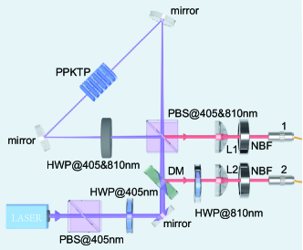
Figure 5: Schematic illustration of biased polarization-entangled photon source.

We use a continuous-wave laser operating at a central wavelength of 405 nm with a full width at half maximum (FWHM) of 0.012 nm as our pump light source Fig. 5. The pump light passes through a PBS followed by an HWP set at $\theta/2$, which transforms the polarization of the pump light into $\cos\theta\ket{H}_{p}+\sin\theta\ket{V}_{p}$. The pump light passes PBS that transmits the component of $\ket{H}$ and reflects component of $\ket{V}$. Then, the periodically poled potassium titanyl phosphate (PPKTP) is coherently pumped from anticlockwise and clockwise directions respectively, and the generated photons are superposed on the PBS leading to the outcome state of $\cos\theta\ket{HV}_{12}+\sin\theta\ket{VH}_{12}$. An HWP set at $45^{\circ}$ is applied on photon 2, which leads to a biased polarization-entangled state in form of $\cos\theta\ket{HH}_{12}+\sin\theta\ket{VV}_{12}$

To enhance collective efficiency, we employ lens L1 with a focal length of 200 mm and lens L2 with a focal length of 250 mm. The two photons pass through narrowband filters (NBFs) with an FWHM of 3 nm and then are coupled into single-mode fibres.

.2.2 Preparation of $\ket{\text{GHZ}_{\theta}}$ and $\ket{\psi_{2,\theta}}$

To generate $\ket{\text{GHZ}_{\theta}}$, photon 1 and 2 pass through two BDs after calibration of their polarization as shown in Fig. 6(a). Calling $h(v)$ the deviated (transmitted) spatial modes, the step-by-step description of optical elements to generate $\ket{\text{GHZ}_{\theta}}$ is

$$\cos\theta\ket{HH}_{12}+\sin\theta\ket{VV}_{12}$$ (34)

$$\xrightarrow{\rm{BD1}} \cos\theta\ket{HhH}_{11^{\prime}2}+\sin\theta\ket{VvV}_{11^{\prime}2}$$

$$\xrightarrow{\rm{BD2}} \cos\theta\ket{HhHh}_{11^{\prime}22^{\prime}}+\sin\theta\ket{VvVv}_{11^{\prime}22^{\prime}}.$$

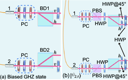
Figure 6: (a) The setup to generate biased four-qubit GHZ states $\ket{\text{GHZ}_{\theta}}$. (b) The setup to generate two-copy states $\ket{\psi_{2,\theta}}$. PC: polarization control is a combination of QWP, HWP and QWP which can be set to calibrate the variation of polarization caused by the twist of fibre.

In the experiment, by changing the value of $\theta$, we totally generate eleven $\rho_{\text{GHZ}_{\theta}}$. For each $\rho_{\text{GHZ}_{\theta}}$, we reconstruct the corresponding density matrix $\rho_{\text{GHZ}_{\theta}}$ using standard quantum state tomography (SQT). We calculate the fidelity $F={\rm Tr}(\rho_{\text{GHZ}_{\theta}}\ket{\text{GHZ}_{\theta}}\bra{\text{GHZ}_{\theta}})$. The results are summarized in Table 1.

Table 1: The fidelities of the prepared $\rho_{\text{GHZ}_{\theta}}$.

$\theta$	$F$
0	$0.9293\pm 0.0004$
$\pi/20$	$0.9050\pm 0.0006$
$2\pi/20$	$0.9057\pm 0.0007$
$3\pi/20$	$0.9331\pm 0.0005$
$4\pi/20$	$0.9136\pm 0.0006$
$5\pi/20$	$0.9124\pm 0.0007$
$6\pi/20$	$0.9155\pm 0.0003$
$7\pi/20$	$0.8850\pm 0.0007$
$8\pi/20$	$0.8833\pm 0.0009$
$9\pi/20$	$0.9155\pm 0.0005$
$10\pi/20$	$0.9290\pm 0.0004$

The setup to prepare $\ket{\psi_{2,\theta}}\otimes\ket{\psi_{2,\theta}}$ is illustrated in Fig. 6(b). Photon 1 and 2 pass through two PBSs creating the resulting state of $\ket{HH}_{12}$. The step-by-step description of optical elements to generate $\ket{\psi_{2,\theta}}\otimes\ket{\psi_{2,\theta}}$ is

$$\ket{HH}_{12} \xrightarrow[\text{are applied on photon 1 and 2}]{\text{Two HWPs}@\theta/2}(\cos\theta\ket{H}_{1}+\sin\theta\ket{V}_{1})\otimes(\cos\theta\ket{H}_{2}+\sin\theta\ket{V}_{2})$$ (35)

$$\xrightarrow[\text{are applied on photon 1 and 2}]{\rm{BD1}\&\rm{BD2}}(\cos\theta\ket{Hh}_{11^{\prime}}+\sin\theta\ket{Vv}_{11^{\prime}})\otimes(\cos\theta\ket{Hh}_{22^{\prime}}+\sin\theta\ket{Vv}_{22^{\prime}})$$

$$\xrightarrow[\text{are applied on path}\,\,h\,\,\text{of photon 1 and 2}]{\text{Two HWPs}@45\degree}\ket{VV}_{12}\otimes[(\cos\theta\ket{h}_{1^{\prime}}+\sin\theta\ket{v}_{1^{\prime}})\otimes(\cos\theta\ket{h}_{2^{\prime}}+\sin\theta\ket{v}_{2^{\prime}})]=\ket{VV}_{12}\otimes\ket{\psi_{2,\theta}}_{1^{\prime}2^{\prime}}$$

$$\xrightarrow[\text{are applied on both path of photon 1 and 2}]{\text{Two HWPs}@\theta/2}\ket{\psi_{2,\theta}}_{12}\otimes\ket{\psi_{2,\theta}}_{1^{\prime}2^{\prime}}$$

As shown in Eq. 35, the first $\ket{\psi_{2,\theta}}$ is encoded into the polarization degree of freedom (DOF) of both photons, while the second $\ket{\psi_{2,\theta}}$ is encoded on the path DOF of both photons.

.2.3 Experimental setups to perform shadow estimation and collective measurements

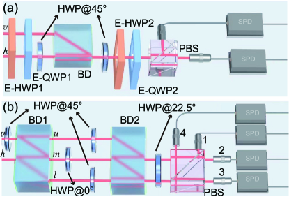
Figure 7: Illustration of setups to perform (a) shadow estimation and (b) collective measurements.

In shadow estimation, the single-qubit Clifford unitary operation $U_{n}\in\text{Cl}_{2}$ followed by a projective measurement on Pauli-Z basis is equivalent to measuring qubit on basis $J_{n}=U_{n}^{\dagger}ZU_{n}\in\left\{\pm X,\pm Y,\pm Z\right\}$. The experimental setup to perform measurement on arbitrary basis $(\alpha\ket{H}+\delta\ket{V})\otimes(\gamma\ket{h}+\mu\ket{v})$ is shown in Fig. 7(a), where $\alpha\ket{H}+\delta\ket{V}$ is encoded on polarization DOF and $\gamma\ket{h}+\mu\ket{v}$ is encoded on path DOF. Projection on $\alpha\ket{H}+\delta\ket{V}$ is realized by combination of E-HWP1 (set at angle of $\theta_{1}$) and E-QWP1 (set at angle of $\upsilon_{1}$), while the projection of $\gamma\ket{h}+\mu\ket{v}$ and its orthogonal basis is realized by combination of E-HWP2 (set at angle of $\theta_{2}$), E-QWP2 (set at angle of $\upsilon_{2}$) and a PBS. A step-by-step description of implementation of such projective measurement is described by

$$(\alpha\ket{H}+\beta\ket{V})\otimes(\gamma\ket{h}+\delta\ket{v}) \xrightarrow[\text{on both path}]{\text{E-HWP1}@\omega_{1}\&\text{E-QWP1}@\vartheta_{1}}\ket{H}\otimes(\gamma\ket{h}+\delta\ket{v})$$ (36)

$$\xrightarrow[\rm{on\,\,path\,\,}h]{\text{HWP}@45^{\circ}}\gamma\ket{Vh}+\delta\ket{Hv}$$

$$\xrightarrow[\text{combine the path}\,\,h\,\,\text{and}\,\,v]{\rm{BD3}}\gamma\ket{V}+\delta\ket{H}$$

$$\xrightarrow{\rm{HWP@45^{\circ}}}\gamma\ket{H}+\delta\ket{V}$$

$$\xrightarrow[]{\text{E-HWP2}@\omega_{2}\&\text{E-QWP2}@\vartheta_{2}}\ket{H}$$

$$\xrightarrow{\rm{PBS}}\left\{\begin{array}[]{rcl}\text{transmitted},&\text{results of}\,\,(\alpha\ket{H}+\beta\ket{V})\otimes(\gamma\ket{h}+\delta\ket{v})\\ \text{reflected},&\text{results of}\,\,(\alpha\ket{H}+\beta\ket{V})\otimes(\gamma\ket{h}+\delta\ket{v})^{\perp}\end{array},\right.$$

where $(\gamma\ket{h}+\delta\ket{v})^{\perp}$ is the orthogonal state of $\gamma\ket{h}+\delta\ket{v}$.

The experimental setup to implement BSM between polarization-encoded qubit and path-encoded qubit is shown in Fig. 7(b). Note that the projection on four Bell states is demonstrated with single experimental setting. A detailed description of Fig. 7(b) is

$$\begin{split}&\begin{cases}&\ket{\Psi^{+}}=\frac{1}{\sqrt{2}}(\ket{Hv}+\ket{Vh})\\ &\ket{\Psi^{-}}=\frac{1}{\sqrt{2}}(\ket{Hv}-\ket{Vh})\\ &\ket{\Phi^{+}}=\frac{1}{\sqrt{2}}(\ket{Hh}+\ket{Vv})\\ &\ket{\Phi^{-}}=\frac{1}{\sqrt{2}}(\ket{Hh}-\ket{Vv})\\ \end{cases}\xrightarrow[\text{on path}\,\,v]{\text{HWP}@45^{\circ}}\begin{cases}&\frac{1}{\sqrt{2}}(\ket{Vv}+\ket{Vh})\\ &\frac{1}{\sqrt{2}}(\ket{Vv}-\ket{Vh})\\ &\frac{1}{\sqrt{2}}(\ket{Hh}+\ket{Hv})\\ &\frac{1}{\sqrt{2}}(\ket{Hh}-\ket{Hv})\\ \end{cases}\xrightarrow[\text{Re-encoding}]{\text{BD1}}\begin{cases}&\frac{1}{\sqrt{2}}(\ket{Vu}+\ket{Vm})\\ &\frac{1}{\sqrt{2}}(\ket{Vu}-\ket{Vm})\\ &\frac{1}{\sqrt{2}}(\ket{Hl}+\ket{Hm})\\ &\frac{1}{\sqrt{2}}(\ket{Hl}-\ket{Hm})\\ \end{cases}\\ &\xrightarrow[\text{HWP}@0^{\circ}\text{on path}\,\,m]{\text{HWPs}@45^{\circ}\text{on path}\,\,u\,\,\text{and}\,\,l}\begin{cases}&\frac{1}{\sqrt{2}}(\ket{Hu}-\ket{Vm})\\ &\frac{1}{\sqrt{2}}(\ket{Hu}+\ket{Vm})\\ &\frac{1}{\sqrt{2}}(\ket{Vl}+\ket{Hm})\\ &\frac{1}{\sqrt{2}}(\ket{Vl}-\ket{Hm})\\ \end{cases}\xrightarrow[\text{combine path}]{\text{BD2}}\begin{cases}&\ket{-}\ket{m}\\ &\ket{+}\ket{m}\\ &\ket{+}\ket{l}\\ &\ket{-}\ket{l}\\ \end{cases}\xrightarrow[\text{on path}\,\,m\,\,\text{and}\,\,l]{\text{HWP}@22.5^{\circ}}\begin{cases}&\ket{V}\ket{m}\\ &\ket{H}\ket{m}\\ &\ket{H}\ket{l}\\ &\ket{V}\ket{l}\\ \end{cases}\xrightarrow[]{\text{PBS}}\begin{cases}&\text{clicks on detector 1}\\ &\text{clicks on detector 2}\\ &\text{clicks on detector 3}\\ &\text{clicks on detector 4}\\ \end{cases}.\end{split}$$ (37)

References

Nielsen and Chuang (2011)M. A. Nielsen and I. L. Chuang, “Quantum computation
and quantum information,” (2011).
Giovannetti et al. (2011)V. Giovannetti, S. Lloyd,
and L. Maccone, Nature photonics 5, 222 (2011).
Zhang et al. (2019)C. Zhang, T. R. Bromley,
Y.-F. Huang, H. Cao, W.-M. Lv, B.-H. Liu, C.-F. Li, G.-C. Guo, M. Cianciaruso, and G. Adesso, Phys. Rev. Lett. 123, 180504 (2019).
Lostaglio et al. (2015)M. Lostaglio, D. Jennings,
and T. Rudolph, Nature
communications 6, 6383
(2015).
Narasimhachar and Gour (2015)V. Narasimhachar and G. Gour, Nature
communications 6, 7689
(2015).
Romero et al. (2014)E. Romero, R. Augulis,
V. I. Novoderezhkin,
M. Ferretti, J. Thieme, D. Zigmantas, and R. Van Grondelle, Nature physics 10, 676 (2014).
Huelga and Plenio (2013)S. F. Huelga and M. B. Plenio, Contemporary Physics 54, 181 (2013).
Lloyd (2011)S. Lloyd, in Journal of
Physics-Conference Series, Vol. 302 (2011) p. 012037.
Lambert et al. (2013)N. Lambert, Y.-N. Chen,
Y.-C. Cheng, C.-M. Li, G.-Y. Chen, and F. Nori, Nature Physics 9, 10 (2013).
Brydges et al. (2019)T. Brydges, A. Elben,
P. Jurcevic, B. Vermersch, C. Maier, B. P. Lanyon, P. Zoller, R. Blatt, and C. F. Roos, Science 364, 260 (2019).
Elben et al. (2022)A. Elben, S. T. Flammia,
H.-Y. Huang, R. Kueng, J. Preskill, B. Vermersch, and P. Zoller, Nature Reviews Physics , 1 (2022).
Elben et al. (2020)A. Elben, R. Kueng,
H.-Y. R. Huang, R. van Bijnen, C. Kokail, M. Dalmonte, P. Calabrese, B. Kraus, J. Preskill, P. Zoller, and B. Vermersch, Phys. Rev. Lett. 125, 200501 (2020).
Wu et al. (2021)K.-D. Wu, A. Streltsov,
B. Regula, G.-Y. Xiang, C.-F. Li, and G.-C. Guo, Advanced Quantum Technologies 4, 2100040 (2021).
Zhang et al. (2017)C. Zhang, B. Yadin,
Z.-B. Hou, H. Cao, B.-H. Liu, Y.-F. Huang, R. Maity, V. Vedral, C.-F. Li, G.-C. Guo, and D. Girolami, Phys. Rev. A 96, 042327 (2017).
Hou et al. (2018)Z. Hou, J.-F. Tang,
J. Shang, H. Zhu, J. Li, Y. Yuan, K.-D. Wu, G.-Y. Xiang, C.-F. Li, and G.-C. Guo, Nature
communications 9, 1414
(2018).
Wu et al. (2019)K.-D. Wu, Y. Yuan, G.-Y. Xiang, C.-F. Li, G.-C. Guo, and M. Perarnau-Llobet, Science Advances 5, eaav4944 (2019).
Huang et al. (2020)H.-Y. Huang, R. Kueng, and J. Preskill, Nature Physics 16, 1050 (2020).
Aaronson (2020)S. Aaronson, SIAM
Journal on Computing 49, STOC18 (2020).
Yuan et al. (2020)Y. Yuan, Z. Hou, J.-F. Tang, A. Streltsov, G.-Y. Xiang, C.-F. Li, and G.-C. Guo, npj Quantum Information 6, 1 (2020).
Roik et al. (2022)J. Roik, K. Bartkiewicz,
A. Černoch, and K. Lemr, Physics Letters A 446, 128270 (2022).
Conlon et al. (2023)L. O. Conlon, T. Vogl,
C. D. Marciniak, I. Pogorelov, S. K. Yung, F. Eilenberger, D. W. Berry, F. S. Santana, R. Blatt, T. Monz, et al., Nature Physics , 1
(2023).
Zhou and Liu (2022)Y. Zhou and Z. Liu, “A hybrid framework for estimating
nonlinear functions of quantum states,” (2022), arXiv:2208.08416 [quant-ph]
.