Efficient Characterizations of Multiphoton States with Ultra-thin Integrated Photonics

Abstract

Metasurface enables the generation and manipulation of multiphoton entanglement with flat optics, providing a more efficient platform for large-scale photonic quantum information processing. Here, we show that a single metasurface optical chip would allow more efficient characterizations of multiphoton entangled states, such as shadow tomography, which generally requires fast and complicated control of optical setups to perform projective measurements in different bases, a demanding task using conventional optics. The compact and stable device here allows implementations of general positive observable value measures with a reduced sample complexity and significantly alleviates the experimental complexity to implement shadow tomography. Integrating self-learning and calibration algorithms, we observe notable advantages in the reconstruction of multiphoton entanglement, including using fewer measurements, having higher accuracy, and being robust against optical loss. Our work unveils the feasibility of metasurface as a favorable integrated optical device for efficient characterization of multiphoton entanglement, and sheds light on scalable photonic quantum technologies with ultra-thin integrated optics.

Metasurface, an ultra-thin and highly integrated optical device, is capable of full light control and thus provides novel applications in quantum photonics Solntsev et al. (2021). In photonic quantum information processing, multiphoton entanglement is the building block for wide range of tasks, such as quantum computation Walther et al. (2005), quantum error correction Yao et al. (2012), quantum secret sharing Bell et al. (2014); Lu et al. (2016), and quantum sensing Liu et al. (2021). Recent investigations highlighted the feasibility of metasurface in generations Li et al. (2020); Santiago-Cruz et al. (2022), manipulations Georgi et al. (2019); Li et al. (2021); Zhang et al. (2022), and detections Wang et al. (2018, 2022) of multiphoton entanglement, indicating metasurface as a promising technology of ultra-thin integrated optics for large-scale quantum information processing.

The characterization of multiphoton entanglement provides diagnostic information on experimental imperfections and benchmarks our technological progress towards the reliable control of large-scale photons. The standard quantum tomography (SQT) James et al. (2001a) requires an exponential overhead with respect to the system size. Recently, more efficient protocols have been proposed and demonstrated with fewer measurements, such as compressed sensing Gross et al. (2010); Liu et al. (2012), adaptive tomography Mahler et al. (2013); Hou et al. (2016); Granade et al. (2017) and self-guided quantum tomography (SGQT) Ferrie (2014); Chapman et al. (2016); Rambach et al. (2021). Apart from state reconstruction, an alternative scheme, known as shadow tomography Aaronson (2018); Huang et al. (2020), has been proposed to more efficiently predict functions of the quantum states. Nevertheless, these advanced approaches generally require the experimental capability of performing either measurements on different bases or applying complex unitary rotations, leading to the consequence that the manipulation time is much longer than the time of data acquisition. A potential solution is to replace the unitary operations and projective measurements with positive operator valued measures (POVMs), which is capable to extract complete information in a single experimental setting Acharya et al. (2021); Stricker et al. (2022); Nguyen et al. (2022). However, a compact and scalable implementation of POVM in optical system is still technically changeling.

In this work, we report an implementation of POVM enabled by a metasurface, which is based on planar arrays of nanopillars and able to provide complete control of polarization. The POVM we achieved allows to implement real-time shadow tomography, and observe the shadow norm that determines sample complexity. Moreover, we show that the metasurface-enabled shadow tomography can be readily incorporated the original proposal Huang et al. (2020) with other algorithms, including the simultaneous perturbation stochastic approximation (SPSA) Spall (1992) to return a physical state and robust shadow tomography Chen et al. (2021) against experimental imperfections. With these improvements, we observe the unexplored advantages of shadow tomography in terms of fewer measurements required, higher accuracy of reconstruction, and robustness against the engineered optical loss.

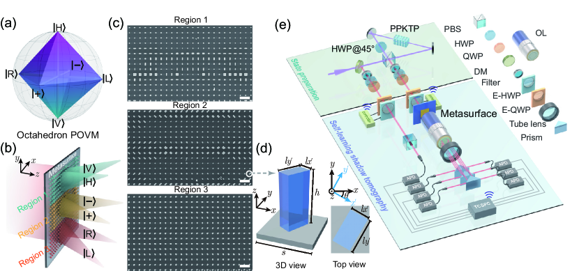
Figure 1: Concept of metasurface-enabled POVM and experimental setup to perform shadow tomography. (a), The elements in $\mathbf{E}_{\text{octa}}$ are projectors on states $|H\rangle$, $|V\rangle$, $|+\rangle$, $|-\rangle$, $|R\rangle$ and $|L\rangle$ respectively, which forms a symmetric polytope of an octahedron on Bloch sphere. (b), The metasurface to realize $\mathbf{E}_{\text{octa}}$, green, yellow and red blocks on the metasurface represent nanopillars with different arrangement. (c), The scanning electron microscopy images of the fabricated nanopillars in three regions. (d), Schematic drawing of single nanopillar that is fabricated with same height of 700nm but different $(\theta,l_{x^{\prime}},l_{y\prime})$. (e), Setup to generate entangled photons and demonstrate self-learning shadow tomography with metasurface. PBS: polarizing beam splitter. DM: dichroic mirror. HWP: half-wave plate. QWP: quarter-wave plate. E-HWP: electrically-rotated HWP. E-QWP: electrically-rotated QWP. OL: objective lens.

We first briefly review the shadow tomography with POVM. Considering a 2-level (qubit) quantum system, a set of $L$ rank-one projectors $\{|\psi_{l}\rangle\langle\psi_{l}|\in\mathbb{H}_{2}\}_{l=1}^{L}$ is called a quantum 2-design if the average value of the second-moment operator $(|\psi_{l}\rangle\langle\psi_{l}|)^{\otimes 2}$ over the set is proportional to the symmetric subspace of two copies Guţă et al. (2020). Each quantum 2-design is proportional to a POVM $\mathbf{E}=\{\frac{2}{L}|\psi_{l}\rangle\langle\psi_{l}|\}_{l=1}^{L}$ with the element $E_{l}=\frac{2}{L}|\psi_{l}\rangle\langle\psi_{l}|$ being positive semidefinite and satisfying $\sum_{l=1}^{L}E_{l}=\mathds{1}_{2}$. Measuring a quantum state $\rho$ using POVM $\mathbf{E}$ results one $l\in[L]$ outcome with probability ${\rm Pr}(l|\rho)={\rm Tr}(E_{l}\rho)$ according to Born’s rule. The POVM $\mathbf{E}$ together with the preparation of the corresponding state $|\psi_{l}\rangle$ can be viewed as a linear map $\mathcal{M}:\mathbb{H}_{2}\to\mathbb{H}_{2}$, and the ‘classical shadow’ is the solution of least-square estimator with single experimental run,

$$\hat{\rho}^{(m)}_{l}=\mathcal{M}^{-1}(|\psi_{l}\rangle\langle\psi_{l}|)=3|\psi_{l}\rangle\langle\psi_{l}|-\mathds{1}_{2}.$$ (1)

For an $N$-qubit state, the classical shadow is the tensor product of simultaneous single-qubit estimations $\hat{\rho}^{(m)}=\bigotimes_{n=1}^{N}\hat{\rho}^{(m)}_{l_{n}}$ with $l_{n}$ the outcome of $n$-th qubit, and one has $\mathbb{E}[\hat{\rho}^{(m)}]=\rho$. Repeating the POVM $M$ times, one has a collection of classical shadows $\{\hat{\rho}^{(m)}\}_{m=1}^{M}$, which is further inquired for estimation of various properties of the underlying state.

In our experiment, we focus on the POVM on polarization-encoded photonic qubit, i.e., $|0(1)\rangle=|H(V)\rangle$ with $|H(V)\rangle$ being the horizontal (vertical) polarization, and consider POVM of $L=6$ and $|\psi_{l}\rangle\in\{|H\rangle,|V\rangle,|+\rangle,|-\rangle,|L\rangle,|R\rangle\}$ with $|\pm\rangle=(|H\rangle\pm|V\rangle)/\sqrt{2}$ and $|L(R)\rangle=(|H\rangle\pm i|V\rangle)/\sqrt{2}$. The corresponding POVM $\mathbf{E}_{\text{octa}}$ is described by a symmetric polytope of an octahedron on Bloch sphere as shown in Figure 1(a). To realize $\mathbf{E}_{\text{octa}}$, we design and fabricate a 210$\mu$m$\times$210$\mu$m polarization-dependent metasurface that splits incident light into six directions corresponding to projection on $|H\rangle$, $|V\rangle$, $|+\rangle$, $|-\rangle$, $|R\rangle$ and $|L\rangle$ with equal probability (shown in Figure 1(b)). The metasurface is an array (with square pixel of $s=500$nm) of single-layer amorphous silicon nanopillars on quartz substrate as shown in Figure 1(c) and Figure 1(d). The nanopillars are with the same height of $700$nm but different $l_{x^{\prime}}$, $l_{y^{\prime}}$ and orientation $\theta$ relative to the reference coordinate system. In this sense, a single nanopillar can be regarded as a waveguide with different rectangular cross profile that exhibits corresponding effective birefringence, leading to spatial separation between orthogonal polarizations Arbabi et al. (2015). The metasurface is divided into three regions with same size of $210\mu$m$\times$70$\mu$m but different arrangement of nanopillars, i.e., $(\theta,l_{x^{\prime}},l_{y^{\prime}})$. By carefully designing the arrangement of nanopillars, we can realize spatial separation of $|H\rangle/|V\rangle$, $|+\rangle/|-\rangle$ and $|R\rangle/|L\rangle$, respectively (See Supplementary Materials for details of metasurface).

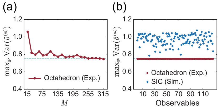
Figure 2: The results of experimental $\max_{\mathbf{P}}\text{Var}(\hat{o}^{(m)})$ with $\mathbf{E}_{\text{octa}}$ and simulated $\max_{\mathbf{P}}\text{Var}(\hat{o}^{(m)})$ with SIC POVM. (a), Experimental results of $\max_{\mathbf{P}}\text{Var}(\hat{o}^{(m)})$ for $O\in\mathbf{O}$ with different measurements $M$. (b), Experimental results of $\max_{\mathbf{P}}\text{Var}(\hat{o}^{(m)})$ with different observables $O$ (red dots). Simulated results of $\max_{\mathbf{P}}\text{Var}(\hat{o}^{(m)})$ with SIC POVM (blue diamonds). The 128 observables $\mathbf{O}$ are selected according to Haar random.

We first investigate the sample complexity by performing shadow tomography with $\mathbf{E}_{\text{octa}}$ on single-photon pure states $\rho=|\psi\rangle_{\gamma,\phi}\langle\psi|\in\mathbf{P}$ to estimate the expected value of observable in form of single-qubit projection $O\in\mathbf{O}$. As shown in Figure 1(e), the polarization-entangled photons (central wavelength of 810 nm) are generated from a periodically poled potassium titanyl phosphate (PPKTP) crystal placed in a Sagnac interferometer via spontaneous parametric down conversion (SPDC), which is pumped by a laser diode (central wavelength of 405 nm). The generated entangled photons are with ideal form of $|\psi\rangle_{\eta}=\sqrt{\eta}|HV\rangle+\sqrt{1-\eta}|VH\rangle$, where $\eta$ is determined by polarization of pump light. Projecting one photon of $|\psi\rangle_{\eta}$ on $|H\rangle$ heralds the other photon on state $|V\rangle$, which can further be transformed to arbitrary $|\psi\rangle_{\gamma,\phi}=\cos\gamma|H\rangle+\sin\gamma\text{e}^{i\phi}|V\rangle$ by a combination of electrically-rotated half-wave plate (E-HWP) and quarter-wave plate (E-QWP). Then, the heralded photon passes through the metasurface, and is coupled to six multimode fibers at outputs using an objective lens (OL), a tube lens, and three prisms, respectively. With the collection of classical shadows $\{\hat{\rho}^{(m)}\}_{m=1}^{M}$, the estimation of expected value of observable is $\hat{O}=1/M\sum_{m=1}^{M}\hat{o}^{(m)}$, where $\hat{o}^{(m)}={\rm Tr}(O\hat{\rho}^{(m)})$ is the i.i.d single-shot estimator. Note that $\hat{O}$ converges to the exact expectation value ${\rm Tr}(\rho O)$ as $M\to\infty$. The sample complexity of estimation is characterized by the variance $\text{Var}(\hat{O})=M^{-1}\text{Var}(\hat{o}^{(m)})\leq M^{-1}||O||^{2}_{\text{shd}}$. Here the shadow norm $||O||^{2}_{\text{shd}}$  Huang et al. (2020) is the maximization of $\text{Var}(\hat{o}^{(m)})$ over all possible states $\rho$ to remove the state-dependence. For ideal $\mathbf{E}_{\text{octa}}$, the shadow norm $||O||^{2}_{\text{shd}}=0.75$ regardless of the explicit form of the pure state vector $O\in\mathbf{O}$ Nguyen et al. (2022). To observe the varaince and the shadow norm in experiment, we use

$$\frac{1}{M}\sum_{m=1}^{M}\left(\hat{o}^{(m)}-\hat{O}\right)^{2},$$ (2)

to estimate the variance $\text{Var}(\hat{o}^{(m)})$, and prepare totally 20 $|\psi\rangle_{\gamma,\phi}$ forming the state set $\mathbf{P}$ that are uniformly distributed on Bloch sphere. For each $|\psi\rangle_{\gamma,\phi}$, we perform shadow tomography and the results of $\max_{\mathbf{P}}\text{Var}(\hat{o}^{(m)})$ are shown in Figure 2(a). We observe that $\max_{\mathbf{P}}\text{Var}(\hat{o}^{(m)})$ converges to 0.75 when $M>255$. In Figure 2(b), we show $\max_{\mathbf{P}}\text{Var}(\hat{o}^{(m)})$ of 128 observables $O\in\mathbf{O}$ with $M=315$ measurements, which agrees well with the theoretical prediction of $||O||^{2}_{\text{shd}}=0.75$. To give a comparison, we simulate $\max_{\mathbf{P}}\text{Var}(\hat{o}^{(m)})$ with symmetric informationally complete (SIC) POVM Renes et al. (2004), and the results are shown with blue diamonds in Figure 2(b). It is obvious that shadow norm with SIC POVM depends on observable $O$, and generally larger than that with $\mathbf{E}_{\text{octa}}$, which indicates $\mathbf{E}_{\text{octa}}$ outperforms SIC POVM in term of sample complexity in the estimation.

We then focus on the reconstruction of underlying state $\rho$ with shadow tomography. The direct estimation from classical shadows $\hat{\rho}^{(m)}$, i.e., $\hat{\rho}=1/M\sum_{m=1}^{M}\hat{\rho}^{(m)}$, is generally not a physical state with finite $M$ measurements, which limits the application of shadow tomography in estimation of nonlinear functions Stricker et al. (2022); Zhou and Liu (2022). Nonlinear functions Brydges et al. (2019); Elben et al. (2020a); Garcia et al. (2021); Liu et al. (2022), such as the purity and PT-moments, are of particular interest in detecting multipartite entanglement  Elben et al. (2020b); Zhou et al. (2020); Neven et al. (2021); Zhang et al. (2021), which is helpful in benchmarking the technologies towards generation of genuine multipartite entanglement Lu et al. (2018); Zhou et al. (2019, 2022). Physical constraints need to be introduced to enforce the positivity of the reconstructed state $\tau$, which can be addressed by the solving the optimization problem

$$\begin{split}\text{maximize}\hskip 34.14322pt&F(\hat{\rho},\tau)={\rm Tr}\left(\sqrt{\sqrt{\tau}\hat{\rho}\sqrt{\tau}}\right)\\ \text{subject to}\hskip 34.14322pt&\tau\geq 0,\hskip 2.0pt{\rm Tr}(\tau)=1,\end{split}$$ (3)

where $\tau$ is the proposed state that is positive semidefinite ($\tau\geq 0$) with unit trace (${\rm Tr}(\tau)=1$), and the loss function is the state fidelity $F(\hat{\rho},\tau)$ Ferrie (2014); Chapman et al. (2016); Rambach et al. (2021). We employ an iterative self-learning algorithm, i.e., SPSA algorithm Spall (1992), to solve the optimization problem in Eq. 3. Accordingly, the optimization is so-called self-learning shadow tomography (SLST).

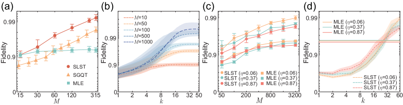
Figure 3: Experimental results of SLST on one-photon and two-photon states. (a), The average fidelity between reconstructed single-photon states $\tau_{k}$ and $|\psi\rangle_{\gamma,\phi}$ using three different techniques, i.e., SLST, SGQT, MLE tomography. (b), Average fidelity of SLST by increasing measurements $M$ from 10 to 1000. (c), Fidelity between reconstructed two-photon states $\tau_{k}$ and $\rho_{\eta}$ with SLST and MLE. (d), The fidelities of two-photon states reconstruction from SLST (dash lines) with $M=2000$ measurements. The solid lines represent the fidelity from MLE tomography with $M=2000$ measurements.

Generally, an $N$-qubit state $\tau$ can be modeled with $d^{2}$ parameters with $d=2^{N}$ the dimension of $\tau$. Thus, the proposed state $\tau$ is determined by a $d^{2}$-dimensional vector $\bm{r}=[r_{1},r_{2},\cdots,r_{d^{2}}]$. According, state fidelity is denoted by $F(\bm{r})=F(\hat{\rho},\tau)$. SPSA optimization estimates the gradient by simultaneously perturbing all parameters $r_{i}$ in a random direction, instead of individually addressing each $r_{i}$. In $k$-th iteration, the simultaneous perturbation approximation has all elements of $\bm{r}_{k}$ perturbed together by a random perturbation vector $\bm{\Delta}_{k}=[\Delta_{k1},\Delta_{k2},\cdots,\Delta_{kd^{2}}]$ with $\Delta_{ki}$ being generated from Bernoulli $\pm 1$ distribution with equal probability. Then the gradient is calculated by

$$\bm{g}_{k}=\frac{F(\bm{r}_{k}+\beta_{k}\bm{\Delta}_{k})-F(\bm{r}_{k}-\beta_{k}\bm{\Delta}_{k})}{2\beta_{k}}\bm{\Delta}_{k},$$ (4)

and $\bm{r}_{k}$ is updated to $\bm{r}_{k+1}$ by $\bm{r}_{k+1}=\bm{r}_{k}+\alpha_{k}\bm{g}_{k}$. $A_{k}$ and $B_{k}$ are functions in forms of $A_{k}={a_{1}}/{(k+a_{2})^{a_{3}}}$ and $B_{k}={b_{1}}/{k^{b_{2}}}$ with $a_{1}$, $a_{2}$, $a_{3}$, $b_{1}$ and $b_{2}$ being hyperparameters that determines the convergence speed of algorithm, which can be generally obtained from numerical simulations (see Supplementary Materials for hyperparameter settings). We terminate the algorithm if there is little change of $F(\bm{r}_{k})$ in several successive iterations, and corresponding $\tau_{k}$ is the reconstructed state.

The prepared single-photon state is with high fidelity with the ideal state $|\psi\rangle_{\gamma,\phi}$ so that we restrict the proposed state $\tau$ to be pure state, and use the fidelity between $\tau_{k}$ and target state $|\psi\rangle_{\gamma,\phi}$ to indicate the accuracy of reconstruction. The results of average fidelity of SLST over 20 prepared $|\psi\rangle_{\gamma,\phi}$ after $k=30$ iterations are shown with red dots in Figure 3(a). The average fidelity increases as $M$ increases, and achieves 0.992$\pm$0.001 with $M=315$ measurements. To give a comparison, we also demonstrate SGQT Ferrie (2014); Chapman et al. (2016); Rambach et al. (2021), in which 7 measurements are performed in each iteration. After 45 iterations (total number of 315 measurements), average fidelity reaches 0.983$\pm$0.003 as shown with yellow triangles in Figure 3(a). Moreover, we perform maximum likelihood estimation (MLE)  James et al. (2001b) on the prepared states as shown with cyan squares in Figure 3(a). When $M$ is small ($M<60$), MLE exhibits better accuracy than SGQT. However, SLST always exhibits advantage compared to other techniques in presence of experimental noises. Note that the fidelity does not keep increasing with the number of iterations as reflected in Figure 3(b). The fidelity is converged to a certain value depending on the number of measurements $M$ in classical shadow collection.

We also demonstrate SLST on two-photon entangled states $|\psi\rangle_{\eta}$ with $\eta=0.06,0.37$ and $0.87$. One photon is detected by metasurface-enabled $\mathbf{E}_{\text{octa}}$, and the other photon is detected by randomly choosing $\sigma_{x}$, $\sigma_{y}$ and $\sigma_{z}$ measurements that is realized by E-HWP and E-QWP. In contrast to high fidelity of single-photon state, the generated two-photon state $\rho_{\eta}$ is affected by more noises that are mainly attributed to high-order emission in SPDC and mode mismatch when overlapping two photons in Sagnac interferometer. Thus we decompose the proposed state $\tau_{k}$ in general form of $\tau_{k}=T^{\dagger}T$ with $T$ being a complex lower triangular matrix (see Supplementary Materials for more details). To benchmark the accuracy of reconstruction, we perform MLE on the prepared state $\rho_{\eta}$ with large number of measurements ($M\approx 8\times 10^{5}$), and the accuracy of SLST is indicated by the fidelity to MLE with large $M$. The results of $F(\tau_{60},\rho_{\eta})$ are shown with dots in Figure 3(c), the fidelities of three states reaches 0.986$\pm$0.002, 0.990$\pm$0.001 and 0.981$\pm$0.002 with $M=2000$ measurements and $k=60$ iterations. The MLE with same $M$ measurements are shown with squares in Figure 3(c). Again, two-photon SLST exhibits advantage compared to MLE. In Figure 3(d), we show that the accuracy of SLST beyond MLE with $M=2000$ measurements and iteration $k>20$ for all three states.

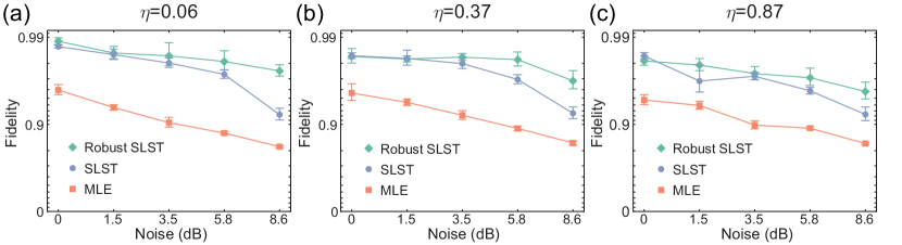
Figure 4: Results of fidelities from robust SLST, SLST and MLE tomography on two-photon states (a), $\rho_{\eta=0.06}$, (b), $\rho_{\eta=0.37}$ and (c), $\rho_{\eta=0.87}$. In three approaches, $M=1000$ measurements are used for reconstruction. In robust SLST, additional $M^{\prime}=2000$ measurements are used for calibration. We set $k=60$ in robust SLST and SLST.

Finally, we demonstrate the experimental noise can be further eliminated using robust classical shadow tomography Chen et al. (2021); Koh and Grewal (2022). To this end, the system is calibrated prior to the reconstruction of underlying state $\rho_{\eta}$. $M^{\prime}$ measurements is performed on high-fidelity state $|HH\rangle$ to calculate the noisy quantum channel $\mathcal{M}_{\text{R}}$, and accordingly the estimator is $\hat{\rho}^{(m)}=\mathcal{M}_{\text{R}}^{-1}(|\psi_{l_{1}}\rangle\langle\psi_{l_{1}}|\otimes|\psi_{l_{2}}\rangle\langle\psi_{l_{2}}|)$. We insert a tunable attenuator before metasurface to introduce optical loss noise from 1.5dB to 8.6dB, which reduces the signal-to-noise ratio from 3.7 to 0.7 accordingly. As shown in Figure 4, the fidelity of MLE decreases as optical loss increases due to the lower signal-to-noise ratio. The advantage of SLST is evident in the presence of noise, especially at the high-level optical loss, which returns the reconstructed state with fidelity higher than 0.985. This advantage is mainly attributed to the SPSA optimization.

In conclusion, we propose and demonstrate POVM with a single metasurface that enables implementation of real-time shadow tomography and observation of sample complexity. Together with the developed algorithms, the underlying quantum states can be reconstructed efficiently, accurately, and robustly, and the advantages are evident even in single- and two-photon experiment. Remarkable progresses highlight the scalability to generate large-scale multiphoton entanglement with the assistance of photon-atom interface Thomas et al. (2022); Yang et al. (2022) and multiplexing technologies Kaneda and Kwiat (2019); Meyer-Scott et al. (2022). As all the optical elements can be in principle replaced by metasurface, we can expect metasurface-based optical chip for large-scale multiphoton entanglement generation in the near further. Our results provide a compatible way for efficient characterization of multiphoton entanglement and empower the quantum information processing with ultra-thin quantum photonics .

Appendix A Shadow tomography with POVM

A.1 Constructing classical shadow with POVM

Consider a $d$-level quantum system, a set of $L$ rank-one projectors $\{|\psi_{l}\rangle\langle\psi_{l}|\in\mathbb{H}_{d}\}_{l=1}^{L}$ is called a quantum (complex projective) 2-design if the average value of second moment $(|\psi_{l}\rangle\langle\psi_{l}|)^{\otimes 2}$ over the set $\{|\psi_{l}\rangle\}$ is proportional to the symmetric subspace of two copies

$$\frac{1}{L}\sum_{l=1}^{L}(|\psi_{l}\rangle\langle\psi_{l}|)^{\otimes 2}=\binom{d+1}{2}^{-1}P_{\text{Sym}^{(2)}},$$ (5)

where $P_{\text{Sym}^{(2)}}=\frac{1}{2}(\mathds{1}_{d}\otimes\mathds{1}_{d}+\mathbb{F})$ is the projector of the symmetric subspace, and $\mathbb{F}$ is the swap operator acting on 2-copy as $\mathbb{F}|v\rangle\otimes|w\rangle=|w\rangle\otimes|v\rangle$ for all $|v\rangle,|w\rangle\in\mathbb{C}^{d}$.

Following the defining property Eq. 5, each quantum 2-design is proportional to a POVM

$$\mathbf{E}=\{E_{l}=\frac{d}{L}|\psi_{l}\rangle\langle\psi_{l}|\}_{l=1}^{L}$$ (6)

since the elements $E_{l}$ are positive semidefinite and satisfy $\sum_{l=1}^{L}E_{l}=\mathds{1}_{d}$. Measuring a quantum state $\rho$ results one of the $L$ outcomes indexed by $l\in[L]$, and by Born’s rule, the corresponding probability

$$p_{l}={\rm Pr}(l|\rho)={\rm Tr}(E_{l}\rho).$$ (7)

Hereafter we focus on the case of $d=2$. The POVM defined in Eq. 6 (together with the preparation of the corresponding state $|\psi_{l}\rangle$) can be viewed as a linear map $\mathcal{M}:\mathbb{H}_{2}\to\mathbb{H}_{2}$ as follows.

$$\begin{split}\mathcal{M}(\rho)&=\sum_{l=1}^{L}{\rm Pr}(l|\rho)|\psi_{l}\rangle\langle\psi_{l}|\\ &=\frac{2}{L}\sum_{l=1}^{L}\langle\psi_{l}|\rho|\psi_{l}\rangle|\psi_{l}\rangle\langle\psi_{l}|\\ &=\frac{2}{L}{\rm Tr}_{1}\left(\left(\sum_{l=1}^{L}(|\psi_{l}\rangle\langle\psi_{l}|)^{\otimes 2}\right)\mathds{1}_{2}\otimes\rho\right)\\ &=2{\rm Tr}_{1}\left(\frac{1}{6}(\mathds{1}_{2}\otimes\mathds{1}_{2}+\mathbb{F})\mathds{1}_{2}\otimes\rho\right)\\ &=\frac{1}{3}{\rm Tr}_{1}\left(\mathds{1}_{2}\otimes\rho+\rho\otimes\mathds{1}_{2}\right)\\ &=\frac{1}{3}\left(\rho+{\rm Tr}(\rho)\mathds{1}_{2}\right),\end{split}$$ (8)

where the forth line is by the property of 2-design in Eq. (5). The inverse of this map is

$$\mathcal{M}^{-1}(X)=3X-{\rm Tr}(X)\mathds{1}_{2}\ \forall X\in\mathbb{H}_{2}.$$ (9)

For single experimental run by performing POVM on $\rho$, we obtain the random outcome $l$ with probability ${\rm Pr}(l|\rho)$, and the classical shadow in constructed according to Eq. 9 as

$$\hat{\rho_{l}}=\mathcal{M}^{-1}(|\psi_{l}\rangle\langle\psi_{l}|)=3|\psi_{l}\rangle\langle\psi_{l}|-\mathds{1}_{2}.$$ (10)

It exactly reconstruct underlying quantum state $\rho$ in expectation

$$\begin{split}\mathbb{E}(\hat{\rho_{l}})&=\sum_{l}{\rm Pr}(l|\rho)(3|\psi_{l}\rangle\langle\psi_{l}|-\mathds{1}_{2})\\ &=3\sum_{l}{\rm Pr}(l|\rho)|\psi_{l}\rangle\langle\psi_{l}|-\mathds{1}_{2}\\ &=\rho+\mathds{1}_{2}-\mathds{1}_{2}\\ &=\rho,\end{split}$$ (11)

where the third line is due to Eq. (8).

For an $N$-qubit state $\rho\in\mathbb{H}_{2}^{\otimes N}$, the POVM $\mathbf{E}^{\otimes N}$ acts on each qubit independently yields outcome as a string $\bm{l}=l_{1}l_{2}\cdots l_{N}$ with probability

$$\begin{split}{\rm Pr}(\bm{l}|\rho)&={\rm Tr}\left(\rho\bigotimes_{n=1}^{N}E_{l_{n}}\right)\\ &=\left(\frac{2}{L}\right)^{N}\langle\psi_{\bm{l}}|\rho|\psi_{\bm{l}}\rangle,\end{split}$$ (12)

where $|\psi_{\bm{l}}\rangle=|\psi_{l_{1}}\rangle\otimes|\psi_{l_{2}}\rangle\otimes\cdots\otimes|\psi_{l_{N}}\rangle$. For a single experimental run, the classical shadow shows

$$\begin{split}\hat{\rho}&=\bigotimes_{n=1}^{N}\mathcal{M}^{-1}(|\psi_{\bm{l}}\rangle\langle\psi_{\bm{l}}|)\\ &=\bigotimes_{n=1}^{N}\mathcal{M}^{-1}(|\psi_{l_{n}}\rangle\langle\psi_{l_{n}}|)\\ &=\bigotimes_{n=1}^{N}\left(3|\psi_{l_{n}}\rangle\langle\psi_{l_{n}}|-\mathds{1}_{2}\right)\end{split}$$ (13)

which is in a tensor-product form.

A.2 Calibration of quantum channel $\mathcal{M}$

In practice, there are unavoidable noise in unitary operations and measurements. To address this issue, robust classical shadow (RShadow) protocol was proposed to mitigate the noise in shadow tomography Chen et al. (2021). It is convenient to represent $\mathcal{M}$ as a matrix $\mathcal{L}_{\mathcal{M}}$ in Pauli-Liouville representation. Here a linear operator $X$ is represented by a column vector $|X\rangle\!\rangle_{j}={\rm Tr}(\sigma_{j}X)$ in the Pauli-basis with $\sigma_{0}=\mathds{1}_{2}/\sqrt{2}$ and $\sigma_{1}$, $\sigma_{2}$, $\sigma_{3}$ being the Pauli matrix $X/\sqrt{2}$, $Y/\sqrt{2}$, $Z/\sqrt{2}$. In this way Eq. 8 can be expressed as

$$\begin{split}\mathcal{L}_{\mathcal{M}}|\rho\rangle\!\rangle&=\sum_{l}\langle\!\langle E_{l}|\rho\rangle\!\rangle|\psi_{l}\rangle\!\rangle\\ &=\frac{2}{L}\sum_{l}|\psi_{l}\rangle\!\rangle\langle\!\langle\psi_{l}||\rho\rangle\!\rangle.\end{split}$$ (14)

The matrix form $\mathcal{L}_{\mathcal{M}}$ of the channel $\mathcal{M}$ corresponds to the projector onto the subspace spanned by $\mathbf{E}$, which is given by

$$\mathcal{L}_{\mathcal{M}}=\frac{2}{L}\sum_{l=1}^{L}|\psi_{l}\rangle\!\rangle\langle\!\langle\psi_{l}|,$$ (15)

and the classical shadow is

$$|\hat{\rho}\rangle\!\rangle=\mathcal{L}_{\mathcal{M}}^{-1}|\psi_{l}\rangle\!\rangle,$$ (16)

where $\mathcal{L}_{\mathcal{M}}^{-1}$ is the Moore-Penrose pseudo inverse of $\mathcal{L}_{\mathcal{M}}$ Penrose (1956).

The POVM $\mathbf{E}_{\text{octa}}=\{\frac{1}{3}|\psi_{l}\rangle\langle\psi_{l}|:l=1,\cdots,6\}$ with corresponding normalized vector $|\psi_{l}\rangle\in\{|0\rangle,|1\rangle,|+\rangle,|-\rangle,|R\rangle,|L\rangle\}$. The matrix $\mathcal{L}_{\mathcal{M}}$ and its inverse $\mathcal{L}_{\mathcal{M}}^{-1}$ are

$$\mathcal{L}_{\mathcal{M}}=\begin{pmatrix}1&0&0&0\\ 0&\frac{1}{3}&0&0\\ 0&0&\frac{1}{3}&0\\ 0&0&0&\frac{1}{3}\end{pmatrix},\ \ \mathcal{L}_{\mathcal{M}}^{-1}=\begin{pmatrix}1&0&0&0\\ 0&3&0&0\\ 0&0&3&0\\ 0&0&0&3\end{pmatrix}.$$ (17)

Accordingly, one has

$$\mathcal{L}_{\mathcal{M}}|\rho\rangle\!\rangle=\frac{1}{3}(|\rho\rangle\!\rangle+|\mathds{1}_{2}\rangle\!\rangle),$$ (18)

which is a depolarizing channel. Accordingly, the classical shadow in Eq. 10 can be written as

$$\begin{split}|\hat{\rho}\rangle\!\rangle&=\mathcal{L}_{\mathcal{M}}^{-1}|\psi_{l}\rangle\!\rangle=3|\psi_{l}\rangle\!\rangle-|\mathds{1}_{2}\rangle\!\rangle\Leftrightarrow\hat{\rho}=3|\psi_{l}\rangle\langle\psi_{l}|-\mathds{1}_{2}\end{split}$$ (19)

Similarly, for an N-qubit state $\rho$,

$$\begin{split}\mathcal{L}_{\mathcal{M}}|\rho\rangle\!\rangle&=\sum_{\bm{l}}{\rm Pr}(\bm{l}|\rho)|\psi_{\bm{l}}\rangle\!\rangle\\ &=\sum_{l_{1},l_{2},\cdots,l_{N}}\langle\!\langle\bigotimes_{n=1}^{N}E_{l_{n}}|\rho\rangle\!\rangle|\bigotimes_{n=1}^{N}\psi_{l_{n}}\rangle\!\rangle\\ &=\bigotimes_{n=1}^{N}\left[\frac{1}{3}\sum_{l_{n}}|\psi_{l_{n}}\rangle\!\rangle\langle\!\langle\psi_{l_{n}}|\right]|\rho\rangle\!\rangle\\ &=\bigotimes_{n=1}^{N}\mathcal{L}_{\mathcal{M}_{n}}|\rho\rangle\!\rangle.\end{split}$$ (20)

Then we have

$$\mathcal{L}_{\mathcal{M}}=\bigotimes_{n=1}^{N}\mathcal{L}_{\mathcal{M}_{n}},$$ (21)

and the classical shadow is

$$\begin{split}|\hat{\rho}\rangle\!\rangle&=\mathcal{L}_{\mathcal{M}}^{-1}\bigotimes_{n=1}^{N}|\psi_{l_{n}}\rangle\!\rangle\\ &=\bigotimes_{n=1}^{N}\mathcal{L}_{\mathcal{M}_{n}}^{-1}|\psi_{l_{n}}\rangle\!\rangle\\ &=\bigotimes_{n=1}^{N}(3|\psi_{l_{n}}\rangle\!\rangle-|\mathds{1}_{2}\rangle\!\rangle).\end{split}$$ (22)

The quantum channel in Eq. 21 can be written as

$$\mathcal{L}_{\mathcal{M}}=\sum_{\lambda\in\{0,1\}^{N}}f_{\lambda}\Pi_{\lambda}$$ (23)

where $\lambda$ is an $n$-bit vector denoting the subspaces due to the irreducible representation, and $\Pi_{\lambda}=\bigotimes_{n=1}^{N}\Pi_{\lambda_{n}}$ in the tensor-product form with

$$\Pi_{\lambda_{n}}=\begin{cases}|\sigma_{0}\rangle\!\rangle\langle\!\langle\sigma_{0}|,&\lambda_{n}=0\\ \mathds{1}_{4}-|\sigma_{0}\rangle\!\rangle\langle\!\langle\sigma_{0}|,&\lambda_{n}=1.\end{cases}$$ (24)

Here $\sigma_{0}=\mathds{1}_{2}/\sqrt{2}$ is the normalized single-qubit identity operator such that $\langle\!\langle\sigma_{0}|\sigma_{0}\rangle\!\rangle=1$, and $\mathds{1}_{4}$ is the 4-dimentional idenity matrix for this single-qubit operator space. That is, $\Pi_{0}$ subsapce corresponds to the identity operartor, and $\Pi_{1}$ is the complementary subspace spanned by the Pauli operators evenly. In the noiseless case,

$$f_{\lambda}=\frac{1}{3^{|{\lambda}|}}.$$ (25)

where $|{\lambda}|$ is the number of $1$s in the $n$-bit vector $\lambda$. For the single-qubit case with $N=1$, the matrix form of $\mathcal{L}_{\mathcal{M}}$ is just shown in Eq. (17).

Considering the noise (or imperfections) in practice, suppose the corresponding quantum channel of the noisy POVM (noisy measurement or perfect perparation) can be written as $\mathcal{L}_{\widetilde{\mathcal{M}}}=\sum_{\lambda}\tilde{f}_{\lambda}\Pi_{\lambda}$, which is still diagonal according to the subspaces. The noisy parameters $\tilde{f}_{\lambda}$ can be experimentally calibrated.

To this end, a high-fidelity $N$-qubit product state

$$\rho_{\mathbf{0}}=\bigotimes_{n=1}^{N}|0\rangle\langle 0|\Leftrightarrow|\rho_{\mathbf{0}}\rangle\!\rangle=\bigotimes_{n=1}^{N}\frac{1}{2}(|\mathds{1}_{2}\rangle\!\rangle+|Z\rangle\!\rangle)$$ (26)

is prepared and measured with noisy POVM, and the probability is $\tilde{{\rm Pr}}({\bm{l}})=\langle\!\langle\tilde{E}_{\bm{l}}|\rho_{\mathbf{0}}\rangle\!\rangle$ with $|\tilde{E}_{\bm{l}}\rangle\!\rangle$ being the noisy POVM.

Here we define $|P_{\lambda}\rangle\!\rangle=\bigotimes_{n=1}^{N}|Z^{\lambda_{n}}\rangle\!\rangle$, we can use $\langle\!\langle P_{\lambda}|\psi_{\bm{l}}\rangle\!\rangle$ to estimate the noisy parameter $\tilde{f}_{\lambda}$. To show this is indeed an unbiased estimator, we take the expectation value and find that

$$\begin{split}\mathbb{E}\langle\!\langle P_{\lambda}|\psi_{\bm{l}}\rangle\!\rangle=&\sum_{\bm{l}}\langle\!\langle P_{\lambda}|\psi_{\bm{l}}\rangle\!\rangle\langle\!\langle\tilde{E}_{\bm{l}}|\rho_{\mathbf{0}}\rangle\!\rangle\\ =&\langle\!\langle P_{\lambda}|\mathcal{L}_{\widetilde{\mathcal{M}}}|\rho_{\mathbf{0}}\rangle\!\rangle\\ =&\frac{1}{2^{N}}\left(\bigotimes_{n=1}^{N}\langle\!\langle Z^{\lambda_{n}}|\right)\sum_{\lambda^{\prime}}\tilde{f}_{\lambda^{\prime}}\Pi_{\lambda^{\prime}}\bigotimes_{n=1}^{N}(|\mathds{1}_{2}\rangle\!\rangle+|Z\rangle\!\rangle)\\ =&\frac{1}{2^{N}}\left(\bigotimes_{n=1}^{N}\langle\!\langle Z^{\lambda_{n}}|\right)\sum_{\lambda^{\prime}}\tilde{f}_{\lambda^{\prime}}\bigotimes_{n=1}^{N}|Z^{\lambda^{\prime}_{n}}\rangle\!\rangle=\tilde{f}_{\lambda}.\end{split}$$ (27)

In real experiment, we just record the result $\bm{l}$ from the noisy POVM, and then calculate the value $\langle\!\langle P_{\lambda}|\psi_{\bm{l}}\rangle\!\rangle$ on the classical computer which serves an estimation of $\tilde{f}_{\lambda}$. One can repeat this process say $M$ times, and average them to make the estimation more accurate.

In this way, we can get the noisy parameters $\tilde{f}_{\lambda}$ of the noisy channel $\widetilde{\mathcal{M}}$, and the matrix form of its inverse $\widetilde{\mathcal{M}}^{-1}$ is just

$$\mathcal{L}_{\mathcal{M}}^{-1}=\sum_{\lambda\in\{0,1\}^{N}}\tilde{f}^{-1}_{\lambda}\Pi_{\lambda}$$ (28)

In post-processing, we can use this new inverse channel instead of the original one, such that the error in the noisy POVM could be mitigated.

A.3 Simulation of shadow norm with SIC POVM

For a given $O$ and given state $\rho$, in practice we conduct $M$ rounds of experiments and use the following quantity to estimate the variance,

$$\frac{1}{M}\sum_{m=1}^{M}\left(\hat{o}^{(m)}-\hat{O}\right)^{2},$$ (29)

where $\hat{o}^{(m)}={\rm Tr}(O\hat{\rho}^{(m)})$ is the $m$-th i.i.d single-shot estimator, and $\hat{O}=1/M\sum_{m=1}^{M}\hat{o}^{(m)}$. When $M\to\infty$, the variance of estimating an observable $O\in\mathbf{O}$ with POVM $\mathbf{E}$ shows

$$\begin{split}\text{Var}(\hat{O})&=\sum_{l=1}^{L}{\rm Tr}(\hat{\rho}_{l}O)^{2}{\rm Tr}(\rho E_{l})-{\rm Tr}(\rho O)^{2}\\ &\leq\max_{\rho\in\mathbf{P}}\sum_{l=1}^{L}{\rm Tr}(\hat{\rho}_{l}O)^{2}{\rm Tr}(\rho E_{l})-{\rm Tr}(\rho O)^{2}\doteq||O||^{2}_{\text{shd}},\end{split}$$ (30)

where $\rho$ is the underlying state, and $\hat{\rho}_{l}=3|\psi_{l}\rangle\langle\psi_{l}|-\mathds{1}_{2}$ is the estimator. Being the upper bound of $\text{Var}(\hat{O})$, the shadow norm $||O||^{2}_{\text{shd}}$ is obtained by maximizing the first term over all possible states $\rho\in\mathbf{P}$. To calculate the shadow norm with SIC POVM, we consider 128 observables $O\in\mathbf{O}$ and 20 states $\rho=|\psi\rangle_{\gamma,\phi}\langle\psi|$ forming the state set $\mathbf{P}$.

For single-qubit system, the SIC POVM is 2-design and can be expressed as $\mathbf{E}_{\text{SIC}}=\{\frac{1}{2}|\psi_{l}\rangle\langle\psi_{l}|\}_{l=1}^{4}$ with

$$\left|\psi_{1}\right\rangle=|0\rangle$$ (31)

$$\left|\psi_{2}\right\rangle=\frac{1}{\sqrt{3}}|0\rangle+\sqrt{\frac{2}{3}}|1\rangle$$

$$\left|\psi_{3}\right\rangle=\frac{1}{\sqrt{3}}|0\rangle+\sqrt{\frac{2}{3}}e^{i\frac{2\pi}{3}}|1\rangle$$

$$\left|\psi_{4}\right\rangle=\frac{1}{\sqrt{3}}|0\rangle+\sqrt{\frac{2}{3}}e^{i\frac{4\pi}{3}}|1\rangle.$$

Appendix B Details of SLST

B.1 Setting of hyperparameters in SPSA optimization

The setting of hyperparameters $a_{1}$, $a_{2}$, $a_{3}$, $b_{1}$ and $b_{2}$ determines the convergence of SPSA optimization. Previous investigations have concluded that $a_{3}=0.602,b_{2}=0.101$ are generally good choices for most optimization tasks Spall (1992, 1998); Maryak and Chin (2001), so that we set $a_{3}=0.602,b_{2}=0.101$ in our optimization. Besides, we find that $a_{2}$ is trivial compared with other four hyperparameters so that we set $a_{2}=0$. $a_{1}$ and $b_{1}$ are determined through numerical simulations. We set $a_{1}=13$, $b_{1}=0.5$ in single-photon experiment, while $a_{1}=48$ and $b_{1}=1.1$ in two-photon experiment.

B.2 Model of proposed state $\tau_{k}$ in SLST

If the underlying quantum state is close to pure state, the proposed state $\tau_{k}$ can be modeled by a $N$-qubit pure state $\tau_{k}=|\zeta\rangle\langle\zeta|$ with dimension $d=2^{N}$

$$|\zeta\rangle=\frac{1}{\sqrt{\sum_{i=1}^{d}r_{i}^{2}}}\left(\begin{array}[]{cc}r_{1}\\ r_{2}e^{ir_{d+1}}\\ r_{3}e^{ir_{{d+2}}}\\ \vdots\\ r_{d}e^{ir_{2d-1}}\\ \end{array}\right).$$ (32)

We set $\bm{r}_{k}=\{r_{1},r_{2},\cdots,r_{2d-1}\}$ with $r_{i}\in\mathbb{R}$ in SPSA optimization.

For general case, a mixed state, the proposed state $\tau_{k}$ is modeled by Cholesky decomposition

$$\tau_{k}=\frac{TT^{\dagger}}{{\rm Tr}(TT^{\dagger})},$$ (33)

where $T$ is a lower triangular matrix

$$T=\begin{pmatrix}r_{1}&0&\cdots&0\\ r_{d+1}+ir_{d+2}&r_{2}&\cdots&0\\ \vdots&\vdots&\ddots&\vdots\\ r_{d^{2}-1}+ir_{d^{2}}&r_{d^{2}-3}+ir_{d^{2}-2}&\cdots&r_{d}\\ \end{pmatrix}.$$ (34)

We set $\bm{r}_{k}=\{r_{1},r_{2},\cdots,r_{d^{2}}\},r_{i}\in\mathbb{R}$ in SPSA optimization.

B.3 Scaling of SLST

To investigate the scaling of SLST, we simulate SLST with POVM $\mathbf{E}_{\text{octa}}$ on 50 randomly generated $N$-qubit pure states with $N=2,4,6$ and $8$, respectively. The results of infidelity $1-F(\tau_{k},\hat{\rho})$ are shown in Fig. 5, in which we set the iterations $k=200,1000,5000$ and $25000$ for $N=2$, $4$, $6$ and $8$, respectively. The extracted scaling of SLST is $O(d\log d/M)$, which is slightly worse than $O(d/M)$ of SQT and $O(d^{\eta}/M)(\eta>1)$ of SGQT. However, SLST with POVM requires only one experimental setting and the POVM is locally implemented on individual qubit, which are friendly to experiment. A comparison of these technologies is shown in Table 1.

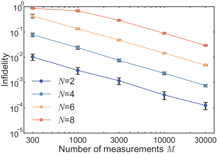
Figure 5: The average infidelity of 50 reconstructed states with number of measurements $M$. The error bars represent the deviation of estimation. The hyperparameters we set in SPSA optimization are $a_{1}=20,b_{1}=0.35$ for $N=2$, $a_{1}=15,b_{1}=0.79$ for $N=4$, $a_{1}=30,b_{1}=0.92$ for $N=6$ and $a_{1}=77,b_{1}=0.92$ for $N=8$.

	Infidelity	Experimental Setting	Measurement Type	Online/Offline
SQT	$O(d/M)$	$O(d)$	Global projective measurement	Offline
SGQT	$O(d^{\eta}/M)$	$O(M)$	Global projective measurement	Online
SLST with POVM	$O(d\log d/M)$	$1$	Local POVM	Online

Table 1: Comparison of SQT, SGQT and SLST with POVM.

Appendix C Initial setting of $\tau_{0}$

Generally, achieving the global minimum instead of local minimum is challenging in optimization. Indeed, SPSA optimization avoids local minimum under asymptotic iterations due to stochastic perturbation Maryak and Chin (2001). However, SPSA optimization does not guarantee the global convergence in each iteration Spall (1998); Maryak and Chin (2001). We show that the global convergence in each iteration can be improved by setting initial $\tau_{0}$ with prior information, instead of randomly setting initial $\tau_{0}$.

The direct estimation from classical shadows $\hat{\rho}=\frac{1}{M}\sum_{m=1}^{M}\hat{\rho}^{(m)}$ returns a Hermitian matrix, which has an eigen-decomposition in form of

$$\hat{\rho}=\sum_{i=1}^{d}\lambda_{i}|\Psi_{i}\rangle\langle\Psi_{i}|$$ (35)

with $\lambda_{i}$ and $|\Psi_{i}\rangle$ being the eigenvalue and eigenvector of $\hat{\rho}$. However, $\hat{\rho}$ is not a semi-positive matrix so that $\lambda_{i}$ might be negative. We set the initial $\tau_{0}$ as

$$\tau_{0}=\frac{\sum_{i=1}^{d}|\lambda_{i}||\Psi_{i}\rangle\langle\Psi_{i}|}{\sum_{i=1}^{d}|\lambda_{i}|},$$ (36)

which is close to $\hat{\rho}$. Then, we do Cholesky decomposition on $\tau_{0}$ according to Eq. 33, and obtain the corresponding $\bm{r}_{0}$ to start SPSA optimization.

To show the advantage of this modification, we simulate the SLST with $M=2000,3500$ and $5000$ measurements on randomly generated 2-, 3- and 4-qubit mixed states, respectively. The results are shown in Fig. 6. We observe that the initial setting of $\tau_{0}$ significantly influence efficiency and accuracy of SLST. With modified $\tau_{0}$, SLST converges more quickly and achieves lower infidelity than that with random setting of $\tau_{0}$.

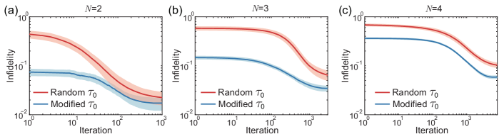
Figure 6: Simulation of SLST with different initial $\tau_{0}$. Blue line and red line represent the infidelity against iteration with modified $\tau_{0}$ and random $\tau_{0}$ of SLST on (a) $N=2$, (b) $N=3$ and (c) $N=4$ mixed states, respectively. The error bands represent the standard deviation of infidelities of 100 randomly generated mixed states. The hyperparameters we set in SPSA with modified $\tau_{0}$ are $a_{1}=8.5,b_{1}=1.4$ for $N=2$, $a_{1}=12.3,b_{1}=2.1$ for $N=3$ and $a_{1}=16.4,b_{1}=2.8$ for $N=4$. The hyperparameters we set in SPSA with random $\tau_{0}$ are $a_{1}=48,b_{1}=1.1$ for $N=2$, $a_{1}=44,b_{1}=8.0$ for $N=3$ and $a_{1}=49,b_{1}=12.7$ for $N=4$.

Appendix D Design, fabrication and characterization of metasurface

D.1 Design of metasurface to realize POVM $\mathbf{E}_{\text{octa}}$

The POVM $\mathbf{E}_{\text{octa}}$ is equivalent to randomly selecting three Pauli observables and then performing projective measurement on its eigenstates. To this end, the metasurface is designed to consist of three regions with same size ($210\mu m\times 70\mu m$), each of which corresponds to the projective measurement of observable $\sigma_{j},j\in\{x,y,z\}$. Each region is further designed to spatially separate eigenstates $|\psi_{\sigma_{j}}^{+}\rangle$ and $|\psi_{\sigma_{j}}^{-}\rangle$ of $\sigma_{j}$, which is achieved by individual phase control of $|\psi_{\sigma_{j}}^{+}\rangle$ and $|\psi_{\sigma_{j}}^{-}\rangle$ when they pass through metasurface by

$$\Phi_{\sigma_{j}}^{\pm}(x,y)=-\frac{2\pi}{\lambda}\left(\sqrt{(x-x_{\sigma_{j},0}^{\pm})^{2}+(y-y_{\sigma_{j},0}^{\pm})^{2}+f^{2}}-f\right).$$ (37)

$\Phi_{\sigma_{j}}^{\pm}(x,y)$ represents phase configuration at the output of metasurface with input polarization $|\psi_{\sigma_{j}}^{+}\rangle$ and $|\psi_{\sigma_{j}}^{-}\rangle$, $(x^{+}_{\sigma_{j},0},y^{+}_{\sigma_{j},0})$ and $(x^{-}_{\sigma_{j},0},y^{-}_{\sigma_{j},0})$ are the positions of separated focal spots of $|\psi_{\sigma_{j}}^{+}\rangle$ and $|\psi_{\sigma_{j}}^{-}\rangle$ at focal plane and $f$ is the focal length. Our aim is to design a metasurface to realize phase configuration of $\Phi_{j}^{\pm}(x,y)$ calculated according to Eq. 37 with fixed $(x^{\pm}_{\sigma_{j},0},y^{\pm}_{\sigma_{j},0})$, $\lambda$ and $f$. The parameters we set to calculate $\Phi_{\sigma_{j}}^{\pm}(x,y)$ are shown in Table 2.

Parameters	Values
$x$ in $\Phi_{\sigma_{x}}^{\pm}(x,y)$	$[-105\mu\text{m},105\mu\text{m}]$ with interval of 0.5$\mu\text{m}$
$y$ in $\Phi_{\sigma_{x}}^{\pm}(x,y)$	$[-35\mu\text{m},35\mu\text{m}]$ with interval of 0.5$\mu\text{m}$
$(x^{\pm}_{\sigma_{x},0},y^{\pm}_{\sigma_{x},0})$	$(\pm 35\mu\text{m},0\mu\text{m})$
$x$ in $\Phi_{\sigma_{y}}^{\pm}(x,y)$	$[-105\mu\text{m},105\mu\text{m}]$ with interval of 0.5$\mu\text{m}$
$y$ in $\Phi_{\sigma_{y}}^{\pm}(x,y)$	$[-105\mu\text{m},-35\mu\text{m}]$ with interval of 0.5$\mu\text{m}$
$(x^{\pm}_{\sigma_{y},0},y^{\pm}_{\sigma_{y},0})$	$(\pm 35\mu\text{m},-70\mu\text{m})$
$x$ in $\Phi_{\sigma_{z}}^{\pm}(x,y)$	$[-105\mu\text{m},105\mu\text{m}]$ with interval of 0.5$\mu\text{m}$
$y$ in $\Phi_{\sigma_{z}}^{\pm}(x,y)$	$[35\mu\text{m},105\mu\text{m}]$ with interval of 0.5$\mu\text{m}$
$(x^{\pm}_{\sigma_{z},0},y^{\pm}_{\sigma_{z},0})$	$(\pm 35\mu\text{m},70\mu\text{m})$
$f$	$150\mu\text{m}$
$\lambda$	$810\text{nm}$

Table 2: The values of parameters set in calculation of phase configurations $\Phi_{\sigma_{j}}^{\pm}(x,y)$ in Eq. 37.

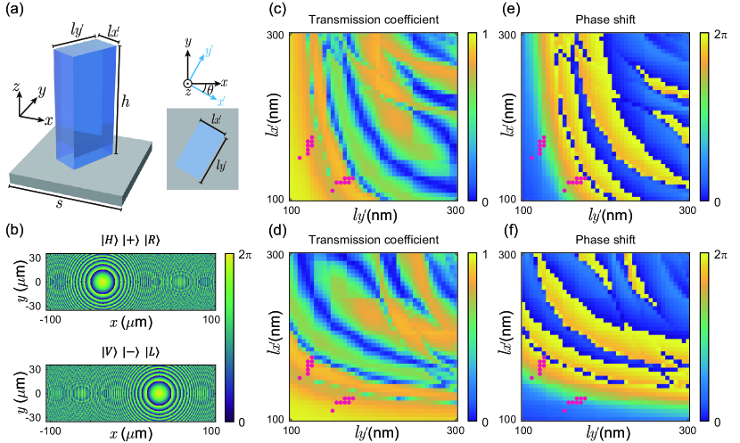
Figure 7: Schematic diagram and design of the metasurface. (a), Schematic of the designed meta-atom consisting of an a-Si nanopillar on a fused-silica substrate. (b), Target phase configuration for orthogonally polarized states when light pass through metasurface. (c) and (d), Mapping of transmission coefficient for linear polarizaiton along $x^{\prime}$ and $y^{\prime}$, respectively, as a function of the parameters $l_{x^{\prime}}$ and $l_{y^{\prime}}$ of the nanopillars. (e) and (f), Mapping of phase shift $\varphi_{x^{\prime}}$ and $\varphi_{y^{\prime}}$, as a function of the parameters $l_{x^{\prime}}$ and $l_{y^{\prime}}$ of the nanopillars.

The calculated phase configurations of $\Phi_{\sigma_{j}}^{+}(x,y)$ and $\Phi_{\sigma_{j}}^{-}(x,y)$ are shown in Fig. 7(b). To realize phase configurations $\Phi_{\sigma_{j}}^{\pm}(x,y)$, we design the metasurface consisting of $420\times 140$ nanopillars with interval of $500$nm. As shown in Fig. 7(a), the nanopillar located at position $(x_{i},y_{i})$ can be regarded as a polarization-dependent scatter acting on input polarization with transformation matrix

$$U_{\text{pillar}}=\begin{pmatrix}\cos\theta&-\sin\theta\\ \sin\theta&\cos\theta\\ \end{pmatrix}\begin{pmatrix}e^{i\varphi_{x^{\prime}}}&0\\ 0&e^{i\varphi_{y^{\prime}}}\\ \end{pmatrix}\begin{pmatrix}\cos\theta&\sin\theta\\ -\sin\theta&\cos\theta\\ \end{pmatrix}.$$ (38)

Here, $\theta$ is the angle of nanopillar, $\varphi_{x^{\prime}}$ and $\varphi_{y^{\prime}}$ are the phase accumulated on the polarization component decomposed along the direction $x^{\prime}$ and $y^{\prime}$ respectively, which are determined by length $l_{x^{\prime}}$ and $l_{y^{\prime}}$. Thus, by properly designing the parameters $\{\theta,l_{x^{\prime}},l_{y^{\prime}}\}$ of nanopillar at each $(x_{i},y_{i})$, we can realize the desired phase configuration $\Phi_{\sigma_{j}}^{+}(x,y)$ and $\Phi_{\sigma_{j}}^{-}(x,y)$ for polarization $|\psi_{\sigma_{j}}^{+}\rangle$ and $|\psi_{\sigma_{j}}^{-}\rangle$, respectively.

The numerical simulation results of $\varphi_{x^{\prime}}$ and $\varphi_{y^{\prime}}$ are shown in Fig. 7(e) and Fig. 7(f) respectively, in which we set $l_{x^{\prime}}$ and $l_{y^{\prime}}$ from $100$nm to $300$nm with interval of $5$nm. The corresponding transmittances are shown in Fig. 7(c) and Fig. 7(d) respectively. The choice of $\{\theta,l_{x^{\prime}},l_{y^{\prime}}\}$ depends on the polarization $|\psi_{\sigma_{j}}^{+}\rangle$ and $|\psi_{\sigma_{j}}^{-}\rangle$ we want to separate, and we will discuss separately.

D.1.1 Separation of linear polarizations

For linear polarizations $|\psi_{\sigma_{z}}^{\pm}\rangle$ and $|\psi_{\sigma_{x}}^{\pm}\rangle$, we set $\theta$ of all nanopillars to be a constant. In this sense, phase configuration is determined by phase $\varphi_{x^{\prime}}$ and $\varphi_{y^{\prime}}$ in Eq. 38. Specifically, to separate polarization $|H\rangle$ ($|\psi_{\sigma_{z}}^{+}\rangle$) and $|V\rangle$ ($|\psi_{\sigma_{z}}^{-}\rangle$), we set $\theta=0^{\circ}$ that leads to $x^{\prime}=x$ and $y^{\prime}=y$. According to Eq. 38, the transformation of $|H\rangle$ and $|V\rangle$ after a single nanopillar is

$$U_{\text{pillar}}|H\rangle=e^{i\varphi_{x^{\prime}}}|H\rangle,U_{\text{pillar}}|V\rangle=e^{i\varphi_{y^{\prime}}}|V\rangle.$$ (39)

According to the value of $\Phi_{\sigma_{z}}^{\pm}(x_{i},y_{i})$ at position $(x_{i},y_{i})$, we determine $l_{x^{\prime}}$ and $l_{y^{\prime}}$ by $\varphi_{x^{\prime}}\approx\Phi_{\sigma_{z}}^{+}(x_{i},y_{i})$ (Fig. 7(e)) and $\varphi_{y^{\prime}}\approx\Phi_{\sigma_{z}}^{-}(x_{i},y_{i})$ (Fig. 7(f)). Note that the choice of $(l_{x^{\prime}},l_{y^{\prime}})$ is not unique, and the transmittances with corresponding $(l_{x^{\prime}},l_{y^{\prime}})$ shown in Fig. 7(c) and Fig. 7(d) should be as high as possible.

To separate polarizations $|+\rangle$ ($|\psi_{\sigma_{x}}^{+}\rangle$) and $|-\rangle$ ($|\psi_{\sigma_{x}}^{-}\rangle$), we set $\theta=45^{\circ}$ for all nanopillars. According to Eq. 38, the transformation of a single nanopillar is

$$U_{\text{pillar}}|+\rangle=e^{i\varphi_{x^{\prime}}}|+\rangle,U_{\text{pillar}}|-\rangle=e^{i\varphi_{y^{\prime}}}|-\rangle.$$ (40)

Similar to the situation of $\Phi_{\sigma_{z}}^{\pm}(x_{i},y_{i})$, the value of $(l_{x^{\prime}},l_{y^{\prime}})$ is determined by $\varphi_{x^{\prime}}\approx\Phi_{\sigma_{x}}^{+}(x_{i},y_{i})$ and $\varphi_{y^{\prime}}\approx\Phi_{\sigma_{x}}^{-}(x_{i},y_{i})$ along with the consideration of high transmittance.

D.1.2 Separation of circular polarizations

The design to separate circular polarizations $|L\rangle$ ($|\psi_{\sigma_{y}}^{+}\rangle$) and $|R\rangle$ ($|\psi_{\sigma_{y}}^{-}\rangle$) is different with the situations of linear polarizations. To realize $\Phi_{\sigma_{y}}^{\pm}(x_{i},y_{i})$, $\varphi_{x^{\prime}}$ and $\varphi_{y^{\prime}}$ in Eq. 38 should satisfy $\lvert\varphi_{x^{\prime}}-\varphi_{y^{\prime}}\rvert=\pi$ Li et al. (2019). With this constraint, a single nanopillar transforms $|L\rangle$ and $|R\rangle$ by

$$U_{\text{pillar}}|L\rangle=e^{i(\varphi_{x^{\prime}}+2\theta)}|R\rangle,U_{\text{pillar}}|R\rangle=e^{i(\varphi_{x^{\prime}}-2\theta)}|L\rangle.$$ (41)

The values of $\theta$ and $\varphi_{x^{\prime}}$ are determined by

$$\left\{\begin{aligned} \theta=\frac{\Phi_{\sigma_{y}}^{+}(x_{i},y_{i})-\Phi_{\sigma_{y}}^{-}(x_{i},y_{i})}{4}\\ \varphi_{x^{\prime}}=\frac{\Phi_{\sigma_{y}}^{+}(x_{i},y_{i})+\Phi_{\sigma_{y}}^{-}(x_{i},y_{i})}{2}\\ \end{aligned}\right.$$ (42)

For the convince of fabrication, we choose nanopillars with 16 different $(l_{x^{\prime}},l_{y^{\prime}})$ shown with red dots in Fig. 7(c)-(f), and the parameters are shown in Table 3. For the phase $\Phi_{\sigma_{y}}^{\pm}(x_{i},y_{i})$ at position $(x_{i},y_{i})$, we calculate $\theta$ and $\varphi_{x^{\prime}}$ according to Eq. 42, and choose the closest $\varphi_{x^{\prime}}$ in Table 3 for fabrication.

$l_{x^{\prime}}\ (\text{nm})$	$l_{y^{\prime}}\ (\text{nm})$	$\varphi_{x^{\prime}}\ /\ 2\pi$	$\varphi_{y^{\prime}}\ /\ 2\pi$	$\mathbf{T}_{x^{\prime}}$	$\mathbf{T}_{y^{\prime}}$
110	150	0.1544	0.5924	0.9365	0.7640
120	155	0.2594	0.7413	0.8770	0.8245
120	160	0.2718	0.7972	0.8710	0.8567
120	165	0.2948	0.8546	0.8646	0.8837
120	170	0.3108	0.9024	0.8579	0.8803
125	165	0.4453	0.8751	0.8087	0.8857
125	170	0.4723	0.9251	0.8016	0.8618
125	175	0.4963	0.9698	0.7950	0.7676
150	110	0.5924	0.1544	0.7640	0.9365
155	120	0.7413	0.2594	0.8245	0.8770
160	120	0.7972	0.2718	0.8567	0.8710
165	120	0.8546	0.2948	0.8837	0.8646
165	125	0.8751	0.4453	0.8857	0.8087
170	120	0.9024	0.3108	0.8803	0.8579
170	125	0.9251	0.4723	0.8618	0.8016
175	125	0.9698	0.4963	0.7676	0.7950

Table 3: Selected nanopillar sizes and corresponding phases and transmittances in the circularly polarized detection region, where $\mathbf{T}_{x^{\prime}}$ and $\mathbf{T}_{y^{\prime}}$ are transmission coefficient of lights with polarization along $x^{\prime}$ and $y^{\prime}$, respectively.

D.2 Numerical simulation of the designed metasurface

We simulate the performance of designed metasurface employing FDTD. Limited by computational memory space, we roughly confirm the performance of designed metasurface by employing the finite difference time domain method (FDTD module, Lumerical Inc.) on a smaller metasurface ($21\mu$m$\times 21\mu$m) with the same NA as the fabricated metasurface. The intensity distributions on the focal plane with input polarizations of $|H\rangle,|V\rangle,|+\rangle,|-\rangle,|R\rangle$ and $|L\rangle$ are shown in Fig. 8(a)- Fig. 8(f). It can be seen that for any input polarization, the beam can be split and focused at the designed positions on the focal plane. As expected, for a specific polarization, the field intensity of its orthogonal polarization on the focal plane is almost zero, while the field intensity of the other two groups of states is half of the total field intensity. Using the Poynting vector integration method, we calculate the intensity of the focused spot and then reconstruct Stokes parameters as shown in Fig. 8(g)- Fig. 8(h).

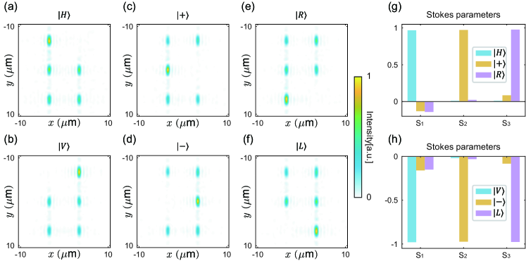
Figure 8: The simulation of intensity at the focal plane. (a)-(f), Spatial distribution of light intensity at the focal plane with input polarizations of $|H\rangle,|V\rangle,|+\rangle,|-\rangle,|R\rangle$ and $|L\rangle$. (g)-(h), The reconstructed Stokes parameters of the input polarizations of $|H\rangle,|V\rangle,|+\rangle,|-\rangle,|R\rangle$ and $|L\rangle$.

D.3 Fabrication of metasurface

A 700nm thick layer of a-Si is deposited on top of $750\mu$m thick fused quartz wafers using the low-pressure chemical vapor deposition (LPCVD) technique. Then a layer of AR-P6200.09 resists (Allresist GmbH) with a thickness of 200nm is spun and coated on the substrate. The metasurface pattern is generated with electron-beam lithography (EBL) process that are set with a 120 kV, 1 nA current, and $300\mu$c/$\text{cm}^{2}$ dose. Subsequently, the resist is developed with AR300-546 (Allresist GmbH) for 1 min. Then reaction ion etching (RIE) is performed to transfer the nanostructures to a-Si film. The residue resist is removed with acetone for 5 min, then isopropanol for 5 min, and finally deionized water. For SEM, a 20nm Au layer was coated and then removed with ceric ammonium nitrate before optical measurement.The SEM images are shown in Fig. 9(a).

D.4 Characterization of metasurface

To characterize the fabricated metasurface, a customized optical system is set up as shown in Fig. 9. The wavelength of the incident light is 810nm followed by a combination of a linear polarizer and a quarter-waveplate (QWP), which could alter the polarization of incident light. Then, the transmitted light through the metasurface focused on the focal plane is captured by a $20\times$ objective lens (OL) and recorded on a CMOS image sensor. The detected power intensity on focal plane with input polarization $|H\rangle,|V\rangle,|+\rangle,|-\rangle,|R\rangle$ and $|L\rangle$ are shown in Fig. 9(b)-(g), and we reconstruct the Stokes parameters with the detected intensity distributions as shown in Fig. 9(h)-(i). The experimental results agree well with simulation results in Fig. 8.

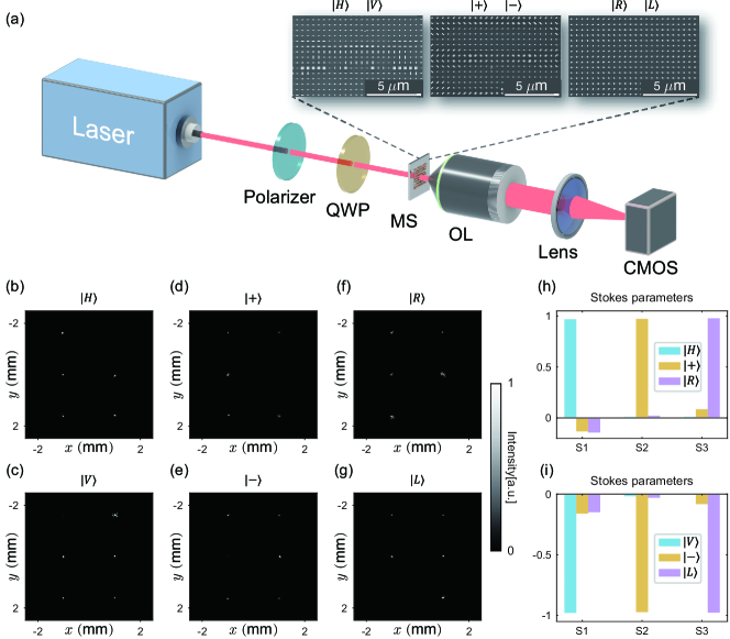
Figure 9: Characterization of the fabricated metasurface. (a), Experimental setup for the metasurface characterization. (b)-(g), The magnified spatial distribution of intensity at the focal plane with different input polarization, which is recorded by a CMOS. (h), (i), Calculated Stokes parameters according to recorded spatial distribution of intensity.

Appendix E More experimental details

E.1 Experimental setup

Metasurface is fixed on a piece of hollow plastic, which can be adjusted in six degrees of freedom through a six-dimensional rotation stage. Objective lens with $20\times$ magnifying factor and tube lens with the focal length of 200mm are used as a microscope, enlarging the distance of six spots focused by metasurface from 70$\mu$m to 1.9mm. After that, three prisms at different height are applied to separate six light beams. To restrain the divergence of beams focused by the microscope and promote the efficiency of beam collection, four mini lens with $f=15$mm and two mini lens with $f=30$mm are set before the fiber couplers. Finally, six beams are coupled into six muti-mode fibers with the core diameter of $62.5\mu$m.

The self-guided quantum tomography (SGQT) on single-photon states requires projective measurement on arbitrary basis, which is realized by a combination of QWP and HWP acting as

$$\begin{split}U_{\text{QWP}}(\delta)&=\frac{1}{\sqrt{2}}\left(\begin{array}[]{cc}1+i\cos 2\delta&i\sin 2\delta\\ i\sin 2\delta&1-i\cos 2\delta\end{array}\right),\\ U_{\text{HWP}}(\delta)&=-\left(\begin{array}[]{cc}\cos 2\delta&\sin 2\delta\\ \sin 2\delta&-\cos 2\delta\end{array}\right).\end{split}$$ (43)

We mount the QWP and HWP on electrical-rotated mounts, and then change the measurement basis at each iteration by electrically rotating the angle of QWP and HWP.