Kinetically Coupled Scalar Fields Model and Cosmological Tensions

Abstract

In this paper, we investigate the kinetically coupled early dark energy (EDE) and scalar field dark matter to address cosmological tensions. The EDE model presents an intriguing theoretical approach to resolving the Hubble tension, but it introduces challenges such as the "why then" problem of why EDE was injected during the epoch of matter-radiation equality, and exacerbates existing large-scale structure tension. Therefore, we consider the interaction between dark matter and EDE, such that the dynamics of EDE are triggered by the dark matter, and the drag effect of dark energy on dark matter suppresses structure growth, which can alleviate large-scale structure tension. We replace cold dark matter with scalar field dark matter, which has the property of suppressing structure growth on small scales. We employed the Markov Chain Monte Carlo method to constrain the model parameters by utilising a variety of cosmological data, our new model reveals a non-zero coupling constant of $0.030\pm 0.026$ at a 68% confidence level. The coupled model yields a Hubble constant value of $72.38^{+0.71}_{-0.82}$  km / s / Mpc, which resolves the Hubble tension. However, similar to the EDE model, it also obtains a larger $S_{8}$ value compared to the $\Lambda$CDM model, further exacerbating the large-scale structure tension. The best-fit $S_{8}$ value for the EDE model is $0.8316$, whereas our new model yields a smaller value of $0.8134$. Additionally, the coupled model exhibits a smaller $\chi^{2}_{\mathrm{tot}}$ value compared to the EDE model and the $\Lambda$CDM model, indicating a better fit to the data.

1 Introduction

The standard $\Lambda$CDM model established over the past decades has received significant support from cosmological data. However, with the continuous improvement of experimental measurements, inconsistencies between some observational results and the predicted results of the $\Lambda$CDM model have become apparent. The most well-known inconsistencies are the Hubble tension and the large-scale structure tension. The Hubble tension refers to the discrepancy in the value of the Hubble constant derived from early universe observations based on the $\Lambda$CDM model and late-time measurements that are independent of the model Verde et al. (2019). Specifically, the best-fit of the $\Lambda$CDM model to the Planck 2018 cosmic microwave background (CMB) data gives $67.37\pm 0.54$ km / s / Mpc Planck Collaboration et al. (2020), whereas the SH0ES collaboration, which uses the distance ladder method at low redshifts, gives $73.04\pm 1.04$ km / s / Mpc Riess et al. (2022), with a statistical error of 4.8$\sigma$ between them.

Another relatively mild tension refers to the inconsistency between the amplitude of density fluctuations $\sigma_{8}$ measured from large-scale structure observations and that measured from CMB observations Macaulay et al. (2013); Hildebrandt et al. (2020). The quantity $S_{8}\equiv\sigma_{8}\sqrt{(\Omega_{m}/0.3)}$ is commonly defined to characterise this tension, where $\Omega_{m}$ denotes the matter energy density fraction. The Planck 2018 best-fit $\Lambda$CDM model yields a value of $S_{8}$ equal to $0.834\pm 0.016$ Planck Collaboration et al. (2020). However, large-scale structure surveys such as the Dark Energy Survey Year-3 (DES-Y3) have reported a smaller value $0.776\pm 0.017$ Abbott et al. (2022).

Currently, it is unclear whether these two tensions stem from unknown statistical errors or inappropriate calibrations Blanchard & Ilić (2021); Mörtsell et al. (2022), or herald new physics beyond the standard model. In any case, it is still meaningful to explore alternative models to the $\Lambda$CDM model and investigate dark matter, dark energy, or dark radiation models that can alleviate these tensions.

Numerous approaches have been proposed to address the Hubble tension, which can be mainly classified into two categories: modifying the physics of the late Universe Guo et al. (2019); Li & Shafieloo (2019); Zhou et al. (2022) and introducing new physics prior to recombination Karwal & Kamionkowski (2016); Poulin et al. (2018); Alexander & McDonough (2019); Lin et al. (2019); Berghaus & Karwal (2020); Ghosh et al. (2020). However, these methods are confronted with various challenges. For instance, the late-time models are competitively constrained by independent observations at low redshift and generally cannot account for SH0ES measurements Benevento et al. (2020); Raveri (2020); Alestas & Perivolaropoulos (2021). Early-time models that achieve relative success in increasing $H_{0}$ often exacerbate the tension in large-scale structure Hill et al. (2020); McDonough et al. (2022). Despite this, the relative success in relieving Hubble tension through modifications to early universe has stimulated further investigation into such models. In this paper, we will focus on one of the most absorbing cases in early models, namely early dark energy (EDE) model Karwal & Kamionkowski (2016); Lin et al. (2019); Poulin et al. (2019), and address its associated issues.

EDE is composed of an ultra-light scalar field, which only make a significant contribution during the epoch approaching matter-radiation equality, and is negligible during other epochs. The addition of a new component decreases the sound horizon at recombination, thereby allowing an increase in the value of $H_{0}$ while keeping the sound horizon angular scale unchanged.

However, obtaining a larger value of $H_{0}$ through the EDE scenario comes at the cost of inducing changes in other cosmological parameters, such as the density of dark matter $\Omega_{\mathrm{c}}h^{2}$, the scalar spectral index $n_{\mathrm{s}}$, and the amplitude of density perturbations $\sigma_{8}$ McDonough et al. (2022). This exacerbates the tension between the model and the large-scale structure data. Additionally, the EDE scalar field necessitates fine-tuning of its parameters, including a small field mass, to ensure that EDE can contribute its energy density at the appropriate time.

One natural idea to address these issues is to introduce the interaction between EDE and dark matter. The drag of dark energy on dark matter can inhibit structure growth, alleviate the large-scale structure tension exacerbated by EDE, and moreover, the emerging dominant component of the universe, dark matter, can trigger the dynamics of EDE, explaining why EDE contributes at a time close to matter-radiation equality Karwal et al. (2022); Lin et al. (2023).

Previous studies have investigated the interaction between EDE and dark matter, such as utilising the Swampland Distance Conjecture Ooguri & Vafa (2007); Klaewer & Palti (2017); Palti (2019) to consider the exponential dependence of the EDE scalar on the mass of dark matter McDonough et al. (2022); Lin et al. (2023); Liu et al. (2023). In this work, inspired by string theory, we consider the kinetic coupling between EDE and scalar field dark matter (SFDM).

SFDM, consisting of a light scalar field with a mass of approximately $10^{-22}$ eV, is a viable alternative to cold dark matter (CDM) Ferreira (2021); Téllez-Tovar et al. (2022). SFDM forms condensates on small scales, which suppress structure growth, while on large scales it exhibits behavior consistent with that of CDM. Fig. 1 illustrates the equation of state with respect to scale factor for SFDM of varying masses. In the early universe, SFDM behaves like a cosmological constant, then undergoes oscillations before ultimately evolving similarly to CDM, and the mass of the scalar field affects the onset time of the oscillation process.

Figure 1: The evolution of the equation of state of scalar field dark matter with respect to the scale factor $a$ is investigated. The evolution of SFDM exhibits behavior similar to a cosmological constant in the early universe, then experiences oscillations, and finally evolves similarly to that of cold dark matter.

The kinetic coupling between two scalar fields has been previously investigated, particularly in relation to the axio-dilaton models Alexander & McDonough (2019); Alexander et al. (2023). In this paper, we introduce a EDE scalar-dependent function to the kinetic term of SFDM, allowing for energy exchange between the two scalar fields. The specific Lagrangian is written as

$$\mathcal{L}_{\mathrm{int}}=-\frac{1}{2}g^{\mu\nu}\partial_{\mu}\phi\partial_{\nu}\phi-V(\phi)-\frac{1}{2}\zeta(\phi)g^{\mu\nu}\partial_{\mu}\chi\partial_{\nu}\chi-V(\chi),$$ (1)

where $\phi$ and $\chi$ represent the EDE scalar and SFDM, respectively. The kinetic term of SFDM is multiplied by the coupling function $\zeta(\phi)$.

We conducted a detailed study of the evolution equations for the kinetically coupled scalar field (KCS) model, including both the background and perturbation parts. We incorporated various commonly used cosmological data, including the Planck 2018 CMB temperature, polarization, and lensing measurements Aghanim et al. (2020a, b); Planck Collaboration et al. (2020); BAO measurements from BOSS DR12, 6dF Galaxy Survey, and SDSS DR7 Beutler et al. (2011); Ross et al. (2015); Alam et al. (2017); Buen-Abad et al. (2018); and the Pantheon supernova Ia sample Scolnic et al. (2018). Additionally, we utilised the measurement of the Hubble constant from SH0ES Riess et al. (2022) and the results of $S_{8}$ from the Dark Energy Survey Year-3 data Abbott et al. (2022).

By employing the Markov Chain Monte Carlo (MCMC) method, we constrained the model parameters. Utilising the entire dataset, the results revealed non-zero coupling constants at a 68% confidence level of $0.030\pm 0.026$. The new model yielded the Hubble constant of $72.38^{+0.71}_{-0.82}$ km / s / Mpc, indicating its capability in addressing the Hubble tension. Similar to the EDE model, the coupling model still obtained a larger $S_{8}$ value compared to the $\Lambda$CDM model, with the best-fit value being $0.8134$. However, this value is smaller than the result obtained by the EDE model, which is $0.8316$. Hence, the new model partially alleviates the negative effects of the EDE model. Furthermore, the KCS model exhibits a smaller $\chi^{2}_{\mathrm{tot}}$ compared to the other two models, indicating a better fit between the model and the data.

The structure of this paper is as follows: Section 2 introduces the KCS model, discussing its dynamics in both the background and perturbation levels, as well as its modifications to the original EDE model. In Section 3, we present the numerical results of the new model, including its impact on the evolution of the Hubble parameter and large-scale structures. Section 4 provides an introduction to the various cosmological data used in the MCMC analysis, along with the resulting parameter constraints. Finally, we summarise our findings in Section 5.

2 Kinetically Coupled Scalar Fields

Considering the Lagrangian shown in equation (1), we employed the potential form of EDE as follows Hill et al. (2020); Smith et al. (2020),

$$V(\phi)=m_{\phi}^{2}f_{\phi}^{2}[1-\cos(\phi/f)]^{3}+V_{\Lambda},$$ (2)

where $m_{\phi}$ represents the axion mass, $f_{\phi}$ denotes its decay constant, and $V_{\Lambda}$ plays the role of a cosmological constant. For SFDM, we assume a simple quadratic potential,

$$V(\chi)=\frac{1}{2}m_{\chi}^{2}\chi^{2},$$ (3)

with $m_{\chi}$ representing the mass of the SFDM. As for the coupling function, a natural choice is to assume an exponential form,

$$\zeta(\phi)=\exp(\frac{\lambda\phi}{M_{pl}}),$$ (4)

where $\lambda$ represents a dimensionless constant that characterises the strength of the interaction, and $M_{pl}$ is the reduced Planck mass.

2.1 Background Equations

The equations of motion for the two scalar fields in a flat Friedmann-Robertson-Walker (FRW) metric can be expressed as

$$\ddot{\phi}+3H\dot{\phi}+V_{\phi}-\frac{1}{2}\frac{\lambda}{M_{pl}}\exp(\frac{\lambda\phi}{M_{pl}})\dot{\chi}^{2}=0,$$ (5a)

$$\ddot{\chi}+(3H+\frac{\lambda\dot{\phi}}{M_{pl}})\dot{\chi}+\exp(-\frac{\lambda\phi}{M_{pl}})m_{\chi}^{2}\chi=0,$$ (5b)

where the dot denotes the derivative with respect to cosmic time, $H$ is the Hubble parameter, and $V_{\phi}$ represents the partial derivative of the EDE potential with respect to $\phi$. It is easy to see that for a non-trivial kinetic coupling function $\zeta(\phi)$, the EDE field has a source term proportional to $\dot{\chi}^{2}$, while the SFDM field has a friction term proportional to $\dot{\phi}$. Therefore, if $\dot{\chi}$ is not equal to zero and the coupling constant $\lambda$ is positive, energy will be transferred from SFDM to EDE.

The energy density and pressure of SFDM can be expressed as

$$\rho_{\chi}=\frac{1}{2}\zeta\dot{\chi}^{2}+\frac{1}{2}m_{\chi}^{2}\chi^{2},$$ (6a)

$$p_{\chi}=\frac{1}{2}\zeta\dot{\chi}^{2}-\frac{1}{2}m_{\chi}^{2}\chi^{2},$$ (6b)

where we abbreviate $\zeta(\phi)$ as $\zeta$. It is convenient to introduce new variables to calculate the motion equation of SFDM Copeland et al. (1998); Ureña-López & Gonzalez-Morales (2016); Cedeño et al. (2017),

$$\sqrt{\Omega_{\chi}}\sin{\frac{\theta}{2}}=\frac{\sqrt{\zeta}\dot{\chi}}{\sqrt{6}M_{pl}H},$$ (7a)

$$\sqrt{\Omega_{\chi}}\cos{\frac{\theta}{2}}=-\frac{m_{\chi}\chi}{\sqrt{6}M_{pl}H},$$ (7b)

$$y_{1}=\frac{2m_{\chi}}{H},$$ (7c)

where $\Omega_{\chi}=\frac{\rho_{\chi}}{3M_{pl}^{2}H^{2}}$ represents the fraction of the dark matter density. Combining with the Friedmann Equation,

$$\frac{\dot{H}}{H^{2}}=-\frac{3}{2}(1+w_{t}),$$ (8)

where $w_{t}$ represents the total equation of state, defined as the ratio of the total pressure to the total energy density. The evolution equation for the new variable is thus formulated as,

$$\frac{\dot{\Omega}_{\chi}}{\Omega_{\chi}}=3H(w_{t}+\cos\theta)+\frac{\lambda\dot{\phi}}{2M_{pl}}(\cos\theta-1),$$ (9a)

$$\dot{\theta}=Hy_{1}\exp(-\frac{\lambda\phi}{2M_{pl}})-(3H+\frac{\lambda\dot{\phi}}{2M_{pl}})\sin\theta,$$ (9b)

$$\dot{y_{1}}=\frac{3}{2}H(1+w_{t})y_{1}.$$ (9c)

If we consider the energy density and pressure of the EDE scalar field,

$$\rho_{\phi}=\frac{1}{2}\dot{\phi}^{2}+V(\phi),$$ (10a)

$$p_{\phi}=\frac{1}{2}\dot{\phi}^{2}-V(\phi),$$ (10b)

combined with equation (6) and using the equations of motion for both fields, we obtain the following continuity equations,

$$\dot{\rho_{\chi}}=-3H(\rho_{\chi}+p_{\chi})-\frac{\lambda\dot{\phi}}{2M_{pl}}\rho_{\chi}(1-\cos\theta),$$ (11a)

$$\dot{\rho_{\phi}}=-3H(\rho_{\phi}+p_{\phi})+\frac{\lambda\dot{\phi}}{2M_{pl}}\rho_{\chi}(1-\cos\theta).$$ (11b)

Many coupled dark energy models exhibit this common structure Olivares et al. (2008); Koyama et al. (2009); Mukherjee & Banerjee (2016); Wang et al. (2016); Yang et al. (2017), which guarantees that the total stress tensor is covariantly conserved.

Fig. 2 illustrates the evolution of the EDE scalar (left panel) and the fraction of the EDE energy density to the total energy density (right panel) with respect to the scale factor.

Figure 2: The evolution of the EDE scalar (left panel) and the EDE energy density fraction (right panel) with respect to the scale factor is presented. The amplitude and phase of the EDE scalar are modulated by different coupling constants. Positive coupling constants indicate that energy flows from dark matter to dark energy, thereby increasing the energy density fraction of EDE, while negative coupling constants lead to a decrease in the energy density fraction of EDE.

The remaining cosmological parameters are taken from the best-fit values in Table 1. Slight variations in the amplitude and phase of the evolution of the EDE scalar field are induced by different coupling constants. The sign of the coupling constant determines the direction of energy transfer. Positive coupling constants indicate energy flow from dark matter to dark energy, resulting in an increase in the energy density fraction of EDE, as demonstrated in the right panel of the figure.

2.2 Perturbution Equations

We employ the synchronous gauge to compute the perturbation equations for both EDE and SFDM. The line element is defined as,

$$ds^{2}=-dt^{2}+a^{2}(t)(\delta_{ij}+h_{ij})dx^{i}dx^{j}.$$ (12)

The perturbed Klein-Gordon equation in the Fourier mode are given by

$$\begin{split}\ddot{\delta\phi}&=-3H\dot{\delta\phi}-[\frac{k^{2}}{a^{2}}+V_{\phi\phi}-\frac{1}{2}(\frac{\lambda}{M_{pl}})^{2}\exp(\frac{\lambda\phi}{M_{pl}})\dot{\chi}^{2}]\delta\phi\\ &-\frac{1}{2}\dot{h}\dot{\phi}+\frac{\lambda}{M_{pl}}\exp(\frac{\lambda\phi}{M_{pl}})\dot{\chi}\dot{\delta\chi},\end{split}$$ (13)

$$\begin{split}\ddot{\delta\chi}&=-(3H+\frac{\lambda\dot{\phi}}{M_{pl}})\dot{\delta\chi}-[\frac{k^{2}}{a^{2}}+m_{\chi}^{2}\exp(-\frac{\lambda\phi}{M_{pl}})]\delta\chi-\frac{1}{2}\dot{h}\dot{\chi}\\ &+\frac{\lambda}{M_{pl}}[m_{\chi}^{2}\chi\exp(-\frac{\lambda\phi}{M_{pl}})\delta\phi-\dot{\chi}\dot{\delta\phi}],\end{split}$$ (14)

where $V_{\phi\phi}$ represents the second order partial derivative of the EDE potential with respect to $\phi$.

According to Ferreira & Joyce (1998); Hu (1998), the density perturbation, pressure perturbation, and velocity divergence of SFDM can be expressed as,

$$\delta\rho_{\chi}=\zeta\dot{\chi}\dot{\delta\chi}+m_{\chi}^{2}\chi\delta\chi,$$ (15a)

$$\delta p_{\chi}=\zeta\dot{\chi}\dot{\delta\chi}-m_{\chi}^{2}\chi\delta\chi,$$ (15b)

$$(\rho_{\chi}+p_{\chi})\Theta_{\chi}=\frac{k^{2}}{a}\zeta\dot{\chi}\delta\chi.$$ (15c)

We employ some new variables to compute the perturbation equations of SFDM Cedeño et al. (2017),

$$\sqrt{\Omega_{\chi}}(\delta_{0}\sin{\frac{\theta}{2}}+\delta_{1}\cos{\frac{\theta}{2}})=\sqrt{\frac{2}{3}}\frac{\sqrt{\zeta}\dot{\delta\chi}}{M_{pl}H},$$ (16a)

$$\sqrt{\Omega_{\chi}}(\delta_{1}\sin{\frac{\theta}{2}}-\delta_{0}\cos{\frac{\theta}{2}})=\sqrt{\frac{2}{3}}\frac{m_{\chi}\delta\chi}{M_{pl}H}.$$ (16b)

One can derive the evolution equation for the new variable,

$$\begin{split}\dot{\delta_{0}}&=-\frac{\lambda Hy_{1}\delta\phi}{2M_{pl}\sqrt{\zeta}}\sin\theta-(\frac{\lambda\dot{\delta\phi}}{M_{pl}}+\frac{1}{2}\dot{h})(1-\cos\theta)\\ &+\delta_{0}H\omega\sin\theta-\delta_{1}[(3H+\frac{\lambda\dot{\phi}}{2M_{pl}})\sin\theta+H\omega(1-\cos\theta)],\end{split}$$ (17)

$$\begin{split}\dot{\delta_{1}}&=-\frac{\lambda Hy_{1}\delta\phi}{2M_{pl}\sqrt{\zeta}}(1+\cos\theta)-(\frac{\lambda\dot{\delta\phi}}{M_{pl}}+\frac{1}{2}\dot{h})\sin\theta\\ &+\delta_{0}H\omega(1+\cos\theta)-\delta_{1}[(3H+\frac{\lambda\dot{\phi}}{2M_{pl}})\cos\theta+H\omega\sin\theta],\end{split}$$ (18)

where

$$\omega=\frac{k^{2}\sqrt{\zeta}}{2a^{2}m_{\chi}H}=\frac{k^{2}\sqrt{\zeta}}{a^{2}H^{2}y_{1}}.$$ (19)

The relationship between the density perturbations, pressure perturbations, and velocity divergence of SFDM and the new variables can be deduced from equation (15),

$$\delta\rho_{\chi}=\rho_{\chi}\delta_{0},$$ (20a)

$$\delta p_{\chi}=\rho_{\chi}(\delta_{1}\sin\theta-\delta_{0}\cos\theta),$$ (20b)

$$(\rho_{\chi}+p_{\chi})\Theta_{\chi}=\frac{k^{2}\sqrt{\zeta}}{aHy_{1}}\rho_{\chi}[\delta_{1}(1-\cos\theta)-\delta_{0}\sin\theta].$$ (20c)

2.3 Initial Conditions

In the early universe, Hubble friction in the scalar fields dominated and both EDE and SFDM were effectively frozen, undergoing a slow-roll process. The initial value of $\dot{\phi}$ can be set to zero, the term in the EDE equation containing $\dot{\chi}$ can be neglected during that period. Therefore, the equations of motion for EDE and SFDM simplify to an uncoupled form (the equation for the new variable $\theta$ is an exception, and we will address this point later). We introduce the ratio of the initial value of the EDE scalar to the axion decay constant, $\alpha_{i}=\phi_{i}/f_{\phi}$ as the model parameter Hill et al. (2020); Smith et al. (2020). We refer to the initial conditions of uncoupled SFDM and make modifications,

$$y_{1i}=\frac{2m_{\chi}}{H_{0}\sqrt{\Omega_{r}a_{i}^{-4}}},\quad\theta_{i}=\frac{1}{5}y_{1i}\exp{(\frac{-\lambda\phi_{i}}{2M_{pl}})},$$ (21)

where $\Omega_{r}$ represents the energy density fraction of all radiation components at present, and $a_{i}$ denotes the initial value of the scale factor. It should be noted that due to coupling, the initial value of $\theta$ is multiplied by an additional factor, $\exp{\frac{-\lambda\phi_{i}}{2M_{pl}}}$. For the derivation of the initial conditions of the original SFDM model, please refer to Ureña-López & Gonzalez-Morales (2016); Cedeño et al. (2017). Based on the current value of the dark matter energy density, we employ the widely used shooting method in the Boltzmann code CLASS Blas et al. (2011); Lesgourgues (2011) to obtain the initial value of $\Omega_{\chi}$. For the perturbation equations of EDE and SFDM, we employ adiabatic initial conditions, with detailed descriptions provided in Smith et al. (2020) and Cedeño et al. (2017).

3 Numerical Results

Based on the description provided in the previous section, we modified the publicly available Boltzmann code CLASS Blas et al. (2011); Lesgourgues (2011) to incorporate the new model. We present the numerical results where the cosmological parameters adopted by different models are obtained from the best-fit values listed in Tab. 1.

We demonstrate the redshift evolution of the Hubble parameter for various models in Fig. 3. The dashed black line corresponds to the $\Lambda$CDM model, while the dash-dotted blue and solid orange lines represent the EDE model and KCS model, respectively. The 38 data points are obtained from Farooq et al. (2017).

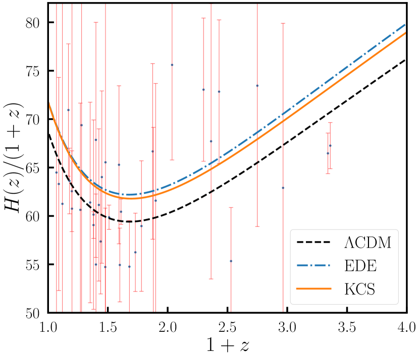
Figure 3: The evolution of the Hubble parameter with redshift varies among different models. The inclusion of an early dark energy component in the EDE and KCS models results in higher values of the Hubble parameter compared to the $\Lambda$CDM model. In the KCS model, the interaction between dark matter and dark energy results in a lower Hubble parameter during the matter-dominated era compared to the EDE model.

The presence of an early dark energy component in both the EDE and KCS models leads to higher values of the Hubble parameter compared to the $\Lambda$CDM model. In the KCS model, the energy density during the matter-dominated era is smaller than that in the EDE model due to the continuous conversion of dark matter into dark energy. However, after entering the dark energy-dominated phase, the differences between the two models diminish, eventually converging to similar values of the Hubble constant.

Fig. 4 illustrates the redshift evolution of $f\sigma_{8}$ for three different models. The 63 observed Redshift Space Distortion $f\sigma_{8}(z)$ data points are gathered from Kazantzidis & Perivolaropoulos (2018).

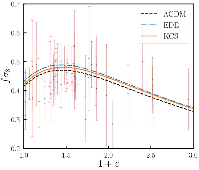
Figure 4: The redshift evolution of $f\sigma_{8}$ for the three models is examined. The $f\sigma_{8}$ obtained from the EDE model and KCS model are higher than the $\Lambda$CDM model. Compared to the EDE model, the $f\sigma_{8}$ in the KCS model is lower, primarily due to the interplay between dark matter and dark energy, as well as the condensation characteristics of SFDM on small scales.

Both the EDE and KCS models yield higher $f\sigma_{8}$ compared to the $\Lambda$CDM model, exacerbating the existing $S_{8}$ tension. Fortunately, in the KCS model, the suppression of structure growth on small scales due to SFDM and the dragging of dark matter by dark energy lead to a lower $f\sigma_{8}$ compared to the EDE model, partially alleviating the negative effects of EDE.

In Fig. 5, we present the linear matter power spectra for three models (top panel) and the differences between the power spectra of various models relative to the $\Lambda$CDM model (bottom panel).

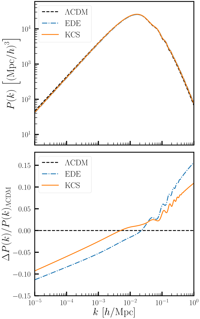
Figure 5: The linear matter power spectra of three models (top panel) and their deviations from the $\Lambda$CDM model (bottom panel) are presented. The reduced matter power spectrum of the KCS model on small scales is attributed to the interaction between dark matter and dark energy, as well as the condensation of SFDM on small scales.

Compared to the EDE model, the KCS model exhibits a noticeable difference in that its matter power spectrum is smaller on small scales. This can mainly be attributed to the interplay between dark matter and dark energy, which results in a decrease in the energy density of dark matter, weakening the degree of matter clumping and resulting in smaller matter density fraction $\Omega_{\mathrm{m}}$ and density fluctuation amplitudes $\sigma_{8}$.

In addition, the condensation of SFDM on galactic scales also suppresses the growth of structure on small scales. Consequently, the new model obtains a smaller $S_{8}$ value compared to the EDE model, thus mitigating the issues associated with the EDE model.

4 Data and Methodology

We conducted a Markov Chain Monte Carlo (MCMC) analysis using MontePython Audren et al. (2013); Brinckmann & Lesgourgues (2018) to obtain the posterior distribution of the model parameters, and assessed convergence using the Gelman-Rubin criterion Gelman & Rubin (1992), $R-1<0.05$. The MCMC chains were analysed using GetDist Lewis (2019).

4.1 Datasets

To perform the MCMC analysis, we used the following datasets:

• CMB: The temperature and polarization power spectra obtained from the Planck 2018 low-$\ell$ and high-$\ell$ measurements, as well as the CMB lensing power spectrum Aghanim et al. (2020a, b); Planck Collaboration et al. (2020).

• BAO: The measurements obtained from the BOSS-DR12 $f\sigma_{8}$ sample comprise the combined LOWZ and CMASS galaxy samples Alam et al. (2017); Buen-Abad et al. (2018), as well as the small-z measurements derived from 6dFGS and the SDSS DR7 Beutler et al. (2011); Ross et al. (2015).

• Supernovae: The Pantheon dataset consists of 1048 supernovae type Ia with redshift values ranging from 0.01 to 2.3 Scolnic et al. (2018).

By combining CMB and BAO data, acoustic horizon measurements can be made at multiple redshifts, breaking geometric degeneracies and constraining the physical processes between recombination and the redshift at which BAO is measured. The supernova data obtained from the Pantheon sample significantly constrains late-time new physic within its measured redshift range.

• SH0ES: According to the latest SH0ES measurement, the value of the Hubble constant is estimated to be $73.04\pm 1.04$ km / s / Mpc Riess et al. (2022).

• DES-Y3: The Dark Energy Survey Year-3 has yielded valuable data on weak lensing and galaxy clustering, from which the parameter $S_{8}$ has been measured to be $0.776\pm 0.017$ Abbott et al. (2022).

We employ the $H_{0}$ measurements from SH0ES to alleviate the prior volume effect Smith et al. (2021) and assess the ability of the novel model to mitigate the tension between $H_{0}$ local measurement and CMB inference result. Additionally, we incorporate the $S_{8}$ data from DES-Y3 to investigate the efficacy of the model in easing the large-scale structure tension.

4.2 Results

The results of parameter constraints are presented in Tab. 1, where we utilised a comprehensive dataset comprising CMB, BAO, SNIa, SH0ES, and $S_{8}$ from DES-Y3 data to individually constrain the $\Lambda$CDM, EDE, and KCS models.

Table 1: The table illustrates the best-fit parameters and 68% confidence level marginalized constraints for the $\Lambda$CDM, EDE, and KCS models. These constraints are derived from comprehensive data sets including CMB, BAO, SNIa, SH0ES, and $S_{8}$ measurements obtained from DES-Y3. The upper portion of the table consists of the cosmological parameters that were explored using MCMC sampling, while the lower portion presents the derived parameters.

Model	$\Lambda$CDM	EDE	KCS
$100\omega{}_{\mathrm{b}}$	$2.269(2.263\pm 0.014)$	$2.276(2.281^{+0.024}_{-0.020})$	$2.290(2.281\pm 0.020)$
$\omega{}_{\mathrm{dm}}$	$0.11724(0.11725\pm 0.00084)$	$0.1310(0.1299\pm 0.0028)$	$0.1272(0.1303\pm 0.0028)$
$H_{0}$	$68.73(68.71^{+0.35}_{-0.41})$	$71.85(72.46\pm 0.86)$	$71.81(72.38^{+0.71}_{-0.82})$
$\ln(10^{10}A_{\mathrm{s}})$	$3.043(3.050\pm 0.015)$	$3.057(3.063^{+0.015}_{-0.017})$	$3.057(3.057\pm 0.018)$
$n_{\mathrm{s}}$	$0.9736(0.9722\pm 0.0040)$	$0.9877(0.9908\pm 0.0059)$	$0.9891(0.9875^{+0.0065}_{-0.0041})$
$\tau{}_{\mathrm{reio}}$	$0.0574(0.0592\pm 0.0082)$	$0.0539(0.0563\pm 0.0090)$	$0.0578(0.0543\pm 0.0093)$
$\log_{10}(m_{\phi})$	$-$	$-27.292(-27.290\pm 0.055)$	$-27.314(-27.295^{+0.052}_{-0.042})$
$\log_{10}(f_{\phi})$	$-$	$26.632(26.616^{+0.056}_{-0.033})$	$26.637(26.645\pm 0.051)$
$\alpha_{\mathrm{i}}$	$-$	$2.762(2.783\pm 0.069)$	$2.650(2.696^{+0.069}_{-0.055})$
$\lambda$	$-$	$-$	$0.0171(0.030\pm 0.026)$
$\log_{10}(m_{\chi})$	$-$	$-$	$-21.823(-21.988\pm 0.063)$
$10^{-9}A_{\mathrm{s}}$	$2.096(2.112\pm 0.032)$	$2.127(2.139^{+0.031}_{-0.036})$	$2.127(2.127\pm 0.038)$
$100\theta{}_{\mathrm{s}}$	$1.04206(1.04217^{+0.00025}_{-0.00031})$	$1.04121(1.04145\pm 0.00043)$	$1.04146(1.04140^{+0.00028}_{-0.00039})$
$f_{\mathrm{EDE}}$	$-$	$0.1183(0.119^{+0.023}_{-0.018})$	$0.1004(0.124\pm 0.021)$
$\log_{10}(z_{\mathrm{c}})$	$-$	$3.571(3.568\pm 0.034)$	$3.572(3.569^{+0.028}_{-0.025})$
$\Omega{}_{\mathrm{m}}$	$0.2976(0.2977\pm 0.0048)$	$0.2991(0.2923\pm 0.0056)$	$0.2924(0.2935^{+0.0057}_{-0.0043})$
$\sigma_{8}$	$0.8017(0.8047\pm 0.0060)$	$0.8329(0.8325\pm 0.0083)$	$0.8239(0.8284^{+0.0088}_{-0.0071})$
$S_{8}$	$0.7985(0.8016^{+0.0096}_{-0.0080})$	$0.8316(0.822^{+0.011}_{-0.0093})$	$0.8134(0.819^{+0.013}_{-0.0092})$
$\Delta\chi^{2}_{\mathrm{tot}}$	$-$	$-11.74$	$-12.78$

The upper segment of the table represents the parameters subjected to MCMC sampling, while the lower segment displays the derived parameters.

Firstly, it is noteworthy that the KCS model constrains the coupling constant $\lambda$ to be $0.030\pm 0.026$ at a 68% confidence level, with a best-fit value of 0.0171. This indicates an interaction between dark matter and dark energy, specifically the conversion of dark matter to dark energy.

From the perspective of the Hubble constant, the EDE model and KCS model yield $H_{0}$ values of $72.46\pm 0.86$ km / s / Mpc and $72.38^{+0.71}_{-0.82}$ km / s / Mpc, respectively, at a 68% confidence level, both of which exceed the value of $68.71^{+0.35}_{-0.41}$ km / s / Mpc obtained by the $\Lambda$CDM model. Therefore, both the EDE model and KCS model demonstrate the capacity to address the Hubble tension.

However, the performance of both models on $S_{8}$ is suboptimal. The best-fit values of $S_{8}$ for the EDE and KCS models are 0.8316 and 0.8134, respectively, whereas $\Lambda$CDM yields a result of 0.7985. Both models exacerbate the preexisting $S_{8}$ tension. Nevertheless, the KCS model demonstrates relatively superior performance compared to the EDE model, benefiting from the condensation effect of SFDM on small scales, as well as the interplay between dark matter and dark energy. Consequently, the KCS model exhibits a smaller $S_{8}$, partially alleviating the negative effects in the EDE model.

These discussions can be visually depicted in the marginalized posterior distributions of various models, as illustrated in Fig. 6. The complete posterior distributions can be found in Fig. 7 in the Appendix section.

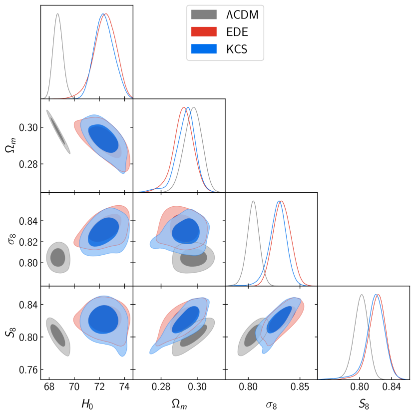
Figure 6: The marginalized posterior distributions of the three models are presented. Both the EDE and KCS models yield larger values of $H_{0}$ and hence, a larger $S_{8}$ compared to the $\Lambda$CDM model. However, the KCS model partially alleviates the $S_{8}$ tension when compared to the EDE model.

The last row of Tab. 1 presents the $\Delta\chi^{2}_{\mathrm{tot}}$ values for the EDE and KCS models with respect to the $\Lambda$CDM model, which are -11.74 and -12.78, respectively. Both models exhibit significantly reduced $\chi^{2}_{\mathrm{tot}}$ values compared to the $\Lambda$CDM model, primarily due to the contribution from the SH0ES data. Furthermore, the KCS model demonstrates a lower $\chi^{2}_{\mathrm{tot}}$ value than the EDE model, attributed to its smaller $S_{8}$ value, which better aligns with the DES-Y3 data.

5 Conclusions

In this paper, we investigate the interaction between early dark energy (EDE) and scalar field dark matter (SFDM), proposing a kinetically coupled scalar fields (KCS) model to alleviate cosmological tensions. The EDE model offers a resolution to the Hubble tension, but exacerbates the $S_{8}$ tension and lacks an explanation for its presence during a specific epoch, namely the period near matter-radiation equality.

In light of this, we propose an interaction between dark matter and dark energy, aiming to alleviate the $S_{8}$ tension through the drag exerted by dark energy on dark matter. Additionally, we hypothesise that the dynamical behavior of EDE can be triggered by dark matter, which was poised to become the dominant component of the universe.

In particular, motivated by the ability of SFDM to suppress structure growth on small scales, we replace cold dark matter with SFDM. Inspired by string theory, we consider a kinetic coupling between two scalar fields, where the kinetic term of SFDM is multiplied by an EDE scalar-dependent function.

We derived the evolution equations of the KCS model at both the background and perturbation levels, and investigated its impact on the evolution of the Hubble parameter, as well as on the structure growth and matter power spectrum. By using cosmological data from various sources, including the CMB, BAO, SNIa, the SH0ES measurement of the Hubble constant, and the DES-Y3 observations, we conducted MCMC analysis.

We obtained a non-zero coupling constant $\lambda$ of $0.030\pm 0.026$ at a 68% confidence level. This suggests the interaction between dark matter and dark energy, with energy transferring from dark matter to dark energy. The values of $H_{0}$ of the EDE model and KCS model are $72.46\pm 0.86$ km / s / Mpc and $72.38^{+0.71}_{-0.82}$ km / s / Mpc, respectively, while the result of $\Lambda$CDM model is $68.71^{+0.35}_{-0.41}$ km / s / Mpc. Both models alleviate the Hubble tension.

However, the corresponding cost is that both the EDE model and KCS model yield larger values of $S_{8}$, with their best-fit values being 0.8316 and 0.8134, respectively, which are greater than the result of the $\Lambda$CDM model, 0.7985. Nevertheless, compared to the EDE model, the KCS model performs slightly better. This can be primarily attributed to the drag exerted by dark energy on dark matter in the new model, as well as the condensation effect of SFDM on small scales, both of which inhibit structure growth.

Moreover, in terms of the goodness-of-fit to the data, the $\chi^{2}_{\mathrm{tot}}$ values for the EDE model and KCS model relative to the $\Lambda$CDM model are -11.74 and -12.78, respectively. It can be observed that the KCS model demonstrates superior performance in fitting the data.

Building upon the EDE model, we considered the coupling between dark matter and dark energy, which mitigates the negative effects inherent in the EDE model. However, the KCS model still falls short of fully resolving all cosmological tensions. Further efforts are still required to address these challenges comprehensively.

Data Availability

The data supporting the findings of this article are available upon reasonable request to the corresponding author.

Appendix A The Full MCMC posteriors

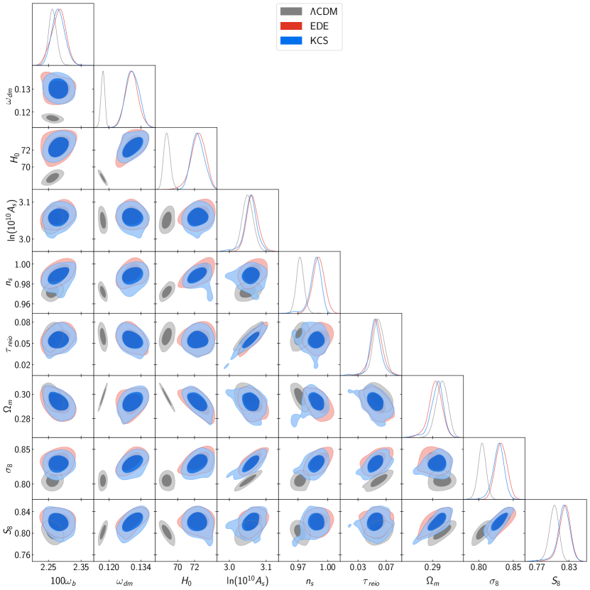
Figure 7: The complete posterior distributions for $\Lambda$CDM, EDE, and KCS models with data comprising CMB, BAO, SNIa, SH0ES, and $S_{8}$ from DES-Y3.

References

- Abbott et al. (2022) Abbott T. M. C., Aguena M., Alarcon A., et al., 2022, Phys. Rev. D, 105, 023520
- Aghanim et al. (2020b) Aghanim N., Akrami Y., Ashdown M., et al., 2020b, Astronomy and Astrophysics, 641
- Aghanim et al. (2020a) Aghanim N., Akrami Y., Ashdown M., et al., 2020a, Astronomy and Astrophysics, 641
- Alam et al. (2017) Alam S., Ata M., Bailey S., et al., 2017, Monthly Notices of the Royal Astronomical Society, 470, 2617
- Alestas & Perivolaropoulos (2021) Alestas G., Perivolaropoulos L., 2021, Monthly Notices of the Royal Astronomical Society, 504, 3956
- Alexander & McDonough (2019) Alexander S., McDonough E., 2019, Physics Letters B, 797, 134830
- Alexander et al. (2023) Alexander S., Bernardo H., Toomey M. W., 2023, Journal of Cosmology and Astroparticle Physics, 2023, 037
- Audren et al. (2013) Audren B., Lesgourgues J., Benabed K., Prunet S., 2013, Journal of Cosmology and Astroparticle Physics, 2013, 001
- Benevento et al. (2020) Benevento G., Hu W., Raveri M., 2020, Phys. Rev. D, 101, 103517
- Berghaus & Karwal (2020) Berghaus K. V., Karwal T., 2020, Phys. Rev. D, 101, 083537
- Beutler et al. (2011) Beutler F., Blake C., Colless M., et al., 2011, Monthly Notices of the Royal Astronomical Society, 416, 3017
- Blanchard & Ilić (2021) Blanchard A., Ilić S., 2021, Astronomy and Astrophysics, 656, A75
- Blas et al. (2011) Blas D., Lesgourgues J., Tram T., 2011, Journal of Cosmology and Astroparticle Physics, 2011, 034
- Brinckmann & Lesgourgues (2018) Brinckmann T., Lesgourgues J., 2018, MontePython 3: boosted MCMC sampler and other features (arXiv:1804.07261)
- Buen-Abad et al. (2018) Buen-Abad M. A., Schmaltz M., Lesgourgues J., Brinckmann T., 2018, Journal of Cosmology and Astroparticle Physics, 2018, 008
- Cedeño et al. (2017) Cedeño F. X. L., González-Morales A. X., Ureña López L. A., 2017, Phys. Rev. D, 96, 061301
- Copeland et al. (1998) Copeland E. J., Liddle A. R., Wands D., 1998, Phys. Rev. D, 57, 4686
- Farooq et al. (2017) Farooq O., Madiyar F. R., Crandall S., Ratra B., 2017, The Astrophysical Journal, 835, 26
- Ferreira (2021) Ferreira E. G. M., 2021, The Astronomy and Astrophysics Review, 29
- Ferreira & Joyce (1998) Ferreira P. G., Joyce M., 1998, Phys. Rev. D, 58, 023503
- Gelman & Rubin (1992) Gelman A., Rubin D. B., 1992, Statistical Science, 7, 457
- Ghosh et al. (2020) Ghosh S., Khatri R., Roy T. S., 2020, Phys. Rev. D, 102, 123544
- Guo et al. (2019) Guo R.-Y., Zhang J.-F., Zhang X., 2019, Journal of Cosmology and Astroparticle Physics, 2019, 054
- Hildebrandt et al. (2020) Hildebrandt H., Köhlinger F., Busch J., et al., 2020, Astronomy & Astrophysics, 633, A69
- Hill et al. (2020) Hill J. C., McDonough E., Toomey M. W., Alexander S., 2020, Phys. Rev. D, 102, 043507
- Hu (1998) Hu W., 1998, The Astrophysical Journal, 506, 485
- Karwal & Kamionkowski (2016) Karwal T., Kamionkowski M., 2016, Phys. Rev. D, 94, 103523
- Karwal et al. (2022) Karwal T., Raveri M., Jain B., Khoury J., Trodden M., 2022, Phys. Rev. D, 105, 063535
- Kazantzidis & Perivolaropoulos (2018) Kazantzidis L., Perivolaropoulos L., 2018, Phys. Rev. D, 97, 103503
- Klaewer & Palti (2017) Klaewer D., Palti E., 2017, Journal of High Energy Physics, 2017
- Koyama et al. (2009) Koyama K., Maartens R., Song Y.-S., 2009, Journal of Cosmology and Astroparticle Physics, 2009, 017
- Lesgourgues (2011) Lesgourgues J., 2011, The Cosmic Linear Anisotropy Solving System (CLASS) I: Overview (arXiv:1104.2932)
- Lewis (2019) Lewis A., 2019, GetDist: a Python package for analysing Monte Carlo samples (arXiv:1910.13970)
- Li & Shafieloo (2019) Li X., Shafieloo A., 2019, The Astrophysical Journal Letters, 883, L3
- Lin et al. (2019) Lin M.-X., Benevento G., Hu W., Raveri M., 2019, Phys. Rev. D, 100, 063542
- Lin et al. (2023) Lin M.-X., McDonough E., Hill J. C., Hu W., 2023, Phys. Rev. D, 107, 103523
- Liu et al. (2023) Liu G., Zhou Z., Mu Y., Xu L., 2023, Alleviating Cosmological Tensions with a Coupled Scalar Fields Model (arXiv:2307.07228)
- Macaulay et al. (2013) Macaulay E., Wehus I. K., Eriksen H. K., 2013, Phys. Rev. Lett., 111, 161301
- McDonough et al. (2022) McDonough E., Lin M.-X., Hill J. C., Hu W., Zhou S., 2022, Phys. Rev. D, 106, 043525
- Mukherjee & Banerjee (2016) Mukherjee A., Banerjee N., 2016, Classical and Quantum Gravity, 34
- Mörtsell et al. (2022) Mörtsell E., Goobar A., Johansson J., Dhawan S., 2022, The Astrophysical Journal, 933, 212
- Olivares et al. (2008) Olivares G., Atrio-Barandela F., Pavón D., 2008, Phys. Rev. D, 77, 063513
- Ooguri & Vafa (2007) Ooguri H., Vafa C., 2007, Nuclear Physics B, 766, 21
- Palti (2019) Palti E., 2019, Fortschritte der Physik, 67
- Planck Collaboration et al. (2020) Planck Collaboration Aghanim, N. Akrami, Y. et al., 2020, Astronomy and Astrophysics, 641, A6
- Poulin et al. (2018) Poulin V., Smith T. L., Grin D., Karwal T., Kamionkowski M., 2018, Phys. Rev. D, 98, 083525
- Poulin et al. (2019) Poulin V., Smith T. L., Karwal T., Kamionkowski M., 2019, Phys. Rev. Lett., 122, 221301
- Raveri (2020) Raveri M., 2020, Phys. Rev. D, 101, 083524
- Riess et al. (2022) Riess A. G., et al., 2022, The Astrophysical Journal Letters, 934, L7
- Ross et al. (2015) Ross A. J., Samushia L., Howlett C., et al., 2015, Monthly Notices of the Royal Astronomical Society, 449, 835
- Scolnic et al. (2018) Scolnic D. M., Jones D. O., Rest A., Pan Y. C., et al., 2018, The Astrophysical Journal, 859, 101
- Smith et al. (2020) Smith T. L., Poulin V., Amin M. A., 2020, Phys. Rev. D, 101, 063523
- Smith et al. (2021) Smith T. L., Poulin V., Bernal J. L., Boddy K. K., Kamionkowski M., Murgia R., 2021, Phys. Rev. D, 103, 123542
- Téllez-Tovar et al. (2022) Téllez-Tovar L. O., Matos T., Vázquez J. A., 2022, Phys. Rev. D, 106, 123501
- Ureña-López & Gonzalez-Morales (2016) Ureña-López L. A., Gonzalez-Morales A. X., 2016, Journal of Cosmology and Astroparticle Physics, 2016, 048
- Verde et al. (2019) Verde L., Treu T., Riess A. G., 2019, Nature Astronomy, 3, 891
- Wang et al. (2016) Wang B., Abdalla E., Atrio-Barandela F., Pavón D., 2016, Reports on Progress in Physics, 79, 096901
- Yang et al. (2017) Yang W., Pan S., Mota D. F., 2017, Phys. Rev. D, 96, 123508
- Zhou et al. (2022) Zhou Z., Liu G., Mu Y., Xu L., 2022, Monthly Notices of the Royal Astronomical Society, 511, 595