SynJax: Structured Probability Distributions for JAX

Abstract

The development of deep learning software libraries enabled significant progress in the field by allowing users to focus on modeling, while letting the library to take care of the tedious and time-consuming task of optimizing execution for modern hardware accelerators. However, this has benefited only particular types of deep learning models, such as Transformers, whose primitives map easily to the vectorized computation. The models that explicitly account for structured objects, such as trees and segmentations, did not benefit equally because they require custom algorithms that are difficult to implement in a vectorized form.

SynJax directly addresses this problem by providing an efficient vectorized implementation of inference algorithms for structured distributions covering alignment, tagging, segmentation, constituency trees and spanning trees. This is done by exploiting the connection between algorithms for automatic differentiation and probabilistic inference. With SynJax we can build large-scale differentiable models that explicitly model structure in the data. The code is available at https://github.com/google-deepmind/synjax.

1 Introduction

In many domains, data can be seen as having some structure explaining how its parts fit into a larger whole. This structure is often latent, and it varies depending on the task. For examples of discrete structures in natural language consider Figure 1. The words together form a sequence. Each word in a sequence is assigned a part-of-speech tag. These tags are dependent on each other, forming a linear-chain marked in red. The words in the sentence can be grouped together into small disjoint contiguous groups by sentence segmentation, shown with bubbles. A deeper analysis of language would show that the groupings can be done recursively and thereby produce a syntactic tree structure. Structures can also relate two languages. For instance, in the same figure, a Japanese translation can be mapped to an English source by an alignment.

These structures are not specific to language. Similar structures appear in biology as well. Nucleotides of any two RNA sequences are matched with monotone alignment (Needleman and Wunsch, 1970; Wang and Xu, 2011), genomic data is segmented into contiguous groups (Day et al., 2007) and tree-based models of RNA capture the hierarchical nature of the protein folding process (Sakakibara et al., 1994; Hockenmaier et al., 2007; Huang et al., 2019).

for tree=s sep=10mm, inner sep=0, l=0 [S [NP,tier=first [D
The,align=center,tier=words,name=A] [N
dog,align=center,tier=words,name=B] ] [VP [V
chases,align=center,tier=words,name=C] [NP,tier=first [D
a,align=center,tier=words,name=D] [N
cat,align=center,tier=words,name=E] ] ] ] [draw,rounded rectangle,fit=(A) (B),fill=blue,opacity=.2] (AB) ; [draw,rounded rectangle,fit=(C),fill=blue,opacity=.2] (CC) ; [draw,rounded rectangle,fit=(D) (E),fill=blue,opacity=.2] (DE) ; [below =of D,draw,rounded rectangle,fill=yellow,opacity=.2,text opacity=1.] (CO) 追いかけている ; [left = 0.5cm of CO,draw,rounded rectangle,fill=yellow,opacity=.2,text opacity=1.] (BO) 猫を ; [left = 0.5cm of BO,draw,rounded rectangle,fill=yellow,opacity=.2,text opacity=1.] (AO) 犬が ; [-=] (AB.south) to (AO.north); [-=] (DE.south west) to[out=210,in=20] (BO.north east); [-=] (CC.south) to (CO); [-¿,dotted,red,very thick] ($(A.east)+(0,0.3)$) to ($(B.west)+(0,0.3)$); [-¿,dotted,red,very thick] ($(B.east)+(0,0.3)$) to ($(C.west)+(0.3,0.3)$); [-¿,dotted,red,very thick] ($(C.east)+(0,0.3)$) to ($(D.west)+(-0.1,0.3)$); [-¿,dotted,red,very thick] ($(D.east)+(0.1,0.3)$) to ($(E.west)+(0,0.3)$);

Figure 1: Examples of natural language structures.

Most contemporary deep learning models attempt to predict output variables directly from the input without any explicit modeling of the intermediate structure. Modeling structure explicitly could improve these models in multiple ways. First, it could allow for better generalization trough the right inductive biases (Dyer et al., 2016; Sartran et al., 2022). This would improve not only sample efficiency but also downstream performance (Bastings et al., 2017; Nădejde et al., 2017; Bisk and Tran, 2018). Explicit modeling of structure can also enable incorporation of problem specific algorithms (e.g. finding shortest paths; Pogančić et al., 2020; Niepert et al., 2021) or constraints (e.g. enforcing alignment Mena et al., 2018 or enforcing compositional calculation Havrylov et al., 2019). Discrete structure also allows for better interpretability of the model’s decisions (Bastings et al., 2019). Finally, sometimes structure is the end goal of learning itself – for example we may know that there is a hidden structure of a particular form explaining the data, but its specifics are not known and need to be discovered (Kim et al., 2019; Paulus et al., 2020).

Auto-regressive models are the main approach used for modeling sequences. Non-sequential structures are sometimes linearized and approximated with a sequential structure (Choe and Charniak, 2016). These models are powerful as they do not make any independence assumptions and can be trained on large amounts of data. While sampling from auto-regressive models is typically tractable, other common inference problems like finding the optimal structure or marginalizing over hidden variables are not tractable. Approximately solving these tasks with auto-regressive models requires using biased or high-variance approximations that are often computationally expensive, making them difficult to deploy in large-scale models.

Alternative to auto-regressive models are models over factor graphs that factorize in the same way as the target structure. These models can efficiently compute all inference problems of interest exactly by using specialized algorithms. Despite the fact that each structure needs a different algorithm, we do not need a specialized algorithm for each inference task (argmax, sampling, marginals, entropy etc.). As we will show later, SynJax uses automatic differentiation to derive many quantities from just a single function per structure type.

Large-scale deep learning has been enabled by easy to use libraries that run on hardware accelerators. Research into structured distributions for deep learning has been held back by the lack of ergonomic libraries that would provide accelerator-friendly implementations of structure components – especially since these components depend on algorithms that often do not map directly onto available deep learning primitives, unlike Transformer models. This is the problem that SynJax addresses by providing easy to use structure primitives that compose within JAX machine learning framework.

To see how easy it is to use SynJax consider example in Figure 2. This code implements a policy gradient loss that requires computing multiple quantities – sampling, argmax, entropy, log-probability – each requiring a different algorithm. In this concrete code snippet, the structure is a non-projective directed spanning tree with a single root edge constraint. Because of that SynJax will:

• compute argmax with Tarjan’s (1977) maximum spanning tree algorithm adapted for single root edge trees (Stanojević and Cohen, 2021),

• sample with Wilson’s (1996) sampling algorithm for single root trees (Stanojević, 2022),

• compute entropy with Matrix-Tree Theorem (Tutte, 1984) adapted for single root edge trees (Koo et al., 2007; Zmigrod et al., 2021).

If the user wants only to change slightly the the tree requirements to follow the projectivity constraint they only need to change one flag and SynJax will in the background use completely different algorithms that are appropriate for that structure: it will use Kuhlmann’s algorithm (2011) for argmax and variations of Eisner’s (1996) algorithm for other quantities. The user does not need to implement any of those algorithms or even be aware of their specifics, and can focus on the modeling side of the problem.

⬇

@typed

def policy_gradient_loss(

log_potentials: Float[jax.Array, "*batch␣n␣n"],

key: jax.random.KeyArray) -> Float[jax.Array, ""]:

dist = synjax.SpanningTreeCRF(log_potentials,

directed=True, projective=False, single_root_edge=True)

# Sample from policy

sample = dist.sample(key)

# Get reward

reward = reward_fn(sample)

# Compute log-prob

log_prob = dist.log_prob(sample)

# Self-critical baseline

baseline = reward_fn(dist.argmax())

# REINFORCE

objective = stop_gradient(reward-baseline) * log_prob

# Entropy regularization

return -jnp.mean(objective + 0.5*dist.entropy())

Figure 2: Example of implementing policy gradient with self-critical baseline and entropy regularization for spanning trees.

2 Structured Distributions

Distributions over most structures can be expressed with factor graphs – bipartite graphs that have random variables and factors between them. We associate to each factor a non-negative scalar, called potential, for each possible assignment of the random variables that are in its neighbourhood. The potential of the structure is a product of its factors:

$$\phi(t)=\prod_{e\in t}\phi(e)$$ (1)

where $t$ is a structure, $e$ is a factor/part, and $\phi(\cdot)$ is the potential function. The probability of a structure can be found by normalizing its potential:

$$p(t)=\frac{\prod_{e\in t}\phi(e)}{\sum_{t^{\prime}\in T}\prod_{e^{\prime}\in t^{\prime}}\phi(e^{\prime})}=\frac{\phi(t)}{Z}$$ (2)

where $T$ is the set of all possible structures and $Z$ is a normalization often called partition function. This equation can be thought of as a softmax equivalent over an extremely large set of structured outputs that share sub-structures (Sutton and McCallum, 2007; Mihaylova et al., 2020).

3 Computing Probability of a Structure and Partition Function

Equation 2 shows the definition of the probability of a structure in a factor graph. Computing the numerator is often trivial. However, computing the denominator, the partition function, is the complicated and computationally demanding part because the set of valid structures $T$ is usually exponentially large and require specialized algorithms for each type of structure. As we will see later, the algorithm for implementing the partition function accounts for the majority of the code needed to add support for a structured distribution, as most of the other properties can be derived from it. Here we document the algorithms for each structure.

3.1 Sequence Tagging

Sequence tagging can be modelled with Linear-Chain CRF (Lafferty et al., 2001). The partition function for linear-chain models is computed with the forward algorithm (Rabiner, 1990). The computational complexity is $\mathcal{O}(m^{2}n)$ for $m$ tags and sequence of length $n$. Särkkä and García-Fernández (2021) have proposed a parallel version of this algorithm that has parallel computational complexity $\mathcal{O}(m^{3}\log n)$ which is efficient for $m\!\!\ll\!\!n$. Rush (2020) reports a speedup using this parallel method for Torch-Struct, however in our case the original forward algorithm gave better performance both in terms of speed and memory.

The SynJax implementation of Linear-Chain CRF supports having a different transition matrix for each time step which gives greater flexibility needed for implementing models like LSTM-CNN-CRF (Ma and Hovy, 2016) and Neural Hidden Markov Model (Tran et al., 2016).

3.2 Segmentation with Semi-Markov CRF

Joint segmentation and tagging can be done with a generalization of linear-chain called Semi-Markov CRF (Sarawagi and Cohen, 2004; Abdel-Hamid et al., 2013; Lu et al., 2016). It has a similar parametrization with transition matrices except that here transitions can jump over multiple tokens. The partition function is computed with an adjusted version of the forward algorithm that runs in $\mathcal{O}(sm^{2}n)$ where $s$ is the maximal size of a segment.

3.3 Alignment Distributions

Alignment distributions are used in time series analysis (Cuturi and Blondel, 2017), RNA sequence alignment (Wang and Xu, 2011), semantic parsing (Lyu and Titov, 2018) and many other areas.

3.3.1 Monotone Alignment

Monotone alignment between two sequences of lengths $n$ and $m$ allows for a tractable partition function that can be computed in $\mathcal{O}(nm)$ time using the Needleman-Wunsch (1970) algorithm.

3.3.2 CTC

Connectionist Temporal Classification (CTC, Graves et al., 2006; Hannun, 2017) is a monotone alignment model widely used for speech recognition and non-auto-regressive machine translation models. It is distinct from the standard monotone alignment because it requires special treatment of the blank symbol that provides jumps in the alignment table. It is implemented with an adjusted version of Needleman-Wunsch algorithm.

3.3.3 Non-Monotone 1-on-1 Alignment

This is a bijective alignment that directly maps elements between two sets given their matching score. Computing partition function for this distribution is intractable (Valiant, 1979), but we can compute some other useful quantities (see Section 5).

3.4 Constituency Trees

3.4.1 Tree-CRF

Today’s most popular constituency parser by Kitaev et al. (2019) uses a global model with factors defined over labelled spans. Stern et al. (2017) have shown that inference in this model can be done efficiently with a custom version of the CKY algorithm in $\mathcal{O}(mn^{2}+n^{3})$ where $m$ is number of non-terminals and $n$ is the sentence length.

3.4.2 PCFG

Probabilistic Context-Free Grammars (PCFG) are a generative model over constituency trees where each grammar rule is associated with a locally normalized probability. These rules serve as a template which, when it gets expanded, generates jointly a constituency tree together with words as leaves.

SynJax computes the partition function using a vectorized form of the CKY algorithm that runs in cubic time. Computing a probability of a tree is in principle simple: just enumerate the rules of the tree, look up their probability in the grammar and multiply the found probabilities. However, extracting rules from the set of labelled spans requires many sparse operations that are non-trivial to vectorize. We use an alternative approach where we use sticky span log-potentials to serve as a mask for each constituent: constituents that are part of the tree have sticky log-potentials $0$ while those that are not are $-\infty$. With sticky log-potentials set in this way computing log-partition provides a log-probability of a tree of interest.

3.4.3 TD-PCFG

Tensor-Decomposition PCFG (TD-PCFG, Cohen et al., 2013; Yang et al., 2022) uses a lower rank tensor approximation of PCFG that makes inference with much larger number of non-terminals feasible.

3.5 Spanning Trees

Spanning trees appear in the literature in many different forms and definitions. We take a spanning tree to be any subgraph that connects all nodes and does not have cycles. We divide spanning tree CRF distributions by the following three properties:

directed or undirected

Undirected spanning trees are defined over symmetric weighted adjacency matrices i.e. over undirected graphs. Directed spanning trees are defined over directed graphs with special root node.

projective or non-projective

Projectivity is a constraint that appears often in NLP. It constrains the spanning tree over words not to have crossing edges. Non-projective spanning tree is just a regular spanning tree – i.e. it may not satisfy the projectivity constraint.

single root edge or multi root edges

NLP applications usually require that there can be only one edge coming out of the root (Zmigrod et al., 2020). Single root edge spanning trees satisfy that constraint.

Each of these choices has direct consequences on which algorithm should be used for probabilistic inference. SynJax abstracts away this from the user and offers a unified interface where the user only needs to provide the weighted adjacency matrix and set the three mentioned boolean values. Given the three booleans SynJax can pick the correct and most optimal algorithm. In total, these parameters define distributions over 8 different types of spanning tree structures all unified in the same interface. We are not aware of any other library providing this set of unified features for spanning trees.

We reduce undirected case to the rooted directed case due to bijection. For projective rooted directed spanning trees we use Eisner’s algorithm for computation of the partition function (Eisner, 1996). The partition function of Non-Projective spanning trees is computed using Matrix-Tree Theorem (Tutte, 1984; Koo et al., 2007; Smith and Smith, 2007).

4 Computing Marginals

In many cases we would like to know the probability of a particular part of structure appearing, regardless of the structure that contains it. In other words, we want to marginalize (i.e. sum) the probability of all the structures that contain that part:

$$p(e)=\sum_{t\in T}\mathbbm{1}\!\!\left[e\in t\right]\ p(t)=\sum_{t^{\prime}\in T_{e}}p(t^{\prime})$$ (3)

where $\mathbbm{1}\!\!\left[\cdot\right]$ is the indicator function, $T$ is the set of all structures and $T_{e}$ is the set of structures that contain factor/part $e$.

Computing these factors was usually done using specialized algorithms such as Inside-Outside or Forward-Backward. However, those solutions do not work on distributions that cannot use belief propagation like Non-Projective Spanning Trees. A more general solution is to use an identity that relates gradients of factor’s potentials with respect to the log-partition function:

$$p(e)=\frac{\partial\log Z}{\partial\phi(e)}$$ (4)

This means that we can use any differentiable implementation of log-partition function as a forward pass and apply backpropagation to compute the marginal probability (Darwiche, 2003). Eisner (2016) has made an explicit connection that “Inside-Outside and Forward-Backward algorithms are just backprop”. This approach also works for Non-Projective Spanning Trees that do not fit belief propagation framework (Zmigrod et al., 2021).

For template models like PCFG, we use again the sticky log-potentials because usually we are not interested in marginal probability of the rules but in the marginal probability of the instantiated constituents. The derivative of log-partition with respect to the constituent’s sticky log-potential will give us marginal probability of that constituent.

5 Computing Most Probable Structure

For finding the score of the highest scoring structure we can just run the same belief propagation algorithm for log-partition, but with the max-plus semiring instead of the log-plus semiring (Goodman, 1999). To get the most probable structure, and not just its potential, we can compute the gradient of part potentials with respect to the viterbi structure potential (Rush, 2020).

The only exceptions to this process are non-monotone alignments and spanning trees because they do fit easily in belief propagation framework. For the highest scoring non-monotone alignment, we use the Jonker–Volgenant algorithm as implemented in SciPy (Crouse, 2016; Virtanen et al., 2020). Maximal projective spanning tree can be found by combining Eisner’s algorithm with max-plus semiring, but we have found Kuhlmann’s tabulated arc-hybrid algorithm to be much faster (Kuhlmann et al., 2011) (see Figure 4 in the appendix). This algorithm cannot be used for any inference task other than argmax because it allows for spurious derivations. To enforce single-root constraint with Kuhlmann’s algorithm we use the Reweighting trick from Stanojević and Cohen (2021). For non-projective spanning trees SynJax uses a combination of Reweighting+Tarjan algorithm as proposed in Stanojević and Cohen (2021).

6 Sampling a Structure

Strictly speaking, there is no proper sampling semiring because semirings cannot have non-deterministic output. However, we can still use the semiring framework and make some aspect of them non-deterministic. Aziz (2015) and Rush (2020) use a semiring that in the forward pass behaves like a log-semiring, but in the backward pass instead of computing the gradient it does sampling. This is in line of how forward-filtering backward-sampling algorithm works (Murphy, 2012, §17.4.5).

Non-Projective Spanning Trees do not support the semiring framework so we use custom algorithms for them described in Stanojević (2022). It contains Colbourn’s algorithm that has a fixed runtime of $\mathcal{O}(n^{3})$ but is prone to numerical issues because it requires matrix-inversion (Colbourn et al., 1996), and Wilson’s algorithm that is more numerically stable but has a runtime that depends on concrete values of log-potentials (Wilson, 1996). SynJax also supports vectorized sampling without replacement (SWOR) from Stanojević (2022).

7 Differentiable Sampling

The mentioned sampling algorithms provide unbiased samples of structures useful for many inference tasks, but they are not differentiable because the gradient of sampling from discrete distributions is zero almost everywhere. This problem can be addressed with log-derivative trick from REINFORCE algorithm (Williams, 1992), but that provides high variance estimates of gradients. To address this problem there have been different proposals for differentiable sampling algorithms that are biased but can provide low-variance estimates of gradients. SynJax implements majority of the main approaches in the literature including structured attention (Kim et al., 2017), relaxed dynamic programming (Mensch and Blondel, 2018), Perturb-and-MAP (Corro and Titov, 2019), Gumbel-CRF (Fu et al., 2020), Stochastic Softmax-Tricks (Paulus et al., 2020), and Implicit Maximum-Likelihood estimation (Niepert et al., 2021). It also include different noise distributions for perturbations models, including Sum-of-Gamma noise (Niepert et al., 2021) that is particularly suited for structured distributions.

8 Entropy and KL Divergence

To compute the cross-entropy and KL divergence, we will assume that the two distributions factorize in exactly the same way. Like some other properties, cross-entropy can also be computed with the appropriate semirings (Hwa, 2000; Eisner, 2002; Cortes et al., 2008; Chang et al., 2023), but those approaches would not work on Non-Projective Spanning Tree distributions. There is a surprisingly simple solution that works across all distributions that factorize in the same way and has appeared in a couple of works in the past (Li and Eisner, 2009; Martins et al., 2010; Zmigrod et al., 2021). Here we give a full derivation for cross-entropy:

$$H(p,q) =-\sum_{t\in T}p(t)\log q(t)$$

$$=\log Z_{q}-\sum_{t\in T}p(t)\sum_{e\in t}\log\phi_{q}(e)$$

$$=\log Z_{q}-\sum_{t\in T}p(t)\sum_{e\in E}\mathbbm{1}\!\!\left[e\!\in\!t\right]\log\phi_{q}(e)$$

$$=\log Z_{q}-\sum_{e\in E}p(e)\log\phi_{q}(e)$$ (5)

This reduces the computation of cross-entropy to finding marginal probabilities of one distribution, and finding log-partition of the other – both of which can be computed efficiently for all distributions in SynJax. Given the method for computing cross-entropy, finding entropy is trivial:

$$H(p)=H(p,p)$$ (6)

KL divergence is easy to compute too:

$$D_{KL}(p||q)=H(p,q)-H(p)$$ (7)

9 Library Design

Each distribution has different complex shape constraints which makes it complicated to document and implement all the checks that verify that the user has provided the right arguments. The jaxtyping library was very valuable in making SynJax code concise, documented and automatically checked.

Structured algorithms require complex broadcasting, reshaping operations and application of semirings. To make this code simple, we took the einsum implementation from the core JAX code and modified it to support arbitrary semirings. This made the code shorter and easier to read.

Most inference algorithms apply a large number of elementwise and reshaping operations that are in general fast but create a large number of intermediate tensors that occupy memory. To speed this up we use checkpointing (Griewank, 1992) to avoid memorization of tensors that can be recomputed quickly. That has improved memory usage and speed, especially on TPUs.

All functions that could be vectorized are written in pure JAX. Those that cannot, like Wilson sampling (1996) and Tarjan’s algorithm (1977), are implemented with Numba (Lam et al., 2015).

All SynJax distributions inherit from Equinox modules (Kidger and Garcia, 2021) which makes them simultaneously PyTrees and dataclasses. Thereby all SynJax distributions can be transformed with jax.vmap and are compatible with any JAX neural framework, e.g. Haiku and Flax.

10 Comparison to alternative libraries

JAX has a couple of libraries for probabilistic modeling. Distrax (Babuschkin et al., 2020) and Tensorflow-Probability JAX substrate (Dillon et al., 2017) provide continuous distributions. NumPyro (Phan et al., 2019) and Oryx provide probabilistic programming. DynaMax (Chang et al., 2022) brings state space models to JAX and includes an implementation of HMMs.

	Torch-Struct	SynJax	Speedup
Distribution	LoC	LoC   (relative %)
Linear-Chain-CRF	$32$	$15\hfill(46\%)$	$13\times$
Semi-Markov CRF	$54$	$15\hfill(27\%)$	$84\times$
Tree-CRF	$21$	$14\hfill(66\%)$	$5\times$
PCFG	$51$	$36\hfill(70\%)$	$1\times$
Projective CRF	$70$	$54\hfill(77\%)$	$3\times$
Non-Projective CRF	$60$	$\ 8\hfill(16\%)$	$71\times$

Table 1: Comparison against Torch-Struct with respect to lines of code for log-partition and relative speedup in the computation of marginal probabilities.

PGMax (Zhou et al., 2023) is a JAX library that supports inference over arbitrary factor graphs by using loopy belief propagation. After the user builds the desired factor graph, PGMax can do automatic inference over it. For many structured distributions building a factor graph is the difficult part of implementation because it may require a custom algorithm (e.g. CKY or Needleman–Wunsch). SynJax implements those custom algorithms for each of the supported structures. With SynJax the user only needs to provide the parameters of the distribution and SynJax will handle both building of the factor graph and inference over it. For all the included distributions, SynJax also provides some features not covered by PGMax, such as unbiased sampling, computation of entropy, cross-entropy and KL divergence.

Optax (Babuschkin et al., 2020) provides CTC loss implementation for JAX but without support for computation of optimal alignment, marginals over alignment links, sampling alignments etc.

All the mentioned JAX libraries focus on continuous or categorical distributions and, with the exception of HMMs and CTC loss, do not contain distributions provided by SynJax. SynJax fills this gap in the JAX ecosystem and enables easier construction of structured probability models.

The most comparable library in terms of features is Torch-Struct (Rush, 2020) that targets PyTorch as its underlying framework. Torch-Struct, just like SynJax, uses automatic differentiation for efficient inference. We will point out here only the main differences that would be of relevance to users. SynJax supports larger number of distributions and inference algorithms and provides a unified interface to all of them. It also provides reproducable sampling trough controlled randomness seeds. SynJax has a more general approach to computation of entropy that does not depend on semirings and therefore applies to all distributions. SynJax is fully implemented in Python and compiled with jax.jit and numba.jit while Torch-Struct does not use any compiler optimizations except a custom CUDA kernel for semiring matrix multiplication. If we compare lines of code and speed (Table 1) we can see that SynJax is much more concise and faster than Torch-Struct (see Appendix A for details).

SynJax also provides the fastest and most feature rich implementation of spanning tree algorithms. So far the most competitive libraries for spanning trees were by Zmigrod et al. and Stanojević and Cohen. SynJax builds on Stanojević and Cohen code and annotates it with Numba instructions which makes it many times faster than any other alternative (see Figure 3 in the appendix).

11 Conclusion

One of the main challenges in creating deep neural models over structured distributions is the difficulty of their implementation on modern hardware accelerators. SynJax addresses this problem and makes large scale training of structured models feasible and easy in JAX. We hope that this will encourage research into finding alternatives to auto-regressive modeling of structured data.

Limitations

SynJax is quite fast, but there are still some areas where the improvements could be made. One of the main speed and memory bottlenecks is usage of big temporary tensors in the dynamic programming algorithms needed for computation of log-partition function. This could be optimized with custom kernels written in Pallas. There are some speed gains that would conceptually be simple but they depend on having a specialized hardware. For instance, matrix multiplication with semirings currently does not use hardware acceleration for matrix multiplication, such as TensorCore on GPU, but instead does calculation with regular CUDA cores. We have tried to address this with log-einsum-exp trick (Peharz et al., 2020) but the resulting computation was less numerically precise than using a regular log-semiring with broadcasting. Maximum spanning tree algorithm would be much faster if it could be vectorized – currently it’s executing as an optimized Numba CPU code.

Appendix A Empirical comparisons

A.1 Comparison with Torch-Struct

We compared against the most recent Torch-Struct commit from 30 Jan 2022. To make Torch-Struct run faster we have also installed its specialized kernel for semiring matrix multiplication genbmm from its most recent commit from 11 Oct 2021. While Torch-Struct supports some of the same distributions as SynJax we did not manage to do speed comparison over all of them. For example, AlignmentCRF of Torch-Struct was crashing due to mismatch of PyTorch, Torch-Struct and genbmm changes about in-place updates. We compile SynJax with jax.jit and during benchmarking do not count the time that is taken for compilation because it needs to be done only once. We also tried to compile Torch-Struct using TorchScript by tracing but that did not work out of the box. Comparisons are done on A100 GPU on Colab Pro+. The results are shown in Table 1 in the main text. Table 2 shows sizes of the distributions being tested.

Distribution	parameters
CTC	b=0064,  n=124,  l=512
Alignment CRF	b=0016,  n=256,  m=256
Semi-Markov CRF	b=0001,  n=064,  nt=032, k=8
Tree CRF	b=0128,  n=128,  nt=128
Linear-Chain CRF	b=0128,  n=256,  nt=032
PCFG	b=0001,  n=048,  nt=064,  pt=96
HMM	b=0001,  n=128,  nt=032
Non-Projective CRF	b=1024,  n=128
Projective CRF	b=0128,  n=128

Table 2: Sizes of tested distributions.

A.2 Comparison with Zmigrod et al.

Non-Projective spanning trees present a particular challenge because they cannot be vectorized easily due to dynamic structures that are involved in the algorithm. The main algorithms and libraries for parsing this type of trees are from Zmigrod et al. (2020) and Stanojević and Cohen (2021). The first one is expressed as a recursive algorithm, while the second one operates over arrays of fixed size in iterative way. This makes Stanojević and Cohen algorithm much more amendable to Numba optimization. We took that code and just annotated it with Numba primitives. This made the algorithm significantly faster, especially for big graphs, as can be seen from Figure 3.

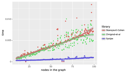
Figure 3: Speed comparison of Non-Projective Spanning Tree libraries.

A.3 Comparison of Maximum Projective Spanning Tree Algorithms

Eisner’s algorithm is virtually the only projective parsing algorithm actively used, if we do not count the transition based parsers. We have found that replacing Eisner’s algorithm with Kuhlmann et al. (2011) tabulation of arc-hybrid algorithm can provide large speed gains both on CPU and GPU. See Figure 4. In this implementation graph size does not make a big difference because it is implemented in a vectorized way so most operations are parallelized.

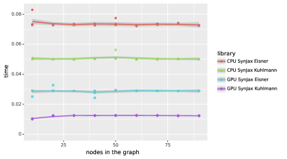
Figure 4: Speed comparison of Projective Maximum Spanning Tree algorithms.

References

- Abdel-Hamid et al. (2013) Ossama Abdel-Hamid, Li Deng, Dong Yu, and Hui Jiang. 2013. Deep segmental neural networks for speech recognition. In Interspeech, volume 36.
- Aziz (2015) Wilker Aziz. 2015. Grasp: Randomised Semiring Parsing. Prague Bulletin of Mathematical Linguistics, 104:51–62.
- Babuschkin et al. (2020) Igor Babuschkin, Kate Baumli, Alison Bell, Surya Bhupatiraju, Jake Bruce, Peter Buchlovsky, David Budden, Trevor Cai, Aidan Clark, Ivo Danihelka, Antoine Dedieu, Claudio Fantacci, Jonathan Godwin, Chris Jones, Ross Hemsley, Tom Hennigan, Matteo Hessel, Shaobo Hou, Steven Kapturowski, Thomas Keck, Iurii Kemaev, Michael King, Markus Kunesch, Lena Martens, Hamza Merzic, Vladimir Mikulik, Tamara Norman, George Papamakarios, John Quan, Roman Ring, Francisco Ruiz, Alvaro Sanchez, Laurent Sartran, Rosalia Schneider, Eren Sezener, Stephen Spencer, Srivatsan Srinivasan, Miloš Stanojević, Wojciech Stokowiec, Luyu Wang, Guangyao Zhou, and Fabio Viola. 2020. The DeepMind JAX Ecosystem.
- Bastings et al. (2019) Jasmijn Bastings, Wilker Aziz, and Ivan Titov. 2019. Interpretable neural predictions with differentiable binary variables. In Proceedings of the 57th Annual Meeting of the Association for Computational Linguistics, pages 2963–2977, Florence, Italy. Association for Computational Linguistics.
- Bastings et al. (2017) Jasmijn Bastings, Ivan Titov, Wilker Aziz, Diego Marcheggiani, and Khalil Sima’an. 2017. Graph convolutional encoders for syntax-aware neural machine translation. In Proceedings of the 2017 Conference on Empirical Methods in Natural Language Processing, pages 1957–1967, Copenhagen, Denmark. Association for Computational Linguistics.
- Bisk and Tran (2018) Yonatan Bisk and Ke Tran. 2018. Inducing grammars with and for neural machine translation. In Proceedings of the 2nd Workshop on Neural Machine Translation and Generation, pages 25–35, Melbourne, Australia. Association for Computational Linguistics.
- Chang et al. (2023) Oscar Chang, Dongseong Hwang, and Olivier Siohan. 2023. Revisiting the Entropy Semiring for Neural Speech Recognition. In The Eleventh International Conference on Learning Representations.
- Chang et al. (2022) Peter Chang, Giles Harper-Donnelly, Aleyna Kara, Xinglong Li, Scott Linderman, and Kevin Murphy. 2022. Dynamax.
- Choe and Charniak (2016) Do Kook Choe and Eugene Charniak. 2016. Parsing as language modeling. In Proceedings of the 2016 Conference on Empirical Methods in Natural Language Processing, pages 2331–2336, Austin, Texas. Association for Computational Linguistics.
- Cohen et al. (2013) Shay B. Cohen, Giorgio Satta, and Michael Collins. 2013. Approximate PCFG parsing using tensor decomposition. In Proceedings of the 2013 Conference of the North American Chapter of the Association for Computational Linguistics: Human Language Technologies, pages 487–496, Atlanta, Georgia. Association for Computational Linguistics.
- Colbourn et al. (1996) Charles J. Colbourn, Wendy J. Myrvold, and Eugene Neufeld. 1996. Two Algorithms for Unranking Arborescences. Journal of Algorithms, 20(2):268–281.
- Corro and Titov (2019) Caio Corro and Ivan Titov. 2019. Differentiable Perturb-and-Parse: Semi-Supervised Parsing with a Structured Variational Autoencoder. In International Conference on Learning Representations.
- Cortes et al. (2008) Corinna Cortes, Mehryar Mohri, Ashish Rastogi, and Michael Riley. 2008. On the computation of the relative entropy of probabilistic automata. International Journal of Foundations of Computer Science, 19(01):219–242.
- Crouse (2016) David F Crouse. 2016. On implementing 2D rectangular assignment algorithms. IEEE Transactions on Aerospace and Electronic Systems, 52(4):1679–1696.
- Cuturi and Blondel (2017) Marco Cuturi and Mathieu Blondel. 2017. Soft-DTW: A Differentiable Loss Function for Time-Series. In Proceedings of the 34th International Conference on Machine Learning - Volume 70, ICML’17, page 894–903. JMLR.org.
- Darwiche (2003) Adnan Darwiche. 2003. A Differential Approach to Inference in Bayesian Networks. J. ACM, 50(3):280–305.
- Day et al. (2007) Nathan Day, Andrew Hemmaplardh, Robert E. Thurman, John A. Stamatoyannopoulos, and William S. Noble. 2007. Unsupervised segmentation of continuous genomic data. Bioinformatics, 23(11):1424–1426.
- Dillon et al. (2017) Joshua V. Dillon, Ian Langmore, Dustin Tran, Eugene Brevdo, Srinivas Vasudevan, Dave Moore, Brian Patton, Alex Alemi, Matt Hoffman, and Rif A. Saurous. 2017. TensorFlow Distributions.
- Dyer et al. (2016) Chris Dyer, Adhiguna Kuncoro, Miguel Ballesteros, and Noah A. Smith. 2016. Recurrent neural network grammars. In Proceedings of the 2016 Conference of the North American Chapter of the Association for Computational Linguistics: Human Language Technologies, pages 199–209, San Diego, California. Association for Computational Linguistics.
- Eisner (1996) Jason Eisner. 1996. Three new probabilistic models for dependency parsing: An exploration. In COLING 1996 Volume 1: The 16th International Conference on Computational Linguistics.
- Eisner (2002) Jason Eisner. 2002. Parameter estimation for probabilistic finite-state transducers. In Proceedings of the 40th Annual Meeting of the Association for Computational Linguistics, pages 1–8, Philadelphia, Pennsylvania, USA. Association for Computational Linguistics.
- Eisner (2016) Jason Eisner. 2016. Inside-Outside and Forward-Backward Algorithms Are Just Backprop (tutorial paper). In Proceedings of the Workshop on Structured Prediction for NLP, pages 1–17, Austin, TX. Association for Computational Linguistics.
- Fu et al. (2020) Yao Fu, Chuanqi Tan, Bin Bi, Mosha Chen, Yansong Feng, and Alexander M. Rush. 2020. Latent template induction with gumbel-crfs. In Proceedings of the 34th International Conference on Neural Information Processing Systems, NIPS’20, Red Hook, NY, USA. Curran Associates Inc.
- Goodman (1999) Joshua Goodman. 1999. Semiring Parsing. Computational Linguistics, 25(4):573–606.
- Graves et al. (2006) Alex Graves, Santiago Fernández, Faustino Gomez, and Jürgen Schmidhuber. 2006. Connectionist Temporal Classification: Labelling Unsegmented Sequence Data with Recurrent Neural Networks. In Proceedings of the 23rd International Conference on Machine Learning, pages 369–376.
- Griewank (1992) Andreas Griewank. 1992. Achieving logarithmic growth of temporal and spatial complexity in reverse automatic differentiation. Optimization Methods and Software, 1(1):35–54.
- Hannun (2017) Awni Hannun. 2017. Sequence Modeling with CTC. Distill. https://distill.pub/2017/ctc.
- Havrylov et al. (2019) Serhii Havrylov, Germán Kruszewski, and Armand Joulin. 2019. Cooperative learning of disjoint syntax and semantics. In Proceedings of the 2019 Conference of the North American Chapter of the Association for Computational Linguistics: Human Language Technologies, Volume 1 (Long and Short Papers), pages 1118–1128, Minneapolis, Minnesota. Association for Computational Linguistics.
- Hockenmaier et al. (2007) Julia Hockenmaier, Aravind K Joshi, and Ken A Dill. 2007. Routes are trees: the parsing perspective on protein folding. Proteins: Structure, Function, and Bioinformatics, 66(1):1–15.
- Huang et al. (2019) Liang Huang, He Zhang, Dezhong Deng, Kai Zhao, Kaibo Liu, David A Hendrix, and David H Mathews. 2019. LinearFold: linear-time approximate RNA folding by 5’-to-3’ dynamic programming and beam search. Bioinformatics, 35(14):i295–i304.
- Hwa (2000) Rebecca Hwa. 2000. Sample selection for statistical grammar induction. In 2000 Joint SIGDAT Conference on Empirical Methods in Natural Language Processing and Very Large Corpora, pages 45–52, Hong Kong, China. Association for Computational Linguistics.
- Kidger and Garcia (2021) Patrick Kidger and Cristian Garcia. 2021. Equinox: neural networks in JAX via callable PyTrees and filtered transformations.
- Kim et al. (2017) Yoon Kim, Carl Denton, Luong Hoang, and Alexander M. Rush. 2017. Structured attention networks. In International Conference on Learning Representations.
- Kim et al. (2019) Yoon Kim, Chris Dyer, and Alexander Rush. 2019. Compound probabilistic context-free grammars for grammar induction. In Proceedings of the 57th Annual Meeting of the Association for Computational Linguistics, pages 2369–2385, Florence, Italy. Association for Computational Linguistics.
- Kitaev et al. (2019) Nikita Kitaev, Steven Cao, and Dan Klein. 2019. Multilingual constituency parsing with self-attention and pre-training. In Proceedings of the 57th Annual Meeting of the Association for Computational Linguistics, pages 3499–3505, Florence, Italy. Association for Computational Linguistics.
- Koo et al. (2007) Terry Koo, Amir Globerson, Xavier Carreras, and Michael Collins. 2007. Structured Prediction Models via the Matrix-Tree Theorem. In Proceedings of the 2007 Joint Conference on Empirical Methods in Natural Language Processing and Computational Natural Language Learning (EMNLP-CoNLL), pages 141–150, Prague, Czech Republic. Association for Computational Linguistics.
- Kuhlmann et al. (2011) Marco Kuhlmann, Carlos Gómez-Rodríguez, and Giorgio Satta. 2011. Dynamic programming algorithms for transition-based dependency parsers. In Proceedings of the 49th Annual Meeting of the Association for Computational Linguistics: Human Language Technologies, pages 673–682, Portland, Oregon, USA. Association for Computational Linguistics.
- Lafferty et al. (2001) John D. Lafferty, Andrew McCallum, and Fernando C. N. Pereira. 2001. Conditional Random Fields: Probabilistic Models for Segmenting and Labeling Sequence Data. In Proceedings of the Eighteenth International Conference on Machine Learning, ICML ’01, page 282–289, San Francisco, CA, USA. Morgan Kaufmann Publishers Inc.
- Lam et al. (2015) Siu Kwan Lam, Antoine Pitrou, and Stanley Seibert. 2015. Numba: A llvm-based python jit compiler. In Proceedings of the Second Workshop on the LLVM Compiler Infrastructure in HPC, LLVM ’15, New York, NY, USA. Association for Computing Machinery.
- Li and Eisner (2009) Zhifei Li and Jason Eisner. 2009. First- and second-order expectation semirings with applications to minimum-risk training on translation forests. In Proceedings of the 2009 Conference on Empirical Methods in Natural Language Processing, pages 40–51, Singapore. Association for Computational Linguistics.
- Lu et al. (2016) Liang Lu, Lingpeng Kong, Chris Dyer, Noah A Smith, and Steve Renals. 2016. Segmental recurrent neural networks for end-to-end speech recognition. In Proceedings of the 17th Annual Conference of the International Speech Communication Association (INTERSPEECH 2016).
- Lyu and Titov (2018) Chunchuan Lyu and Ivan Titov. 2018. AMR parsing as graph prediction with latent alignment. In Proceedings of the 56th Annual Meeting of the Association for Computational Linguistics (Volume 1: Long Papers), pages 397–407, Melbourne, Australia. Association for Computational Linguistics.
- Ma and Hovy (2016) Xuezhe Ma and Eduard Hovy. 2016. End-to-end sequence labeling via bi-directional LSTM-CNNs-CRF. In Proceedings of the 54th Annual Meeting of the Association for Computational Linguistics (Volume 1: Long Papers), pages 1064–1074, Berlin, Germany. Association for Computational Linguistics.
- Martins et al. (2010) André Martins, Noah Smith, Eric Xing, Pedro Aguiar, and Mário Figueiredo. 2010. Turbo parsers: Dependency parsing by approximate variational inference. In Proceedings of the 2010 Conference on Empirical Methods in Natural Language Processing, pages 34–44, Cambridge, MA. Association for Computational Linguistics.
- Mena et al. (2018) Gonzalo Mena, David Belanger, Scott Linderman, and Jasper Snoek. 2018. Learning Latent Permutations with Gumbel-Sinkhorn Networks. In International Conference on Learning Representations.
- Mensch and Blondel (2018) Arthur Mensch and Mathieu Blondel. 2018. Differentiable dynamic programming for structured prediction and attention. In Proceedings of the 35th International Conference on Machine Learning, volume 80 of Proceedings of Machine Learning Research, pages 3462–3471. PMLR.
- Mihaylova et al. (2020) Tsvetomila Mihaylova, Vlad Niculae, and André F. T. Martins. 2020. Understanding the Mechanics of SPIGOT: Surrogate Gradients for Latent Structure Learning. In Proceedings of the 2020 Conference on Empirical Methods in Natural Language Processing (EMNLP), pages 2186–2202, Online. Association for Computational Linguistics.
- Murphy (2012) Kevin P. Murphy. 2012. Machine Learning: A Probabilistic Perspective. Adaptive Computation and Machine Learning Series. The MIT Press.
- Nădejde et al. (2017) Maria Nădejde, Siva Reddy, Rico Sennrich, Tomasz Dwojak, Marcin Junczys-Dowmunt, Philipp Koehn, and Alexandra Birch. 2017. Predicting target language CCG supertags improves neural machine translation. In Proceedings of the Second Conference on Machine Translation, pages 68–79, Copenhagen, Denmark. Association for Computational Linguistics.
- Needleman and Wunsch (1970) S. B. Needleman and C. D. Wunsch. 1970. A general method applicable to the search for similarities in the amino acid sequence of two proteins. Journal of Molecular Biology, 48:443–453.
- Niepert et al. (2021) Mathias Niepert, Pasquale Minervini, and Luca Franceschi. 2021. Implicit mle: backpropagating through discrete exponential family distributions. Advances in Neural Information Processing Systems, 34:14567–14579.
- Paulus et al. (2020) Max Paulus, Dami Choi, Daniel Tarlow, Andreas Krause, and Chris J Maddison. 2020. Gradient estimation with stochastic softmax tricks. In Advances in Neural Information Processing Systems, volume 33, pages 5691–5704. Curran Associates, Inc.
- Peharz et al. (2020) Robert Peharz, Steven Lang, Antonio Vergari, Karl Stelzner, Alejandro Molina, Martin Trapp, Guy Van Den Broeck, Kristian Kersting, and Zoubin Ghahramani. 2020. Einsum Networks: Fast and Scalable Learning of Tractable Probabilistic Circuits. In Proceedings of the 37th International Conference on Machine Learning, ICML’20. JMLR.org.
- Phan et al. (2019) Du Phan, Neeraj Pradhan, and Martin Jankowiak. 2019. Composable Effects for Flexible and Accelerated Probabilistic Programming in NumPyro. In Program Transformations for ML Workshop at NeurIPS 2019.
- Pogančić et al. (2020) Marin Vlastelica Pogančić, Anselm Paulus, Vit Musil, Georg Martius, and Michal Rolinek. 2020. Differentiation of Blackbox Combinatorial Solvers. In International Conference on Learning Representations.
- Rabiner (1990) Lawrence R. Rabiner. 1990. A tutorial on hidden markov models and selected applications in speech recognition. In Readings in Speech Recognition, pages 267–296. Elsevier.
- Rush (2020) Alexander Rush. 2020. Torch-Struct: Deep Structured Prediction Library. In Proceedings of the 58th Annual Meeting of the Association for Computational Linguistics: System Demonstrations, pages 335–342, Online. Association for Computational Linguistics.
- Sakakibara et al. (1994) Sakakibara, Underwood, Mian, and Haussler. 1994. Stochastic Context-Free Grammars for Modeling RNA. In 1994 Proceedings of the Twenty-Seventh Hawaii International Conference on System Sciences, volume 5, pages 284–293. IEEE.
- Sarawagi and Cohen (2004) Sunita Sarawagi and William W Cohen. 2004. Semi-markov conditional random fields for information extraction. In Advances in Neural Information Processing Systems, volume 17. MIT Press.
- Sartran et al. (2022) Laurent Sartran, Samuel Barrett, Adhiguna Kuncoro, Miloš Stanojević, Phil Blunsom, and Chris Dyer. 2022. Transformer Grammars: Augmenting Transformer Language Models with Syntactic Inductive Biases at Scale. Transactions of the Association for Computational Linguistics, 10:1423–1439.
- Smith and Smith (2007) David A. Smith and Noah A. Smith. 2007. Probabilistic Models of Nonprojective Dependency Trees. In Proceedings of the 2007 Joint Conference on Empirical Methods in Natural Language Processing and Computational Natural Language Learning (EMNLP-CoNLL), pages 132–140, Prague, Czech Republic. Association for Computational Linguistics.
- Stanojević (2022) Miloš Stanojević. 2022. Unbiased and efficient sampling of dependency trees. In Proceedings of the 2022 Conference on Empirical Methods in Natural Language Processing, pages 1691–1706, Abu Dhabi, United Arab Emirates. Association for Computational Linguistics.
- Stanojević and Cohen (2021) Miloš Stanojević and Shay B. Cohen. 2021. A Root of a Problem: Optimizing Single-Root Dependency Parsing. In Proceedings of the 2021 Conference on Empirical Methods in Natural Language Processing, pages 10540–10557, Online and Punta Cana, Dominican Republic. Association for Computational Linguistics.
- Stern et al. (2017) Mitchell Stern, Jacob Andreas, and Dan Klein. 2017. A minimal span-based neural constituency parser. In Proceedings of the 55th Annual Meeting of the Association for Computational Linguistics (Volume 1: Long Papers), pages 818–827, Vancouver, Canada. Association for Computational Linguistics.
- Sutton and McCallum (2007) Charles Sutton and Andrew McCallum. 2007. An Introduction to Conditional Random Fields for Relational Learning. Introduction to statistical relational learning, page 93.
- Särkkä and García-Fernández (2021) Simo Särkkä and Ángel F. García-Fernández. 2021. Temporal Parallelization of Bayesian Smoothers. IEEE Transactions on Automatic Control, 66(1):299–306.
- Tarjan (1977) R. E. Tarjan. 1977. Finding optimum branchings. Networks, 7(1):25–35.
- Tran et al. (2016) Ke M. Tran, Yonatan Bisk, Ashish Vaswani, Daniel Marcu, and Kevin Knight. 2016. Unsupervised neural hidden Markov models. In Proceedings of the Workshop on Structured Prediction for NLP, pages 63–71, Austin, TX. Association for Computational Linguistics.
- Tutte (1984) W. T. Tutte. 1984. Graph Theory, volume 21 of Encyclopedia of Mathematics and Its Applications. Addison-Wesley, Menlo Park, CA.
- Valiant (1979) L.G. Valiant. 1979. The complexity of computing the permanent. Theoretical Computer Science, 8(2):189–201.
- Virtanen et al. (2020) Pauli Virtanen, Ralf Gommers, Travis E. Oliphant, Matt Haberland, Tyler Reddy, David Cournapeau, Evgeni Burovski, Pearu Peterson, Warren Weckesser, Jonathan Bright, Stéfan J. van der Walt, Matthew Brett, Joshua Wilson, K. Jarrod Millman, Nikolay Mayorov, Andrew R. J. Nelson, Eric Jones, Robert Kern, Eric Larson, C J Carey, İlhan Polat, Yu Feng, Eric W. Moore, Jake VanderPlas, Denis Laxalde, Josef Perktold, Robert Cimrman, Ian Henriksen, E. A. Quintero, Charles R. Harris, Anne M. Archibald, Antônio H. Ribeiro, Fabian Pedregosa, Paul van Mulbregt, and SciPy 1.0 Contributors. 2020. SciPy 1.0: Fundamental Algorithms for Scientific Computing in Python. Nature Methods, 17:261–272.
- Wang and Xu (2011) Zhiyong Wang and Jinbo Xu. 2011. A conditional random fields method for RNA sequence–structure relationship modeling and conformation sampling. Bioinformatics, 27(13):i102–i110.
- Williams (1992) Ronald J. Williams. 1992. Simple statistical gradient-following algorithms for connectionist reinforcement learning. Mach. Learn., 8(3–4):229–256.
- Wilson (1996) David Bruce Wilson. 1996. Generating Random Spanning Trees More Quickly than the Cover Time. In Proceedings of the Twenty-Eighth Annual ACM Symposium on Theory of Computing, STOC ’96, page 296–303, New York, NY, USA. Association for Computing Machinery.
- Yang et al. (2022) Songlin Yang, Wei Liu, and Kewei Tu. 2022. Dynamic programming in rank space: Scaling structured inference with low-rank HMMs and PCFGs. In Proceedings of the 2022 Conference of the North American Chapter of the Association for Computational Linguistics: Human Language Technologies, pages 4797–4809, Seattle, United States. Association for Computational Linguistics.
- Zhou et al. (2023) Guangyao Zhou, Antoine Dedieu, Nishanth Kumar, Wolfgang Lehrach, Miguel Lázaro-Gredilla, Shrinu Kushagra, and Dileep George. 2023. Pgmax: Factor graphs for discrete probabilistic graphical models and loopy belief propagation in jax.
- Zmigrod et al. (2020) Ran Zmigrod, Tim Vieira, and Ryan Cotterell. 2020. Please Mind the Root: Decoding Arborescences for Dependency Parsing. In Proceedings of the 2020 Conference on Empirical Methods in Natural Language Processing (EMNLP), pages 4809–4819, Online. Association for Computational Linguistics.
- Zmigrod et al. (2021) Ran Zmigrod, Tim Vieira, and Ryan Cotterell. 2021. Efficient Computation of Expectations under Spanning Tree Distributions. 9:675–690.