FLIQS: One-Shot Mixed-Precision Floating-Point
and Integer Quantization Search

Abstract

Quantization has become a mainstream compression technique for reducing model size, computational requirements, and energy consumption for modern deep neural networks (DNNs). With the improved numerical support in recent hardware, including multiple variants of integer and floating point, mixed-precision quantization has become necessary to achieve high-quality results with low model cost. Prior mixed-precision quantization methods have performed a post-training quantization search, which compromises on accuracy, or a differentiable quantization search, which leads to high memory usage from branching. Therefore, we propose the first one-shot mixed-precision quantization search that eliminates the need for retraining in both integer and low-precision floating point models. We evaluate our floating-point and integer quantization search (FLIQS) on multiple convolutional networks and vision transformer models to discover Pareto-optimal models. Our approach discovers models that improve upon uniform precision, manual mixed-precision, and recent integer quantization search methods. With the proposed integer quantization search, we increase the accuracy of ResNet-18 on ImageNet by 1.31% points and ResNet-50 by 0.90% points with equivalent model cost over previous methods. Additionally, for the first time, we explore a novel mixed-precision floating-point search and improve MobileNetV2 by up to 0.98% points compared to prior state-of-the-art FP8 models. Finally, we extend FLIQS to simultaneously search a joint quantization and neural architecture space and improve the ImageNet accuracy by 2.69% points with similar model cost on a MobileNetV2 search space.

1 Introduction

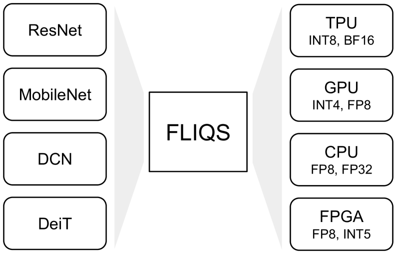
(a)

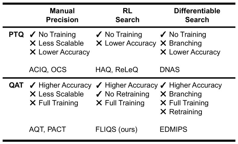
(b)

Figure 1: FLIQS – The explosion of model architectures, numerical support, and deployment platforms requires automated methods for searching model configurations to utilize platform-specific numerical formats. We establish FLIQS as the first one-shot quantization and neural architecture search framework without retraining for searching for mixed-precision integer and floating point formats. Compared to prior work, it establishes a more scalable and memory-efficient approach by avoiding additional branching during the search.

In recent years, deep neural networks (DNNs) have attained state-of-the-art results on a wide range of tasks including image classification, speech recognition, image and speech generation, and recommendation systems. Each model iteration typically enhances quality but also tends to increase computation, memory usage, and power consumption. These increases limit DNN adoption in resource-constrained edge devices, worsen their latency across platforms, and expand their carbon footprint, especially within cloud systems. DNN quantization to low-precision formats has become the standard method for reducing model storage size, memory bandwidth, and complexity of MAC operations Gholami et al. (2021); Hao et al. (2021). These formats include both integer and low-precision floating-point, which has recently gained attention as a flexible alternative to integer formats.

At the same time, DNN accelerators have become more diverse and now support a wide range of numerical formats. For example, the Google TPUv3 supports FP32, BF16, FP16, and INT8 Jouppi et al. (2020), while the latest NVIDIA Hopper architecture supports FP32, BF16, FP8, and INT8 Nvidia (2020). Furthermore, reprogrammable systems such as FPGA devices allow arbitrary precision arithmetic such as INT5, FP11, FP9, or FP8 for more granular accuracy-performance trade-offs Abdelfattah et al. (2018). While these devices enable mixed-precision quantization, where layers take on different formats within the same model, it remains a challenge to optimally assign per-layer formats since layers exhibit different quantization characteristics. In simple cases, this assignment can be performed manually, yet with the explosion of DNN architectures and accelerator designs, automated methods are more reliable, scalable, and reproducible for achieving high accuracy and performance.

In this paper, we introduce FLoating-Point and Integer Quantization Search (FLIQS) to automate mixed-precision floating-point and integer quantization and automatically assign per-layer formats. In addition, FLIQS can jointly optimize for quantization formats and neural architecture to intelligently allocate compute across the kernel, channel, and bitwidth dimensions. FLIQS is a one-shot search based on reinforcement learning (RL) and unlike expensive multi-trial searches, it avoids training separate models for each configuration, leading to overall reduced search overhead. Furthermore, as the search takes place during training, FLIQS can achieve higher accuracies than post-training quantization (PTQ) searches. Coupled with additional entropy regularization, the final model can be deployed without the need for further retraining or fine-tuning. As shown in Figure 1(a), FLIQS accelerates the process of adapting legacy models to new hardware, co-designing models and accelerators, and finding Pareto-optimal models on current hardware systems. We summarize our contributions as follows:

1. Introduce and open-source the first one-shot quantization search without retraining through the addition of a new cosine entropy regularization schedule;

2. Demonstrate state-of-the-art results for integer and low-precision floating-point quantization search across a range of convolutional and transformer networks;

3. Perform the largest comparison of integer and floating-point mixed-precision networks;

4. Conduct the first study of quantization and neural architecture search on low-precision floating-point networks and establish recommendations for allocating compute across bitwidth and neural architectural dimensions.

2 Related Work

Low-Precision Floating Point: Low-precision floating point is being discussed as the next generation format for DNN training and inference. Micikevicius et al. (2022). Companies, including AMD, Intel, NVIDIA, and Qualcomm, have recently agreed to adopt 8-bit floating-point (FP8) in future deep learning systems. Within these formats, recent studies generally focus on two variants: E5M2 and E4M3, where E represents the number of exponent bits and M is the number of mantissa bits. For example, HFP8 suggests using E4M3 for the forward pass and E5M2 for backpropagation Sun et al. (2019). Building upon these uniform precision works  Sun et al. (2019); Mellempudi et al. (2019); Kuzmin et al. (2022); Huang et al. (2021); Lee et al. (2022), FLIQS proposes an automated approach for finding mixed-precision floating-point networks, compares these to mixed-precision integer networks with similar cost, and performs a joint floating-point quantization and neural architecture search.

Quantization Search: Prior work has explored mixed-precision integer quantization searches, as shown in Figure 1(b). For instance, HAQ Wang et al. (2019) and ReLeQ Elthakeb et al. (2020) both perform PTQ quantization searches that utilize RL to allocate bitwidths based on the model accuracy and cost estimates. In addition, the HAWQ series of works further develops these PTQ searches, using the Hessian spectrum to determine layer sensitivities and constrained ILP formulations to find optimal bitwidth configurations Dong et al. (2019, 2020); Yao et al. (2021). However, being PTQ-based, these methods cannot take advantage of the higher accuracy and more accurate feedback provided by quantization-aware training (QAT) during the search.

Other efforts combine QAT with neural architecture search (NAS), using super-networks and differentiable NAS Wu et al. (2018); Zhao et al. (2021); Bai et al. (2021); Elthakeb et al. (2020). For instance, EDMIPS creates branches for each bitwidth, forms a linear combination of them, and then alternates training the layer weights and the branch weights Cai and Vasconcelos (2020). These differentiable searches often have simpler formulations since the layer and branch weights are unified and trained together with gradient descent. However, because they duplicate the weights and activations multiple times, they incur higher memory and computational costs compared to RL-based methods. In addition, both PTQ and QAT prior works require additional retraining steps on the model after the search, while FLIQS directly serves the final model without fine-tuning.

Quantization Neural Architecture Search (QNAS): In addition, prior work has explored joint search spaces with quantization formats and neural architecture Fu et al. (2021); Gong et al. (2019); Wang et al. (2020). For example, APQ uses knowledge distillation from a full-precision accuracy predictor to optimize neural architecture, quantization formats, and pruning policies Wang et al. (2020). FLIQS expands on this line of work by jointly searching quantization formats and neural architecture and highlights trends for allocating compute across this joint search space for high accuracy and performance.

3 FLIQS Framework

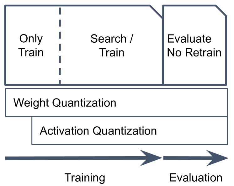
(a)

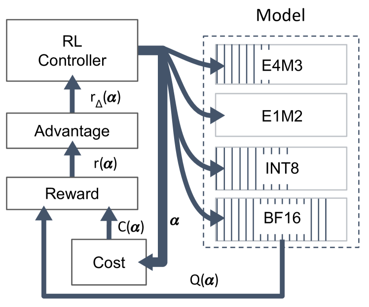
(b)

Figure 2: FLIQS Overview – (a) FLIQS begins with pure training to allow the reward signal to stabilize before updating its policy. The activation quantization is delayed to allow the activation statistics to stabalize. (b) The RL controller proposes per-layer formats and architectural decisions during training, indicated by the numerical format variable $\boldsymbol{\alpha}$. The vertical grid lines represent per-layer channel masks that dynamically zero out channels during training to simulate different channel widths. The model applies $\boldsymbol{\alpha}$ to each layer and produces a quality signal $Q(\boldsymbol{\alpha})$, which is combined with the model cost $C(\boldsymbol{\alpha})$ to produce the reward $r(\boldsymbol{\alpha})$ and reward advantage $r_{\Delta}(\boldsymbol{\alpha})$.

In Figure 2(a), FLIQS employs an RL controller to sample per-layer formats and channel widths during training, collectively referred to as the architecture. This section focuses on this QNAS search space, while simpler and more complex searches are explored in later sections. Initially, the model trains without search, and the architecture is sampled uniformly at random to avoid overfitting to a single option. Next, at each training step, the controller proposes a new architecture and applies it to the model. The model then performs a standard forward and backward pass on the training data to produce the model gradients and a forward pass on the validation data to produce a quality signal for the controller. This quality signal is combined with the model cost in Figure 2(b) to produce a reward and reward advantage, which the controller then uses to update its policy. After the search and training finish, the model is directly used for inference without additional fine-tuning or retraining.

Challenges: This approach introduces a unique set of challenges. First, the search may interfere with the original model training process, since modifying the architecture shifts the weight and activation distributions during training. In addition, one-shot search needs to evaluate the quality signal of different architectures on different batches of training data to avoid lengthening the training process. This introduces noise into the reward signal since different batches may have significantly different quality. This noise is further compounded by the natural increase in the quality signal throughout training. Furthermore, the controller and policy model must be efficient enough to be embedded within the training graph to not significantly increase the training time. These challenges are addressed in the following sections.

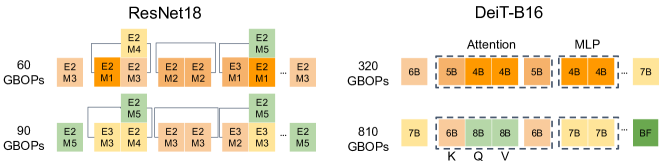
Figure 3: FLIQS Examples – In these quantization search examples, FLIQS allocates more precision to the first and last layers and the small pointwise convolutions of ResNet-18, and to the attention block within DeiT-B16. More configurations are listed in Appendix A.1.

Cost and Reward Function: FLIQS uses the quadratic cost model, bit operations (BOPs), as described in Equation 1 where $b(\alpha)$ is the total bitwidth of the current layer architecture $\alpha$ and $MAC_{l}(\alpha)$ represents the number of multiply-accumulates (MACs) in layer $l$. Quadratic cost models, which predict power and area, are particularly useful in model-accelerator co-design where multipliers dominate resources and scale quadratically in power and area Zhang et al. (2022).

$$C_{l}(\alpha)=b(\alpha)^{2}{MAC_{l}(\alpha)}$$ (1)

$$r(\boldsymbol{\alpha})=Q(\boldsymbol{\alpha})+\gamma|\frac{\sum_{l}{C_{l}(\alpha)}}{C_{T}}-1|$$ (2)

This model cost is combined with the quality signal in the absolute reward function shown in Equation 2 Bender et al. (2020). The absolute reward function includes a cost target $C_{T}$ that provides the user control over the accuracy-performance trade off. More restrictive targets tend to result in less compute-intensive models (as shown in Figure 3), which often have lower accuracy. This resultant cost term is combined with the model quality using the cost scalar $\gamma$, which balances the importance of performance and quality.

RL Controller: The RL controller learns a policy $\pi_{l}(\alpha)$ for each layer $l$ that represents a probability distribution over each layer architecture $\alpha$. At each training step, the controller samples and applies a new layer architecture $\alpha_{l}\sim\pi_{l}(\alpha)$. The channel widths are efficiently searched by applying channel masks, which dynamically zero out channels and reuse the underlying weights during training. This policy $\pi_{l}(\alpha)$ is parameterized by $\theta_{l,\alpha}$, where $\theta_{l,\alpha}$ represents the logit for the $\alpha^{th}$ decision in the $l^{th}$ layer. These logits are then passed through a softmax layer to produce the policy probability distribution.

$$\pi_{l}(\alpha)=\frac{\exp(\theta_{l,\alpha})}{\sum_{j}\exp(\theta_{l,j})}$$ (3)

After sampling and assigning the model architecture, $\boldsymbol{\alpha}$, the reward $r(\boldsymbol{\alpha})$ is calculated according to Equation 2. However, since the reward depends on the quality signal, which increases throughout training, the difference between the running average of previous rewards, $\bar{r}(\boldsymbol{\alpha})$, and the current reward is used instead: $r_{\Delta}(\boldsymbol{\alpha})=\bar{r}(\boldsymbol{\alpha})-r(\boldsymbol{\alpha})$. Then, the REINFORCE algorithm Williams (1992) is used to update the policy $\pi_{l}(\alpha)$ by performing gradient descent on the policy loss, $\mathcal{L}_{\theta}$:

$$\mathcal{L}_{\theta} =-r_{\Delta}(\boldsymbol{\alpha})\sum_{l}{\log{(\alpha_{l}\sim\pi_{l}(\alpha)})}$$ (4)

$$\theta \leftarrow\theta+\eta\nabla_{\theta}\mathcal{L}_{\theta}$$ (5)

where $\eta$ is the RL learning rate. This procedure is chosen due to its low complexity, and it helps address the performance concerns with one-shot searches. A performance comparison of one-shot search techniques is shown in Appendix A.6. Other reinforcement learning methods, such as PPO, and more sophisticated policy models, such as multi-layer perceptron models, offered no quality improvements while being more costly to compute.

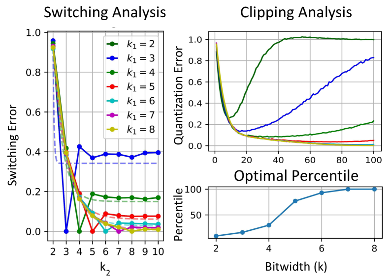
(a) Switching and Clipping

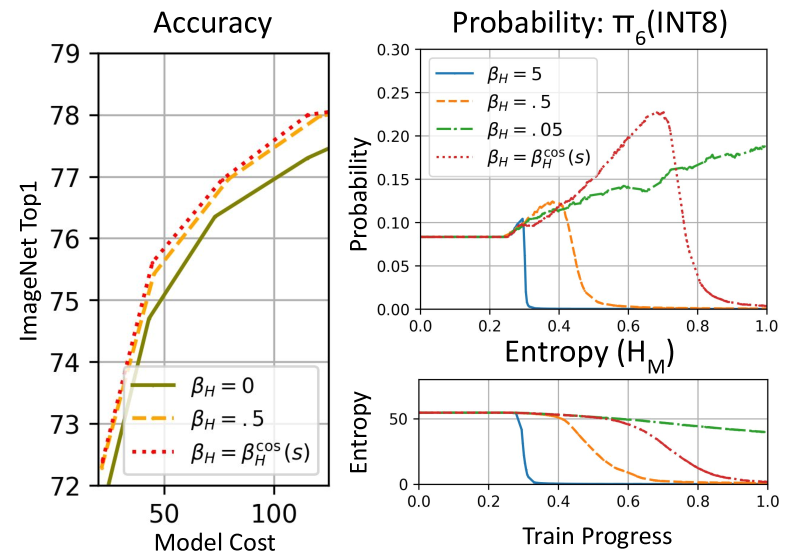
(b) Entropy Regularization

Figure 4: FLIQS Analysis – (a) The switching error between $k_{1}$ and $k_{2}$ bitwidths grows relatively large when either bitwidth is small, which can potentially affect the model convergence. The dashed lines represent the best-fit exponential curves. In addition, the optimal clipping threshold depends on the current bitwidth, which motivates swapping thresholds during the quantization search. Setup details for this analysis are located in Appendix A.8. (b) Accuracy improves for higher entropy regularization, and the entropy regularization affects the policy convergence, where $H_{M}$ is the total model entropy and $\pi_{6}$(INT8) is the probability of sampling INT8 from the sixth layer of ResNet50. $\beta_{H}^{\cos}$ achieves the same final convergence as higher regularization, which promotes stable training at the end of the search, with the same high entropy in the early stages as lower regularization.

Format Search Space: For pure quantization search, this work evaluates FLIQS on two search spaces: FLIQS-S and FLIQS-L. FLIQS-S includes the standard power-of-two formats, while FLIQS-L includes a larger set of formats between four and eight bits. For floating point, FLIQS-L includes 16 formats, which to our knowledge is the largest quantization search performed. Full details of the quantization search spaces can be found in Appendix A.5.

Quantization and Weight Sharing: Each layer in FLIQS searches has a single set of full-precision model weights, which are dynamically quantized and masked at each step based on the architecture sampled by the RL controller. A detailed description of the quantization procedure can be found in Appendix A.2. This approach differs from other works like DNAS Wu et al. (2018) and EDMIPS Cai and Vasconcelos (2020), which use branched super-networks that allocate each numerical format its own set of weights and activations. These additional branches can become prohibitively large due to the additional weight memory and gradient buffers especially for larger search spaces, such as the floating-point FLIQS-L space.

Switchable Clipping: FLIQS introduces a switchable clipping threshold (formally defined in Appendix A.2) based on the current format selection. This is necessary since smaller bitwidths require more aggressive clipping, and vice versa, as shown in Figure 4(a). These clipping thresholds can either be pre-computed with synthetic data, or computed during the first phase of the search with real data. In general, pre-computing the thresholds leads to high-quality results with less complexity, and it is used for the experimental sections below.

4 FLIQS Analysis

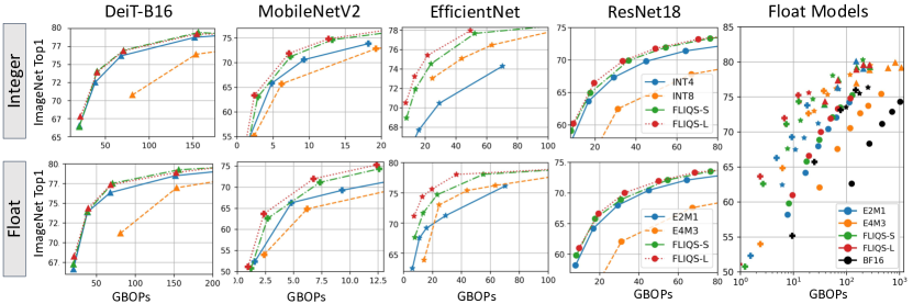
Figure 5: ImageNet FLIQS Quantization Search – FLIQS reaches higher accuracies at lower costs, and in general FLIQS-L achieves higher accuracies. Models are evaluated at multiple widths ranging .25$\times$ to 2$\times$ of their original channel width to generate each data point, except for EfficientNet where variants B[0,4] are used. All of the corresponding table data and the additional Pareto curves for InceptionV3 and ResNet50 are located in Appendix A.14.

Switching Error: The primary challenge for FLIQS is minimizing the effect of the search on the model training. Within a pure quantization search, this effect can be formalized by introducing the switching error. Consider the standard symmetric integer quantizer, $Q(x;s)$ with the scale factor $s=(2^{k-1}-1)/\sigma_{T}$, where $\sigma_{T}$ is the clipping threshold. This gives the absolute quantization error $\Delta(x;s)$, defined as:

$$Q(x;s) =\left\lfloor x\cdot s\right\rceil/s$$ (6)

$$\Delta(x;s) =|Q(x;s)-x|$$ (7)

For a fixed $\sigma_{T}$, $Q(x;s)$ and $\Delta(x;s)$ can instead be parameterized solely by the bitwidth $k$. While quantization error is relevant in all applications of quantization, an additional form of error arises during a quantization search due to switching between two quantized distributions.

$$\Delta_{S}(x;k_{1},k_{2})=|Q(x;k_{2})-Q(x;k_{1})|$$ (8)

This switching error can be seen as a generalized form of quantization error, as it converges to a pure quantization error when one bitwidth approaches infinity. As illustrated in Figure 4(a), the switching error for standard search spaces, such as integer FLIQS-S, can be relatively large (setup details listed in Appendix A.8).

Convergence: To analyze the model convergence, it is important to understand the effects of the switching error. This switching error can be viewed as an additional source of noise for the model optimizer, typically SGD or Adam Kingma and Ba (2015). Intuitively, the expected switching error should be proportional to the total policy entropy $H_{M}$ of the model $M$:

$$H_{M}=-\sum_{l\in M}\sum_{k}{\pi_{l}(k)\log{\pi_{l}(k})}$$ (9)

$$E[\Delta_{S}(x;k_{1},k_{2})]\propto H(\pi_{l})$$ (10)

That is, as the policy decreases entropy over time by settling on specific formats, the expected switching error decreases and converges to zero as the entropy tends toward negative infinity. This can be seen explicitly by modeling $\pi_{l}(k)\sim N(k;\mu,\sigma)$ as a Gaussian distribution, which has an entropy $H=\frac{1}{2}\log(2\pi e\sigma^{2})$. Under these assumptions, $\lim_{H\to-\infty}\Rightarrow\lim_{\sigma\to 0}\Rightarrow\lim_{k_{1}\to k_{2}}$ and thus:

$$\lim_{H\to-\infty}E[\Delta_{S}(x;k_{1},k_{2})] =E[\lim_{k_{1}\to k_{2}}\Delta_{S}(x;k_{1},k_{2})]$$ (11)

$$=E[\Delta_{S}(x;k_{2},k_{2})]=0$$ (12)

since $\Delta_{S}(x;k,k)=0$. Therefore, as the model entropy decreases, the search no longer interferes with the model training, and this interference can be formulated in terms of additional optimization noise. The noise ball around the optimum is proportional to the entropy, and therefore convergence requires carefully controlling the entropy.

Entropy Regularization: FLIQS introduces entropy regularization to reduce the entropy toward the end of the search and to enable searches without a final retraining. This addresses the key challenge of one-shot quantization search by diminishing the effects of the search on the model training. Appendix A.14 shows that the addition of regularization increases the accuracy-performance quality in most cases, and Appendix A.11 demonstrates that with regularization the final model accuracy is the same with and without additional model fine-tuning.

The entropy regularization adds a new loss term to the policy loss $\mathcal{L}_{\theta}$, balanced by a factor $\beta_{H}$.

$$\mathcal{L}=\mathcal{L}_{\theta}-\beta_{H}H_{M}$$ (13)

$$\beta_{H}^{\cos}=-.5\beta_{H}^{end}(1+\cos(\pi s))+\beta_{H}^{end}$$ (14)

In addition, FLIQS introduces a cosine entropy regularization schedule in Equation 14, where $s\in[0,1]$ represents the current training progress and $\beta_{H}^{end}=.5$. Figure 4(b) demonstrates the characteristics of this schedule and the tradeoffs in choosing $\beta_{H}$. It can achieve high quality of results through high exploration at the beginning of the search (high $H_{M}$) and final stability for the quantization-aware training at the end.

5 Quantization Search

Table 1: Quantization Search – ‘GBOPS’ is the model cost given in billions of bit-ops, and ‘*’ indicates the first and last layers are kept in higher precision. The mean and standard deviations are listed for FLIQS methods, aggregated over three trials.

Method	Precision	ResNet-18		ResNet-50		MobileNetV2
		GBOPs	Top-1	GBOPs	Top-1	GBOPs	Top-1
BF16	16	$467$	$72.80_{0.16}$	$1047$	$78.05_{0.05}$	$77$	$73.13_{0.14}$
HAWQ-V3 Yao et al. (2021)	4*	34	68.45	71	74.24	-	-
ZeroQ Cai et al. (2020)	2,8	-	-	70	76.08	5	69.44
EDMIPS Cai and Vasconcelos (2020)	[1,4]	22	67.20	49	73.20	-	-
PACT Choi et al. (2018)	4*	34	69.20	71	76.50	-	-
LQNets Zhang et al. (2018)	4*	34	69.30	71	75.10	-	-
INT FLIQS-S	4,8,16	$31_{0.06}$	$69.91_{0.18}$	$73_{1.43}$	$77.40_{0.12}$	$7_{0.03}$	$71.21_{0.18}$
INT FLIQS-L	[4,8],16	$32_{0.17}$	$70.61_{0.04}$	$72_{0.53}$	$77.31_{0.03}$	$7_{0.09}$	$71.87_{0.24}$
HAWQ-V3 Yao et al. (2021)	4, 8*	72	70.38	154	76.73	-	-
Bayesian Bits van Baalen et al. (2020)	[2,32]	56	69.80	-	-	17	72.00
DQ Uhlich et al. (2020)	[2,10]	226	70.08	-	-	37	69.74
PACT Choi et al. (2018)	5*	50	69.80	101	76.70	-	-
INT FLIQS-S	4,8,16	$48_{1.61}$	$71.23_{0.10}$	$81_{1.25}$	$77.32_{0.05}$	$17_{0.73}$	$72.98_{0.22}$
INT FLIQS-L	[4,8],16	$43_{1.10}$	$71.51_{0.10}$	$80_{2.30}$	$77.34_{0.05}$	$17_{0.06}$	$72.96_{0.26}$
HFP8 Sun et al. (2019)	8*	137	69.39	284	76.22	21	71.61
MPFP Mellempudi et al. (2019)	8*	137	69.71	284	75.70	-	-
FPQuant Kuzmin et al. (2022)	8	116	70.28	-	-	19	71.60
FP134 Lee et al. (2022)	8	116	69.80	-	-	19	71.90
FP FLIQS-S	4,8,16	$58_{0.67}$	$71.64_{0.09}$	$76_{1.10}$	$77.13_{0.08}$	$17_{0.31}$	$72.97_{0.12}$
FP FLIQS-L	[4,8],16	$46_{1.01}$	$71.64_{0.37}$	$74_{0.51}$	$77.34_{0.14}$	$17_{0.32}$	$72.94_{0.09}$

Pareto Curves: Given the joint optimization on accuracy and performance, we first evaluate FLIQS quantization searches using Pareto curves. Figure 5 shows that FLIQS outperforms uniform methods on ResNet18 He et al. (2016), EfficientNet Tan and Le (2019), MobileNetV2 Sandler et al. (2018), and DeiT-B16 Touvron et al. (2020) evaluated on ImageNet. In general, FLIQS finds integer and floating-point formats with similar total bitwidths. FLIQS-L MobileNetV2 outperforms all other models across floating-point and integer formats, with FLIQS-L EfficientNet models following closely behind.

For ResNet models, FLIQS assigns most layers to low-precision, except for the first and last layers. FLIQS further increases the precision of the pointwise convolutions in the downsampling skip branches (the top 8B convolutions in Figure 3). In contrast, for EfficientNet and MobileNetV2 the pointwise convolutions are typically in lower precision while the depthwise convolutions are in higher precision. EfficientNet is more difficult to quantize to lower precision, and for this reason many of the searched models have relatively more high-precision layers compared to MobileNetV2. Lastly, the vision transformer model, DeiT, shows similar behavior to the other models in terms of its first and last layers, though it also allocates more bits to its self-attention blocks. More example configurations can be found in Appendix A.1, and additional Pareto curves are located in Appendix A.14.

Table Comparison: Table 1 further evaluates FLIQS against previous work including uniform, mixed-precision, and other searched quantization schemes. As shown in this table, FLIQS improves overall accuracy while simultaneously reducing the model cost in most cases. For example, it outperforms the recent mixed-precision QS method HAWQ-V3 Yao et al. (2021) across multiple model cost targets. For ResNet-50, FLIQS improves the Top-1 accuracy by 0.61% while using only 51% of its GBOPs. In addition, FLIQS-L outperforms many recent works on FP8 model inference. For example, against MPFP Mellempudi et al. (2019) on ResNet18, FLIQS finds a variant with 1.93% higher accuracy with a third of the model cost by allocating more bits to the downsampling convolutions and first convolutions in the network.

Further comparisons with all the models on the same plot are located in Appendix A.12. These results demonstrate that the searched models consistently outperform their uniform precision baselines. Moreover, this section to our knowledge shows the first large-scale comparison of floating-point and integer mixed-precision models and shows that floating-point models outperform their integer counterparts for the same total bitwidth. Joint integer and floating-point searches were attempted; however, since floating-point dominates integer formats at the same total bitwidths, the outputs of these searches were the same as the pure floating-point searches.

ResNet Performance – The ResNet18 area estimates demonstrate a small impact from the additional layers in higher precision with FLIQS-L and additionally show the correlation between GBOPs and area. Look-up Tables (LUTs) are the fundamental resource on FPGA platforms. The precision column for each of the three layers in the ResNet-18 downsampling block: 3×3, 3×3, 1×1 (more details in Appendix A.10). The ResNet50 results (mean and std over 150 trials) demonstrate that the integer FLIQS-S mixed-precision model does not add significant overhead over HAWQ-V3.

Method	Prec.	LUTs	Rel. $\times$	GBOPs	Top-1
4B	4,4,4	42.8K	1.00$\times$	29	$67.31_{0.10}$
5B	5,5,5	44.8K	1.05$\times$	45	$68.56_{0.13}$
6B	6,6,6	48.3K	1.13$\times$	65	$69.03_{0.09}$
7B	7,7,7	54.9K	1.28$\times$	89	$70.32_{0.07}$
8B	8,8,8	67.6K	1.58$\times$	117	$70.78_{0.10}$
FLIQS-L	5,5,6	45.9K	1.07$\times$	46	$70.12_{0.07}$
FLIQS-L	5,6,6	47.1K	1.10$\times$	67	$71.51_{0.10}$

Table 2: ResNet18 Estimated Area

Method	GBOPs	Latency (ms)	Top1
INT8	262	7.93.02 (1.00$\times$)	77.470.09
HAWQ-V3	71	5.81.02 (1.36$\times$)	74.24
FLIQS-S	73	5.85.02 (1.35$\times$)	77.400.12

Table 3: ResNet50 GPU Latency

Performance: To evaluate the performance of the searched models, we use an infrastructure developed by the authors of HAWQV3 Yao et al. (2021) that extends the TVM Chen et al. (2018) compiler to support INT4 inference. Table 3 shows that on Turing GPUs, the FLIQS-S model improves accuracy significantly with only 1% lower inference speed compared to the INT4 model. In addition, Table 3 shows that LUTs scale quadratically with the precision bitwidth, and since LUTs act as a proxy for area, this verifies the usefulness of the BOPs cost model. This table also confirms the overhead from these searched models is indeed relatively small compared to the accuracy improvements shown in Table 1.

6 Quantization Neural Architecture Search

FLIQS can efficiently traverse large quantization search spaces and achieve Pareto-optimal combinations of accuracy and model cost within fixed model architectures. Yet, further improvements can come from combining the quantization search of FLIQS with neural architecture search, which is referred to as FLIQNAS in this section.

Method	Precision	GBOPs	Top1
MobileNetV2	8	19	72.830.24
FLIQNAS-S	4,8,16	130.34	73.790.14
FLIQNAS-L	[4,8],16	130.25	74.790.08
APQ-A	2,4,6	13	72.10
FLIQS-S	4,8,16	170.73	72.980.22
FLIQS-L	[4,8],16	170.21	72.960.26
FLIQNAS-S	4,8,16	170.27	75.170.08
FLIQNAS-L	[4,8],16	170.14	75.650.20
APQ-B	2,4,6	16	74.10
FLIQNAS-S	4,8,16	210.21	75.710.11
FLIQNAS-L	[4,8],16	220.29	75.950.04
APQ-C	2,4,6	23	75.10

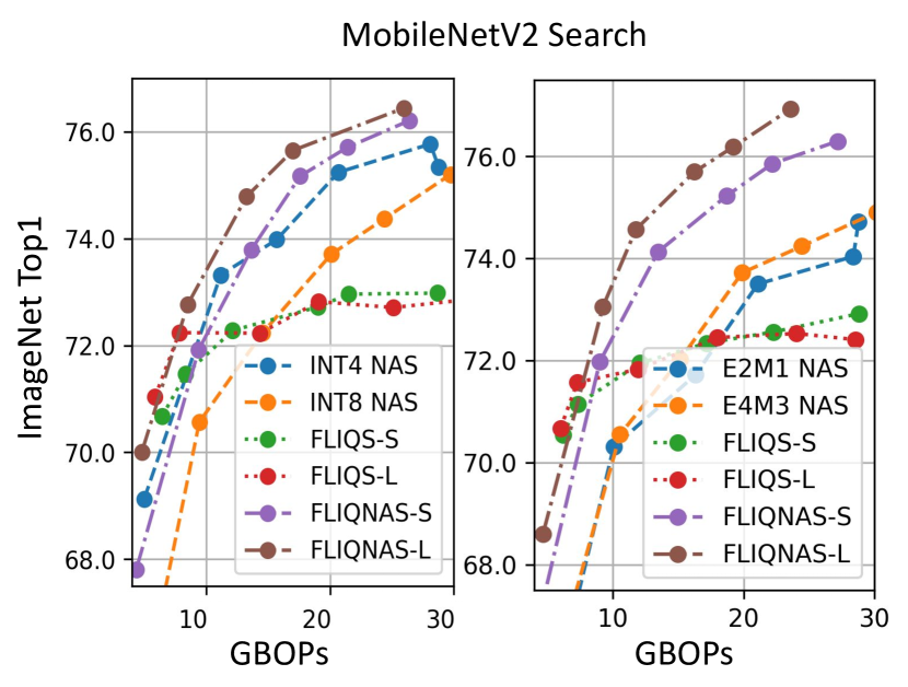
Figure 6: MobileNetV2 FLIQNAS – FLIQNAS outperforms APQ in a similar quantization and neural architecture search space. APQ additionally includes tunable depth within the inverted bottleneck blocks, and APQ-{A,B,C} represent different targets and mild variations in method. In addition, the combination of quantization search and neural architecture search outperforms the two methods separately on integer and floating-point formats.

MobileNetV2: The MobileNetV2 FLIQNAS search expands the previous format search spaces by incorporating tunable filter widths on inverted bottleneck projection layers and adjustable kernel sizes on central depthwise layers. Altogether, there are 230 tunable values leading to a search space of over $10^{100}$ configurations for FLIQNAS-S. This search space is significantly larger than that of the original MobileNetV2 FLIQS-S with 53 options and approximately $10^{25}$ configurations.

Figure 6 compares FLIQNAS to FLIQS and quantized NAS, which fixes the quantization format for all layers and only searches for the architecture. It shows that FLIQS-S and FLIQS-L searches perform well for low model costs, yet as the model scales to higher costs, the compute is better allocated by increasing the size of the architectural components. In this region, both quantized NAS and FLIQNAS yield the best performance. For all model costs, FLIQNAS-L is able to reach the Pareto-optimal tradeoff of accuracy and model cost. Lastly, when compared at identical cost targets, floating-point FLIQNAS surpasses the performance of the integer search space.

In Figure 6, we include a FLIQNAS comparison against APQ Wang et al. (2020), which performs a joint architecture, pruning, and quantization search by using a large once-for-all network. Its search space is similar and includes multiple kernel sizes, channel widths, and integer bitwidths built on top of the original MobileNetV2 architecture. This table shows that for similar GBOPs, FLIQNAS leads to higher accuracy over APQ across its three published design points. Further layer-wise analysis of these results is located in Appendix A.7.

Recommendation Model: In Appendix A.13, we further evaluate FLIQNAS with an multi-layer perceptron recommendation model on the Criteo dataset, which is the most popular public advertisement click-through-rate (CTR) prediction benchmark. This section similarly indicates that FLIQNAS-L performs better than FLIQS-L especially at larger model costs, and both techniques show better quality and performance trade-offs than uniform quantization alone.

7 Conclusion

As AI hardware supports an increasing number of numerical formats, DNN quantization search to integer and low-precision floating-point grows increasingly important for reducing memory and compute. This paper proposes FLIQS, the first one-shot RL-based integer and low-precision floating-point quantization search without retraining. Compared to prior work, FLIQS can achieve higher accuracy without involving additional fine-tuning or retraining steps by introducing a cosine entropy regularization schedule. Moreover, as an RL-based method, it reduces the amount of memory needed for weights, activations, and gradients during the search compared to recent differentiable NAS searches.

These enhancements accelerate research progress and enable quantization searches on larger search spaces and more substantial models, such as DeiT-B16, which has 10 times the model cost as BF16 MobileNetV2. In addition, FLIQS conducts the first floating-point quantization search and produces mixed-precision models that outperform the latest works on FP8 formats. When further combined with architecture search, it identifies even stronger MobileNetV2 models than NAS and quantization search alone. It further suggests that for a fixed compute budget, larger models benefit from increasing architectural dimensions over bitwidth. Overall, FLIQS represents an efficient framework for searching multi-precision models on current hardware and gives further insight into model and hardware co-design for future accelerator generations.

Appendix A Appendix

The following sections contain additional experimental details, small experiments, ablation studies, and example output bitwidths. The listed hyper-parameters attempt to make the results more reproducible and interpretable. In addition, the small-scale experiments motivate certain hyper-parameter selections discussed in the main paper. And finally, the example configurations give more insight into how FLIQS allocates bitwidth across different models and cost targets.

A.1 Example Configurations

FLIQS bitwidth configurations vary based on the model and search space. Figure 7 shows a set of configurations for FLIQS-L and FLIQS-S searches on a ResNet18 across four different model cost targets. Lower bitwidths are represented with colors closer to red and higher bitwidths are closer to green. This figure shows that FLIQS typically gives higher bitwidth to the first and last layers of the model. It also consistently gives higher bitwidths to the 1x1 convolution on the upper branch, and although not obvious in this figure, it usually allocates more bitwidth to the earlier stages of the model compared to later stages.

Figure 8 shows example bitwidth configurations for all models evaluated. It reveals that ResNet50 has similar trends to ResNet18: more bitwidth for the first and last layers, 1x1 convolutions on the upper branch, and generally more in the early stages. Unlike the ResNet models, MobileNetV2 has a main block that comprises a sequence of a pointwise convolution, depthwise convolution, and then pointwise convolution. FLIQS allocates more bitwidth to the central 3x3 depthwise convolution in this block (groups of three in the figure). InceptionV3 has a more complicated branched architecture of 1x1, 3x3, and 5x5 convolutions. This block is shown in the figure as the repeated structure of one, three, two, and then one convolution, from top to bottom. FLIQS likewise gives more bitwidth to the earlier stages of InceptionV3 and its first and last layers. Additionally, it increases the precision of the 1x1 convolutions on the top and bottom of the repeated block.

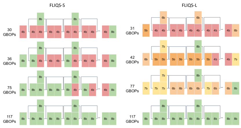
Figure 7: ResNet18 Integer FLIQS – Output configurations depend on the model, model cost target, and supported bitwidths. FLIQS-S uses 4 and 8 bits as the search space, while FLIQS-L uses 4 to 8 bits, inclusive. For both variants, FLIQS generally allocates higher bits to the first and last layers, with a slight preference for the last layer. It also assigns more bits to the small upper 1x1 convolutions and more bits to the first 3x3 convolution within a block.

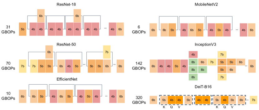
Figure 8: Integer FLIQS-L Examples

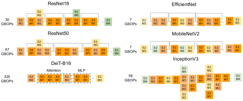
Figure 9: Floating-Point FLIQS-L Examples

Figure 10: Start Step

Start Step	Top-1
1000	75.59
2000	75.59
4000	76.11
6000	76.05
8000	76.02
10000	76.03
15000	75.94
20000	75.93
25000	75.54
30000	74.19

Figure 11: STD Multiple

STD Multiple	Top-1
1	63.39
2	67.79
3	68.02
4	67.91
5	67.19
6	67.00
7	66.15
8	64.91

Figure 12: Profile Batches

Profile Batches	Top-1
1	67.92
5	68.09
10	68.00
50	67.75
100	68.02

A.2 Two-Phase Quantization

These shared weights are quantized dynamically with a method adapted from the open-source library Accurate Quantized Training (AQT) Abdolrashidi et al. [2021], which supports both integer and emulated low-precision floating point quantization. This process can be summarized as:

$$x_{q}=\lfloor s\cdot\sigma(x_{f};\sigma_{t})\rceil$$ (15)

$$\sigma(x_{f};\sigma_{t})=\max(-\sigma_{t},\min(x_{f},\sigma_{t}))$$ (16)

where $x_{q}$ is the quantized value, $x_{f}$ is the original full-precision number, $s$ is the scale factor, and $\sigma_{t}$ denotes the clipping threshold. In addition, $\sigma(\cdot)$ represents a clipping function, and $\lfloor\cdot\rceil$ represents a generic rounding function that pushes the value to the nearest integer or low-precision floating-point value.

The scale factor $s$ normalizes the input to the chosen maximum representable number and then rescales to the maximum quantized value. The clipping threshold and scale factor are determined by the run-time statistics of the weights and activations. Additionally, FLIQS uses a two-phase quantization approach where the weights and activations begin quantization at different training steps, as shown in Figure 2.

The two-phase quantization approach has been found empirically to improve the final accuracy of the model. In the first phase, only the weights are quantized and in the second phase, the weights and activations are quantized. The start step of the second phase has a large effect on the final accuracy. Table 12 shows the effect of sweeping the starting step for activation quantization on a ResNet50 trained to 30,200 steps. On one extreme, with the second phase starting as soon as possible, this method degenerates into a single-phase quantization method where weight and activation quantization begin immediately. On the other extreme, where the second phase begins as late as possible, it becomes a hybrid QAT-PTQ method where the weights are quantized during training and the activations are quantized after training.

Table 12 shows that accuracy peaks around 15-20% of the total training time. For this reason, FLIQS uses 7500 steps as the start step for activation quantization for ResNets and InceptionV3, which train to 30,200 steps, and 20,000 as the start step for MobileNetV2, EfficientNet, and DeiT, which train to 112,000 steps or longer.

The quantization method additionally depends on the activation clipping threshold, which is calculated as a multiple of the profiled activation standard deviations per layer. With too small a clipping threshold, there is lower rounding error on the more numerous central values distribution, yet there is significant clipping error on the larger values. With too large a threshold, there is more rounding error on the central values and less clipping error on the larger values.

This trade-off is demonstrated empirically in Table 12, where standard deviation multiples are swept from 1 to 8 and applied globally to a ResNet18. This table shows that the best accuracy are achieved around 3-4 times the standard deviation in ResNet18. For simplicity, we apply this multiple to all models for our experiments. Table 12 shows that the final accuracy is not sensitive to the number of profiling batches. This is likely because we use a large batch size of 2048, and since it is shuffled, it likely already provides a strong estimate of the statistics.

A.3 Training Hyper-Parameters

The training hyper-parameters are chosen to be close to original paper hyper-parameters or recent related work. Table 4 shows the hyper-parameters used to produce Table 1 and Figure 5.

Table 4: Training Hyper-Parameters – Training Hyper-parameters for all quantization search table results. Same hyper-parameters are used to produce the Pareto-curve figures, although the total training time is reduced along with dependent hyper-parameters, e.g. activation quantization start step.

Parameter	ResNets	DeiT-B16	MBV2
	IncV3		EffNet
LR Schedule	Cos	Cos	Exp
LR Base	2.64	4e-3	0.256
LR Warmup	10	30	15
Optimizer	SGD	AdamW	RMSProp
Epochs	350	400	360
Act. Quant Start	15,000	15,000	18,000
ST Multiple	4	4	4%

A.4 Search Hyper-Parameters

For our search, the RL controller warmup period lasts the first 25% of the training It uses an Adam optimizer with learning rate of 4.6E-3 and momentum of .95. The loss function is a standard softmax cross entropy loss with a label smoothing coefficient set to 0.1. A cosine entropy regularization schedule is applied to all runs beginning with no regularization and ending with $\beta_{H}=.5$. For QNAS, during the RL controller warmup period, the branches corresponding to various kernel sizes are sampled jointly with a probability schedule. This schedule begins at 1 at the beginning of training and decreases linearly to 0 at the end of the warmup period. After the warmup period, only a single branch is sampled at a time.

A.5 Search Space

Table 5: Search Space: FLIQS-S is a small search space designed to target existing hardware support, while FLIQS-L is a large search space useful for co-design with custom hardware. The floating-point FLIQS-L space demonstrates the scalability of RL-based approaches

	FLIQS-S	FLIQS-L
Integer	INT4, INT8, BF16	INT4, INT5, INT6,
		INT7, INT8, BF16
Floating	E2M1, E4M3, BF16	E2M1, E2M2, E2M3, E2M4,
Point		E2M5, E3M1, E3M2, E3M3,
		E3M4, E4M1, E4M2, E4M3,
		E5M1, E5M2, E6M1, BF16

In general, the search spaces used with FLIQS should reflect the capabilities of the target hardware. Small search spaces are useful for adapting a model to existing hardware such as the TPUv3 or NVIDIA A100. Large search spaces are useful for reconfigurable hardware such as the AMD Xilinx UltraScale+ FPGA and for co-designing models with future accelerators. The largest search space evaluated in this work includes 16 floating-point formats.

For the integer FLIQS-S search space, we include INT4, INT8, and BF16. These are the standard formats supported in modern GPU micro-architectures, such as NVIDIA Ampere. Many platforms additionally support FP16, yet this format typically performs worse than BF16 in most common use cases, so it omitted. For integer FLIQS-L, we fill in the values between INT4 and INT8 primarily considering custom hardware with integer support. For example, bit-serial deep learning engines can take advantage of this additional flexibility.

For floating-point FLIQS-S, we include three formats to be consistent with the integer search variant. BF16 is the most common half-precision format, E4M3 is the FP8 variant most useful for inference (E4M2 primarily used for gradients), and E2M1 is a custom FP4 format. For FLIQS-L, we include all the formats with total bitwidths between four and eight.

All custom formats support subnormals and do not support infinity. The bias terms are selected so the exponent range is symmetric about zero. However, this bias term is not relevant to FLIQS, since continuing from prior work Abdolrashidi et al. [2021], Micikevicius et al. [2022], it uses a profiled scale factor during training and search. This means that the bias term combines with the profiled scale factor and has no additional effect. Therefore, the dynamic range is controlled more by the additional scale factor than the format itself and can adequately scale to various data distributions; the format instead primarily determines the distribution of quantization points (non-linear for floating-point and linear for integer ).

A.6 Search Performance

	Memory (MiB)			Search
	Gradient	Weight	Activation	Parameters
FLIQS	46.8	23.4	73.6	51
Branched	92.6	70.2	220.8	51

Table 6: ResNet18 Memory – the estimated memory breakdown for a ResNet18 model during quantization search on the FLIQS-S search space. Branched represents the class of quantization searches that create multiple branches during their search. Batch size is fixed at 32, model weights and activations are stored in half-precision, and gradients are full-precision with no gradient checkpointing. Search Parameters represents the additional parameters necessary for the search process. FLIQS and branched methods require an additional parameter for each searched layer for each searched option.

A.7 QNAS Analysis

In general, QNAS searches tend to allocate more of their compute to architectural components, especially at high cost targets. This behavior is shown in Figure 6, where expanding quantization searches to include flexible channels and kernel size dimensions increases the accuracy of the model at similar costs. Within these architectural components, typically the channel dimension is increased before the kernel size to reach cost targets. This could be due to the fundamental difference between kernel size and channel width; kernel size reflects the ability to aggregate information faster across spatial dimensions and channel width controls the depth of a neural network representation.

The channel dimension allocations also show an interesting trend in that lower bitwidths typically receive a larger number of channels. This is intuitive since increasing the channel width can potentially recuperate losses in representational ability from the lower bitwidth. There is a weaker trend in this direction with kernel size, where the kernel size can tend to be larger with lower bitwidths, although it is not as strong.

A.8 Analysis Setup

For shifting error and clipping analysis, we simulate the data distributions commonly found within neural networks. For this, we use Gaussian and Laplacian distributions and inject additional outlier values. These outliers are set at $3\times$ the maximum value in the original tensor and are injected at various rates from 1:10 to 1:10000. These outliers are especially common in activation tensors.

For the shifting error, we then sample 1000 tensors independently at random, and quantize them with two different symmetric linear quantizers that vary only in their bitwidths. We then calculate the RMS error between the two output tensors and average over all 1000 tensors. Finally, we fit the best exponential function with the form: $Ae^{(-Bx)}+C$.

Similarly, for the clipping analysis, we sample 100 tensors and calculate the quantization error between the original FP32 and quantized tensors for each percentile value. For the percentiles, we use a linear grid of 100 values from [1, 101]. We then plot the average MSE error over the 100 tensors and separately plot the optimal percentile. We experimented with different metrics, such as the Kullback-Liebler (KL) divergence, yet these did not lead to qualitatively different results.

A.9 Mantissa Sweep

Table 7: FP8 Sweep – Sweep over possible FP8 values and evaluate Top-1 accuracy on ImageNet. All methods use an exponent bias of 11.

Mode	ResNet18	ResNet50	MobileNetV2	InceptionV3
E1M6	71.72	77.80	73.20	76.53
E2M5	71.70	77.74	73.14	76.36
E3M4	71.69	77.55	73.17	76.48
E4M3	71.69	77.66	72.65	76.30
E5M2	71.59	76.90	72.07	76.15

Table 7 shows the general effects of different possible FP8 formats on ImageNet accuracy. The models are generally resilient to FP8 quantization with MobileNetV2 having the largest accuracy degradation with the E5M2 format. This is analogous to integer quantization, where typically INT8 is sufficient for most models to maintain neutral accuracy and where MobileNetV2 is more sensitive to low-bit quantization. In this table, the accuracy trends upward with more mantissa bits, and therefore not only do they determine the majority of the area in floating-point units, they increase the accuracy of the models. This leads to the classical accuracy-performance trade-off that floating-point quantization search attempts to navigate for optimal configurations. Yet for hardened accelerators, the peak throughput for different FP8 formats is the same, and therefore higher mantissa bitwidth is preferable.

A.10 Cost Model FPGA Validation

Table 3 shows the hardware area estimates and accuracy of a set of ResNet-18 models on an AMD Xilinx UltraScale+ FPGA, implemented using Vivado HLS Xilinx [2020]. Since the whole model does not fit on the board, we estimate the cost with the first residual block in the model, which consists of two convolutional layers on one branch, and a pointwise convolution on the other, followed by their sum. Since all MAC operations are mapped to look-up tables (LUTs), the LUT count acts as a proxy for the area and power overhead of the model. The precision settings for FLIQS-L are taken from actual runs and represent the general bitwidth allocation to the ResNet blocks, although there may be some deviation within individual blocks.

This table shows that LUTs scale quadratically with the precision bitwidth. Since the LUTs act as a proxy for area, this verifies the core assumption of the BOPs model (Section 1) that BOPs are proportional to the model area and power on chip. This table also confirms the overhead from these searched models is indeed relatively small compared to the accuracy improvements shown in Table 1.

A.11 Retraining vs. No Retraining

With sufficient entropy regularization, retraining the model after FLIQS is unnecessary. Table 8 shows a sweep for ResNet18 with and without retraining. With retraining, the search occurs as described in Section 3, except that the best configuration is taken and retrained from scratch for the original training length. The table shows natural variance between the retraining and no-retraining methods, but there is no noticeable advantage to retraining across model widths.

Table 8: Retraining ResNet-18

ImageNet Top1
Format	$\mathbf{0.5\times}$	$\mathbf{0.75\times}$	$\mathbf{1.0\times}$	$\mathbf{1.25\times}$	$\mathbf{1.5\times}$	$\mathbf{2.0\times}$
FLIQS-S	59.08	64.93	69.92	71.94	73.32	75.06
+ Retrain	59.00	66.47	69.53	71.63	73.20	74.95
FLIQS-L	60.11	66.28	69.56	71.61	73.12	74.83
+ Retrain	60.10	66.39	69.56	71.58	73.02	74.78

A.12 All Models

Figure 14 and Figure 14 plot all models with corresponding colors for methods and corresponding symbols for models. It shows that FLIQS MobileNetV2 and EfficientNet models consistently outperform other models in terms of accuracy and model cost, and BF16 models consistently perform the worst. This is expected since, as their name suggests, these models are designed specifically to be efficient and both use inverted bottleneck structures to reduce overall compute. The worst performing model overall is ResNet18, which is followed in the higher model costs by ResNet50.

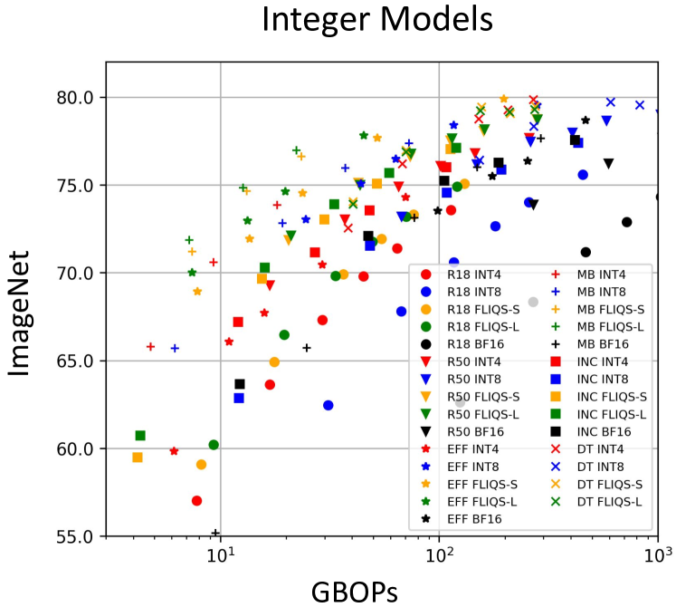
Figure 13: Integer All Models – All models plotted including the uniform precision baselines and searched FLIQS models.

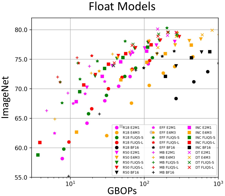
Figure 14: Floating-Point All Models – All models plotted including the uniform precision baselines and FLIQS models.

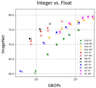
Figure 15: Floating-Point vs. Integer FLIQS-L – Floating-point models typically outperform their integer counter-parts.

A.13 Recommendation Model

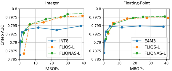
Figure 16: Recommender FLIQNAS – Models are trained on the Criteo dataset and evaluated by AUC (Area Under the ROC Curve) vs. millions of BOPs (MBOPs). Both FLIQNAS and FLIQS perform better than the INT8 and E4M3 baselines.

Next, we briefly explore FLIQNAS on recommendation models using the Criteo dataset CriteoLabs [2014], which is the most popular public advertisement click-through-rate (CTR) prediction benchmark. We evaluate a multi-layer perceptron (MLP) model with four hidden layers and layer factorization technique Golub and Van Loan [2013] similar to the method used in DCN-V2 (Deep & Cross Network) Wang et al. [2021]. We use the AUC metric for evaluation, and list additional details about the dataset, model architecture and search space.

Figure 16 compares FLIQNAS and FLIQS with uniformly quantized models on both integer and float quantization. We focus only on FLIQS-L due to the small search space and do not include the uniformly quantized INT4 and E2M1 models since they show significant quality loss. Figure 16 shows that FLIQNAS-L performs better than FLIQS-L especially at larger MBOPs. Both of them show better quality and performance trade-offs than uniform quantization.

Criteo: The Criteo dataset CriteoLabs [2014] contains user logs over a period of 7 days with a total of 45M examples. Each example has 13 continuous features and 26 categorical features with a binary label indicating if an advertisement was clicked or not.

Architecture: The recommendation model architecture starts with an embedding layer to project the sparse categorical features into dense vectors. The embedded vectors are then concatenated with the continuous features and fed into the MLP with four hidden layers and low-rank on each layer to reduce the computational cost.

Search Space: For FLIQS-L, the search space uses the same configurations for integer or floating-point search on each layer. For FLIQNAS-L, besides the quantization search space, we also include $128$ and $512\times[0.25,0.5,0.75,1.0,1.25,1.5,1.75,2.0]$ for rank values and layer widths respectively on each layer.

A.14 Additional Pareto Tables

This section lists all of the raw data used to produce the Pareto curves in Figure 5.

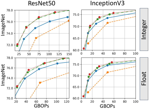
Figure 17: Additional Pareto Curves – Additional integer and floating-point Pareto curves that could not fit in the main paper.

ImageNet Top1
Format	$\mathbf{0.5\times}$	$\mathbf{0.75\times}$	$\mathbf{1.0\times}$	$\mathbf{1.25\times}$	$\mathbf{1.5\times}$	$\mathbf{2.0\times}$
BF16	62.63	68.34	71.17	72.89	74.31	75.56
INT4	57.03	63.64	67.32	69.79	71.39	73.57
INT8	62.46	67.80	70.60	72.65	74.01	75.58
FLIQS-S	59.08	64.93	69.92	71.94	73.32	75.06
FLIQS-L	60.11	66.28	69.56	71.61	73.12	74.83
+ ($\beta_{H}^{\cos}$)	60.21	66.47	69.83	71.76	73.19	74.91

GBOPs
Format	$\mathbf{0.5\times}$	$\mathbf{0.75\times}$	$\mathbf{1.0\times}$	$\mathbf{1.25\times}$	$\mathbf{1.5\times}$	$\mathbf{2.0\times}$
BF16	124.5	268.8	467.7	721.3	1030	1810
INT4	7.78	16.80	29.23	45.08	64.35	113.1
INT8	31.13	67.19	116.9	180.3	257.4	452.5
FLIQS-S	8.18	17.68	36.46	54.60	76.35	130.7
FLIQS-L	9.04	19.09	32.33	49.22	69.20	120.2
+ ($\beta_{H}^{\cos}$)	9.30	19.58	33.54	49.57	70.54	120.8

Figure 18: Integer ResNet-18

ImageNet Top1
Format	$\mathbf{0.5\times}$	$\mathbf{0.75\times}$	$\mathbf{1.0\times}$	$\mathbf{1.25\times}$	$\mathbf{1.5\times}$	$\mathbf{2.0\times}$
INT4	69.27	73.03	74.91	76.07	76.81	77.68
INT8	73.20	76.17	77.47	77.98	78.66	79.00
FLIQS-S	71.85	75.11	76.62	77.52	78.06	78.76
FLIQS-L	71.56	74.67	76.52	77.37	78.02	78.73
+ ($\beta_{H}^{\cos}$)	72.12	75.01	76.79	77.66	78.17	78.72
BF16	73.87	76.22	77.68	78.45	78.82	79.14

GBOPs
Format	$\mathbf{0.5\times}$	$\mathbf{0.75\times}$	$\mathbf{1.0\times}$	$\mathbf{1.25\times}$	$\mathbf{1.5\times}$	$\mathbf{2.0\times}$
INT4	16.84	37.16	65.43	101.6	145.8	257.9
INT8	67.35	148.7	261.7	406.5	583.1	1031
FLIQS-S	20.49	42.87	73.66	112.7	160	279.3
FLIQS-L	20.51	41.13	71.57	112.9	156.4	273.5
+ ($\beta_{H}^{\cos}$)	21.03	43.55	74.49	114.8	161.5	282
BF16	269.4	594.6	1047	1626	2332	4126

Figure 19: Integer ResNet-50

ImageNet Top1
Format	$\mathbf{0.25\times}$	$\mathbf{0.5\times}$	$\mathbf{1.0\times}$	$\mathbf{1.4\times}$	$\mathbf{2.0\times}$
BF16	55.18	65.72	73.13	76.00	77.64
INT4	40.62	54.11	65.80	70.60	73.85
INT8	55.09	65.70	72.83	75.95	77.37
FLIQS-S	50.78	63.03	71.21	74.64	76.61
FLIQS-L	52.38	63.15	71.73	74.99	77.01
+ ($\beta_{H}^{\cos}$)	52.11	63.35	71.87	74.83	76.98

GBOPs
Format	$\mathbf{0.25\times}$	$\mathbf{0.5\times}$	$\mathbf{1.0\times}$	$\mathbf{1.4\times}$	$\mathbf{2.0\times}$
BF16	9.52	24.87	77.00	149.0	291.2
INT4	0.595	1.55	4.81	9.31	18.20
INT8	2.38	6.21	19.25	37.20	72.80
FLIQS-S	1.16	2.90	7.42	13.21	23.51
FLIQS-L	1.06	2.38	7.06	12.70	22.26
+ ($\beta_{H}^{\cos}$)	1.02	2.42	7.21	12.69	22.31

Figure 20: Integer MobileNetV2

ImageNet Top1
Format	$\mathbf{0.25\times}$	$\mathbf{0.5\times}$	$\mathbf{0.75\times}$	$\mathbf{1.0\times}$	$\mathbf{1.5\times}$
BF16	63.65	72.10	75.24	76.26	77.55
INT4	53.20	67.20	71.16	73.55	76.00
INT8	62.86	71.52	74.56	75.87	77.38
FLIQS-S	59.49	69.66	73.04	75.07	77.05
+ ($\beta_{H}^{\cos}$)	60.72	70.28	73.91	75.67	77.12

GBOPs
Format	$\mathbf{0.25\times}$	$\mathbf{0.5\times}$	$\mathbf{0.75\times}$	$\mathbf{1.0\times}$	$\mathbf{1.5\times}$
BF16	48.69	193.1	433.3	769.2	1728
INT4	3.04	12.07	27.08	48.08	108.0
INT8	12.17	48.28	108.3	192.3	432.0
FLIQS-S	4.18	15.53	29.88	52.02	112.5
+ ($\beta_{H}^{\cos}$)	4.31	15.99	33.17	59.16	119.9

Figure 21: Integer InceptionV3

ImageNet Top1
Format	B0	B1	B2	B3	B4
BF16	73.53	75.50	76.36	78.68	80.35
INT4	59.83	66.08	67.71	70.46	74.29
INT8	73.04	75.08	76.48	78.39	79.55
FLIQS-S	68.94	71.92	74.53	77.67	79.89
FLIQS-L	70.51	73.23	75.41	77.96	80.03
+ ($\beta_{H}^{\cos}$)	70.01	72.96	74.62	77.81	79.92

GBOPs
Format	B0	B1	B2	B3	B4
BF16	98.61	175.5	254.0	467.3	1124
INT4	6.16	10.97	15.88	29.21	70.25
INT8	24.65	43.89	63.50	116.8	281.0
FLIQS-S	7.86	13.62	23.81	52.30	198.0
FLIQS-L	7.40	13.21	21.62	49.38	187.0
+ ($\beta_{H}^{\cos}$)	7.42	13.32	19.85	45.26	187.1

Figure 22: Integer EfficientNet

ImageNet Top1
Format	$\mathbf{0.25\times}$	$\mathbf{0.375\times}$	$\mathbf{0.5\times}$	$\mathbf{0.75\times}$	$\mathbf{0.875\times}$	$\mathbf{1.0\times}$
INT4	66.51	72.53	76.19	78.75	79.26	79.84
INT8	70.77	76.41	78.33	79.71	79.55	79.49
FLIQS-S	66.36	74.05	76.96	79.44	79.05	79.47
FLIQS-L	67.04	73.93	77.10	79.27	79.27	79.35
+ ($\beta_{H}^{\cos}$)	67.78	73.90	76.88	79.23	79.16	79.28

GBOPs
Format	$\mathbf{0.25\times}$	$\mathbf{0.375\times}$	$\mathbf{0.5\times}$	$\mathbf{0.75\times}$	$\mathbf{0.875\times}$	$\mathbf{1.0\times}$
INT4	20.29	38.42	67.96	152.1	206.8	269.8
INT8	80.94	153.5	271.5	608.1	826.6	1079
FLIQS-S	20.31	40.52	70.74	156.3	211.7	275.4
FLIQS-L	21.08	39.55	69.12	153.9	208.8	272.0
+ ($\beta_{H}^{\cos}$)	21.47	40.45	70.57	154.5	210.4	273.2

Figure 23: Integer DeiT-B16

ImageNet Top1
Format	$\mathbf{0.5\times}$	$\mathbf{0.75\times}$	$\mathbf{1.0\times}$	$\mathbf{1.25\times}$	$\mathbf{1.5\times}$	$\mathbf{2.0\times}$
BF16	62.63	68.34	71.17	72.89	74.31	75.56
E2M1	58.17	64.18	67.96	70.43	72.08	74.22
E4M3	62.06	67.57	70.56	72.66	73.75	75.43
FLIQS-S	59.80	65.77	68.89	72.10	73.50	75.26
+ ($\beta_{H}^{\cos}$)	60.99	66.61	70.01	71.92	73.32	74.80

GBOPs
Format	$\mathbf{0.5\times}$	$\mathbf{0.75\times}$	$\mathbf{1.0\times}$	$\mathbf{1.25\times}$	$\mathbf{1.5\times}$	$\mathbf{2.0\times}$
BF16	124.5	268.8	467.7	721.3	1030	1810
E2M1	7.78	16.80	29.23	45.08	64.35	113.1
E4M3	31.13	67.19	116.9	180.3	257.4	452.5
FLIQS-S	8.18	17.68	30.80	54.60	76.35	128.2
+ ($\beta_{H}^{\cos}$)	9.60	19.48	32.78	50.01	68.43	118.2

Figure 24: Floating-Point ResNet-18

ImageNet Top1
Format	$\mathbf{0.5\times}$	$\mathbf{0.75\times}$	$\mathbf{1.0\times}$	$\mathbf{1.25\times}$	$\mathbf{1.5\times}$	$\mathbf{2.0\times}$
BF16	73.87	76.22	77.68	78.45	78.82	79.14
E2M1	70.24	73.91	75.77	76.89	77.40	78.01
E4M3	73.09	75.86	77.42	78.13	78.42	78.97
FLIQS-S	72.16	75.14	76.84	77.83	78.22	78.94
+ ($\beta_{H}^{\cos}$)	72.39	75.61	76.95	78.00	78.24	78.81

GBOPs
Format	$\mathbf{0.5\times}$	$\mathbf{0.75\times}$	$\mathbf{1.0\times}$	$\mathbf{1.25\times}$	$\mathbf{1.5\times}$	$\mathbf{2.0\times}$
BF16	269.4	594.6	1047	1626	2332	4126
E2M1	16.84	37.16	65.43	101.6	145.8	257.9
E4M3	67.35	148.7	261.7	406.5	583.1	1031
FLIQS-S	21.72	42.87	74.28	112.7	160.0	279.2
+ ($\beta_{H}^{\cos}$)	21.93	44.70	76.43	115.6	165.6	297.9

Figure 25: Floating-Point ResNet-50

ImageNet Top1
Format	$\mathbf{0.25\times}$	$\mathbf{0.5\times}$	$\mathbf{1.0\times}$	$\mathbf{1.4\times}$
BF16	55.18	65.72	73.13	76.00
E2M1	—	52.32	66.29	69.26
E4M3	53.98	64.85	72.63	75.86
FLIQS-S	50.76	62.58	71.14	74.34
+ ($\beta_{H}^{\cos}$)	51.11	63.65	71.97	75.26

GBOPs
Format	$\mathbf{0.25\times}$	$\mathbf{0.5\times}$	$\mathbf{1.0\times}$	$\mathbf{1.4\times}$
BF16	9.52	24.87	77.00	149.0
E2M1	0.595	1.55	4.81	9.31
E4M3	2.38	6.21	19.25	37.20
FLIQS-S	1.22	2.69	7.35	12.6
+ ($\beta_{H}^{\cos}$)	0.95	2.36	6.77	12.37

Figure 26: Floating-Point MobileNetV2

ImageNet Top1
Format	$\mathbf{0.25\times}$	$\mathbf{0.5\times}$	$\mathbf{0.75\times}$	$\mathbf{1.0\times}$	$\mathbf{1.5\times}$
BF16	63.65	72.10	75.24	76.26	77.55
E2M1	54.14	67.80	72.09	74.55	76.35
E4M3	62.65	71.50	74.49	75.94	77.39
FLIQS-S	58.78	69.50	73.43	75.28	77.03
+ ($\beta_{H}^{\cos}$)	60.90	70.63	74.16	75.94	77.43

GBOPs
Format	$\mathbf{0.25\times}$	$\mathbf{0.5\times}$	$\mathbf{0.75\times}$	$\mathbf{1.0\times}$	$\mathbf{1.5\times}$
BF16	48.69	193.1	433.3	769.2	1728
E2M1	3.04	12.07	27.08	48.08	108.0
E4M3	12.17	48.28	108.3	192.3	432.0
FLIQS-S	3.66	13.46	29.16	51.65	111.4
+ ($\beta_{H}^{\cos}$)	3.89	15.23	32.86	56.15	124.2

Figure 27: Floating-Point InceptionV3

ImageNet Top1
Format	B0	B1	B2	B3	B4
BF16	73.53	75.50	76.36	—	—
E2M1	62.45	67.49	69.14	71.22	76.12
E4M3	72.99	75.36	76.20	78.17	79.52
FLIQS-S	67.60	71.63	74.67	78.05	80.30
+ ($\beta_{H}^{\cos}$)	71.13	74.34	75.58	78.03	80.29

GBOPs
Format	B0	B1	B2	B3	B4
BF16	98.61	175.5	254.0	—	—
E2M1	6.16	10.97	15.88	29.21	70.25
E4M3	24.65	43.89	63.50	116.8	281.0
FLIQS-S	7.77	13.58	23.26	55.15	203.3
+ ($\beta_{H}^{\cos}$)	7.30	13.00	19.61	36.6	212.9

Figure 28: Floating-Point EfficientNet

ImageNet Top1
Format	$\mathbf{0.25\times}$	$\mathbf{0.375\times}$	$\mathbf{0.5\times}$	$\mathbf{0.75\times}$	$\mathbf{0.875\times}$	$\mathbf{1.0\times}$
E2M1	66.63	73.88	76.35	80.10	79.04	79.49
E4M3	71.19	76.96	78.85	79.13	79.90	79.17
FLIQS-S	67.27	73.95	77.52	79.24	79.56	79.27
FLIQS-L	68.25	74.36	77.35	78.89	79.56	79.54

GBOP
Format	$\mathbf{0.25\times}$	$\mathbf{0.375\times}$	$\mathbf{0.5\times}$	$\mathbf{0.75\times}$	$\mathbf{0.875\times}$	$\mathbf{1.0\times}$
E2M1	20.29	38.42	67.96	152.1	206.8	269.8
E4M3	80.94	153.5	271.5	608.1	826.6	1079
FLIQS-S	20.3	38.42	70.74	156.3	211.7	275.4
FLIQS-L	21.08	39.40	68.49	152.9	207.7	270.8

Figure 29: Floating-Point DeiT-B16

References

- Abdelfattah et al. (2018) Mohamed Saleh Abdelfattah, David Han, Andrew Bitar, Roberto Dicecco, Shane O’Connell, Nitika Shanker, Joseph Chu, Ian Prins, Joshua Fender, Andrew C. Ling, and Gordon R. Chiu. DLA: Compiler and FPGA Overlay for Neural Network Inference Acceleration. 28th International Conference on Field Programmable Logic and Applications (FPL), pages 411–4117, 2018.
- Abdolrashidi et al. (2021) AmirAli Abdolrashidi, Lisa Wang, Shivani Agrawal, Jonathan Malmaud, Oleg Rybakov, Chas Leichner, and Lukasz Lew. Pareto-optimal quantized resnet is mostly 4-bit. Conf. on Computer Vision and Pattern Recognition (CVPR), 2021.
- Bai et al. (2021) Haoping Bai, Meng Cao, Ping Huang, and Jiulong Shan. BatchQuant: Quantized-for-all Architecture Search with Robust Quantizer. Advances in Neural Information Processing Systems (NeurIPS), 2021.
- Bender et al. (2020) Gabriel Bender, Hanxiao Liu, Bo Chen, Grace Chu, Shuyang Cheng, Pieter-Jan Kindermans, and Quoc Le. Can weight sharing outperform random architecture search? an investigation with tunas. Conf. on Computer Vision and Pattern Recognition (CVPR), 2020.
- Cai et al. (2020) Yaohui Cai, Zhewei Yao, Zhen Dong, Amir Gholami, Michael W. Mahoney, and Kurt Keutzer. ZeroQ: A Novel Zero Shot Quantization Framework. Conf. on Computer Vision and Pattern Recognition (CVPR), 2020.
- Cai and Vasconcelos (2020) Zhaowei Cai and Nuno Vasconcelos. Rethinking Differentiable Search for Mixed-Precision Neural Networks. Conf. on Computer Vision and Pattern Recognition (CVPR), 2020.
- Chen et al. (2018) Tianqi Chen, Thierry Moreau, Ziheng Jiang, Lianmin Zheng, Eddie Yan, Haichen Shen, Meghan Cowan, Leyuan Wang, Yuwei Hu, Luis Ceze, Carlos Guestrin, and Arvind Krishnamurthy. TVM: An automated End-to-End optimizing compiler for deep learning. In 13th USENIX Symposium on Operating Systems Design and Implementation (OSDI 18), pages 578–594, Carlsbad, CA, Oct 2018. USENIX Association. ISBN 978-1-939133-08-3. URL https://www.usenix.org/conference/osdi18/presentation/chen.
- Choi et al. (2018) Jungwook Choi, Zhuo Wang, Swagath Venkataramani, Pierce I-Jen Chuang, Vijayalakshmi Srinivasan, and Kailash Gopalakrishnan. Pact: Parameterized clipping activation for quantized neural networks. arvix, 2018.
- CriteoLabs (2014) CriteoLabs. Kaggle Display Advertising Challenge Dataset. http://labs.criteo.com/2014/02/kaggle-display-advertising-challenge-dataset, 2014.
- Dong et al. (2019) Zhen Dong, Zhewei Yao, Amir Gholami, Michael W. Mahoney, and Kurt Keutzer. HAWQ: Hessian AWare Quantization of Neural Networks With Mixed-Precision. Int’l Conf. on Computer Vision (ICCV), 2019.
- Dong et al. (2020) Zhen Dong, Zhewei Yao, Yaohui Cai, Daiyaan Arfeen, Amir Gholami, Michael W. Mahoney, and Kurt Keutzer. HAWQ-V2: Hessian Aware trace-Weighted Quantization of Neural Networks. Advances in Neural Information Processing Systems (NeurIPS), 2020.
- Elthakeb et al. (2020) Ahmed T. Elthakeb, Prannoy Pilligundla, FatemehSadat Mireshghallah, Amir Yazdanbakhsh, and Hadi Esmaeilzadeh. ReLeQ: A Reinforcement Learning Approach for Deep Quantization of Neural Networks. Int’l Symp. on Microarchitecture (MICRO), 2020.
- Fu et al. (2021) Yonggan Fu, Yongan Zhang, Yang Zhang, David Cox, and Yingyan Lin. Auto-NBA: Efficient and Effective Search Over the Joint Space of Networks, Bitwidths, and Accelerators. Proceedings on Machine Learning Research (JMLR), 2021.
- Gholami et al. (2021) Amir Gholami, Sehoon Kim, Zhen Dong, Zhewei Yao, Michael W. Mahoney, and Kurt Keutzer. A survey of quantization methods for efficient neural network inference. arxiv, 2021. URL https://arxiv.org/abs/2103.13630.
- Golub and Van Loan (2013) Gene H Golub and Charles F Van Loan. Matrix computations. JHU press, 2013.
- Gong et al. (2019) Chengyue Gong, Zixuan Jiang, Dilin Wang, Yibo Lin, Qiang Liu, and David Z. Pan. Mixed Precision Neural Architecture Search for Energy Efficient Deep Learning. Int’l Conf. on Computer-Aided Design (ICCAD), 2019.
- Hao et al. (2021) Cong Hao, Jordan Dotzel, Jinjun Xiong, Luca Benini, Zhiru Zhang, and Deming Chen. Enabling Design Methodologies and Future Trends for Edge AI: Specialization and Codesign. IEEE Design & Test, 2021.
- He et al. (2016) Kaiming He, Xiangyu Zhang, Shaoqing Ren, and Jian Sun. Deep Residual Learning for Image Recognition. Conf. on Computer Vision and Pattern Recognition (CVPR), 2016.
- Huang et al. (2021) Cheng-Wei Huang, Tim-Wei Chen, and Juinn-Dar Huang. All-you-can-fit 8-bit flexible floating-point format for accurate and memory-efficient inference of deep neural networks. https://arxiv.org/abs/2104.07329, 2021.
- Jouppi et al. (2020) Norman Jouppi, Doe Yoon, George Kurian, Sheng Li, Nishant Patil, James Laudon, Cliff Young, and David Patterson. A domain-specific supercomputer for training deep neural networks. Communications of the ACM, 2020.
- Kingma and Ba (2015) Diederik P. Kingma and Jimmy Ba. Adam: A method for stochastic optimization. ICLR, 2015.
- Kuzmin et al. (2022) Andrey Kuzmin, Mart Van Baalen, Yuwei Ren, Markus Nagel, Jorn Peters, and Tijmen Blankevoort. Fp8 quantization: The power of the exponent. Advances in Neural Information Processing Systems (NeurIPS), 2022.
- Lee et al. (2022) Sunwoo Lee, Jeongwoo Park, and Dongsuk Jeon. Toward efficient low-precision training: Data format optimization and hysteresis quantization. Int’l Conf. on Learning Representations (ICLR), 2022.
- Mellempudi et al. (2019) Naveen Mellempudi, Sudarshan Srinivasan, Dipankar Das, and Bharat Kaul. Mixed precision training with 8-bit floating point. arXiv preprint arXiv:1905.12334, 2019.
- Micikevicius et al. (2022) Paulius Micikevicius, Dusan Stosic, Neil Burgess, Marius Cornea, Pradeep Dubey, Richard Grisenthwaite, Sangwon Ha, Alexander Heinecke, Patrick Judd, John Kamalu, et al. Fp8 formats for deep learning. arXiv preprint arXiv:2209.05433, 2022.
- Nvidia (2020) Nvidia. NVIDIA A100 Tensor Core GPU Architecture. NVIDIA, 2020. URL https://images.nvidia.com/aem-dam/en-zz/Solutions/data-center/nvidia-ampere-architecture-whitepaper.pdf.
- Sandler et al. (2018) Mark Sandler, Andrew G. Howard, Menglong Zhu, Andrey Zhmoginov, and Liang-Chieh Chen. Inverted Residuals and Linear Bottlenecks: Mobile Networks for Classification, Detection and Segmentation. Conf. on Computer Vision and Pattern Recognition (CVPR), 2018.
- Sun et al. (2019) Xiao Sun, Jungwook Choi, Chia-Yu Chen, Naigang Wang, Swagath Venkataramani, Vijayalakshmi Viji Srinivasan, Xiaodong Cui, Wei Zhang, and Kailash Gopalakrishnan. Hybrid 8-bit floating point (hfp8) training and inference for deep neural networks. Advances in Neural Information Processing Systems (NeurIPS), 32, 2019.
- Tan and Le (2019) Mingxing Tan and Quoc V. Le. EfficientNet: Rethinking Model Scaling for Convolutional Neural Networks. Int’l Conf. on Machine Learning (ICML), 2019.
- Touvron et al. (2020) Hugo Touvron, Matthieu Cord, Matthijs Douze, Francisco Massa, Alexandre Sablayrolles, and Hervé Jégou. Training data-efficient image transformers & distillation through attention. Int’l Conf. on Machine Learning (ICML), 2020.
- Uhlich et al. (2020) Stefan Uhlich, Lukas Mauch, Kazuki Yoshiyama, Fabien Cardinaux, Javier Alonso García, Stephen Tiedemann, Thomas Kemp, and Akira Nakamura. Differentiable Quantization of Deep Neural Networks. Int’l Conf. on Learning Representations (ICLR), 2020.
- van Baalen et al. (2020) Mart van Baalen, Christos Louizos, Markus Nagel, Rana Ali Amjad, Ying Wang, Tijmen Blankevoort, and Max Welling. Bayesian Bits: Unifying Quantization and Pruning. Advances in Neural Information Processing Systems (NeurIPS), 2020.
- Wang et al. (2019) Kuan Wang, Zhijian Liu, Yujun Lin, Ji Lin, and Song Han. HAQ: Hardware-Aware Automated Quantization With Mixed Precision. Conf. on Computer Vision and Pattern Recognition (CVPR), 2019.
- Wang et al. (2021) Ruoxi Wang, Rakesh Shivanna, Derek Cheng, Sagar Jain, Dong Lin, Lichan Hong, and Ed Chi. Dcn v2: Improved deep & cross network and practical lessons for web-scale learning to rank systems. In Proceedings of the web conference 2021, pages 1785–1797, 2021.
- Wang et al. (2020) Tianzhe Wang, Kuan Wang, Han Cai, Ji Lin, Zhijian Liu, and Song Han. APQ: Joint Search for Network Architecture, Pruning and Quantization Policy. Conf. on Computer Vision and Pattern Recognition (CVPR), 2020.
- Williams (1992) Ronald J Williams. Simple statistical gradient-following algorithms for connectionist reinforcement learning. Machine learning, 8(3):229–256, 1992.
- Wu et al. (2018) Bichen Wu, Yanghan Wang, Peizhao Zhang, Yuandong Tian, Peter Vajda, and Kurt Keutzer. Mixed Precision Quantization of ConvNets via Differentiable Neural Architecture Search. arxiv, 2018.
- Xilinx (2020) Xilinx. Vivado Design Suite User Guide High-Level Synthesis. https://docs.xilinx.com/v/u/en-US/ug902-vivado-high-level-synthesis, 2020.
- Yao et al. (2021) Zhewei Yao, Zhen Dong, Zhangcheng Zheng, Amir Gholami, Jiali Yu, Eric Tan, Leyuan Wang, Qijing Huang, Yida Wang, Michael W. Mahoney, and Kurt Keutzer. HAWQV3: Dyadic Neural Network Quantization. Int’l Conf. on Learning Representations (ICLR), 2021.
- Zhang et al. (2018) Dongqing Zhang, Jiaolong Yang, Dongqiangzi Ye, and Gang Hua. Lq-nets: Learned quantization for highly accurate and compact deep neural networks. European Conference on Computer Vision (ECCV), 2018.
- Zhang et al. (2022) Yichi Zhang, Zhiru Zhang, and Lukasz Lew. PokeBNN: A Binary Pursuit of Lightweight Accuracy. Conf. on Computer Vision and Pattern Recognition (CVPR), 2022.
- Zhao et al. (2021) Changsheng Zhao, Ting Hua, Yilin Shen, Qian Lou, and Hongxia Jin. Automatic Mixed-Precision Quantization Search of BERT. Int’l Joint Conf. on Artificial Intelligence (IJCAI), 2021.