Adiabatic quantum imaginary time evolution

Abstract

We introduce an adiabatic state preparation protocol which implements quantum imaginary time evolution under the Hamiltonian of the system. Unlike the original quantum imaginary time evolution algorithm, adiabatic quantum imaginary time evolution does not require quantum state tomography during its runtime, and unlike standard adiabatic state preparation, the final Hamiltonian is not the system Hamiltonian. Instead, the algorithm obtains the adiabatic Hamiltonian by integrating a classical differential equation that ensures that one follows the imaginary time evolution state trajectory. We introduce some heuristics that allow this protocol to be implemented on quantum architectures with limited resources. We explore the performance of this algorithm via classical simulations in a one-dimensional spin model and highlight essential features that determine its cost, performance, and implementability for longer times. We find competitive performance when compared to the original quantum imaginary time evolution, and argue that the rapid convergence of this protocol and its low resource requirements make it attractive for near-term state preparation applications.

I Introduction

A central step in the quantum computation of physical ground-states is to first prepare a state with sufficient overlap with the desired ground state $\left|\Psi_{0}\right\rangle$ of a Hamiltonian $H$. In the context of near-term quantum algorithms Preskill (2018), which minimize both qubits/ancillae and gate resources, many protocols for ground-state preparation have been proposed. Examples include variational ansatz preparation Bauer et al. (2020); Peruzzo et al. (2014); Farhi et al. (2014); McClean et al. (2016); Schön et al. (2007); Romero et al. (2018), adiabatic state preparation (ASP) Albash and Lidar (2018); Babbush et al. (2014); Veis and Pittner (2014), and quantum imaginary time evolution (QITE) Motta et al. (2020); Sun et al. (2021); Gomes et al. (2020); Kamakari et al. (2022); Yeter-Aydeniz et al. (2022), the latter being the subject of this work.

Because ground-state preparation is in general formally hard, all these methods rely on some assumptions. For example, ASP starts from an initial Hamiltonian $H(0)$, whose ground state is simple to prepare, and defines an adiabatic path $H(s),0\leq s\leq 1$ with $H(1)\equiv H$, the desired Hamiltonian Farhi et al. (2000). To prepare the ground-state to sufficient accuracy, $H(s)$ must change slowly; an estimate of the adiabatic runtime is Messiah (2014); Albash and Lidar (2018) $T\sim\max_{s,j}\frac{\left|\left\langle\Psi_{j}(s)\right|dH/ds\left|\Psi_{0}(s)\right\rangle\right|}{\Delta^{2}}$, where $\left|\Psi_{0}(s)\right\rangle$, $|\Psi_{j}(s)\rangle$, with $j\geq 1$, denote the instantaneous ground and excited states of $H(s)$ and $\Delta(s)$ is the energy gap between the ground state and the first excited state. For ASP to be efficient, $H(s)$ must be chosen such that $\min_{s}\Delta(s)$ is not too small, e.g. at worst $1/\mathrm{poly}(L)$ in system size $L$, for a polynomial cost algorithm.

The QITE algorithm Motta et al. (2020) on the other hand, applies $e^{-H\tau}$ ($\tau>0$) to boost the overlap of a candidate state with the ground state of $H$; for this work, we consider Hamiltonians that are sums of local terms $H=\sum_{\alpha}h_{\alpha}$, where $h_{\alpha}$ is geometrically local (i.e. each term $h_{\alpha}$ acts on a constant number of adjacent qubits regardless of system size). Ref. Motta et al., 2020 introduced a near-term quantum algorithm to obtain the states

$$|\Psi(\tau)\rangle=e^{-H\tau}|\Psi(0)\rangle\ /\ \left\lVert e^{-H\tau}\left|\Psi(0)\right\rangle\right\lVert,$$ (1)

without employing any ancillae or postselection. The method is particularly efficient if $|\Psi(\tau)\rangle$ has finite correlation volume $C$ for all earlier imaginary times, in which case $|\Psi(\tau)\rangle$ can be prepared by implementing a series of local unitaries acting on $O(C)$ qubits on the candidate state. By using this technique which reproduces the imaginary time trajectory, one can also use QITE as a subroutine in other ground-state algorithms, as well as to prepare non-ground-states and thermal (Gibbs) states, for example by reintroducing ancillae Kamakari et al. (2022), or by sampling Motta et al. (2020).

However, to find the unitaries in QITE one needs to perform tomography Motta et al. (2020) of the reduced density matrices of $|\Psi(\tau)\rangle$ over regions of volume $C$. Although the measurement and processing cost is polynomial in system size, it can still be prohibitive for large $C$. Despite various improvements in the QITE idea in terms of the algorithm and implementation, this remains a practical drawback Sun et al. (2021). (We briefly note also some other near-term imaginary time evolution algorithms, such as the variational ansatz-based quantum imaginary time evolution, introduced in Ref. McArdle et al. (2019), which reproduces the imaginary time evolution trajectory in the limit of an infinitely flexible variational ansatz, as well as the probabilistic imaginary time evolution algorithm (PITE) Kosugi et al. (2022), whose probability of success decreases exponentially with evolution time).

Here, we introduce an alternative near-term, ancilla-free, quantum method that generates the imaginary time evolution of a quantum state without any tomography. It thus eliminates one of the resource bottlenecks of the original QITE. The idea is to consider the imaginary time trajectory $\Psi(\tau)$ as generated by an adiabatic process under a particular Hamiltonian $\tilde{H}(\tau)$. This adiabatic Hamiltonian satisfies an auxiliary dynamical equation that can be solved for entirely classically, i.e. without any feedback from the quantum simulation. Although propagation under $\tilde{H}$ reproduces imaginary time evolution when performed adiabatically (i.e., one stays in the ground-state of $\tilde{H}(\tau)$), this is different to the usual ASP, because $\tilde{H}$ does not approach $H$ at the end of the path, even though it shares the same final ground-state. We thus refer to this algorithm as adiabatic quantum imaginary time evolution, or A-QITE. Like the original QITE algorithm, it can be used not only to prepare ground-states directly, but also as a subroutine in other state-preparation algorithms, or to sample from thermal states.

We examine the feasibility and performance of this algorithm for the illustrative case of preparing the ground-state of the Ising-like Heisenberg XXZ model in a transverse field. We also study the behaviour of the instantaneous gap and norm of $\tilde{H}$ as a function of imaginary time (as these determine the cost of integrating the classical equation to determine $\tilde{H}$) as well to implement the adiabatic quantum simulation under $\tilde{H}$. $\tilde{H}(\tau)$ becomes increasingly non-local with time, and we introduce a geometric locality heuristic to truncate terms in $\tilde{H}$, which we compare to the original inexact QITE procedure. We finish with some observations on practical implementations of the algorithm.

II Formalism

II.1 General theory

Consider a lattice system described by a Hamiltonian $H$. We desire an adiabatic Hamiltonian $\tilde{H}(\tau)$ whose ground state at every $\tau$ is given by Eq. (1). Consider an infinitesimally imaginary time evolved state from $\tau$ to $\tau+d\tau$:

$$\left|\Psi(\tau+d\tau)\right\rangle=\left|\Psi(\tau)\right\rangle-d\tau\;QH\left|\Psi(\tau)\right\rangle+O(d\tau^{2}),$$ (2)

where $Q=1-\left|\Psi(\tau)\right\rangle\left\langle\Psi(\tau)\right|$ projects out the ground subspace. Now, suppose $\left|\Psi(\tau)\right\rangle$ is the ground state of $\tilde{H}(\tau)$, one should determine $\tilde{H}(\tau+d\tau)=\tilde{H}(\tau)+\delta\tilde{H}$ such that $\left|\Psi(\tau+d\tau)\right\rangle$ is its ground state: perturbation theory determines the ground state of $\tilde{H}(\tau+d\tau)$ as $\left|\Psi(\tau)\right\rangle+[\tilde{E}_{0}-\tilde{H}(\tau)]^{-1}Q\ \delta\tilde{H}\left|\Psi(\tau)\right\rangle$, where $\tilde{E}_{0}$ is the smallest eigenvalue of $\tilde{H}$. We will be working with evolution schemes for $\tilde{H}$ that start with and maintain $\tilde{E}_{0}=0$ (more on this below). Thus using (2) we should have:

$$\delta\tilde{H}\left|\Psi(\tau)\right\rangle=d\tau\,\tilde{H}H\left|\Psi(\tau)\right\rangle+O(d\tau^{2}),$$ (3)

where we have used $\tilde{H}Q=Q\tilde{H}=\tilde{H}$.

Eq. (3) is the main equation the adiabatic Hamiltonian $\tilde{H}$ should satisfy. However, it does not uniquely determine $\delta\tilde{H}$, and so there are many generating equations for $\tilde{H}$. A simple choice is

$$\frac{d\tilde{H}}{d\tau}=\tilde{H}H+H\tilde{H},$$ (4)

where we have used $\tilde{H}\left|\Psi(\tau)\right\rangle=0$ (see above Eq. (5) for justification) and added the term $H\tilde{H}$ to make the right-hand side Hermitian. This has the formal solution $\tilde{H}(\tau)=e^{H\tau}\tilde{H}(0)e^{H\tau}$. The above scheme can, in principle, be implemented as a hybrid quantum-classical algorithm, where $\tilde{H}$ is first determined by the classical integration of Eq. (4), and then used to implement adiabatic state evolution quantumly. As is clear, this procedure does not involve any feedback from the quantum simulation, and thus does not involve tomography, unlike the original QITE.

However, this naive scheme has some potential problems. One set is analogous to that encountered in the original quantum imaginary time evolution scheme, namely, the time evolution of $\tilde{H}$ renders it nonlocal (both geometrically and in terms of the lengths of the Pauli strings in $\tilde{H}$) and increasingly complicated. For example, even if $H=\sum_{\alpha}h_{\alpha}$ and $\tilde{H}=\sum_{\beta}\tilde{h}_{\beta}$ are geometrically local, the time derivative introduces geometrically nonlocal terms like $h_{\alpha}\tilde{h}_{\beta}$, and the number of such terms grows exponentially with time. This renders both the classical determination of $\tilde{H}(\tau)$, and the quantum implementation of state evolution under $\tilde{H}(\tau)$ inefficient.

There is also a second set of problems arising from the norm of $\tilde{H}$ and its spectrum. We use the symbol $|\tilde{\phi}_{i}(\tau)\rangle$ to denote the instantaneous eigenstate of $\tilde{H}(\tau)$ with eigenvalue $\tilde{E}_{i}(\tau)$ (if $\tilde{H}$ implements the imaginary time evolution perfectly, then $|\tilde{\phi}_{0}(\tau)\rangle=|\Psi(\tau)\rangle$). Taking expectation values of Eq. (4) with $|\tilde{\phi}_{i}\rangle$, the eigenvalues of $\tilde{H}$ evolve as $\frac{d\tilde{E}_{i}}{d\tau}=2\tilde{E}_{i}\langle{\tilde{\phi}_{i}}|H|{\tilde{\phi}_{i}}\rangle$. If $\tilde{H}$ is initialized with zero ground state energy, the evolution will keep it vanishing. However, the other eigenvalues evolve as

$$\tilde{E}_{i}(\tau) =\exp\left[2\int_{0}^{\tau}d\tau^{\prime}\langle{\tilde{\phi}_{i}(\tau^{\prime})}|H|{\tilde{\phi}_{i}(\tau^{\prime})}\rangle\right]\tilde{E}_{i}(\tau=0)$$ (5)

To see the potential problems with this, consider the example where $H$ has a finite spectrum with all eigenvalues above (or below) $0$. In that case, we clearly see that the eigenvalues $\tilde{E}_{i},i>0$ are always growing (shrinking) with time, potentially exponentially fast. Thus there is the possibility for numerical issues at long times in determining $\tilde{H}$ and implementing evolution under it, as we now discuss.

The integration of the classical differential equation for $\tilde{H}$ and the corresponding time evolution under $\tilde{H}$ will carry some finite numerical error which depends on $||\tilde{H}||$. This means that rather than obtaining the exact $\tilde{H}(\tau)$, we obtain $\tilde{H}(\tau)+V$; if one uses e.g. a finite-order Runge-Kutta method, then $||V||\propto||\tilde{H}||$. Depending on the dynamics of the eigenvalues, this may introduce a large deviation from the instantaneous ground-state, for example, if $|\langle\tilde{\phi_{0}}|V|\tilde{\phi_{i}}\rangle/\tilde{\Delta}_{i}|\gg 1$ (where $\tilde{\Delta}_{i}$ is the instantaneous gap to the $i$th state of $\tilde{H}$). Similarly, the quantum adiabatic evolution time depends on $||\tilde{H}(\tau)||$: since $\max_{s}||d\tilde{H}/ds/\tilde{\Delta}(s)^{2}||\propto\max_{\tau}||\tilde{H}(\tau)/\tilde{\Delta}(\tau)^{2}||$, the total adiabatic evolution time $T\propto\max_{\tau}||\tilde{H}(\tau)/\tilde{\Delta}(\tau)^{2}||$, which can diverge if the numerator is exponentially growing or the denominator is exponentially decreasing. Finally, the implementation of Hamiltonian simulation under $\tilde{H}(\tau)$ also introduces errors that grow with $||\tilde{H}||$. It is important to note that these problems may not all occur in concert (and the behavior can be modified by some heuristics below), but we can expect some aspect of these challenges to appear at longer times. On the other hand, faithful imaginary time evolution produces a rapid (exponentially decaying) infidelity with the final state. Thus the long-time numerical and implementation behaviour may not be relevant if sufficient fidelity is already reached. These issues can only be studied through numerical simulation, which we describe below after some discussion of heuristics to ameliorate some of the identified challenges.

\begin{overpic}[height=162.6075pt]{I_tau_H.pdf} \put(0.0,175.0){(a)} \put(0.0,90.0){(b)} \end{overpic}

\begin{overpic}[height=162.6075pt]{Delta_and_normH_H.pdf} \put(0.0,175.0){(c)} \put(0.0,90.0){(d)} \end{overpic}

Figure 1: Adiabatic evolution under the Hamiltonian $\tilde{H}$ for a Heisenberg XXZ system of length $L=8$. $\tilde{H}$ is generated by integrating Eq. (4) with second-order Runge-Kutta and time-step $\epsilon$, which is varied here. $I^{\infty}$, $I^{\tau}$: infidelities with the ground-state of $H$ and with the exact imaginary time evolved state; $\tilde{\Delta}$: instantaneous gap of $\tilde{H}$; $||\tilde{H}||$: norm of $\tilde{H}$. The same color is used in all of the plots for each value of $\epsilon$, even though we have shown each $\epsilon$ only once.

\begin{overpic}[height=177.78578pt]{I_tau_h_L.pdf} \put(5.0,195.0){(a)} \put(5.0,100.0){(b)} \end{overpic}

\begin{overpic}[height=177.78578pt]{Delta_and_normH_h_L.pdf} \put(5.0,195.0){(c)} \put(5.0,100.0){(d)} \end{overpic}

Figure 2: Adiabatic evolution under $\tilde{H}$ generated by Eq. (6), for the Heisenberg XXZ system as a function of chain length $L$. $\tilde{H}$ is generated using second-order Runge-Kutta and a timestep of $\epsilon=0.05$. Quantities are same as in Fig. 1.

II.2 Locality heuristic

To address the growing non-locality of $\tilde{H}$ we first write a modified generating equation for $\tilde{H}$, with separate differential equations for the individual terms $\tilde{h}_{\beta}$. We choose $|\Psi(0)\rangle$ such that it is annihilated by each $\tilde{h}_{\beta}(0)$, and the evolution preserves this annihilation condition, analogous to Eq. (4). We consider

$$\frac{d\tilde{h}_{\beta}}{d\tau}=\sum_{\alpha}\left\{\tilde{h}_{\beta},h_{\alpha}\right\}^{\prime},$$ (6)

where $\{a,b\}^{\prime}$ denotes the anticommutator of $a$ and $b$ if they do not commute and zero if they do. Eq. (6) is consistent with the adiabatic trajectory of Eq. (3) because (4) and (6) only differ by terms that annihilate $\left|\Psi(\tau)\right\rangle$. The expression $\{\tilde{h}_{\beta},h_{\alpha}\}^{\prime}$ means that $\tilde{H}$ no longer contains geometrically non-local terms: each $\tilde{h}_{\beta}$ grows its support from the contribution of terms $h_{\alpha}$ that overlap with the boundary of its support at every step.

We can then introduce a heuristic to control the width of support. In particular, we can truncate summation over $\alpha$ in Eq. (6) so that only a subset of terms $h_{\alpha}$ are retained for each $\tilde{h}_{\beta}$. More precisely, a neighborhood block is assigned to every $\tilde{h}_{\beta}$ term which is a region with a given spatial extent $w$ that surrounds the location of $\tilde{h}_{\beta}$ at $\tau=0$; every $h_{\alpha}$ term that lies in the neighborhood block of $\tilde{h}_{\beta}$ is retained in Eq. (6). In this approximation, $\tilde{H}$ remains strictly $w$-geometrically local with time. We note that this above heuristic is different from the locality approximation in the original QITE algorithm, as it is a direct restriction on the operator, rather than the correlation length of the imaginary-time-evolved state. The relationship between the two is studied numerically below.

II.3 Gauge degree of freedom

We can introduce other modifications to the generating equation of $\tilde{H}$ which do not modify the imaginary time evolution trajectory but which can, in principle, affect $||\tilde{H}||$ and its spectrum. Consider, for example,

$$\frac{d\tilde{h}_{\beta}}{d\tau}=\sum_{\alpha}\left\{\tilde{h}_{\beta},h_{\alpha}\right\}^{\prime}+f(\tilde{h}_{\beta}).$$ (7)

This ensures that the ground-state of $\tilde{H}$ is a zero eigenstate for all $\tau$ (although it does not ensure that it is always the ground-state). We can then optimize $f(\tilde{h}_{\beta})$ to control the gap and norm. Specifically, in tests below, we consider $f(\tilde{h}_{\beta})=u_{1}\tilde{h}_{\beta}-u_{2}\tilde{h}_{\beta}^{2}$. The $u_{1}$ term is equivalent to adding a constant shift to $H$ in Eq. (4). While we do not expect this gauge choice to fundamentally remove the difficulties of propagating to long times, we may be able to improve the finite time before generating $\tilde{H}$ accurately, or implementing simulation under it, becomes too expensive. In practice, we do not know how to choose $f(u)$ ahead of time, but it may be chosen in a heuristic manner, or $f(u$) may be chosen as part of a variational ansatz for $\Psi(\tau)$ at finite $\tau$.

\begin{overpic}[height=177.78578pt]{I_w_5_varying_epsilon.pdf} \put(5.0,195.0){(a)} \put(5.0,100.0){(b)} \end{overpic}

\begin{overpic}[height=177.78578pt]{I_tau_h_L_w_5.pdf} \put(5.0,195.0){(c)} \put(5.0,100.0){(d)} \end{overpic}

\begin{overpic}[height=177.78578pt]{Delta_and_Lambda_h_L_w_5.pdf} \put(5.0,195.0){(e)} \put(5.0,100.0){(f)} \end{overpic}

Figure 3: Adiabatic evolution under $\tilde{H}$ generated by Eq. (6), using a locality truncation with block size $w=5$, for Heisenberg XXZ chains of various lengths. (a) and (b) show infidelities for different values of $\epsilon$ and $L=8$. Note that the infidelities are defined in the same way as in Fig. 1. (c) and (d) show the behavior of the infidelities for different lengths, second-order Runge-Kutta, $\epsilon=0.05$. (e) and (f) depict the gap and norm for different lengths, the same colors as the second column are used.

III Numerical Simulations

We now study the imaginary time trajectory generated by the $\tilde{H}$ dynamics, including the locality and gauge modifications described above. We classically propagate $\tilde{H}$ by a second-order Runge-Kutta method with a time step $\epsilon$ (error $O(\epsilon^{3})$ per time-step) and then diagonalize $\tilde{H}(\tau)$ to study the trajectory of the ground-state $\Phi_{0}(\tau)$. We then monitor various quantities, such as $||\tilde{H}(\tau)||$, the gap $\tilde{\Delta}(\tau)$, the infidelity with the exact imaginary time propagated state $I^{\tau}(\tau)=1-|\langle\tilde{\phi}_{0}(\tau)|\Psi(\tau)\rangle|^{2}$, and the infidelity with the ground-state of $H$, $I^{\infty}(\tau)=1-|\langle\tilde{\phi}_{0}(\tau)|\Psi(\infty)\rangle|^{2}$.

We study the antiferromagnetic Heisenberg XXZ model in one dimension with open boundary conditions:

$$H_{\lambda_{z}}=\sum_{j}S^{x}_{j}S^{x}_{j+1}+S^{y}_{j}S^{y}_{j+1}+\lambda_{z}S^{z}_{j}S^{z}_{j+1},$$ (8)

with $\lambda_{z}=2$ which results in an Ising-like anisotropy. We initialize the adiabatic Hamiltonian $\tilde{H}$ as a staggered transverse field: $\tilde{H}(\tau=0)=\sum_{j}\left[(-1)^{j}S^{x}_{j}+\frac{1}{2}\right]$ (where each term in brackets separately annihilates the ground state). We then determine $\tilde{H}$ under the dynamics generated by Eqs. (4), (6), and  (7), and study various properties of $\tilde{H}$ and its instantaneous ground-state $\tilde{\phi}_{0}(\tau)$. $\tilde{H}$ has the symmetry $\prod_{i}S^{x}_{i}$, under which $\tilde{\phi}_{0}(\tau)$ has a definite eigenvalue. Note that $H_{\lambda_{z}=2}$ has symmetry broken ground states with long range order Orbach (1958); Mikeska and Kolezhuk (2004), but we take $\left|\Psi(\infty)\right\rangle$ to belong to the same symmetry sector as $\tilde{\phi}_{0}(\tau)$.

In Fig. 1 we first consider $\tilde{H}$ generated by Eq. (4), and the infidelities $I(\tau)$, $I^{\infty}(\tau)$, $||\tilde{H}(\tau)||$ and $\tilde{\Delta}(\tau)$ as a function of time-step $\epsilon$ used in the classical integration of Eq. (4). As seen, for all step-sizes, at early times the infidelity with the desired ground-state of $H$, $I^{\infty}(\tau)$, decreases exponentially quickly, to $10^{-2}$ or less. (Although this is a small system, we note that achieving finite infidelities of this level is important for many state preparation applications as it enables variants of quantum phase estimation adapted to the near-term setting Ding and Lin (2023)). The fact that the achieved infidelities decrease as $\epsilon$ is decreased indicates that with an infinitesimal step size in the classical integrator, we should also have $I^{\tau}(\tau)=0$ at all times and $I^{\infty}(\tau)\to 0$ at long times. For a finite step size $\epsilon$, we see $I^{\infty}(\tau)$ reaches a minimum value while $I^{\tau}(\tau)$ first increases with time, reaches a maximum and then plateaus. The time for the minimum $I^{\infty}$ is close to (slightly after) the time for the maximum $I^{\tau}$; we refer to this (approximate) time as $\tau_{c}$. $||\tilde{H}||$ increases exponentially, while $\Delta$ decreases exponentially until about $\tau_{c}$, before slowly increasing again. The above is consistent with our analysis that it is only possible to determine the adiabatic Hamiltonian accurately up to a maximum time $\tau_{c}$ for a finite time-step.

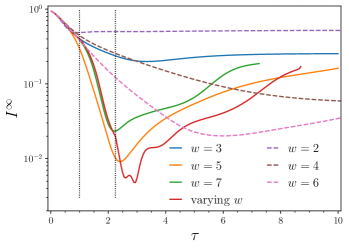
Figure 4: The infidelity with the desired ground state for both the adiabatic QITE and the original QITE algorithm. Even values of $w$ correspond to the original QITE algorithm and the odd $w$ values and the varying case correspond to the adiabatic QITE. The time steps are taken as 0.05 for A-QITE and 0.08 for QITE. The varying $w$ case starts with $w=3$, then changes to $w=5$ and ultimately to $w=7$. The position of the transitions are shown by vertical dotted lines.

We next study $\tilde{H}$ generated by Eq. (6) as a function of system size $L$, and a fixed classical time step $\epsilon=0.05$ in Fig. 2. The results are similar to those using $\tilde{H}$ generated by Eq. (4) if no locality approximation is applied. Examining $I^{\infty},I^{\tau}$, we see the same behaviour of reaching a minimum $I^{\infty}$ and a maximum $I^{\tau}$ at some approximate time $\tau_{c}$. Although $||\tilde{H}||$ grows more quickly and ${\tilde{\Delta}}$ decays more rapidly as $L$ increases, surprisingly, this does not seem to change the maximum reliable propagation time, $\tau_{c}\approx 1.8$, between $L=6-12$.

We further apply the locality heuristic for the generation of $\tilde{H}$, implemented using Eq. (6), in Fig. 3. We use width $w=5$ and a range of system sizes and integration time-steps. Encouragingly, we also see rapid exponential decay of the infidelity to values of $\sim 10^{-2}$ or less. Overall, the dynamics shows similar behaviour to previous examples, and at longer times there is a $\tau_{c}$ corresponding to a change in the behaviour of the infidelities and gaps. However, unlike in the dynamics above without the locality approximation, as the time-step goes to $0$, the minimum $I_{\infty}$ does not keep decreasing, because there is a finite width error.

In Fig. 4, we show $\tilde{H}$ generated by Eq. (6), using the locality heuristic with widths $3,5,7$, and timestep $\epsilon=0.05$, as well as a protocol where the width is increased at increasing times. For comparison, we also show data from the original quantum imaginary time evolution scheme with widths $2,4,6$ and for time step $\epsilon=0.08$. As expected, the best achievable fidelity with the exact state $I^{\infty}(\tau)$ increases with $w$, however, the best $I(\infty)$ in fact decreases moving from $w=5$ to $w=7$. Compared to the original QITE scheme, the achievable infidelity appears to be better (i.e.lower) using the adiabatic Hamiltonian $\tilde{H}$ with a similar locality definition. Further work is required to establish a more precise relationship between these approximations.

We finally consider the modified $\tilde{H}$ generated in a different gauge using Eq. (7). As an illustrative example, we consider the case $u_{1}=1/2$, $u_{2}=2$, with the locality constraint $w=5$. In Fig. 5, we see that although the behaviour of the infidelities $I_{\infty}$ and $I^{\tau}$ are qualitatively similar to what we have seen previously (corresponding to $u_{1}=u_{2}=0$) with a similar $\tau_{c}$, the detailed form is different. For example, the infidelity has a flatter plateau region, and $||H||$ and $\Delta$ show slower growth and flatter decay up to $\tau_{c}$. This indicates that a suitable choice of $f(u)$ can meaningfully modify the dynamics and the achievable infidelities at finite times.

\begin{overpic}[height=177.78578pt]{I_w_5_uful.pdf} \put(5.0,195.0){(a)} \put(5.0,100.0){(b)} \end{overpic}

\begin{overpic}[height=177.78578pt]{Delta_and_Lambda_w_5_uful.pdf} \put(5.0,195.0){(c)} \put(5.0,100.0){(d)} \end{overpic}

Figure 5: Adiabatic evolution under $\tilde{H}$ generated by Eq. (7) with $u_{1}=2,u_{2}=0.5$, block size $w=5$, second-order Runge-Kutta, $\epsilon=0.05$, for the Heisenberg XXZ system for various lengths. Quantities same as in Fig. 1.

IV Conclusions

We have described an adiabatic state preparation protocol that implements the imaginary time evolution trajectory without any need for quantum tomography or ancilla resources. This hybrid algorithm involves a classical time integration to generate the adiabatic Hamiltonian. When implemented faithfully, the algorithm leads to an exponential decrease of the infidelity with the ground-state of a desired Hamiltonian with adiabatic time. However, the cost of evolving exactly to long imaginary times grows rapidly with imaginary time both in the classical and quantum parts of the protocol. The growth in cost as a function of imaginary time arises from several sources, including the nonlocality of the derived adiabatic Hamiltonian. This nonlocality can be controlled by suitable heuristics which truncate terms in the adiabatic Hamiltonian. Another source of growing cost at long imaginary time is related to the norm of the adiabatic Hamiltonian and its gap, for which modifications of the generating equation of the adiabatic Hamiltonian can be introduced and which should be further explored. However, because of the rapid decrease of the infidelity it is possible to propagate for short times and to observe a large improvement in the approximate ground-state. More generally, the A-QITE adiabatic path introduced in this work can be considered as extending the space of possible adiabatic paths; this potentially allows for introduction of new quantum adiabatic routines consisting of composite adiabatic paths (with A-QITE as one of them), with applications such as introduction of novel adiabatic catalysts Albash and Lidar (2018); Farhi et al. (2002), etc. This is a direction to be explored in the future.

Overall, a significant advantage of the current approach is that it can be implemented with a minimal amount of quantum resources (i.e. no ancillae and no measurement-based feedback). This makes our procedure a good match for near-term quantum architectures.

V Acknowledgments

We thank Yu Tong, Alex Dalzell and Anthony Chen for helpful discussions.
KH and GKC were supported by the US Department of Energy, Office of Science, Basic Energy Sciences, under grant no. DE-SC-0019374. GKC acknowledges support from the Simons Foundation.

References

- Preskill (2018) J. Preskill, Quantum 2, 79 (2018).
- Bauer et al. (2020) B. Bauer, S. Bravyi, M. Motta, and G. K.-L. Chan, Chemical Reviews 120, 12685 (2020).
- Peruzzo et al. (2014) A. Peruzzo, J. McClean, P. Shadbolt, M.-H. Yung, X.-Q. Zhou, P. J. Love, A. Aspuru-Guzik, and J. L. O’brien, Nature communications 5, 4213 (2014).
- Farhi et al. (2014) E. Farhi, J. Goldstone, and S. Gutmann, arXiv preprint arXiv:1411.4028 (2014).
- McClean et al. (2016) J. R. McClean, J. Romero, R. Babbush, and A. Aspuru-Guzik, New Journal of Physics 18, 023023 (2016).
- Schön et al. (2007) C. Schön, K. Hammerer, M. M. Wolf, J. I. Cirac, and E. Solano, Physical Review A 75, 032311 (2007).
- Romero et al. (2018) J. Romero, R. Babbush, J. R. McClean, C. Hempel, P. J. Love, and A. Aspuru-Guzik, Quantum Science and Technology 4, 014008 (2018).
- Albash and Lidar (2018) T. Albash and D. A. Lidar, Reviews of Modern Physics 90, 015002 (2018).
- Babbush et al. (2014) R. Babbush, P. J. Love, and A. Aspuru-Guzik, Scientific reports 4, 1 (2014).
- Veis and Pittner (2014) L. Veis and J. Pittner, The Journal of Chemical Physics 140, 214111 (2014).
- Motta et al. (2020) M. Motta, C. Sun, A. T. Tan, M. J. O’Rourke, E. Ye, A. J. Minnich, F. G. Brandão, and G. K. Chan, Nature Physics 16, 205 (2020).
- Sun et al. (2021) S.-N. Sun, M. Motta, R. N. Tazhigulov, A. T. Tan, G. K.-L. Chan, and A. J. Minnich, PRX Quantum 2, 010317 (2021).
- Gomes et al. (2020) N. Gomes, F. Zhang, N. F. Berthusen, C.-Z. Wang, K.-M. Ho, P. P. Orth, and Y. Yao, Journal of Chemical Theory and Computation 16, 6256 (2020).
- Kamakari et al. (2022) H. Kamakari, S.-N. Sun, M. Motta, and A. J. Minnich, PRX Quantum 3, 010320 (2022).
- Yeter-Aydeniz et al. (2022) K. Yeter-Aydeniz, E. Moschandreou, and G. Siopsis, Physical Review A 105, 012412 (2022).
- Farhi et al. (2000) E. Farhi, J. Goldstone, S. Gutmann, and M. Sipser, arXiv preprint quant-ph/0001106 (2000).
- Messiah (2014) A. Messiah, Quantum mechanics (Courier Corporation, 2014).
- McArdle et al. (2019) S. McArdle, T. Jones, S. Endo, Y. Li, S. C. Benjamin, and X. Yuan, npj Quantum Information 5, 75 (2019).
- Kosugi et al. (2022) T. Kosugi, Y. Nishiya, H. Nishi, and Y.-i. Matsushita, Physical Review Research 4, 033121 (2022).
- Note (1) In the same fashion as Ref. Motta et al. (2020), we take the effect of separate terms of into account separately for , so each time step consists of a sequence of substeps, each one propagating for time with a single term of .
- Orbach (1958) R. Orbach, Physical Review 112, 309 (1958).
- Mikeska and Kolezhuk (2004) H.-J. Mikeska and A. K. Kolezhuk, Quantum magnetism , 1 (2004).
- Ding and Lin (2023) Z. Ding and L. Lin, PRX Quantum 4, 020331 (2023).
- Farhi et al. (2002) E. Farhi, J. Goldstone, and S. Gutmann, arXiv preprint quant-ph/0208135 (2002).