Monte Carlo approach to the evaluation of the security of device-independent quantum key distribution
Abstract
We present a generic study on the information-theoretic security of multi-setting device-independent quantum key distribution protocols, i.e., ones that involve more than two measurements (or inputs) for each party to perform, and yield dichotomic results (or outputs). The approach we develop, when applied in protocols with either symmetric or asymmetric Bell experiments, yields nontrivial upper bounds on the secure key rates, along with the detection efficiencies required upon the measuring devices. The results imply that increasing the number of measurements may lower the detection efficiency required by the security criterion. The improvement, however, depends on (i) the choice of multi-setting Bell inequalities chosen to be tested in a protocol, and (ii) either a symmetric or asymmetric Bell experiment is considered. Our results serve as an advance toward the quest for evaluating security and reducing efficiency requirement of applying device-independent quantum key distribution in scenarios without heralding.
I Introduction
Device-independent quantum key distribution (DIQKD) Ekert91 ; MY98 ; BHK05 ; AGM06 ; AMP06 ; ABG+07 ; PAB+09 ; PAM+10 ; MPA11 ; AMP12 ; TH13 ; VV14 ; MS16 ; A-FDF+18 ; A-FRV19 ; MvDR+19 requires minimal assumptions on implementation devices to certify an information-theoretic security, thus serving as one of promising ways to ruling out side-channel attacks and narrowing the ideal-versus-practical gap in security. It involves Bell tests (BT) BCP+14 accomplished in a loophole-free manner HBD+15 ; GVW+15 ; SM-SC+15 ; RBG+17 ; LWZ+18 , to quantitatively evaluate eavesdropping by some potential adversary, Eve. Both DIQKD and BT, however, suffer compromised consequences without closing the loopholes Bell04 ; Pearle70 ; CH74 ; GG99 . To the end, one approach, among others, to closing the detection loophole, one of the principal loopholes in BT, resorts to increasing the number of measurements Massar02 ; MPR+02 ; MP03 ; BG08 ; PV09 ; VPB10 ; Branciard11 . It has been estimated that performing more measurements in each party may provide improvement in decreasing the threshold efficiency. Namely, one can have MP03 , where are the numbers of measurements (settings) of the two parties, Alice and Bob. One then is led to be expecting that, to get shared secure keys, increasing the number of measurements in DIQKD, where the detection loophole is more serious than in BT, may stand to benefit from the decrease of the threshold efficiency in BT.
Several difficulties with investigating multi-setting DIQKD protocols arise and—in spite of a few case studies—remain. First, the general quantity for efficiencies in MP03 represents a lower bound; whether it can always be reached, or to what extent it can be adapted to cryptographic protocols, is yet to be conclusive. Second, due to the particular structure of the Clauser-Horne-Shimony-Holt (CHSH) inequality Bell64 ; CHS+69 , it suffices to consider a -dimensional Hilbert subspace in the security analysis of the CHSH-based protocol ABG+07 ; PAB+09 . Multi-setting protocols do not share such a mathematical structure, rendering the security analysis all the more complicated. In fact, without affecting the faithfulness in experiment, there have been a number of methods to improving the efficiencies by having undesired data deducted. For instance, one can use the heralding method (see, e.g., ZLA-F+23 for the concepts and references therein; also XMZ+20 ; PR22 ; PGT+23 ), e.g., via the non-destructive detection NFL+21 or the qubit amplifiers ZC19 ; GPS10 ; PMW+11 ; CM11 ; M-SBB+13 ; KMS+20 , to select signals to trigger detection, while safely neglecting undetected events; or, one can perform a classical data post-processing scheme for the error-correction purpose to improve the key rates ML12 .
Without heralding, to reduce the efficiency requirement in DIQKD still remains an important question. The following two efficiencies of measuring devices are often the cases in practice BGS+07 :
where are efficiencies of Alice’s and Bob’s measuring devices, respectively. The symmetric case denotes equally non-ideal measurements by Alice and Bob when the information carriers are of the same type of particles (e.g., entangled photon pairs); the asymmetric case denotes ideal-versus-non-ideal measurements when they are not of the same type of particles (e.g., entangled atom-photon pairs BMD+04 ; MMB+04 ; VWS+06 with which Alice measures the atoms and Bob measures the photons). In general, it is a simple way to come up with a DIQKD protocol out of the BT by adding to Bob one more measurement which coincides with one of Alice’s measurements along, say, the -axis, and using this pair of measurements to generate keys.
In this paper, we develop a Monte Carlo approach to evaluating upper bounds on the secure key rates in multi-setting two-output DIQKD protocols against collective attacks. We consider both symmetric and asymmetric detection setups in BT and key generation. The threshold efficiency of the CHSH-based protocol is found to be approximately in the asymmetric setup, less than the well-known in the symmetric setup PAB+09 . The threshold efficiency of the -based protocol is estimated to be approximately in the asymmetric setup, as well as those of a large family of multi-setting-inequality-based protocols being estimated to be less than , too. A remark here is that it is the modeling of undetected events presented in PAB+09 that we take to use in this paper to evaluate the eavesdropping information. There have been literatures wherein different modelings are used (for instance, see BFF21 ; WAP21 ; BFF21-2 ; MPW22 ; LB-JF+22 for recent methods to evaluating the eavesdropping). In general, taking account of more input-output statistics of undetected events, e.g., adding one more output to each party to register the undetected event, may yield slightly higher key rates. The key rates can be further improved by considering partially entangled states and noisy-preprocessing techniques (see, e.g., LB-JF+22 ), thus the resulting threshold efficiencies may be improved as well.
The paper is structured as follows. We first describe the general setup for DIQKD protocols with undetected events taken into account. We then present the evaluation of key rates by developing a formalism in which the mutual information and eavesdropping information are put in a same index. It is followed by an explicit procedure of a Monte Carlo approach, along with case studies of the CHSH- and -based CG04 protocols and the BB84-type protocol BB84 . The efficiencies and critical error rates are estimated with Bell diagonal states. More protocols with other multi-setting Bell inequalities are also studied. We proceed beyond the -dimensional subspaces and generalize the Monte Carlo approach to arbitrarily high-dimensional systems. The paper ends with a summary and outlook.
II Security of multi-setting quantum key distribution
II.1 General setup
Let us assume the measurements used in the security proof be projective ones. To justify the use, note that if one uses the positive-operator-valued measures (POVMs) to perform measurements, they can readily be transformed to projectors by the Naimark theorem. Obviously, projective measurements become POVMs when undetected events are taken into account (see, e.g., Eq. (4) below ). In general scenarios, the projectors are not necessary to be of rank one. By requiring that measurement must produce, for instance, two distinct outcomes, the projectors could be of rank two or higher (see, e.g., Eq. (23) below).
Consider bipartite Hilbert spaces of dimension and a measurement set . Given projectors
| (1) |
respectively for Alice and Bob, the joint correlation is computed as quantum mechanically, where Alice chooses her -th measurement, getting result , Bob chooses his -th measurement, getting result , denotes the state shared by Alice and Bob, and are unitary transformations in group. Let us tacitly assume, when take unit identity , that one can have and where span a set of computational bases.
An -setting -dimensional Bell inequality, denoted by , can be expressed as
| (2) |
with ’s coefficients properly chosen to make the inequality nontrivial, i.e., violated in quantum mechanics. The inequality holds for all local-hidden variable models Bell64 . Let us denote quantum violation as
| (3) |
with respect to some . It should be noted that a large family of Bell inequalities reach their maximum quantum violations under very particular sets of measurements (e.g., Bell multi-port measurements ZZH97 ) but for the sake of generality we maintain as arbitrary unitary transformations.
To model undetected events in experiment outputting dichotomic results and , let us assign the undetected with , and so with an detection efficiency the projectors become non-ideal, reading actually
| (4) |
with . The term is due to the undetected events and , both of which happen with probability and according to the model should then be assigned , contributing to the actual . Applying (4) to joint correlations of Alice and Bob yields (see also G-UPC21 )
| (5) |
where denotes the Kronecker function, and are marginals.
II.2 Evaluation of key rates
We choose to take the information-theoretic key rate to analyze the security. One needs to first evaluate the eavesdropping information and the mutual information , and then attain in the infinite-length limit the key rate DW05 . Let us stress, however, that the use of Bell diagonal states in what follows is a strong assumption on the security, and that in our approach finding optimal states that maximize Eve’s information may not be guaranteed for more-than-two-input scenarios in general. Hence the ’s evaluated below serves as upper bounds on the key rates.
To compute , one needs to optimize the Holevo quantity , where is the von Neumann entropy, denotes Eve’s reduced state, and denotes Eve’s normalized conditional state upon Alice’s measurement . Since there exists an overall distilled pure state from which and can be attained in a reduction way, one has . The fact that instead of all possible bipartite states it suffices to consider the Bell-diagonal state ABG+07 ; PAB+09 , reading with , , , , and , leads to .
To get further simplification, note that is of rank two, with eigenvalues (which are derived in the -plane in PAB+09 ; see also Su22 )
| (6) |
with respect to Alice’s measurements , where , , and
| (7) |
With all these combined, the Holevo quantity becomes , with the classical Shannon entropy and the binary entropy .
Because the measurements may not be faithfully performed, the Holevo quantity should be presumed to be maximized, or equivalently, taking into account the monotonicity of , the (or ) should be presume to be minimized (or maximized). Let
| (8) |
and we find
| (9) |
It follows that has three extrema:
| (10) |
where
| (11) |
Let be the set of all parameters in Bell-diagonal states, and be a subset that corresponds to some particular value of quantum violation . The eavesdropping information is found to be
| (12) |
In other words, one can thus have a -dependent .
To compute , one needs first to get the quantum bit error rate (QBER) . Taking undetected events into account, it becomes
| (13) |
with for the Bell-diagonal state. It is well acceptable that one can assume due to the preparation of states in practice, getting the QBER equal in the - and -axes. Hence one gets the mutual entropy . Despite that the , or , in general, is irrelevant to , it is vital in our approach that one must define a -dependent mutual information, in order to evaluate the key rate.
To the end, let be a subset that corresponds to some particular value of mutual entropy . As such, the states in will yield a domain of quantum violation, namely,
| (14) |
Then some must exist in the domain such that reaches a local maximum:
| (15) |
For all pairs , there must be a mapping, namely,
| (16) |
which can thus be used as a -dependent .
It is here remarked, for one thing, that in computing , non-ideal efficiencies (i.e., undetected events) should be taken into account; but in computing the efficiencies should be presumed ideal, because Eve gets the most information when Alice faithfully performs measurements in order to try with Bob to generate keys. For another, as derived above, one can have both and dependent on ; however, the state that yields is not required to be the same as the state that yields . If, instead, one requires the states that yield to be the same in computing and , as well as specifying Alice’s measurements in evaluating Eve’s conditional states (i.e., replacing the maximization (12) with a Holevo quantity that corresponds to that Alice always measuring along the -axis), then the protocol reduces to a BB84 protocol in which the device-independent feature is lost (see the example below; also ABG+07 ; PAB+09 ).
II.3 Procedure of the Monte Carlo approach
The procedure is summarized in Table. 1. Once the key rate is attained, it is immediate to derive a number of critical values, e.g., the maximum QBER and the threshold efficiency for a selected protocol.
| Steps | Descriptions for each step |
|---|---|
| 1 | Select a DIQKD protocol in which the Bell test and key generation are specified. |
| 2 | Randomly generate a Bell-diagonal state and compute the Holevo quantity . |
| 3 | Compute the quantum violation of the Bell inequality with . |
| 4 | Record the pair . |
| 5 | Repeat steps 1 through 4 sufficiently many times to collect the data of pairs , the upper bound of which corresponds then to the eavesdropping information . |
| 6 | Randomly generate a Bell-diagonal state and compute the QBER , from which to get the mutual entropy . |
| 7 | Compute the quantum violation of the Bell inequality with . |
| 8 | Record the pair . |
| 9 | Repeat steps 6 through 8 sufficiently many times to collect the data of pairs , from which, together with the definition (16), one can determine the mutual information . |
| 10 | Evaluate the key rate with respect to any . |
II.4 Case studies
We illustrate our approach in two examples, alongside a reduction to the BB84 protocol.
II.4.1 The CHSH-based protocol
It suffices here to consider Bell-diagonal states, since it has been proved that dimensional subspaces can always be found in evaluating the key rate for any two-input-two-output scenarios PAB+09 . The CHSH inequality reads (which is actually the Clauser-Horne inequality CH74 in mathematical equivalence), with short notations , , and .
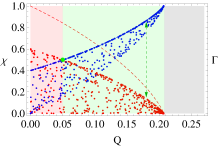
Following the Monte Carlo procedure, we pin down and , as shown in Figs. 1(a) through 1(d). The argument is as follows. First, it is immediate to see from the figure that for each there corresponds to non-unique , and the serves as the upper bound. Then, for each there corresponds to non-unique and, according to the definition (16), the should be taken at a value of at which reaches a local maximum. In the CHSH case, always decreases with the increase of , meaning that for each , it is the that yields a maximum . The is henceforth pinned down.
The critical QBER corresponds to the cross point
| (17) |
from which we find . The threshold efficiency can be attained when there is no legitimate data of above the curve any more. Here, we find and for symmetric and asymmetric Bell experiments, respectively.
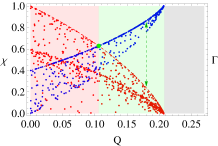
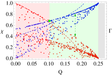
Obviously, the curves in Fig. 1 match the analytic results derived in ABG+07 ; PAB+09 ; namely, the eavesdropping information
| (18) |
and, with the QBER associated with , the mutual information
| (19) |
The critical QBER and threshold efficiency can then be verified by letting . As mentioned in Introduction, if one adds one more output to register the undetected events, the input-output statistics with maximally entangled states can yield a slightly lower threshold efficiency down to approximately WAP21 , and via the convex-combination method LB-JF+22 an efficient upper bound on the key rate implies a threshold efficiency as approximately .
II.4.2 The -based protocol
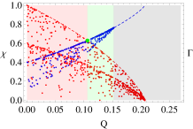
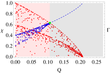
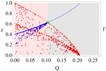
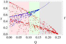
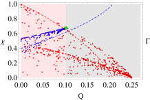
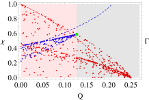
For multi-input-two-output scenarios there is in general no nontrivial low-dimensional subspaces, the key rate evaluated with Bell-diagonal states is actually an estimated one. The inequality reads CG04 , with the same short notations as in the CHSH inequality. Again, we pin down and , shown in Figs. 1(e) through 1(h), with a very similar argument.
A distinct feature appears in the scenario, however. Note that the cross point varies with respect to efficiency. For instance, in the asymmetric setup, one can get
| (20) |
as , yielding ; and
| (21) |
as , yielding . Along with an advantage over the threshold efficiency, i.e., here for the case versus for the CHSH case, it is shown that in DIQKD protocols the inequality seems more suitable than the CHSH inequality in the asymmetric setup, just as it indeed is in asymmetric BT BGS+07 . It is henceforth implied that more measurements may indeed have distinct merits in asymmetric DIQKD.
Shown in Table 2 are results with various other Bell inequalities. These inequalities reach quantum maxima with the maximally entangled state BG08 . The explicit expressions of the inequalities are shown in Table 3. In LB-JF+22 , a couple of multi-setting protocols proposed in G-UPC21 are studied via the convex-combination method. Therein the threshold efficiencies are shown to be improved. Nevertheless, one protocol there involves a more-than-two-output Bell inequality and the other protocol there involves a Bell inequality whose violation requires high-dimensional quantum states. We have not studied the two protocols due to scope issues.
| CHSH | 0.0715 | 0.0715 | 0.0715 | 0.924 | 0.858 |
|---|---|---|---|---|---|
| 0.0586 | 0.0586 | 0.0822 | 0.938 | 0.836 | |
| 0.0586 | 0.0552 | 0.0586 | 0.942 | 0.880 | |
| 0.0532 | 0.0417 | 0.0426 | 0.957 | 0.916 | |
| 0.0663 | 0.0663 | 0.0663 | 0.927 | 0.864 | |
| 0.0698 | 0.0698 | 0.0698 | 0.924 | 0.858 | |
| 0.0679 | 0.0637 | 0.0537 | 0.932 | 0.893 | |
| 0.0591 | 0.0559 | 0.0532 | 0.942 | 0.895 | |
| 0.0532 | 0.0480 | 0.0433 | 0.950 | 0.915 | |
| 0.0462 | 0.0501 | 0.0499 | 0.947 | 0.900 | |
| 0.0473 | 0.0417 | 0.0428 | 0.955 | 0.915 | |
| 0.0485 | 0.0485 | 0.0485 | 0.950 | 0.905 |
II.4.3 Reduction to the BB84 protocol
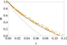
As the aforementioned, the DIQKD protocol will reduce to the BB84 protocol if one specifies Alice’s measurements. In Fig. 2, it is shown that in each step one randomly selects a Bell-diagonal state from which to get the pair and the pair, where is attained by fixing Alice’s measurements in evaluating along the -axis. The Monte Carlo procedure then yields the mutual and eavesdropping information as in the BB84 protocol. Note that the cross point leads to the well-known critical QBER .
| Expressions for each Bell inequality | |
|---|---|
| CHSH | |
II.5 Beyond subspaces
To have more precise estimates of the key rate, i.e., to lower the upper bounds obtained in subspaces, one is required to consider arbitrarily high dimensional Hilbert spaces producing dichotomic outputs under unfaithful measurements with non-ideal efficiencies. It is then straightforward to generalize the Monte Carlo procedure in Table 1 to make it work for high dimensions. The steps are similar as those in Table 1, except for a few quantities which must be adapted for high-dimensional states. The relevant equations are listed below.
| (22) | |||
| (23) | |||
| (24) | |||
| (25) | |||
| (26) | |||
| (27) | |||
| (28) | |||
| (29) | |||
| (30) | |||
| (31) | |||
| (32) |
We would like to elaborate now. Some steps in Table 1 remain unchanged, except the following ones. For step 2, one needs to consider a high-dimensional state . The coefficients must satisfy constraints such that the generated key, obtained by measurements in the basis of key generation, is random. A possible example could be , with . Due to the two-output feature of the protocol, some measuring results for the key should be denoted as 0 and the others as 1 (indexed by in (22); see the remarks below for detail). Other examples could be , , etc., or their convex combinations. The Holevo quantity can then be computed via (29).
For step 3, to compute of a two-output Bell inequality , the projectors with respect to a certain are constructed in (23). With the above high-dimensional , one can have the quantum violation, i.e., (24). For step 5, the eavesdropping information is attained in (30) by numerating all possible ’s. The constraints correspond to the requirement of randomness upon the key.
For steps 6 and 7, similarly, one considers a high-dimensional and compute the error rate in (25) from which to get the mutual entropy under non-ideal efficiencies, i.e., (27). The quantum violation is computed with . After collecting sufficient data, one can have the mutual information (31) in step 9.
Finally, for step 10, one have attained a set of key rates (32) with various ’s and ’s. An efficient upper bound of the key rate in the protocol is then taken as the minimum.
Further remarks are in order. First, equations (22)-(23) are defined so because the dimensions of the systems used should be presumed unknown while in measurements dichotomic results should always be attained. One thus needs to numerate all possible divisions, here indicated by ’s, each of which denotes that the first dimensions yield result and the remaining dimensions yield result (or equivalently, through(23), the first dimensions yield result and the remaining dimensions yield result ). The divisions have included all possible reordering of results since swap operations are among the unitary transformations. Bell inequalities of probabilistic form , because of (23), can be equivalent to inequalities of correlation form in which measurements of each party produce . For instance, the inequality holds quantum mechanically with any -dimensional entangled states but can be violated with a - or -dimensional entangled state. Going beyond the -dimensional subspaces in the security analysis is henceforth very nontrivial (see also G-UPC21 ).
Second, it is similar, as with the subspaces, to model undetected events and to compute the error rates and mutual entropy, which are all associated with outputs . In computing the Holevo quantity, however, it is essential to distinguish each dimension, in order to have the eavesdropping maximized whereby to pin down the . In analogy to considering Bell-diagonal states and in the previous section, the in (31) represents a set of high-dimensional states shared between Alice and Bob and the represents a subset of that leads to some particular in the BT, with the parameters in the state in analogy to in Bell-diagonal states. After pinning down a -dependent in (31), which follows the definition (16), one can get a provisional upper bound on the key rate with respect to certain and .
III Summary and outlook
We have presented a Monte Carlo approach to evaluating information-theoretic security of DIQKD protocols. We have been able to asymptotically compute the key rates with the eavesdropping information and mutual information in terms of a same index, i.e., the , via associating the QBER of the key with quantum violation of the Bell inequality. From the key rates, the critical QBERs and efficiencies of a family of protocols have been evaluated. The approach not only applies to scenarios with extremal efficiencies as in our case studies but also to those with general ones, and can subsequently be extended to multi-output protocols. Our results show that in either the symmetric or the asymmetric setup of the protocols not so many established multi-setting Bell inequalities, except for the inequality so far among the family of inequalities we have considered, have better performance than the CHSH inequality. Hence it is a nontrivial task that one needs to select or build Bell inequalities for multi-setting protocols. The merits of the approach include: (i) the procedure is quite efficient, as it can reproduce the exact key rate in the CHSH-based protocol, while in general protocols it yields upper bounds on the key rates, and (ii) the asymmetric setups are closer to practical scenarios, since the nodes in a quantum network, for instance, usually have unequal detection efficiencies.
A couple of open questions remain. In our case studies, the eavesdropping information decreases as quantum violation increases; hence always the upper bound of mutual entropy should the mutual information correspond to. It remains an open question, then, of whether there are any counterexamples where takes reversed monotonicity; we conjecture there might be in protocols with more-than-two outputs. One more question is whether there are quantum algorithms to speed up the matrix diagonalization in evaluating the Holevo quantity for large .
Acknowledgements.
The author is grateful to Professor W.-Y. Hwang for enlightening the heralding method in DIQKD and BT, and the anonymous referees for giving very constructive comments. The study is supported by the National Natural Science Foundation of China (Grant No. 11905209) and the Fundamental Research Funds for the Central Universities (Grant No. 3072022TS2503).References
- (1) Ekert A K 1991 Quantum cryptography based on Bell’s Theorem Phys. Rev. Lett. 67 661
- (2) Mayers D and Yao A Quantum cryptography with imperfect apparatus In Proceedings 39th Annual Symposium on Foundations of Computer Science 503-509 (IEEE, 1998)
- (3) Barrett J, Hardy L and Kent A 2005 No signaling and quantum key distribution Phys. Rev. Lett. 95 010503
- (4) Acín A, Gisin N and Masanes L 2006 From Bell’s theorem to secure quantum key distribution Phys. Rev. Lett. 97 120405
- (5) Acín A, Massar S and Pironio S 2006 Efficient quantum key distribution secure against no-signalling eavesdroppers New J. Phys. 8 126
- (6) Acín A, Brunner N, Gisin N, Massar S, Pironio S and Scarani V 2007 Device-independent security of quantum cryptography against collective attacks Phys. Rev. Lett. 98 230501
- (7) Pironio S, Acín A, Brunner N, Gisin N, Massar S and Scarani V 2009 Device-independent quantum key distribution secure against collective attacks New J. Phys. 11 045021
- (8) Pironio S, Acín A, Massar S, Boyer de la Giroday A, Matsukevich D N, Maunz P, Olmschenk S, Hayes D, Luo L, Manning T A and Monroe C 2010 Random numbers certified by Bell’s theorem Nature 464 1021-1024
- (9) Masanes L, Pironio S and Acín A 2011 Secure device-independent quantum key distribution with causally independent measurement devices Nat. Commun. 2 1-7
- (10) Acín A, Massar S and Pironio S 2012 Randomness versus nonlocality and entanglement Phys. Rev. Lett. 108 100402
- (11) Tomamichel M and Häggi E 2013 The link between entropic uncertainty and nonlocality J. Phys. A: Math. Theor. 46 055301
- (12) Vazirani U and Vidick T 2014 Fully device-independent quantum key distribution Phys. Rev. Lett. 113 140501
- (13) Miller C A and Shi Y 2016 Robust protocols for securely expanding randomness and distributing keys using untrusted quantum devices J. ACM 63 1-63
- (14) Arnon-Friedman R, Dupuis F, Fawzi O, Renner R and Vidick T 2018 Practical device-independent quantum cryptography via entropy accumulation Nat. Commun. 9 1-11
- (15) Arnon-Friedman R, Renner R and Vidick T 2019 Simple and tight device-independent security proofs SIAM J. Comput. 48 181-225
- (16) Murta G, van Dam S B, Ribeiro J, Hanson R and Wehner S 2019 Towards a realization of device-independent quantum key distribution Quantum Sci. Technol. 4 035011
- (17) Brunner N, Cavalcanti D, Pironio S, Scarani V and Wehner S 2014 Bell nonlocality Rev. Mod. Phys. 86 419
- (18) Hensen B, Bernien H, Dréau A E, Reiserer A, Kalb N, Blok M S, Ruitenberg J, Vermeulen R F L, Schouten R N, Abellán C, Amaya W, Pruneri V, Mitchell M W, Markham M, Twitchen D J, Elkouss D, Wehner S, Taminiau T H and Hanson R 2015 Loophole-free Bell inequality violation using electron spins separated by 1.3 kilometres Nature 526 682-686
- (19) Giustina M, Versteegh M A M, Wengerowsky S, Handsteiner J, Hochrainer A, Phelan K, Steinlechner F, Kofler J, Larsson J-A, Abellán C, Amaya W, Pruneri V, Mitchell M W, Beyer J, Gerrits T, Lita A E, Shalm L K, Nam S W, Scheidl T, Ursin R, Wittmann B and Zeilinger A 2015 Significant-loophole-free test of Bell’s theorem with entangled photons Phys. Rev. Lett. 115 250401
- (20) Shalm L K, Giustina M, Meyer-Scott E, Christensen B G, Bierhorst P, Wayne M A, Stevens M J, Gerrits T, Glancy S, Hamel D R, Allman M S, Coakley K J, Dyer S D, Hodge C, Lita A E, Verma V B, Lambrocco C, Tortorici E, Migdall A L, Zhang Y, Kumor D R, Farr W H, Marsili F, Shaw M D, Stern J A, Abellán C, Amaya W, Pruneri V, Jennewein T, Mitchell M W, Kwiat P G, Bienfang J C, Mirin R P, Knill E and Nam S W 2015 Strong loophole-free test of local realism Phys. Rev. Lett. 115 250402
- (21) Rosenfeld W, Burchardt D, Garthoff R, Redeker K, Ortegel N, Rau M and Weinfurter H 2017 Event-ready Bell test using entangled atoms simultaneously closing detection and locality loopholes Phys. Rev. Lett. 119 010402
- (22) Li M-H, Wu C, Zhang Y, Liu W-Z, Bai B, Liu Y, Zhang W, Zhao Q, Li H, Wang Z, You L, Munro W J, Yin J, Zhang J, Peng C-Z, Ma X, Zhang Q, Fan J and Pan J-W 2018 Test of local realism into the past without detection and locality loopholes Phys. Rev. Lett. 121 080404
- (23) Bell J S In Speakable and unspeakable in quantum mechanics (Cambridge University Press, 2004) chap. 24.
- (24) Pearle P M 1970 Hidden-variable example based upon data rejection Phys. Rev. D. 2 1418
- (25) Clauser J F and Horne M A 1974 Experimental consequences of objective local theories Phys. Rev. D. 10 526
- (26) Gisin N and Gisin B 1999 A local hidden variable model of quantum correlation exploiting the detection loophole Phys. Lett. A 260 323-327
- (27) Massar S 2002 Nonlocality, closing the detection loophole, and communication complexity Phys. Rev. A 65 032121
- (28) Massar S, Pironio S, Roland J and Gisin B 2002 Bell inequalities resistant to detector inefficiency Phys. Rev. A 66 052112
- (29) Massar S and Pironio S 2003 Violation of local realism versus detection efficiency Phys. Rev. A 68 062109
- (30) Brunner N and Gisin N 2008 Partial list of bipartite Bell inequalities with four binary settings Phys. Lett. A 372 3162-3167
- (31) Pál K F and Vértesi T 2009 Quantum bounds on Bell inequalities Phys. Rev. A 79 022120
- (32) Vértesi T, Pironio S and Brunner N 2010 Closing the Detection Loophole in Bell Experiments Using Qudits Phys. Rev. Lett. 104 060401
- (33) Branciard C 2011 Detection loophole in Bell experiments: How postselection modifies the requirements to observe nonlocality Phys. Rev. A 83 032123
- (34) Bell J S 1964 On the Einstein-Podolsky-Rosen paradox Phys. Phys. Fiz. 1 195
- (35) Clauser J F, Horne M A, Shimony A and Holt R A 1969 Proposed experiment to test local hidden-variable theories Phys. Rev. Lett. 23 880
- (36) Zapatero V, van Leent T, Arnon-Friedman R, Liu W-Z, Zhang Q, Weinfurter H and Curty M 2023 Advances in device-independent quantum key distribution npj Quantum Inf. 9 10
- (37) Xu F, Ma X, Zhang Q, Lo H-K and Pan J-W 2020 Secure quantum key distribution with realistic devices Rev. Mod. Phys. 92 025002
- (38) Portmann C and Renner R 2022 Security in quantum cryptography. Rev. Mod. Phys. 94 025008
- (39) Primaatmaja I W, Goh K T, Tan E Y-Z, Khoo J T-F, Ghorai S and Lim C C-W 2023 Security of device-independent quantum key distribution protocols: a review Quantum 7 932
- (40) Niemietz D, Farrera P, Langenfeld S and Rempe G 2021 Nondestructive detection of photonic qubits Nature 591 570-574
- (41) Zapatero V and Curty M 2019 Long-distance device-independent quantum key distribution Sci. Rep. 9 1-18
- (42) Gisin N, Pironio S and Sangouard N 2010 Proposal for implementing deviceindependent quantum key distribution based on a heralded qubit amplifier Phys. Rev. Lett. 105 070501
- (43) Pitkanen D, Ma X, Wickert R, van Loock P and Lütkenhaus N 2011 Efficient heralding of photonic qubits with applications to device-independent quantum key distribution Phys. Rev. A 84 022325
- (44) Curty M and Moroder T 2011 Heralded-qubit amplifiers for practical deviceindependent quantum key distribution Phys. Rev. A 84 010304R
- (45) Meyer-Scott E, Bula M, Bartkiewicz K, Černoch A, Soubusta J, Jennewein T and Lemr K 2013 Entanglement-based linear-optical qubit amplifier Phys. Rev. A 88 012327
- (46) Kołodyński J, Máttar A, Skrzypczyk P, Woodhead E, Cavalcanti D, Banaszek K and Acín A 2020 Device-independent quantum key distribution with singlephoton sources Quantum 4 260
- (47) Ma X and Lükenhaus N 2012 Improved Data Post-Processing in Quantum Key Distribution and Application to Loss Thresholds in Device Independent QKD Quantum Inf. Comput. 12 0203-0214
- (48) Brunner N, Gisin N, Scarani V and Simon C 2007 Detection Loophole in Asymmetric Bell Experiments Phys. Rev. Lett. 98 220403
- (49) Blinov B B, Moehring D L, Duan L-M and Monroe C 2004 Observation of entanglement between a single trapped atom and a single photon Nature 428 153
- (50) Moehring D L, Madsen M J, Blinov B B and Monroe C 2004 Experimental Bell Inequality Violation with an Atom and a Photon Phys. Rev. Lett. 93 090410
- (51) Volz J, Weber M, Schlenk D, Rosenfeld W, Vrana J, Saucke K, Kurtsiefer C and Weinfurter H 2006 Observation of Entanglement of a Single Photon with a Trapped Atom Phys. Rev. Lett. 96 030404
- (52) Brown P, Fawzi H and Fawzi O 2021 Device-independent lower bounds on the conditional von Neumann entropy arXiv:2106.13692
- (53) Woodhead E, Acín A and Pironio S 2021 Device-independent quantum key distribution with asymmetric CHSH inequalities Quantum 5 443
- (54) Brown P, Fawzi H and Fawzi O 2021 Computing conditional entropies for quantum correlations Nature Communications 12 575
- (55) Masini M, Pironio S and Woodhead E 2022 Simple and practical DIQKD security analysis via BB84-type uncertainty relations and Pauli correlation constraints Quantum 6 843
- (56) Łukanowski K, Balanzó-Juandó M, Farkas M, Acín A and Kołodyński J 2022 Upper bounds on key rates in device-independent quantum key distribution based on convex-combination attacks arXiv:2206.06245
- (57) Collins D and Gisin N 2004 A relevant two qubit Bell inequality inequivalent to the CHSH inequality J. Phys. A: Math. Theor. 37 1775
- (58) Bennett C H and Brassard G Quantum cryptography: Public key distribution and coin tossing. in Proceedings IEEE International Conference on Computers, Systems and Signal Processing, Bangalore, India, 1984 (IEEE, New York, 1984), pp. 175-179
- (59) Zukowski M, Zeilinger A and Horne M A 1997 Realizable higher-dimensional two-particle entanglements via multiport beam splitters Phys. Rev. A 55 2564
- (60) Gonzales-Ureta J R, Predojević A and Cabello A 2021 Device-independent quantum key distribution based on Bell inequalities with more than two inputs and two outputs Phys. Rev. A 103 052436
- (61) Devetak I and Winter A 2005 Distillation of secret key and entanglement from quantum states Proc. R. Soc. A 461 207-235
- (62) Su H-Y 2022 A simple relation of guessing probability in quantum key distribution New J. Phys. 24 093016