Brighten-and-Colorize: A Decoupled Network for Customized Low-Light Image Enhancement

Abstract.

Low-Light Image Enhancement (LLIE) aims to improve the perceptual quality of an image captured in low-light conditions. Generally, a low-light image can be divided into lightness and chrominance components. Recent advances in this area mainly focus on the refinement of the lightness, while ignoring the role of chrominance. It easily leads to chromatic aberration and, to some extent, limits the diverse applications of chrominance in customized LLIE. In this work, a “brighten-and-colorize” network (called BCNet), which introduces image colorization to LLIE, is proposed to address the above issues. BCNet can accomplish LLIE with accurate color and simultaneously enables customized enhancement with varying saturations and color styles based on user preferences. Specifically, BCNet regards LLIE as a multi-task learning problem: brightening and colorization. The brightening sub-task aligns with other conventional LLIE methods to get a well-lit lightness. The colorization sub-task is accomplished by regarding the chrominance of the low-light image as color guidance like the user-guide image colorization. Upon completion of model training, the color guidance (i.e., input low-light chrominance) can be simply manipulated by users to acquire customized results. This customized process is optional and, due to its decoupled nature, does not compromise the structural and detailed information of lightness. Extensive experiments on the commonly used LLIE datasets show that the proposed method achieves both State-Of-The-Art (SOTA) performance and user-friendly customization.

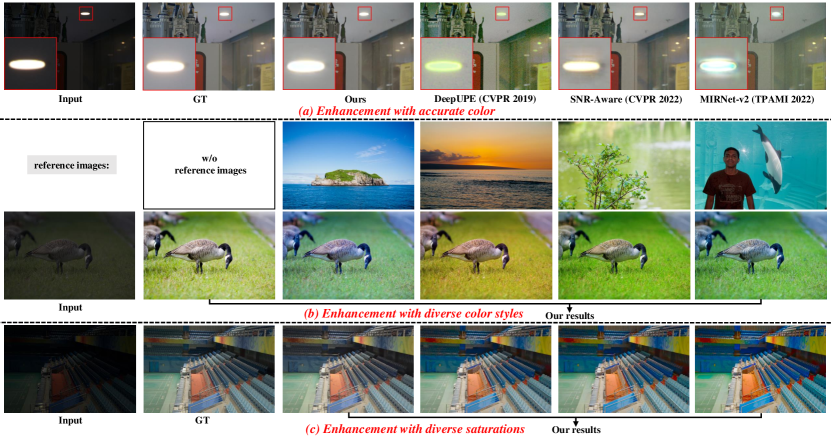
Figure 1. The enhanced results of the proposed method. (a) Compared with the results of current methods (Wang et al., 2019; Xu et al., 2022; Zamir et al., 2022), which suffer from chromatic aberration, the proposed method reaches enhancement with accurate color. (b) The proposed method achieves customized enhancement based on reference images. (c) The proposed method can adjust the saturations of the enhanced results.

1. Introduction

Low-Light Image Enhancement (LLIE) is an important but challenging task in computer vision. It can not only improve the visual quality, but also be helpful for other high-level computer vision tasks (e.g., face detection (Yang et al., 2019), action recognition (Pan et al., 2021), and object detection (Ren et al., 2015)). Until now, many traditional methods (Pizer et al., 1987; Jobson et al., 1997; Rahman et al., 2004) and learning-based methods (Zhang et al., 2019; Lore et al., 2017; Xu et al., 2022; Zamir et al., 2022, 2020; Zhang et al., 2021b; Wang et al., 2019; Yang et al., 2021; Wei et al., 2018) have been proposed to enhance low-light images. However, most of them mainly focus on improving the quality of the lightness, which easily leads to serious loss of chrominance information and unpleasant visual results. Although some works try to apply additional constraints on chrominance information (e.g., the vectors of RGB channels (Wang et al., 2019)), they still hardly handle chrominance information well (as shown in Fig. 1 (a)). On the other hand, chrominance plays an important role in customized enhancement, however, recent customized methods (Zhang et al., 2021a; Kim et al., 2020b; Sun et al., 2021; Zheng et al., 2022; Wang et al., 2022) do not notice this problem. iUP-Enhancer (Zheng et al., 2022) achieved chrominance customization by leveraging histograms in HSV color space, while the histograms as global information hardly guarantee local consistency. In summary, existing (customized) LLIE methods do not pay enough attention to the importance of chrominance information.

Meanwhile, image colorization, as an active research field that aims to predict lost chrominance information on the given lightness, has two key challenges: 1) how to ensure boundaries of the generated chrominance, 2) how to solve the problem that one object can be filled by multiple colors (e.g., a balloon can be colorized red or blue). Some image colorization methods tackle these problems by introducing semantic information (Zhao et al., 2020; Su et al., 2020), which can provide the boundaries or object information, and the user interactions (e.g. color strokes (Zhang et al., 2017) or reference image (He et al., 2018; Lu et al., 2020)), which are helpful for generating the certain colors. However, we observe that although the chrominance of low-light image is unsaturated, it contains both boundary information and some color hints.

Hence, we novelly propose to regard the chrominance prediction in LLIE as a colorization problem, which takes the low-light chrominance as a guidance to recover proper colors. In this way, LLIE is decoupled into the brightening and colorization sub-tasks. Since the input of the colorization process is usually carried out on grey images under normal light, an intuitive implementation is to first brighten the low-light lightness and then colorize it. However, this two-step approach is tedious and lacks information interactions between two sub-tasks. In this work, a new “brighten-and-colorize” paradigm, called BCNet is proposed. BCNet adopts multi-task learning architecture, which contains one encoder and two task-specific decoders. The encoder takes the low-light lightness as the input, while the two task-specific decoders aim to output predicted lightness and chrominance, respectively. By training two sub-tasks simultaneously, the brightening sub-task can provide information of normal-light lightness to the colorization sub-task. Besides, the color classification loss (Zhang et al., 2016), which transforms colorization to a classification task, is introduced to relieve color vanishment in the colorization sub-task.

Since the chrominance of the low-light image serves as color guidance for colorization, users can modify it to generate customized results in the testing phase. In our work, we introduce two customized operations. Firstly, users can change the color style of the guidance based on a reference image, resulting in diverse color styles (see Fig. 1 (b)). Secondly, users can adjust the saturation of the guidance coarsely to achieve the enhancement with different saturations (see Fig. 1 (c)). Note that the key process of customized enhancement in this work is to generate customized color guidance for the colorization sub-task, some simple non-learning operators are sufficient to produce pleasing results. Meanwhile, benefiting from the decoupled nature, the details of the lightness component can be preserved well during any customized processes.

To sum up, our contributions are four folds: 1) We decouple LLIE into brightening and colorization sub-tasks by introducing image colorization. 2) A multi-task learning architecture called BCNet is proposed to implement this decoupled enhancement. 3) Based on the property of the colorization sub-task, we provide a new solution for customized LLIE. 4) Extensive experiments on popular LLIE datasets demonstrate the proposed method reaches SOTA performance and performs well on customized LLIE.

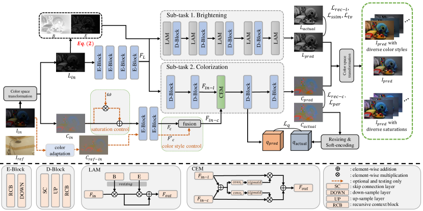
(a)

Figure 2. Framework of the proposed method. The proposed method adopts multi-task learning architecture, containing one encoder and two task-specific decoders. It implements two sub-tasks: brightening and colorization. After model training is completed, the input chrominance can be manipulated by users to achieve enhancement with diver styles and saturations.

2. Related Work

2.1. Low-Light Image Enhancement

Traditional low-light image enhancement (LLIE) methods can be broadly categorized into two types: Histogram Equalization (HE)-based methods (Pizer et al., 1987) and Retinex-based methods (Jobson et al., 1997; Rahman et al., 2004). HE-based methods aim to flatten the histograms of low-light images, while Retinex-based methods attempt to decompose low-light images into illumination and reflectance components. However, these traditional methods often struggle with noise and color. In recent years, Deep Neural Networks (DNNs) have shown great potential for image enhancement (Lore et al., 2017; Zhang et al., 2022; Huang et al., 2022; Li et al., 2023; Kim et al., 2021; Jin et al., 2020, 2019; Kim et al., 2020a; Wu et al., 2022). The first Convolutional Neural Network (CNN) architecture designed for LLIE was proposed by Lore et al. (Lore et al., 2017), and since then, several other CNN-based architectures (Gharbi et al., 2017; Kim et al., 2021, 2020a; Wu et al., 2022) have been proposed. To achieve more realistic results, Retinex theory has been incorporated into DNNs (Wei et al., 2018; Zhang et al., 2019, 2021b; Yang et al., 2021). Methods in (Guo et al., 2020; Wang et al., 2019; Zhang et al., 2022) apply an additional constraint on color information. Besides, many unsupervised methods (Jiang et al., 2021; Guo et al., 2020; Liu et al., 2021; Ma et al., 2022) have been proposed to eliminate the requirement of paired training data. However, these methods often do not make optimal use of chrominance.

Another line of LLIE methods aims to achieve customized enhancement to satisfy the different preferences of users. The first method to introduce customization to LLIE was PieNet (Kim et al., 2020b), which achieved customized enhancement by extracting style vectors from reference images. TSFlow (Wang et al., 2022) introduced style vectors to normalizing flow (Kingma and Dhariwal, 2018) to obtain diverse results. However, these ”black-box” processes may lead to poor flexibility for user customization. ReLLIE (Zhang et al., 2021a) achieved enhancements with different brightness by introducing deep reinforcement learning, but it ignores chrominance information. iUP-Enhancer (Zheng et al., 2022) provided a ”white-box” approach to accomplish customized enhancement by leveraging histogram information in the HSV color space. While histograms as a form of global information may hardly ensure local consistency. Compared to existing customized LLIE methods, BCNet provides a new perspective by using image colorization to achieve customization. This approach preserves lightness details well and allows for accurate chrominance.

2.2. Image Colorization

Image colorization techniques can be classified into two categories: automatic colorization and user-guided colorization. Automatic colorization (Zhang et al., 2016; Guadarrama et al., 2017; Kumar et al., 2020) aims to colorize grayscale images without any external color guidance. Zhang et al. (Zhang et al., 2016) transformed image colorization into a classification task to generate diverse colorization results. Kumar et al. (Kumar et al., 2020) introduced transformer (Vaswani et al., 2017) to image colorization. However, automatic colorization methods often suffer from color ambiguity. To address this issue, user-guided image colorization methods were proposed. Zhang et al. (Zhang et al., 2017) utilized color strokes as color guidance, while He et al. (He et al., 2018), Lu et al. (Lu et al., 2020), and Yin et al. (Yin et al., 2021) used exemplar images as color references. Moreover, to achieve more precise colorization, some methods (Su et al., 2020; Zhao et al., 2020) incorporated semantic information to provide object boundaries and object-specific colorization. In this work, we present a user-guided colorization method that leverages the chrominance information of low-light images to provide not only color guidance but also object boundary information. We also introduce the concept of color classification (Zhang et al., 2016) and apply both regression and classification constraints to achieve more robust colorization.

3. Method

3.1. “Brighten-and-Colorize”

To accomplish the “brighten-and-colorize” enhancement, we first decompose the image into lightness and chrominance. In widely used RGB color space, every single channel contains part of lightness and chrominance, which means they are inseparable in the RGB color space. Therefore, to separate lightness and chrominance, we transform the image from RGB color space to CIELAB color space, where the “L” channel represents lightness and the “AB” channels represent chrominance. Note that we follow the commonly used color space transform function in the image colorization field.

After decomposing the image, the LLIE task is decoupled into two sub-tasks: brightening and colorization. The brightening itself can be regarded as an LLIE problem that predicts lightness with well exposure and details. The colorization aims to predict realistic and accurate chrominance based on the normal-light lightness information and low-light chrominance like user-guide image colorization methods.

3.2. Network Architecture

In this sub-section, we present the details of the proposed method BCNet shown in Fig. 2. BCNet adopts multi-task learning architecture and contains an encoder and two task-specific decoders. Given a low-light image $I_{in}\in\mathbb{R}^{H\times W\times 3}$, we first decompose it into a lightness map $L_{in}\in\mathbb{R}^{H\times W\times 1}$ and a chrominance map $C_{in}\in\mathbb{R}^{H\times W\times 2}$. Then, the encoder takes $L_{in}$ as input and two task-specific decoders output a predicted lightness $L_{pred}\in\mathbb{R}^{H\times W\times 1}$ and a predicted chrominance $C_{pred}\in\mathbb{R}^{H\times W\times 2}$, respectively. The constraints are applied with lightness of ground-truth $L_{actual}\in\mathbb{R}^{H\times W\times 1}$ and chrominance of ground-truth $C_{actual}\in\mathbb{R}^{H\times W\times 2}$. In the following parts, we illustrate the reasonability for adopting the multi-task learning design and the details of two task-specific decoders.

3.2.1. Multi-Task Encoder

The structure content of the lightness is essential for the brightening and colorization sub-tasks. It determines the network how to brighten and where to colorize. In this work, the brightening sub-task aims to recover the clear structure content of lightness, and the colorization sub-task predicts the lost chrominance based on the clear structure content. Due to different inputs, the two sub-tasks are not in the typical design of multi-task learning. However, when training the brightening sub-task, the encoder can learn the information of the clear structure content, which is necessary for the colorization sub-task. By sharing the same encoder, this necessary information for the colorization sub-task can be obtained from the brightening sub-task. Hence, it still can be regarded as a multi-task learning problem. Further, this design not only encourages the information interactions between two sub-tasks but also makes the network more efficient.

Referring to Fig. 2, the multi-task encoder takes the low-light lightness image as input and contains four encoding blocks (E-Block). Every encoding block consists of a Recursive Context Block (RCB) (Zamir et al., 2022), which provides a more effective feature extraction, and a down-sample layer. In this way, we can extract the features $F_{L}$ from $L_{in}$ as:

(1) $$F_{L}=Encoder(L_{in})$$

Note that the output of every encoding block is transmitted to the corresponding decoding block in two sub-tasks by skip-connection layers.

3.2.2. Lightness Decoder

The lightness decoder is adopted in the brightening sub-task. It contains four decoding blocks (D-Block) and five Lightness Adjustment Modules (LAMs). Every decoding block consists of a skip-connection layer, an up-sample layer, and an RCB. The LAM is proposed for guiding the network to improve contrast and preserve better details. Empirically, the darker regions of a low-light image need to be brightened more than brighter regions, and the edges information is essential for an enhanced image. Hence, LAM first takes the inverted map $B$ of $L_{in}$ as the attention prior to indicate where needs more contrast improvement. Then, it utilizes the edge map $E$ of $L_{in}$ to help preserve edges. As shown in Fig. 2, the LAM can be formulated as:

(2) $$B=1-L_{in},E=edge(L_{in})$$

(3) $$F_{out}=F_{in}\times\psi(B)\times(1+\psi(E))$$

where $F_{in}$ and $F_{out}$ are input and output features, respectively. $\psi(.)$ represents resizing operation (bilinear is adopted in this work). $edge$ denotes an edge extractor, which is a $sobel$ operator with kernel size of 3. Then, the predicted lightness $L_{pred}$ can be obtained by:

(4) $$L_{pred}=Brightening(F_{L},B,E)$$

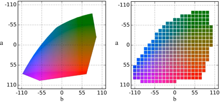
Figure 3. The quantization operation (Zhang et al., 2016) in CIELAB color space. The continuous colors (left) are quantized to 313 discrete colors (right) with a grid size of 10.

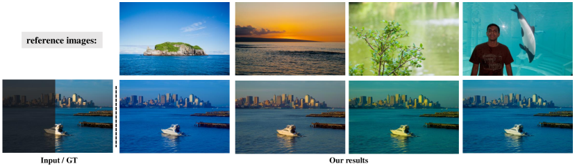
Figure 4. The visual results of color style control. It can be seen that the enhanced results have different color styles based on different reference images.

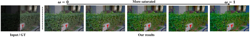
Figure 5. The visual results of saturation control. It can be seen that the result becomes more saturated as the value of $\omega$ goes up.

3.2.3. Chrominance Decoder

The chrominance decoder is adopted in the colorization sub-task, which contains four decoding blocks and a Color Embedding Module (CEM).

Colorization by the low-light chrominance. As mentioned before, colorization is an ill-posed problem, since the color of a certain object is ambiguous. Existing image colorization methods address this issue through the user-guide strategy that introduces an exemplar image or color strokes as color hints. The exemplar image can offer a specific color style, and the color strokes provide approximate guidance. Besides, the colorization methods easily colorize one object beyond its boundary, and this problem can be relieved by introducing semantic information, which reflects the boundaries of objects, to the colorization process. However, different from the original image colorization tasks, in this work, the low-light images already contain part of the chrominance information. Although it is unsaturated, it can provide enough clues to help generate the proper chrominance. For example, the chrominance $C_{in}$ in Fig. 2 is from the input low-light image, it still reflects the approximate color tone and shapes of the ground-truth chrominance $C_{actual}$.

Therefore, we utilize this information by embedding the features of $C_{in}$ to the chrominance decoder. Inspired by (Li et al., 2019), we regard features extracted from lightness and chrominance as multi-scale (i.e., multiple information sources) features and propose a CEM to accomplish feature fusion. As shown in Fig. 2, given the input features $F_{in-l}$ extracted from $L_{in}$ and $F_{in-c}$ extracted from $C_{in}$, CEM first get the summation feature $\hat{F_{in}}$ of two features by element-wise addition as:

(5) $$\hat{F_{in}}=F_{in-l}+F_{in-c}$$

Then, we calculate affinity matrices $A_{l},A_{c}$, which are used to embed chrominance features to the colorization process, by two convolutional layers and $sigmoid$ activations as:

(6) $$A_{l}=sigmoid(conv_{l}(\hat{F_{in}})),A_{c}=sigmoid(conv_{c}(\hat{F_{in}}))$$

Finally, the output feature $F_{out}$ of CEM is obtain by:

(7) $$F_{out}=F_{in-l}\times A_{l}+F_{in-c}\times A_{c}$$

Colorization free from color vanishment. Regarding colorization as a regression task easily results in color vanishment. For example, the day sky is blue and the dusk sky is red, while the mean of red and blue is gray. To relieve this problem, we quantize entire colors in CIELAB color space to 313 categories with a grid size of 10 (as shown in Fig. 3) and calculate the classification loss followed by (Zhang et al., 2016). It is an effective solution for color vanishment. Note that the classification output $q_{pred}\in\mathbb{R}^{h\times w\times 313}$ hardly reaches the original size of the image limited by memory. We set $h$ and $w$ to a quarter of the original size. However, it may affect the enhanced result at the pixel-level. On the other hand, the quantized operation can also lead to performance degradation. Therefore, we apply constraints on color classification output and chrominance map simultaneously, which is helpful for generating various colors and more precise colors at pixel-level, respectively. The predicted chrominance map $C_{pred}$ and color classification output $q_{pred}$ can be expressed by:

(8) $$C_{pred},q_{pred}=Colorization(F_{L},C_{in})$$

3.3. Loss Functions

We apply different constraints in the brightening and colorization sub-tasks based on their different characteristics. For lightness losses, Charbonnier loss (Lai et al., 2018) is first applied as the reconstruct loss $\mathcal{L}_{rec-l}$ to supervise lightness reconstruction at pixel-level, which can be defined as:

(9) $$\mathcal{L}_{rec-l}=\sqrt{\left\|L_{actual}-L_{pred}\right\|_{2}+\epsilon^{2}}$$

where $\epsilon$ is set to $10^{-3}$ empirically. Then, the SSIM (Wang et al., 2004) loss $\mathcal{L}_{ssim}$ and total variation (Chambolle, 2004) loss $\mathcal{L}_{tv}$ are applied to get a better structural details. For chrominance losses, as analyzed in (Zhang et al., 2017, 2016), L2 loss is not robust for colorization due to the inherent multi-modal nature of colorization. In this work, we apply L1 loss as chrominance reconstruction loss $\mathcal{L}_{rec-c}$, which is described as:

(10) $$\mathcal{L}_{rec-c}=\left\|C_{actual}-C_{pred}\right\|_{1}$$

Next, the perceptual loss $\mathcal{L}_{per}$, which constrains in features extracted from VGGNet(Simonyan and Zisserman, 2014), is adopted to get better visual results.

Then, color classification loss $\mathcal{L}_{q}$ is applied to get various colors. The $\mathcal{L}_{q}$ is defined as:

(11) $$\mathcal{L}_{q}=\mathcal{H}(q_{actual},q_{pred})$$

where $\mathcal{H}(.)$ is a 2-D cross-entropy loss function. $q_{actual}$ is obtained by soft-encoding resized $C_{actual}$ as (Zhang et al., 2016).

The total loss of BCNet $\mathcal{L}_{total}$ can be formulated as:

(12) $$\begin{split}\mathcal{L}_{total}=&\lambda_{1}\mathcal{L}_{rec-l}+\lambda_{2}\mathcal{L}_{ssim}+\lambda_{3}\mathcal{L}_{tv}+\\ &\lambda_{4}\mathcal{L}_{rec-c}+\lambda_{5}\mathcal{L}_{per}+\lambda_{6}\mathcal{L}_{q}\end{split}$$

where $\lambda_{1},\lambda_{2},\lambda_{3},\lambda_{4},\lambda_{5},\lambda_{6}$ are weigh factors and set to 1, 0.1, 0.01, 1, 0.01, 0.01, respectively.

3.4. Customized Enhancement

The chrominance of low-light images is served as color guidance to help the colorization sub-task. It provides two essential pieces of information: 1) boundaries information for guiding where to colorize, and 2) color hints for guiding what color to be used. When model training is completed, users can modify the color guidance to achieve customized enhancement. This process only needs to maintain the boundaries information of color guidance to ensure the position of predicted chrominance. Meanwhile, the lightness component is lossless after customized operations since the guidance only affects the colorization sub-task. In this work, two customized operations, which achieve color style control (see Fig. 4) and color saturation control (see Fig. 5), are proposed as follows.

3.4.1. Color Style Control

To generate results with diverse color styles, the color hints provided by guidance can be modified. However, since the boundary information needs to be preserved, manually modifying them may be complicated. One effective solution is to introduce a reference image. There are many color style transfer works (He et al., 2018; Lu et al., 2020; Yin et al., 2021) that can transmit the color style from a reference image to the input image. In our case, since the modification is applied to the guidance, we do not need to explore a complex and accurate transfer. Therefore, we adopt a traditional non-learning color transfer method (Reinhard et al., 2001), which achieves color transfer by transforming images to an orthogonal color space (the detailed implementation can be found in supplementary materials), to obtain customized color guidance (as shown in Fig. 6 (c)). However, this traditional method may hardly perform well in some color details when the input and reference images are irrelevant (as shown in Fig. 6 (d)). To address this issue, we fuse the features $F_{c}$ extracted from $C_{in}$ into the features $F^{\prime}_{c}$ extracted from $C_{ref-in}$ to retain the color details (as shown in Fig. 6 (e)). The fusion process is defined as $(1-\gamma)\times F_{c}+\gamma\times F^{\prime}_{c}$, where $\gamma$ is a hyper-parameter that balances the two features and is set to 0.7 for testing and 0 for training.

3.4.2. Saturation Control

The color guidance provides what color should be used, besides, its intensity also can affect the saturation of output. To preserve the boundaries information, a simple amplified operation is designed as shown in “saturation control” of Fig. 2. The amplified color guidance is obtained by $C_{in}\times(1+\omega)$, where $\omega$ is a hyper-parameter to control the saturation. The bigger $\omega$ represents the result is more saturated and colorful (see Fig. 5). Actually, $\omega$ can be any value, we empirically set $\omega\in[0,1]$. When $\omega<0$ or $\omega>1$, the results may be over dull or saturated.

Note that the above customized operations are not involved in model training. They are optional and only run in the testing phase.

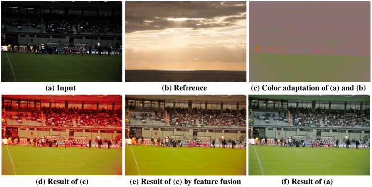
Figure 6. The process of color style control. The input image (a) and reference image (b) first through a color adaptation module (Reinhard et al., 2001) to get customized color guidance (c). (d) is the result of directly embedding (c) to the colorization process, (e) is the result of embedding (c) to the colorization process with a feature fusion module, and (f) is the result of directly embedding the original chrominance of (a) to the colorization process. By comparing (d), (e), and (f), we can find the color style of (b) is transferred to (e) and the feature fusion module is helpful for keeping the color details.

4. Experiment

Table 1. Quantitative comparison on the LOL-real (Yang et al., 2021) and FiveK (Bychkovsky et al., 2011). The best results are boldfaced and the second-best ones are underlined.

Methods	LOL-real (Yang et al., 2021)					FiveK (Bychkovsky et al., 2011)					Size (M)
	PSNR $\uparrow$	SSIM $\uparrow$	$\Delta E\_{ab}$$\downarrow$	LPIPS $\downarrow$	CSE (ratio) $\downarrow$	PSNR $\uparrow$	SSIM $\uparrow$	$\Delta E\_{ab}$ $\downarrow$	LPIPS $\downarrow$	CSE (ratio) $\downarrow$
DRD(Wei et al., 2018)	16.08	0.6555	22.35	0.2364	2.53	21.68	0.8604	10.52	0.0574	2.18	0.86
Kind(Zhang et al., 2019)	20.01	0.8412	12.53	0.0813	1.30	20.71	0.8835	10.75	0.0480	1.38	8.02
Kind++(Zhang et al., 2021b)	20.59	0.8294	12.51	0.0875	1.18	19.71	0.8640	14.05	0.0574	2.12	8.27
MIRNet(Zamir et al., 2020)	22.11	0.7942	10.11	0.1448	1.35	24.41	0.9097	7.90	0.0344	1.33	31.79
EnGAN(Jiang et al., 2021)	18.64	0.6767	17.73	0.1512	6.18	15.38	0.7752	18.89	0.0984	2.97	8.64
DeepUPE(Wang et al., 2019)	18.68	0.5791	17.54	0.1868	9.48	24.24	0.8957	8.16	0.0440	2.15	0.99
DeepLPF(Moran et al., 2020)	20.03	0.7819	12.58	0.1460	3.23	24.74	0.9170	7.50	0.0570	1.44	1.72
UEGAN(Ni et al., 2020)	20.30	0.7417	14.69	0.1464	12.97	23.00	0.8717	9.96	0.0503	3.84	4.16
SGM(Yang et al., 2021)	20.06	0.8158	11.36	0.0727	1.33	22.57	0.8823	9.36	0.0557	4.23	2.31
MIRNet-v2(Zamir et al., 2022)	21.83	0.8455	11.47	0.0666	1.49	25.04	0.9188	8.05	0.0357	1.54	5.86
SNR-Aware(Xu et al., 2022)	21.48	0.8478	10.58	0.0740	1.14	25.41	0.9234	7.24	0.0293	1.49	39.12
Ours	23.27	0.8637	8.97	0.0566	1.00	25.74	0.9285	6.77	0.0291	1.00	6.84

4.1. Datasets and Implementation Details

LOL-real (Yang et al., 2021) and MIT-Adobe-FiveK (Bychkovsky et al., 2011) (for short called FiveK) are adopted as our experimental datasets. LOL-real is captured in the real world by changing exposure time and ISO. It contains 689 pairs of low-/normal-light images for training and 100 pairs for testing. FiveK contains 5,000 raw images and corresponding five high-quality versions retouched by experts. The version retouched by expert C is adopted as the ground-truth and it is divided into 4,500 training pairs and 500 testing pairs following (Wang et al., 2019; Zamir et al., 2022).

BCNet is implemented in PyTorch and trained in an RTX2080Ti GPU with batch size of 8. The learning rate is initiated to $2.0\times 10^{-4}$ and a multi-step scheduler is adopted. Adam (Kingma and Ba, 2015) with momentum of 0.9 is adopted as the optimizer. Input training images are randomly cropped to $256\times 256$ and rotated by multiples of 90 degrees.

4.2. Comparison with Recent LLIE Methods

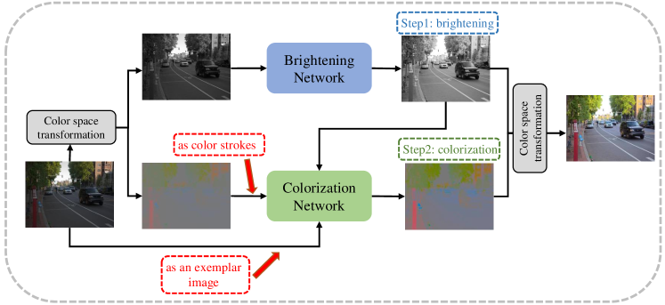
Figure 7. The illustration of the two-step “brighten-and-colorize”. Note that the exemplar-based colorizer takes the low-light image as color hints and the stroke-based colorizer takes the chrominance of the low-light image as color hints.

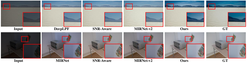
Figure 8. The qualitative comparison on FiveK (Bychkovsky et al., 2011) (the first row) and LOL-real (Yang et al., 2021) (the second row). It can be seen that the proposed method reaches the best visual results.

We compare BCNet with recent SOTA LLIE methods, which include DRD (Wei et al., 2018), Kind (Zhang et al., 2019), Kind++ (Zhang et al., 2021b), MIRNet (Zamir et al., 2020), EnGAN (Jiang et al., 2021), DeepUPE (Wang et al., 2019), DeepLPF (Moran et al., 2020), UEGAN (Ni et al., 2020), SGM (Yang et al., 2021), MIRNet-v2 (Zamir et al., 2022), and SNR-Aware (Xu et al., 2022). Note that we load the pre-trained parameters of EnGAN and retrain other methods on the same datasets.

Quantitative comparison. In this work, PSNR, SSIM (Wang et al., 2004), the $L_{2}-distance$ in CIELAB color space ($\bigtriangleup E_{ab}$), LPIPS (Zhang et al., 2018), and Color-Sensitive Error (CSE) (Zhao et al., 2021) are employed as the evaluation matrices. Note that LPIPS measures the distance of high-level features between two images, and CSE measures the color difference between two images. We employ the ratio of our result as the unit of CSE following recent works (Zhang et al., 2022; Zhao et al., 2022). In general, the lower LPIPS, lower CSE, lower $\bigtriangleup E_{ab}$, higher SSIM, and higher PSNR values represent two images with more relative low-/high- level features. Table 1 shows the quantitative comparisons of LOL-real and FiveK. The proposed method achieves the best results on all metrics benefiting from the decoupled strategy. It demonstrates that enhanced images of our method are closer to ground-truth no matter in structure, color, or high-level features. Besides, we also present the comparison of model size. As shown in Table 1, the size of the proposed method is comparable to other methods.

Qualitative comparison. We present the visual results of two datasets in Fig. 8 for comparing the proposed method with some baselines good at PSNR. It can be seen that although existing methods reach decent lightness, they are hard to recover chrominance well (e.g., the color of the sky in Fig. 8). While the proposed method can obtain satisfying results. Besides, the proposed method achieves customized enhancement as shown in Fig. 4 and Fig. 5. The users can enhance low-light images as per their preferences.

4.3. Comparison with Two-Step “Brighten-and-Colorize” Methods

We also compare BCNet with other two-step “brighten-and-colorize” methods, which are composed of a brightener (brightening network) and a colorizer (colorization network). The brightener is an LLIE method, whose input and output are single-channel lightness. The colorizer is a user-guide image colorization method, which takes the low-light image as color hints and predicts chrominance based on the output of brightener and color hints. The implementation details of the two-step “brighten-and-colorize” can refer to Fig. 7. For brighteners, we choose SNR-Aware (Xu et al., 2022) and MIRNet-v2(Zamir et al., 2022). For colorizers, we choose an exemplar-based Yin et al. (Yin et al., 2021) method and a stroke-based Zhang et al. (Zhang et al., 2017) method. Then, we pair them up to get four methods. Note that the brighteners need to be retrained on our datasets since the mismatched input/output channels of networks. The stroke-based colorizer is easy to be retrained as well. While for the exemplar-based colorizer, it is hard to be retrained in traditional LLIE datasets, since it needs to calculate similarities between the input image and the exemplar image, and query color from the database when lacking matched colors in the exemplar image. Therefore, we opt to solely retrain the stroke-based colorizer,

while utilizing the pre-trained exemplar-based colorizer.

The quantitative comparison is presented in Table 2. We adopt PSNR, SSIM, and CSE as the assessment metrics, and it can be seen that the proposed method obtains the best performance. Fig. 9 shows the qualitative results. For the exemplar-based colorizer, which aims to transfer color from the exemplar image to the input lightness, the generated color is unsaturated due to the unsaturated exemplar image (i.e., input low-light image). On the other hand, color hints in stroke-based colorization are just provided as approximate guidance. Although the input color is unsaturated, the generated color of the stroke-based colorizer is bright. After retraining, the generated color can be more realistic. For example, the input color of the Ping-Pong table in Fig. 9 is dull blue, therefore, the result of exemplar-based colorizer is still dull blue, while stroke-based colorizer can generate bright blue and retrained stroke-based colorizer can generate more realistic bright blue. However, the result of the proposed method is more accurate and saturated.

4.4. Analysis

Table 2. Quantitative comparison with two-step “brighten-and-colorize” methods on LOL-real (Yang et al., 2021) dataset. The best results are boldfaced and the second-best ones are underlined. Note that “*” represents this method is retrained.

Brightener	Colorizer	PSNR $\uparrow$	SSIM $\uparrow$	CSE(ratio) $\downarrow$
SNR-Aware (Xu et al., 2022)	Zhang et al.* (Zhang et al., 2017)	20.90	0.8304	1.34
	Zhang et al. (Zhang et al., 2017)	11.81	0.5411	70.44
	Yin et al. (Yin et al., 2021)	19.69	0.7881	7.40
MIRNet-v2 (Zamir et al., 2022)	Zhang et al.* (Zhang et al., 2017)	21.91	0.8242	1.09
	Zhang et al. (Zhang et al., 2017)	12.01	0.5313	77.60
	Yin et al. (Yin et al., 2021)	20.44	0.7810	7.30
Ours		23.27	0.8637	1.00

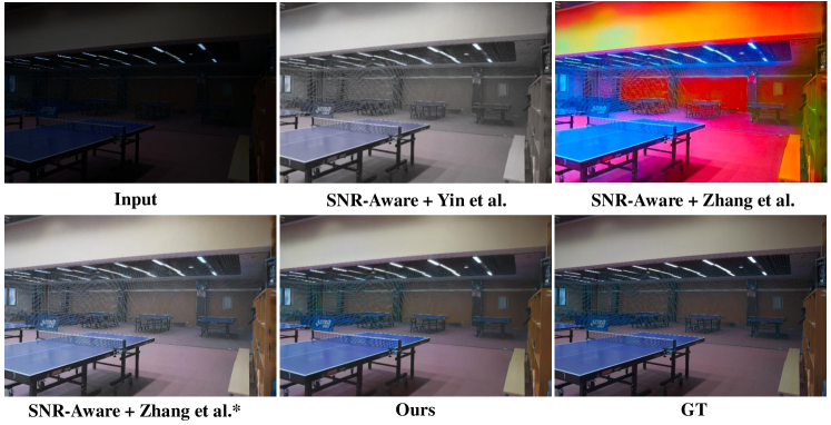
(a)

Figure 9. The qualitative comparison with “brighten-and-colorize” methods. Note that two brighteners have similar visual results, we only present the results of SNR-Aware (Xu et al., 2022).

Ablation study. We conduct the ablation study on five different settings to demonstrate the effectiveness of the proposed designs: (1) “W/o Decoupling” adopts an encoder-decoder architecture and predicts enhanced results in RGB color space; (2) “W/o Sharing” adopts two-step “brighten-and-colorize”, where brightener and colorizer are based on the proposed designs; (3) “W/o LAM” removes the lightness adjustment module; (4) “W/o CEM” removes the color embedding module and adopts concatenation; (5) “W/o $\mathcal{L}_{q}$” removes color classification loss.

We report the ablation study results in Table 3. We can see that our full setting yields the best PSNR, SSIM, and second-best CSE. “W/o Decoupling” verifies the effectiveness of this decoupled enhancement mode. “W/o $\mathcal{L}_{q}$”, “W/o Sharing”, “W/o LAM”, and “W/o CEM” verify the effectiveness of the proposed corresponding designs. Fig. 10 presents the visual results of ablation studies. “W/o $\mathcal{L}_{q}$”, “W/o Sharing”, and “W/o CEM” hardly perform well in chrominance. “W/o LAM” may lead to worse performance in lightness. “W/o Decoupling” suffers from both above problems. Our result reaches the best visual quality. It is worth mentioning that although the quantitative results of “W/o $\mathcal{L}_{q}$” have only a few reductions, the qualitative result suffers from a little color vanishment (e.g., the color of grasses). It verifies the effectiveness of $\mathcal{L}_{q}$. Besides, we also conduct the ablation study in the other loss functions and adopted color spaces, which can be found in the supplementary materials.

Table 3. Ablation studies on LOL-real (Yang et al., 2021) dataset. The best results are boldfaced and the second-best ones are underlined.

Methods	PSNR $\uparrow$	SSIM $\uparrow$	CSE(ratio) $\downarrow$	Size (M)
W/o Decoupling	21.28	0.8003	3.05	4.22
W/o Sharing	23.03	0.8591	1.12	8.44
W/o LAM	22.77	0.8516	0.91	6.84
W/o CEM	23.06	0.8575	1.66	6.84
W/o $\mathcal{L}_{q}$	23.21	0.8600	1.11	6.84
Ours	23.27	0.8637	1.00	6.84

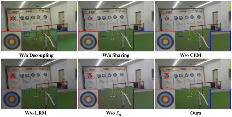
(a)

Figure 10. The qualitative comparison of ablation studies.

Limitation. The precondition of the colorization sub-task is that the chrominance of the input image contains a little color tone and shapes. However, when the input image is extremely dark, it hardly provides enough information for colorization. As a result, the chrominance of the enhanced image is very dull as shown in Fig. 11. Actually, it may be relieved by the automatic colorization methods, which is also one of our future works.

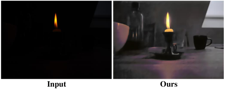
(a)

Figure 11. Failure case. When the input image is extremely dark, we hardly predict proper chrominance, since the input image hardly provides enough chrominance information.

5. Conclusion

In this work, we novelly introduce image colorization to LLIE and propose a “brighten-and-colorize” enhancement network BCNet for low-light images. Based on the relation of image colorization and LLIE, we treat this enhancement as a multi-task learning problem. A low-light image is decomposed to lightness and chrominance and fulfills the decoupled enhancement by the proposed BCNet. BCNet contains a multi-task encoder and two task-specific decoders, which are designed elaborately according to different characteristics of lightness and chrominance. Based on the decoupled design, BCNet further achieves lightness-invariant customization with diverse saturations and color styles by manipulating the color guidance of the colorization sub-task. Extensive experiments demonstrate that BCNet sets the current SOTA results in LLIE and flexible customization. In the future, we will explore more effective ways to introduce image colorization to other image restoration tasks.

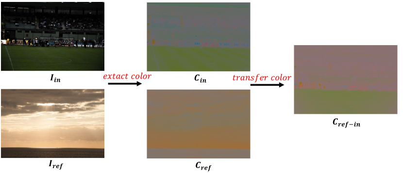
Figure 12. The process of color adaptation.

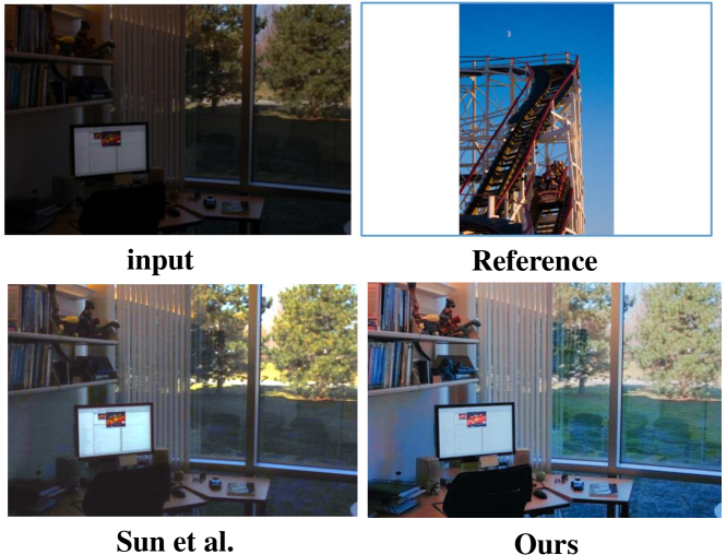
Figure 13. Visual comparison with other Su et al. (Sun et al., 2021).

Appendix A Additional Ablation Studies

Loss functions. We further conduct an ablation study on loss functions.

• “W/o $\mathcal{L}_{ssim}$” removes ssim loss in brightening sub-task.

• “W/o $\mathcal{L}_{tv}$” removes smooth loss in brightening sub-task.

• “W/o $\mathcal{L}_{per}$” removes perceptual loss in colorization sub-task.

The results in Table 4 demonstrate the effectiveness of adopted loss functions.

Color spaces. In fact, there are several color spaces that can decompose an image into lightness and chrominance, such as HSV, HSI, Luv, Yuv, et al.. We conduct an ablation study on color spaces to verify the effectiveness of adopted Lab color space. However, since it is hard to quantize chrominance channels in other color spaces like (Zhang et al., 2016) in Lab color space, we present the results of removing color classification loss in Lab color space for a fair comparison. As shown in Table 6, the Lab achieves the best results. Actually, it is also the popular color space in the image colorization field.

Table 4. Results of the loss functions ablation studies on LOL-real (Yang et al., 2021) dataset. The best results are boldfaced and the second-best ones are underlined.

Methods	PSNR	SSIM	LPIPS	CSE (ratio)
w/o $\mathcal{L}_{ssim}$	22.40	0.8388	0.0801	1.01
w/o $\mathcal{L}_{tv}$	22.02	0.8454	0.0739	1.39
w/o $\mathcal{L}_{per}$	22.92	0.8582	0.0729	1.99
Ours	23.27	0.8637	0.0566	1.00

Table 5. Quantitative comparison with customized LLIE methods.

Methods	PieNet (Kim et al., 2020b)	Sun te al. (Sun et al., 2021)	TSFlow (Wang et al., 2022)	Ours
PSNR(dB)	25.28	20.87	25.57	25.74

Table 6. Results of the color space ablation studies on LOL-real (Yang et al., 2021) dataset. The best results are boldfaced and the second-best ones are underlined.

Methods	PSNR	SSIM	LPIPS	CSE (ratio)
HSV	22.02	0.8257	0.0809	1.12
HLS	22.31	0.8454	0.0869	1.38
Luv	22.02	0.8420	0.0702	1.06
Yuv	22.37	0.8416	0.0751	1.16
Lab (ours)	23.21	0.8600	0.0619	1.00

Appendix B Comparison with other customized LLIE method

We conduct the comparison with other customized LLIE methods in Table. 5 and Fig. 13. Note that we only compare the visual result with Sun et al. (Sun et al., 2021) since only their method is based on one reference image and opens the source code. As can be seen, the proposed method reaches accurate and flexible enhancement.

Appendix C Implementation of Color Adaptation

The color adaptation is responsible for generating customized color guidance based on a reference image. We utilize a non-learning method (Reinhard et al., 2001) to accomplish this process. Given an input low-light image $I_{in}$ and a reference image $I_{ref}$, we first transform them into CIELAB color space:

(13) $$\begin{split}L_{in},a_{in},b_{in}=RGB2Lab(I_{in})\\ L_{ref},a_{ref},b_{ref}=RGB2Lab(I_{ref})\\ \end{split}$$

where $RGB2Lab(.)$ represents the color space transform function. Then, the mean value and standard deviation are used to transfer color:

(14) $$\begin{split}a_{in}=a_{in}-mean(a_{in}),b_{in}=b_{in}-mean(b_{in})\\ \end{split}$$

(15) $$\begin{split}a_{in}=a_{in}\times(std(a_{in})/std(a_{ref}))\\ b_{in}=b_{in}\times(std(b_{in})/std(b_{ref})\\ \end{split}$$

where $mean(.)$ and $std(.)$ represent to extract the mean value and standard deviation. Finally, the transferred color guidance $C_{ref-in}=cat(a_{in},b_{in})$. The visual result can be seen in Fig. 12. Note that the focus of color adaptation is the chrominance information, we ignore the lightness components of two images.

Appendix D More Visual results

We present more customized enhancement results in Fig. 14 (enhancement with diverse saturations) and Fig. 15 (enhancement with diverse color styles).

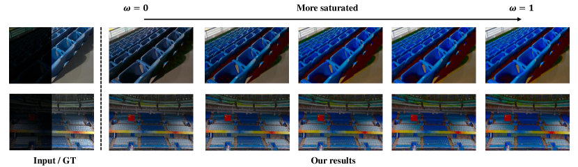
(a)

Figure 14. Enhancement with diverse saturations.

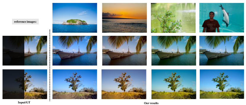
(a)

Figure 15. Enhancement with diverse color styles.