Lorentz Invariance Violation Limits from GRB 221009A

Abstract

It has been long conjectured that a signature of Quantum Gravity will be Lorentz Invariance Violation (LIV) that could be observed at energies much lower than the Planck scale. One possible signature of LIV is an energy-dependent speed of photons. This can be tested with a distant transient source of very high-energy photons. We explore time-of-flight limits on LIV derived from LHAASO’s observations of tens of thousands of TeV photons from GRB 221009A, the brightest gamma-ray burst of all time. For a linear ($n=1$) dependence of the photon velocity on energy, we find a lower limit on the LIV scale of ${5.9}(6.2)\ E_{\rm pl}$ for subluminal (superluminal) modes. These are comparable to the stringent limits obtained so far. For a quadratic model ($n=2$), the limits, which are currently the best available, are much lower, $5.8(4.6)\times 10^{-8}\ E_{\rm pl}$. Our analysis uses the publicly available LHAASO data which is only in the $0.2-7$ TeV range. Higher energy data would enable us to improve these limits by a factor of 3 for $n=1$ and by an order of magnitude for $n=2$.

I Introduction

The Gamma-Ray Burst (GRB) 221009A was an extremely powerful nearby ($z=0.151$) burst, the brightest ever detected. Among its numerous unique features was the detection of tens of thousands of TeV ($0.2-18\,$TeV) photons [1]. The large number of photons enabled the LHAASO collaboration to obtain detailed TeV lightcurve and spectra. The TeV lightcurve, which was very different from the lower energy gamma-rays lightcurve detected by Fermi [2], HXMT [3] and other detectors, confirmed earlier suggestions that the dominant GRBs’ very high energy emission is an afterglow [4, 5, 6, 7, 8, 9] and that the prompt very high energy emission is much weaker.

This TeV lightcurve and spectra enable us to explore the possibility of Lorentz Invariance Violation (LIV) and set limits on the scale in which this may happen. LIV was introduced as a potential low-energy signature of Quantum Gravity-induced corrections to general relativity. Historically, the concept was suggested as a potential explanation for the GZK paradox [10, 11] by introducing a shift in the Delta resonance $p+\gamma\rightarrow\Delta^{+}$ threshold, preventing energy losses of the protons on interaction with the CMB background photons. Later on, it was pointed out that this modification would also introduce a shift in the annihilation threshold of high energy photons by the extragalactic background light (EBL), $\gamma\gamma\rightarrow e^{+}e^{-}$ [12, 13]. When an 18 TeV photon was reported to have arrived from GRB 221009 [14], LIV has been suggested, among several other ‘new physics’ solutions [15]. However, a careful analysis [16, 17] revealed that when errors in estimating the 18 TeV photon’s energy ($\pm 7$ TeV) and the optical depth of the Universe at these energies [18] are taken into account, ‘new physics’ is not essential.

LIV also introduces an energy-dependent photon velocity. This can be tested by comparing the arrival times of different energy photons that have been emitted simultaneously [19]. For this, one needs a distant high-energy transient source with rapid temporal variability. GRBs are the best transients for that. A high fluence distant GRB with a very high energy emission is the best source to explore LIV-induced time-of-flight (TOF) differences: GRB221009A is an ideal source.

We explore here the implication of the rapid rise time of the TeV afterglow to TOF LIV limits. We begin in II with a brief discussion of Quantum Gravity-modified dispersion relations. We describe in III the TeV afterglow data and our LIV limits. We compare in IV our results to earlier LIV limits obtained with GRBs 090510A and 190114C. We conclude, summarizing our findings, in V.

II Lorentz Invariance Violation

A natural expectation for a “low-energy” quantum gravity effect is a modified photon dispersion relation [19]:

$${E^{2}=p^{2}c^{2}\left[1{+\sigma}\left(\frac{E}{{{\cal E}_{\rm QG,n}^{(\sigma)}}E_{\rm pl}}\right)^{n}\right]}\ ,$$ (1)

where $E_{\rm pl}\approx 1.22\times 10^{19}\,$GeV is the Planck energy. ${\cal E}_{\rm QG,n}^{(\sigma)}$ measures the LIV energy scale in units of $E_{\rm pl}$ and the index $\sigma=\pm 1$ denotes the sign of the dispersion modification. Such a dispersion introduces an energy-dependent photon velocity. For $E\ll{\cal E}_{\rm QG,n}E_{\rm pl}$ we have:

$$v=c\left[1+\sigma\frac{n+1}{2}\left(\frac{E}{{\cal E}_{\rm QG,n}^{(\sigma)}E_{\rm pl}}\right)^{n}\right].$$ (2)

Subluminal (superluminal) motion corresponds to $\sigma=-1(+1)$. This leads to an energy-dependent TOF of a photon with energy $E$ as compared to travel at the speed of light [20]:

$$\delta t_{\rm LIV}(E)={-\sigma}\frac{n+1}{2H_{0}}\left(\frac{E}{{\cal E}_{\rm QG,n}^{{(\sigma)}}E_{\rm pl}}\right)^{n}\\ \times\int_{0}^{z}\frac{(1+\zeta)^{n}d\zeta}{\sqrt{\Omega_{\rm m}(1+\zeta)^{3}+\Omega_{\Lambda}}}\ ,$$ (3)

where $z$ is the redshift of the source, $H_{0}=67.5\,$km s${}^{-1}\,$Mpc^-1 is the Hubble-Lemaitre constant, $\Omega_{\rm M}=0.315$ is the current fraction of matter in the Universe, and $\Omega_{\Lambda}=0.685$ the cosmological constant fraction. For GRB 221009A at $z=0.151$ we have:

$$\delta t_{{\rm LIV},z=0.151}(E)={\sigma}\begin{cases}5.7\,\text{s}\,\dfrac{E/{\rm TeV}}{{\cal E}_{\rm QG,1}^{{(\sigma)}}},&{n=1}\\ 7.5\,\text{s}\,\left(\dfrac{E/{\rm TeV}}{10^{8}{\cal E}_{\rm QG,2}^{{(\sigma)}}}\right)^{2},&{n=2}\end{cases}\ .$$ (4)

III LIV limits from GRB 221009A

III.1 GRB 221009A—the brightest burst ever

The extreme brightness of GRB 221009A was due to a combination of an extreme intrinsic luminosity, $E_{\rm iso}\approx 10^{55}$ erg/s and its relatively nearby location $z=0.151$ [21]. It was so bright that it saturated most GRB detectors. However, [DO: data of] Insight-HXMT and GECAM-C [3] were able to detect the exact[DO: , as well as Konus-Wind and ART-XC [Konus-wind], allowed to measure the] prompt lightcurve.

One of the unique features of GRB 221009A, on which we focus here, was LHASSO’s observations of TeV signal [14, 1] with more than 64000 photons in the energy range of $0.2-18$ TeV. The fast-rising and smooth, gradually declining lightcurve of the LHASSO signal [1], which is very different from the prompt lightcurve [3, 2] indicates clearly that the TeV signal was an afterglow (compare Figs. 1 of [3] and 1 of [2] with Fig. 1 of [1]). This interpretation is consistent with earlier suggestions [4, 5, 6, 7] that most of the Fermi-LAT detected GRBs’ GeV emission is an afterglow and that the TeV emission observed from GRB 190114C was from an afterglow [8, 9].

Interestingly, the kinetic energy of the afterglow (both as implied from the TeV emission itself and from the later ($\sim 3000$ s) X-ray afterglow observations [23]) was significantly lower than the one of the prompt emission [3] (and comparable to the one observed in other TeV GRBs [8, 24]). This suggests that the extreme intrinsic properties of the prompt emission probably arose due to an extremely narrow jet [3, 23].

The afterglow lightcurve rises as $t^{1.8}$ from 5 to 14 s (we measure all times relative to the onset of the main prompt emission at ${T_{*}}=226$ s after the Fermi trigger[1]). The spectrum at this stage (see Fig. 2 of [1]) is rather similar to those taken within the intervals $14-22$ s in which the lightcurve is almost flat and $22-100$ in which the lightcurve declines as $t^{-1.115}$ (see Figs. 2 and 3b in [1]). Correspondingly the lightcurves at different energies are similar (see their Figs. 4 and S7).

III.2 LIV limits

Both the highest reported (7 TeV) and the lowest energy (0.2 TeV) photons arrived by 14 s, the end of the first time interval. This puts a limit on the TOF difference between those two photons:

$$\Delta t_{\rm obs}(0.2-{7}~{}{\rm TeV})\leqslant 14(9)\ {\rm s}\ ,$$ (5)

where the limit in bracket takes into account the fact that this interval begins only at 5 s. Comparing the LIV TOF relation, Eq. (4), with the observed limit we obtain $|\delta t_{{\rm LIV,}z=0.151}(0.2-7~{}{\rm TeV})|\leqslant\Delta t_{\rm obs}(0.2-{7}~{}{\rm TeV})$:

$${\cal E}_{\rm QG,1}^{({\pm})} \geqslant{2.8\;(4.3)}, \qquad n =1\ ,$$

$${\cal E}_{\rm QG,2}^{({\pm})} \geqslant{5.1\;(6.4)}\times 10^{-8}, n =2\ ,$$ (6)

where the values in brackets reflect the stronger estimate for $\Delta t_{\rm obs}$. Strictly speaking, these limits could be affected by intrinsic spectral variations. However, as discussed earlier, there were no significant spectral variations during this period, suggesting that intrinsic spectral variations aren’t significant. Thus, Eq. (6) should give correct order-of-magnitude estimate of ${\cal E}_{\rm QG,n}^{(\pm)}$.

We can now refine these limits. In [1] it was shown that the observed spectral flux, [erg^-1 cm^-2 s^-1], for $t=5-100\,$s can be fitted by the form:

$$F(E,t)=A\left(\frac{E}{\rm TeV}\right)^{-\gamma}e^{-E/E_{\rm cut}}\\ \times\left[\left(\frac{t}{t_{\rm b}}\right)^{-\alpha_{1}\omega}+\left(\frac{t}{t_{\rm b}}\right)^{-\alpha_{2}\omega}\right]^{-1/\omega}.$$ (7)

In this time range one can safely consider $\gamma$ and $E_{\rm cut}$ as constants. They, as well as $A$, $t_{\rm b}$, $\alpha_{1,2}$, and $\omega$, could be fitted to the observed lightcurve and spectra of the GRB 221009A afterglow.

To take account of LIV TOF, we modify the flux energy dependence by shifting the arrival of photons according to Eq. (4)

$${F_{\rm LIV}}(E,t;{\cal E}_{\rm QG,n}^{(\sigma)})=F\bigl{(}E,t+\delta t_{LIV,z=0.151}(E,{\cal E}_{\rm QG,n}^{(\sigma)})\bigr{)}.$$ (8)

We fit now this functional form to the LHAASO lightcurve (Fig. 3 of [1]; top panes in Figs. 1 and 2 here) and spectrum during the first three time-bins: $5-14\,$s, $14-22\,$s, and $22-100\,$s (data points from Fig. S4C in [1]; bottom panels in Figs. 1 and 2 here), minimizing the combined $\chi^{2}$. We use as fitting parameters ${\sigma}/{\cal E}_{\rm QG,1}^{{(\sigma)}}$ and ${\sigma}(10^{-8}/{\cal E}_{\rm QG,2}^{{(\sigma)}})^{2}$ whose best-fit values are around zero, rather than ${\cal E}_{\rm QG,1}$ and ${\cal E}_{\rm QG,2}$ whose best-fit values, in case of no LIV, would be infinite. We have assumed that the spectrum hasn’t changed during the time we consider [DO: (]$5-100\,$s[DO: )] and that the data errors are Gaussian. To fit the lightcurve, $\Phi(t)$, we integrate the spectral flux (Eq. 8) over the same energy range as in Fig. 3 of [1], i.e. $0.3-5\,$TeV:

$$\Phi_{\rm LIV}(t,{{\cal E}_{\rm QG,n}^{{(\sigma)}}})=\int_{0.3\,\text{TeV}}^{5\,\text{TeV}}F_{\rm LIV}(E,t;{{\cal E}_{\rm QG,n}^{{(\sigma)}}})E\,\mathrm{d}E.$$ (9)

To fit the spectra, $\psi^{(i)}(E)$ in each time bin $i$, we average the spectral flux over each bin:

$$\psi_{\rm LIV}^{(i)}(E,{{\cal E}_{\rm QG,n}^{{(\sigma)}}})=\frac{C_{\text{a.c.}}}{t_{\text{up}\,i}-t_{\text{low}\,i}}\int_{t_{\text{low}\,i}}^{t_{\text{up}\,i}}F_{\rm LIV}(E,t;{{\cal E}_{\rm QG,n}^{{(\sigma)}}})\,\mathrm{d}t.$$ (10)

Our method to average the spectral flux over the time bins differs from that used by [1]. The latter uses the full data set of LHAASO (energy and arrival time of each photon), which is not available to us. To take the difference into account, we introduce the phenomenological averaging-correction constant $C_{\text{a.c.}}$ using the same $C_{\text{a.c.}}$ for all three time bins. Nevertheless, as shown below, our results are consistent with those of [1].

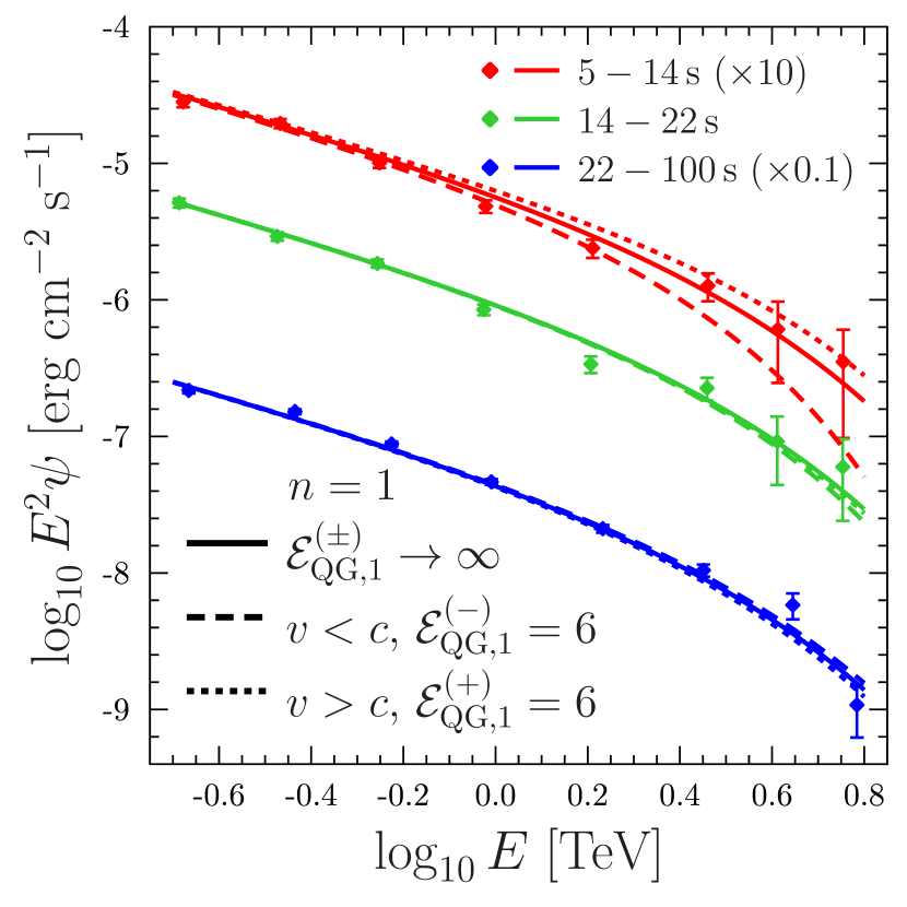
Figure 1: LHAASO data for GRB 221909A [1] and its fitting with linear LIV, $n=1$. Top: the lightcurve $\Phi(t)$ and its fits by Eq. (9). Bottom: spectra $\psi(E)\times E^{2}$ for three time bands and their fits by Eq. (10) The solid, dashed, and dotted lines correspond to ${\cal E}_{\rm QG,1}^{(\pm)}\to\infty$, ${\cal E}_{\rm QG,1}^{(-)}=6$, and ${\cal E}_{\rm QG,1}^{(+)}=6$.

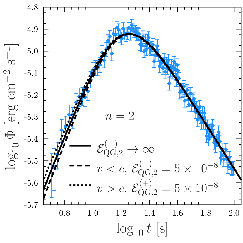
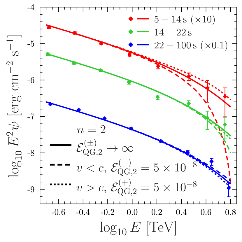
Figure 2: The same as in Fig. 1 but for the quadratic LIV model, $n=2$. The solid, dashed, and dotted lines correspond to ${\cal E}_{\rm QG,1}^{(\pm)}\to\infty$, ${\cal E}_{\rm QG,2}^{(-)}=5\times 10^{-8}$, and ${\cal E}_{\rm QG,2}^{(+)}=5\times 10^{-8}$.

Figs. 1 and 2 illustrate how fitting of the GRB 221009A TeV afterglow constrains the LIV parameters. Solid lines display the best fit with no LIV (${\cal E}_{\rm QG,n}^{{(\pm)}}\to\infty$). Dashed and dotted lines show the results if we turn on sub- and superluminal LIV, respectively, using the same values for all other parameters as for the solid lines. The effect of LIV is two-fold. Subluminal LIV (dashed lines) suppresses the rising phase of the lightcurve and makes the spectrum during this phase ($5-14\,$s) softer. Other effects—intensifying the lightcurve in the fading phase, softening the spectrum at the maximum brightness phase ($14-22\,$s), and hardening the spectrum in the fading phase ($22-100\,$s)—are much less pronounced. For superluminal LIV, all effects but one are inverted (the maximum brightness spectrum is softened in both cases). In both cases, too small ${\cal E}_{\rm QG,n}^{{(\pm)}}$ values give inconsistent discrepancies between the model curves and the data. While for $n=1$, the deviation from the lightcurve dominates, for $n=2$, the deviation from the spectral shape is the most restrictive.

Table 1: Best-fit parameters for the model given by Eq. 8 and a combined $\chi^{2}$ fit for both the lightcurve and the spectra of the afterglow of GRB 221009A in the time region $5-100\,$s. The observational data is taken from [1]. If not specified differently, a fit parameter is dimensionless.

	Best fit	95% confidence interval
$A$	$8.1$	$6.5$ — $9.8$
$C_{\rm a.c.}$	$0.25$	$0.24$ — $0.26$
$t_{\rm b}$	$16.0$	$14.3$ — $17.6$
$\alpha_{1}$	$1.6$	$1.1$ — $2.0$
$\alpha_{2}$	$-1.02$	$-1.08$ — $-0.95$
$\omega$	$1.5$	$0.8$ — $2.1$
$\gamma$	$2.93$	$2.84$ — $3.02$
$E_{\rm cut}$	$3.1$	$2.1$ — $4.1$
${\cal E}_{\rm QG,1}^{{(\sigma)}}$	—	${\cal E}_{\rm QG,1}^{(-)}\geqslant 5.9\ ;{\cal E}_{\rm QG,1}^{(+)}\geqslant 6.2$
${\cal E}_{\rm QG,2}^{{(\sigma)}}$	—	${\cal E}_{\rm QG,2}^{(-)}\geqslant 5.8\times 10^{-8}\ ;\ {\cal E}_{\rm QG,2}^{(+)}\geqslant 4.6\times 10^{-8}$

Results of simultaneous fitting of all nine parameters in Eqs. (7)—(10), eight for the non-violated spectral flux (7) and an additional one for LIV, are presented in Table 1. They are consistent with those calculated in [1] when LIV is not taken into account. The very large best-fit values for both ${\cal E}_{\rm QG,1}^{{(\sigma)}}$ and ${\cal E}_{\rm QG,2}^{{(\sigma)}}$ are consistent with infinity. For ${\cal E}_{\rm QG}^{{(\pm)}}\to\infty$ our results are consistent with those of [1]. The ranges ${\cal E}_{\rm QG,1}^{(-)}<5.9$ and ${\cal E}_{\rm QG,1}^{(+)}<6.2$ and the ranges ${\cal E}_{\rm QG,2}^{(-)}<5.8\times 10^{-8}$ and ${\cal E}_{\rm QG,1}^{(+)}<4.6\times 10^{-8}$ are ruled out at 95% confidence level. Best-fit values and confidence intervals for other parameters are almost the same for both fitting the data with linear LIV, quadratic LIV, and no LIV at all. In all three cases, the minimal $\chi^{2}\approx 164$. Given the number of data points 157 and 9 independent parameters (8 for no LIV), the reduced $\chi^{2}$ values are $1.10-1.11$, signifying a statistically acceptable fit. The limits on ${\cal E}_{\rm QG,1}^{(\pm)}$ we find here are comparable to the strongest limits obtained so far from GRB 090510. The limits on ${\cal E}_{\rm QG,2}^{(\pm)}$ are the strongest obtained so far.

IV A comparison with LIV limits from GRBs 090510 and 190114C

By now, various limits on TOF LIV have been obtained from different GRBs [25, 26, 27, 28, 29, 30, 31]. We compare our results to earlier limits obtained from two GRBs: GRB 090510 and the TeV-GRB 190114C. One of the remarkable implications of LHASSO observations of GRB 221009A was that the TeV emission is an afterglow. This simplifies the interpretation of the data as the afterglow has a much simpler, albeit typically broader, lightcurve, as compared with the prompt emission. Interpretation of the spectra (although we don’t use it here) is also easier. Additionally, both GRBs displayed very high energy emission (30 GeV for GRB 090510 and a few TeV for GRB 190114C) and limits obtained just from the low-energy gamma-rays cannot exceed a few hundredths of the Planck scale [32]. Therefore, we focus, on the comparison with the interpretation of GRB 090510 data that was based on the assumption of an afterglow source [30] and on the limits obtained from GRB 190114C, which were also based on an afterglow model. These are also the best limits available so far.

GRB 090510 was a bright short burst with one of the first Fermi-LAT detection of GeV photons [33]. In [29], the Fermi team obtained several limits, using different assumptions on the origin of the GeV photons and their association with the lower energy ones. Shortly afterward, it was proposed that the GeV emission arose from an afterglow [5, 6, 7]. A crude TOF LIV limit calculated based on this assumption gave [30]: ${\cal E}_{\rm QG,1}^{(\pm)}>4.7(6.7)$, for a rise time estimate of $\Delta t_{\rm obs}=0.217$ s ($\Delta t_{\rm obs}=0.15$ s), ignoring the question of superluminal vs. subluminal LIV correction. While in [31] the authors didn’t consider specifically an afterglow model, their results, which focus on what they call the “main” peak, indirectly make such an assumption. Hence, we consider these values here. Their 95% confidence range (using their Maximal Likelihood method—other methods give comparable limits) are ${\cal E}_{\rm QG,1}^{(-)}>11$ and ${\cal E}_{\rm QG,1}^{(+)}>5.2$, and ${\cal E}_{\rm QG,2}^{(-)}>0.7\times 10^{-8}$ and ${\cal E}_{\rm QG,2}^{(+)}>0.77\times 10^{-8}$.

It is interesting to compare the two data sets (see Table 2). In GRB 090510 the observed time scale is shorter by a factor of $\sim 100$, and the distance is larger by a factor of $\sim 6$. On the other hand, in GRB 221009A, the highest energy photon is more energetic by a factor of $\sim 200$. This suggests that 090510 should give comparable but slightly better limits for $n=1$. The larger number of photons somewhat improves the balance towards 221009A. As the energy scale is much more important for $n=2$, in this case, the 221009A limits are much more significant.

Table 2: A comparison of with LIV TOF limits from GRBs 090510, 190114C, and 221009A.

GRB	090510	190114C	221009A
Red Shift	0.903	0.425	0.151
$\Delta E~{}~{}{\rm[TeV]}$	$10^{-4}$ — 0.03	0.3 — 1	0.2 — 7
$\Delta T_{\rm obs}~{}{\rm[s]}$	0.15 — 0.217	30 — 60	9 — 14
${\cal E}_{\rm QG,1}^{{(\sigma)}}$	11- 5.2+	0.23- 0.45+	5.9- 6.2+
${\cal E}_{\rm QG,2}^{{(\sigma)}}/10^{-8}$	0.7- 0.77+	0.46- 0.52+	5.8- 4.6+

GRB 190114C was the first event with reported TeV emission [9]. The MAGIC telescope began observations of this event 62 s after the trigger, detecting photons above 0.2 TeV up to $\sim 1100$ s. Unfortunately, the MAGIC observations caught the afterglow already in the declining phase. Thus, they provide only an upper limit on the afterglow peak, leading to a rather large $\Delta t_{\rm obs}$ value. Analysis of the lightcurve and spectrum of this event [34] gives lower limits of ${\cal E}_{\rm QG,1}^{(-)}>0.23(0.475)$ and ${\cal E}_{\rm QG,1}^{(+)}>0.45$ (We present the results in units of $E_{\rm pl}$ while [34] present them in units of $10^{19}$ GeV) where the value in brackets reflects a less conservative (model dependent) assumption about the intrinsic lightcurve. These limits are not competitive with those from 090510 or from 221009A. While the photons’ energy was comparable to those in 221009A and the redshift was larger, the lack of precise estimate of $\Delta t_{\rm obs}$ reduced the effective limit. Because of the higher energy of the observed photons, the $n=2$ limits are comparable: ${\cal E}_{\rm QG,2}^{(+)}>0.46\times 10^{-8}$ and ${\cal E}_{\rm QG,2}^{(-)}>0.52~{}(0.6)\times 10^{-8}$ (We present the results in units of $E_{\rm pl}$ while [34] present them in units of $10^{10}$ GeV ). These limits are also comparable to those of [35] that are based on the strong TeV flare of Mrk 501. Our limits from 221009A are almost an order of magnitude better.

V Conclusions

We have found new limits on LIV, as measured by time of flight, from the TeV lightcurve and spectra reported by LHAASO for GRB 221009A. For $n=1$ we find that the minimal energy for LIV is a few Planck masses for both superluminal and subluminal modes. For $n=2$ our limits are a few times $10^{-8}E_{\rm pl}$. It is not surprising not to find significant LIV modifications at this energy scale.

As GRB 221009A is much nearer than GRB 090510 and its variability time is much longer, our $n=1$ limits are comparable to those obtained by [29, 30, 31] from GRB 090510, even though the observed energy for the GRB 221009A photons is much higher. The higher energy plays a more important role for $n=2$, and in this case, our limits are almost an order of magnitude higher than previous ones. Still, the $n=2$ limits are far from the Planck scale. Unfortunately, reaching a more significant limit on $n=2$ is not within reach using photons, as the EBL absorbs higher energy photons. We may have to wait for a combined electromagnetic and very high energy neutrino flare to explore that [36].

An intrinsic problem of the time-of-flight method, when based on a single source, is that it is impossible to distinguish between intrinsic and LIV-induced spectral variation. A way to distinguish between the two is by a joint analysis of different GRBs from different redshifts [28]. The LIV time delay has a clear redshift dependence that will stand out. Such an analysis [28] gave a robust lower limit of ${\cal E}_{\rm QG,1}^{{(\pm)}}>{\rm a~{}few}\times 0.01$. These authors warn against using bounds obtained from a single GRB as those are prone to possible intrinsic spectral variation. However, by now, we have comparable limits from three different events at redshifts of 0.151, 0.425, and 0.903. Even though the data wasn’t analyzed simultaneously, the combination of the three limits suggests that for $n=1$ the typical scale for LIV-induced photon speed modification happens at least on a scale of a few Planck masses.

Before concluding, we note that the currently published LHAASO TeV data includes the lightcurve and spectra in the range $0.2-7\,$TeV (some of the data is only up to 5 TeV). However, higher energy photons, up to 18 TeV have been reported [14]. If these higher energy photons were observed within the first time bins, they could be used to obtain limits that are up to three times larger for $n=1$ and up to an order of magnitude larger for $n=2$.

TP thanks Evgeny Derishev for fruitful discussions on GRB 221009A and the members of the COST CA18108 collaboration for illuminating discussions on LIV. This research was supported by an Advanced ERC grant MultiJets and by ISF grant 2126/22.

References

- LHAASO Collaboration et al. [2023] LHAASO Collaboration, Z. Cao, F. Aharonian, Q. An, et al., A tera–electron volt afterglow from a narrow jet in an extremely bright gamma-ray burst, Science 380, 1390 (2023), https://www.science.org/doi/pdf/10.1126/science.adg9328 .
- Lesage et al. [2023] S. Lesage, P. Veres, M. S. Briggs, et al., Fermi-GBM Discovery of GRB 221009A: An Extraordinarily Bright GRB from Onset to Afterglow, arXiv e-prints , arXiv:2303.14172 (2023), arXiv:2303.14172 [astro-ph.HE] .
- An et al. [2023] Z.-H. An, S. Antier, X.-Z. Bi, et al., Insight-HXMT and GECAM-C observations of the brightest-of-all-time GRB 221009A, arXiv e-prints , arXiv:2303.01203 (2023), arXiv:2303.01203 [astro-ph.HE] .
- Fan et al. [2008] Y.-Z. Fan, T. Piran, R. Narayan, and D.-M. Wei, High-energy afterglow emission from gamma-ray bursts, Mon. Not. R. Astron. Soc. 384, 1483 (2008), arXiv:0704.2063 [astro-ph] .
- Kumar and Barniol Duran [2009] P. Kumar and R. Barniol Duran, On the generation of high-energy photons detected by the Fermi Satellite from gamma-ray bursts, Mon. Not. R. Astron. Soc. 400, L75 (2009), arXiv:0905.2417 [astro-ph.HE] .
- Kumar and Barniol Duran [2010] P. Kumar and R. Barniol Duran, External forward shock origin of high-energy emission for three gamma-ray bursts detected by Fermi, Mon. Not. R. Astron. Soc. 409, 226 (2010), arXiv:0910.5726 [astro-ph.HE] .
- Ghisellini et al. [2010] G. Ghisellini, G. Ghirlanda, L. Nava, and A. Celotti, GeV emission from gamma-ray bursts: a radiative fireball?, Mon. Not. R. Astron. Soc. 403, 926 (2010), arXiv:0910.2459 [astro-ph.HE] .
- Derishev and Piran [2019] E. Derishev and T. Piran, The Physical Conditions of the Afterglow Implied by MAGIC’s Sub-TeV Observations of GRB 190114C, Astrophys. J. Lett. 880, L27 (2019), arXiv:1905.08285 [astro-ph.HE] .
- MAGIC Collaboration et al. [2019] MAGIC Collaboration, V. A. Acciari, S. Ansoldi, L. A. Antonelli, et al., Teraelectronvolt emission from the -ray burst GRB 190114C, Nature (London) 575, 455 (2019), arXiv:2006.07249 [astro-ph.HE] .
- Coleman and Glashow [1999] S. Coleman and S. L. Glashow, High-energy tests of Lorentz invariance, Phys. Rev. D 59, 116008 (1999), arXiv:hep-ph/9812418 [hep-ph] .
- Gonzalez-Mestres [1997] L. Gonzalez-Mestres, Vacuum Structure, Lorentz Symmetry and Superluminal Particles, arXiv e-prints , physics/9704017 (1997), arXiv:physics/9704017 [physics.gen-ph] .
- Kifune [1999] T. Kifune, Invariance Violation Extends the Cosmic-Ray Horizon?, Astrophys. J. Lett. 518, L21 (1999), arXiv:astro-ph/9904164 [astro-ph] .
- Kluźniak [1999] W. Kluźniak, Transparency of the universe to TeV photons in some models of quantum gravity, Astroparticle Physics 11, 117 (1999).
- Huang et al. [2022] Y. Huang, S. Hu, S. Chen, M. Zha, C. Liu, Z. Yao, Z. Cao, and T. L. Experiment, LHAASO observed GRB 221009A with more than 5000 VHE photons up to around 18 TeV, GRB Coordinates Network 32677, 1 (2022).
- Li and Ma [2023] H. Li and B.-Q. Ma, Lorentz invariance violation induced threshold anomaly versus very-high energy cosmic photon emission from GRB 221009A, Astroparticle Physics 148, 102831 (2023), arXiv:2210.06338 [astro-ph.HE] .
- Finke and Razzaque [2023] J. D. Finke and S. Razzaque, Possible Evidence for Lorentz Invariance Violation in Gamma-Ray Burst 221009A, Astrophys. J. Lett. 942, L21 (2023), arXiv:2210.11261 [astro-ph.HE] .
- Zhao et al. [2023] Z.-C. Zhao, Y. Zhou, and S. Wang, Multi-TeV photons from GRB 221009A: uncertainty of optical depth considered, European Physical Journal C 83, 92 (2023), arXiv:2210.10778 [astro-ph.HE] .
- Franceschini and Rodighiero [2017] A. Franceschini and G. Rodighiero, The extragalactic background light revisited and the cosmic photon-photon opacity, Astron. Astrophys. 603, A34 (2017), arXiv:1705.10256 [astro-ph.HE] .
- Amelino-Camelia et al. [1998] G. Amelino-Camelia, J. Ellis, N. E. Mavromatos, D. V. Nanopoulos, and S. Sarkar, Tests of quantum gravity from observations of -ray bursts, Nature (London) 393, 763 (1998), arXiv:astro-ph/9712103 [astro-ph] .
- Jacob and Piran [2008] U. Jacob and T. Piran, Lorentz-violation-induced arrival delays of cosmological particles, J. Cosmology & Astropaticles. 2008, 031 (2008), arXiv:0712.2170 [astro-ph] .
- Stargate Collaboration et al. [2022] Stargate Collaboration, A. de Ugarte Postigo, L. Izzo, G. Pugliese, et al., GRB 221009A: Redshift from X-shooter/VLT, GRB Coordinates Network 32648, 1 (2022).
- Note [1] Derishev, E., and Piran, T., in preparation, 2023.
- O’Connor et al. [2023] B. O’Connor, E. Troja, G. Ryan, et al., A structured jet explains the extreme GRB 221009A, Science Advances 9, eadi1405 (2023), arXiv:2302.07906 [astro-ph.HE] .
- Derishev and Piran [2021] E. Derishev and T. Piran, GRB Afterglow Parameters in the Era of TeV Observations: The Case of GRB 190114C, Astrophys. J. 923, 135 (2021), arXiv:2106.12035 [astro-ph.HE] .
- Ellis et al. [2006] J. Ellis, N. E. Mavromatos, D. V. Nanopoulos, A. S. Sakharov, and E. K. G. Sarkisyan, Robust limits on Lorentz violation from gamma-ray bursts, Astroparticle Physics 25, 402 (2006), arXiv:astro-ph/0510172 [astro-ph] .
- Rodríguez Martínez et al. [2006] M. Rodríguez Martínez, T. Piran, and Y. Oren, GRB 051221A and tests of Lorentz symmetry, J. Cosmology & Astropaticles. 2006, 017 (2006), arXiv:astro-ph/0601556 [astro-ph] .
- Bernardini et al. [2017] M. G. Bernardini, G. Ghirlanda, S. Campana, et al., Limits on quantum gravity effects from Swift short gamma-ray bursts, Astron. Astrophys. 607, A121 (2017), arXiv:1710.08432 [astro-ph.HE] .
- Ellis et al. [2019] J. Ellis, R. Konoplich, N. E. Mavromatos, et al., Robust constraint on Lorentz violation using Fermi-LAT gamma-ray burst data, Phys. Rev. D 99, 083009 (2019), arXiv:1807.00189 [astro-ph.HE] .
- Fermi LAT Collaboration et al. [2009] Fermi LAT Collaboration, A. A. Abdo, M. Ackermann, M. Ajello, et al., A limit on the variation of the speed of light arising from quantum gravity effects, Nature (London) 462, 331 (2009), arXiv:0908.1832 [astro-ph.HE] .
- Ghirlanda et al. [2010] G. Ghirlanda, G. Ghisellini, and L. Nava, The onset of the GeV afterglow of GRB 090510, Astron. Astrophys. 510, L7 (2010), arXiv:0909.0016 [astro-ph.HE] .
- Vasileiou et al. [2013] V. Vasileiou, A. Jacholkowska, F. Piron, et al., Constraints on Lorentz invariance violation from Fermi-Large Area Telescope observations of gamma-ray bursts, Phys. Rev. D 87, 122001 (2013), arXiv:1305.3463 [astro-ph.HE] .
- Rodríguez Martínez and Piran [2006] M. Rodríguez Martínez and T. Piran, Constraining Lorentz violations with gamma ray bursts, J. Cosmology & Astropaticles. 2006, 006 (2006), arXiv:astro-ph/0601219 [astro-ph] .
- Ackermann et al. [2010] M. Ackermann, K. Asano, W. B. Atwood, et al., Fermi Observations of GRB 090510: A Short-Hard Gamma-ray Burst with an Additional, Hard Power-law Component from 10 keV TO GeV Energies, Astrophys. J. 716, 1178 (2010), arXiv:1005.2141 [astro-ph.HE] .
- MAGIC Collaboration et al. [2020] MAGIC Collaboration, V. A. Acciari, S. Ansoldi, L. A. Antonelli, et al., Bounds on Lorentz Invariance Violation from MAGIC Observation of GRB 190114C, Phys. Rev. Lett. 125, 021301 (2020), arXiv:2001.09728 [astro-ph.HE] .
- H. E. S. S. Collaboration et al. [2019] H. E. S. S. Collaboration, H. Abdalla, F. Aharonian, and F. Ait Benkhali, The 2014 TeV -Ray Flare of Mrk 501 Seen with H.E.S.S.: Temporal and Spectral Constraints on Lorentz Invariance Violation, Astrophys. J. 870, 93 (2019), arXiv:1901.05209 [astro-ph.HE] .
- Jacob and Piran [2007] U. Jacob and T. Piran, Neutrinos from gamma-ray bursts as a tool to explore quantum-gravity-induced Lorentz violation, Nature Physics 3, 87 (2007), arXiv:hep-ph/0607145 [hep-ph] .