Causal thinking for decision making on EHR: why and how

Abstract

Accurate predictions, as with machine learning, may not suffice to provide optimal healthcare for every patient. Indeed, prediction can be driven by shortcuts in the data, such as racial biases. Causal thinking is needed for data-driven decisions. Here, we give an introduction to the key elements, focusing on routinely-collected data, electronic health records (EHRs) and claims data. Using such data to assess the value of an intervention requires care: temporal dependencies and existing practices easily confound the causal effect. We present a step-by-step framework to help build valid decision making from real-life patient records by emulating a randomized trial before individualizing decisions, eg with machine learning. Our framework highlights the most important pitfalls and considerations in analysing EHRs or claims data to draw causal conclusions. We illustrate the various choices in studying the effect of albumin on sepsis mortality in the Medical Information Mart for Intensive Care database (MIMIC-IV). We study the impact of various choices at every step, from feature extraction to causal-estimator selection. In a tutorial spirit, the code and the data are openly available.

Keywords Evidence-based decisions  $\cdot$ Causal inference  $\cdot$ Artificial intelligence  $\cdot$ Intense care unit  $\cdot$ Sepsis  $\cdot$ Electronic Health Records

1 Introduction: data-driven decision requires causal inference

Medicine increasingly relies on data, with the promise of better clinical decision-making. Machine learning is central to this endeavor. On medical images, it achieves human-level performance to diagnose various conditions [4, 28, 64]. Using Electronic Health Records (EHRs) or administrative data, it outperforms traditional rule-based clinical scores to predict a patient’s readmission risk, mortality, or future comorbidities [89, 62, 11]. And yet, there is growing evidence that machine-learning models may not benefit patients equally. They reproduce and amplify biases in the data [88], such as gender or racial biases [111, 36, 98], or marginalization of under-served populations [107]. The models typically encode these biases by capturing shortcuts: stereotypical features in the data or inequal sampling [34, 132, 23]. For instance, an excellent predictive model of mortality in the Intense Care Unit (ICU) might be of poor clinical value if it uses information available only too late. These shortcuts are at odds with healthcare’s ultimate goal: appropriate care for optimal health outcome for each and every patient [16, 35]. Making the right decisions requires more than accurate predictions.

The key ingredient to ground data-driven decision making is causal thinking [86]. Indeed, decision-making logic cannot rely purely on learning from the data, which itself results from a history of prior decisions [85]. Rather, reasoning about a putative intervention requires comparing the potential outcomes with and without the intervention, the difference between these being the causal effect. In medicine, causal effects are typically measured by Randomized Control Trials (RCTs). Yet, RCTs may not suffice for individualized decision making: They may suffer from selection biases [121, 8], failure to recruit disadvantaged groups, and become outdated by evolving clinical practice. Their limited sample size seldom allows to explore treatment heterogeneity across subgroups. Rather, routinely-collected data naturally probes real-world practice and displays much less sampling bias. It provides a unique opportunity to assess benefit-risk trade-offs associated with a decision [24], with sufficient data to capture heterogeneity [90]. Estimating causal effects from this data is challenging however, as the intervention is far from being given at random, and, as a result, treated and untreated patients cannot be easily compared. Without dedicated efforts, machine-learning models simply pick up these difference and are not usable for decision making. Rather dedicated statistical techniques are needed to emulate a “target trial” from observational data – without controlled interventions.

EHRs and claims are two prominent sources of real-life healthcare data with different time resolutions. EHRs are particularly suited to guide clinical decisions, as they are rich in high-resolution and time-varying features, including vital signs, laboratory tests, medication dosages, etc. Claims, on the other hand, inform best on medico-economic questions or chronic conditions as they cover in-patient and out-patient care during extended time periods. But there are many pitfalls to sound and valid causal inferences [40, 104]. Data with temporal dependencies, as EHRs and claims, are particularly tricky, as it is easy to induce time-related biases [118, 128].

Here we summarize the main considerations to derive valid decision-making evidence from EHRs and claims data. Many guidelines on causal inference from observational data have been written in various fields such as epidemiology [42, 104, 136], statistics [12, 18], machine learning [109, 110, 72] or econometrics [49]. Time-varying features of EHR data, however, raise particular challenges that call for an adapted framework. We focus on single interventions: only one prescription during the study period, e.g., a patient either receives mechanical ventilation or not during admission to an intensive care unit compared to, e.g. blood transfusion which may be given repeatedly. Section 2 details our proposed step-by-step analytic framework on EHR data. Section 3 instantiates the framework by emulating a trial on the effect of albumin on sepsis using the Medical Information Mart for Intensive Care database (MIMIC-IV) database [55]. Section 4 discusses our results and its implications on sound decision making. These sections focus on being accessible, appendices and online Python code expand more technical details, keeping a didactic flavor.

2 Step-by-step framework for robust decision making from EHR data

The need for a causal framework, even with machine learning

Data analysis without causal framing risks building shortcuts. As an example of such failure, we trained a predictive model for 28-day mortality in patients with sepsis within the ICU. We fit the model using clinical measures available during the first 24 hours after admission. To simulate using this model to decide whether or not to administrate resuscitation fluids, we evaluate its performance on unseen patients first on the same measures as the ones used in training, and then using only the measures available before this treatment, as would be done in a decision making context. The performance drops markedly: from 0.80 with all the measures available during the first 24 hours after admission to 0.75 using only the measures available before the treatment (unit: Area Under the Curve of the Receiving Operator Characteristic, ROC AUC). The model has captured shortcuts: good prediction based on the wrong features of the data, useless for decision making. On the opposite, a model trained on pre-treatment measures achieves 0.79 in the decision-making setting (further details in appendix A). This illustrates the importance of accounting for the putative interventions even for predictive models.

Whether a data analysis uses machine learning or not, many pitfalls threaten its value for decision making. To avoid these traps, we outline in this section a simple step-by-step analytic framework, illustrated in Figure 1. We first study the medical question as a target trial [39], the common evidence for decisions. This enables assessing the validity of the analysis before probing heterogeneity –predictions on sub-groups– for individualized decision.

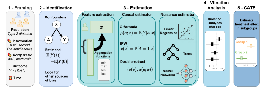
Figure 1: Step-by-step analytic framework – The complete inference pipeline confronts the analyst with many choices, some guided by domain knowledge, others by data insights. Making those choices explicit is necessary to ensure robustness and reproducibility.

2.1 Step 1: study design – Frame the question to avoid biases

PICO component	Description	Notation	Example
Population	What is the target population of interest?	$X\sim\mathbb{P}(X)$, the covariate distribution	Patients with sepsis in the ICU
Intervention	What is the treatment?	$A\sim\mathbb{P}(A=1)=p_{A}$, the probability to be treated	Combination of crystalloids and albumin
Control	What is the clinically relevant comparator?	$1-A\sim 1-p_{A}$	Crystalloids only
Outcome	What are the outcomes to compare?	$Y(1),Y(0)\sim\mathbb{P}(Y(1),Y(0))$, the potential outcomes distribution	28-day mortality
Time	Is the start of follow-up aligned with intervention assignment?	N/A	Intervention administered within the first 24 hours of admission

Table 1: PICO(T) components help to clearly define the medical question of interest.

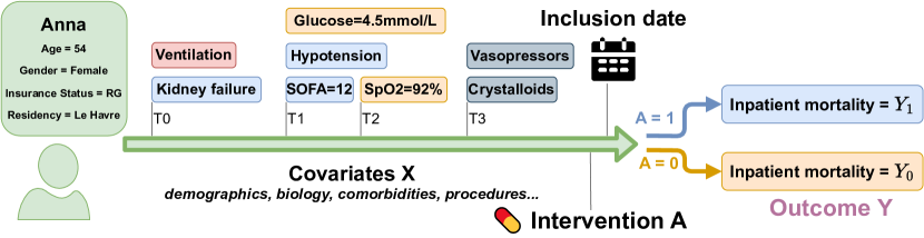
Figure 2: Study design – The first step of the analysis consists in identifying a valid treatment effect question from patient healthcare trajectories and defining a target trial emulating a RCT using the PICO(T) framework.

Grounding decisions on evidence needs well-framed questions, defined by their PICO components: Population, Intervention, Control, and Outcome [91]. To concord with a (hypothetical) target randomized clinical trial, an analysis must emulate all these components [43, 128], eg via potential outcome statistical framework [42] –Table 1 and Figure 2. EHRs and Claims need an additional time component: PICOT [93].

Without dedicated care, defining those PICO(T) components from EHRs can pick up bias: non-causal associations between treatment and outcomes. We detail two common sources of bias in the Population and Time components: selection bias and immortal time bias, respectively.

Selection Bias:

In EHRs, outcomes and treatments are often not directly available and need to be inferred from indirect events. These signals could be missing not-at random, sometimes correlated with the treatment allocation [130]. For example, not all billing codes are equally well filled in, as billing is strongly associated with case-severity and cost. Consider comparing the effect on mortality of fluid resuscitation with albumin to that of crystalloids. As albumin is much more costly, patients who have received this treatment are much more likely to have a sepsis billing code, independent of the seriousness of their condition. On the contrary, for patients treated with crystalloids, only the most severe cases will have a billing code. Naively comparing patients on crystalloid treatment with less sick patients on albumin treatment would overestimate the effect of albumin.

Immortal time bias:

Another common bias comes from timing: improper alignment of the inclusion defining event and the intervention time [118, 41, 129]. Figure 3 illustrates this Immortal time bias –related to survivor bias [59]. It occurs when the follow-up period, i.e. cohort entry, starts before the intervention, e.g. prescription for a second-line treatment. In this case, the treated group will be biased towards patients still alive at the time of assignment and thus overestimating the effect size. Other common temporal biases are lead time bias [79, 32], right censorship [41], and attrition bias [9].

Good practices include explicitly stating the cohort inclusion event [78, Chapter 10:Defining Cohorts] and defining an appropriate grace period between starting time and the intervention assignment [41]. At this step, a population timeline can help (eg. Figure 5).

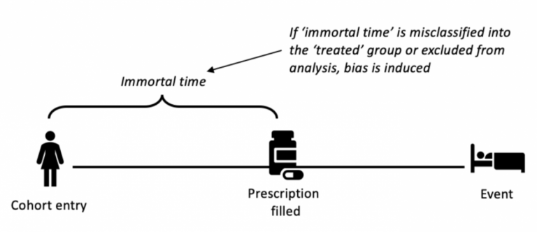
Figure 3: Poor experimental design can introduce Immortal time bias, which leads to a treated group with falsely longer longevity [59].

2.2 Step 2: identification – List necessary information to answer the causal question

The identification step builds a causal model to answer the research question (Figure 6). Indeed, the analysis must compensate for differences between treated and non-treated that are not due to the intervention ([83, chapter 1], [42, chapter 1]).

Causal Assumptions

Not every question can be answered from a given dataset: valid causal inference requires assumptions [101] –detailed in Appendix D. The analyst should thus review the plausibility of the following: 1) Unconfoundedness: after adjusting for the confounders as ascertained by domain expert insight, treatment allocation should be random; 2) Overlap –also called positivity– the distribution of confounding variables overlaps between the treated and controls –this is the only assumption testable from data [7]–; 3) No interference between units and a constant version of the treatment, a reasonable assumption in most clinical questions.

Categorizing covariates

Potential predictors –covariates– should be categorized depending on their causal relations with the intervention and the outcome (Figure 4): confounders are common causes of the intervention and the outcome; colliders are caused by both the intervention and the outcome; instrumental variables are a cause of the intervention but not the outcome, mediators are caused by the intervention and is a cause of the outcome. Finally, effect modifiers interact with the treatment, and thus modulate the treatment effect in subpopulations [6].

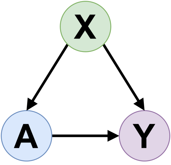
Confounder

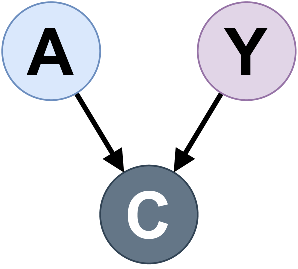
Collider

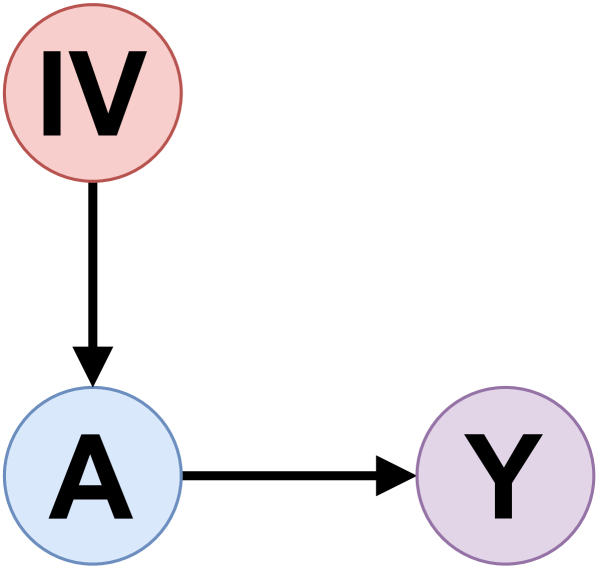
Instrumental variable

Mediator

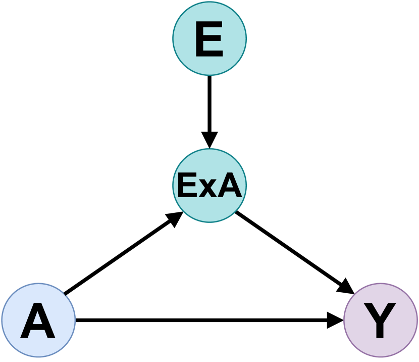
A: Treatment Y: Outcome X: Confounder C: Collider IV: Instrumental variable M: Mediator E: Effect modifier

Effect modifier
[6, Represented following]

Figure 4: The five categories of causal variables needed for our framework.

To capture a valid causal effect, the analysis should only include confounders and possible treatment-effect modifiers to study the resulting heterogeneity. Regressing the outcome on instrumental and post-treatment variables (colliders and mediators) will lead to biased causal estimates [124]. Drawing causal Directed Acyclic Graphs (DAGs) [38], eg with a webtool such as DAGitty [119], helps capturing the relevant variables from domain expertise.

Estimand or effect measure

The estimand is the final statistical quantity estimated from the data. Depending on the question, different estimands are better suited to contrast the two potential outcomes E[Y(1)] and E[Y(0)] [50, 20]. For continuous outcomes, risk difference is a natural estimand, while for binary outcomes (e.g. events) the choice of estimand depends on the scale of the study. Whereas the risk difference is very informative at the population level, e.g. for medico-economic decision making, the risk ratio and the hazard ratio are more informative to reason on sub-populations such as individuals or sub-groups [20].

2.3 Step 3: Estimation – Compute the causal effect of interest

Confounder aggregation

Some confounders are captured via measures collected over multiple time points. These need to be aggregated at the patient level. Simple forms of aggregation include taking the first or last value before a time point, or an aggregate such as mean or median over time. More elaborate choices may rely on hourly aggregations of information such as vital signs. These provide more detailed information on the health evolution, thus reducing confounding bias between rapidly deteriorating and stable patients. However, it also increases the number of confounders, resulting in a larger covariate space, hence increasing the estimate’s variance and endangering the positivity assumption. The choices should be guided by expert knowledge. If multiple choices appear reasonable, one should compare them in a vibration analysis (see Section 2.4). Indeed, aggregation may impact results, as [114] show, revealing that some choices of averaging time scale lead to inconclusive links between HbA1c levels and survival in diabetes.

Beyond measures and clinical codes, unstructured clinical text may capture confounding or prognostic information [47, 54] which can be added in the causal model [136].

Causal estimators or statistical modeling

A given estimand can be estimated through different methods. One can model the outcome with regression models [95, also known as G-formula,] and use it as a predictive counterfactual model for all possible treatments for a given patient. Alternatively, one can model the propensity of being treated use it for matching or Inverse Propensity Weighting (IPW) [7]. Finally, doubly robust methods model both the outcome and the treatment, benefiting from the convergence of both models [125]. Various doubly robust models have emerged: Augmented Inverse Propensity Score (AIPW) [96], Double Robust Machine Learning [18], or Targeted Maximum Likelihood Estimation (TMLE) [106] to name a few (details in Appendix E.1).

Estimation models of outcome and treatment

The causal estimators use models of the outcome or the treatment –called nuisances as they are not the main inference targets in our causal effect estimation problem. Which statistical model is best suited is an additional choice and there is currently no clear best practice [131, 25]. The trade-off lies between simple models risking misspecification of the nuisance parameters versus flexible models risking to overfit the data at small sample sizes. Stacking models of different complexity in a super-learner is a good solution to navigate the trade-off [123, 26].

2.4 Step 4: Vibration analysis – Assess the robustness of the hypotheses

Some choices in the pipeline may not be clear cut. Several options should then be explored, to derive conceptual error bars going beyond a single statistical model. This process is sometimes called robustness analysis [76] or sensitivity analysis [120, 42, 29]. However, in epidemiology, sensitivity analysis refers to quantifying the bias from unobserved confounders [103]. Following [82], we use the term vibration analysis to describe the sensitivity of the results to all analytic choices. The vibration analysis can identify analytic choices that deserve extra scrutiny. It complements a comparison to previous studies –ideally RCTs– to establish the validity of the pipeline.

2.5 Step 5: Treatment heterogeneity – Compute treatment effects on subpopulations

Once the causal design and corresponding estimators are established, they can be used to explore the variation of treatment effects among subgroups. Measures of the heterogeneity of a treatment nourish decisions tailored to a patient’s characteristics. A causally-grounded model, eg using machine learning, can be used to predict the effect of the treatment from all the covariates –confounders and effect modifers– for an individual: the Individual Treatment Effect [65, ITE]. Studying heterogeneity only along specific covariates, or a given patient stratification, is related to the Conditional Average Treatment Effect (CATE) [94]. Practically, CATEs can be estimated by regressing the individual predictions given by the causal estimator against the sources of heterogeneity (details in L.3).

3 Application: evidence from MIMIC-IV on which resuscitation fluid to use

We now use the above framework to extract evidence-based decision rules for resuscitation. Ensuring optimal organ perfusion in patients with septic shock requires resuscitation by reestablishing circulatory volume with intravenous fluids. While crystalloids are readily available, inexpensive and safe, a large fraction of the administered volume is not retained in the vasculature. Colloids offer the theoretical benefit of retaining more volume in the circulation, but might be more costly and have adverse effects [5]. The scientific community long debated which fluid benefits patients most [68].

Emulated trial: Effect of albumin in combination with crystalloids compared to crystalloids alone on 28-day mortality in patients with sepsis

We illustrate the impact of the different analytical steps to conclude on the effect of albumin in combination with crystalloids compared to crystalloids alone on 28-day mortality in patients with sepsis using MIMIC-IV [55]. This question is clinically relevant and multiple published RCTs can validate the average treatment effect. Appendix C provides further examples of potential target trials.

Evidence from the literature

Meta-analyses from multiple pivotal RCTs found no effect of adding albumin to crystalloids [61] on 28-day and 90-day mortality. Further, an observational study in MIMIC-IV [137] found no significant benefit of albumin on 90-day mortality for severe sepsis patients. Given this previous evidence, we thus expect no average effect of albumin on mortality in sepsis patients. However, studies –RCT [15] and observational [61]– have found that septic-shock patients do benefit from albumin.

3.1 Study design: effect of crystalloids on mortality in sepsis

• Population: Patients with sepsis within the ICU stay according to the sepsis-3 definition. Other inclusion criteria: sufficient follow-up of at least 24 hours, and age over 18 years described in table 2.

• Intervention: Treatment with a combination of crystalloids and albumin during the first 24 hours of an ICU stay.

• Control: Treatment with crystalloids only in the first 24 hours of an ICU stay.

• Outcome: 28-day mortality.

• Time: Follow-up begins after the first administration of crystalloids. Thus, we potentially introduce a small immortal time bias by allowing a time gap between follow-up and the start of the albumin treatment –shown in Figure 5. Because we are only considering the first 24 hours of an ICU stay, we hypothesize that this gap is insufficient to affect our results. We test this hypothesis in the vibration analysis step.

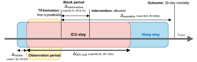
Figure 5: Defining the inclusion event, the starting time T0 for follow-up, the intervention’s assignment time and the observation window for confounders is crucial to avoid time and selection biases. In our study, the gap between the intervention and the inclusion is small compared to the occurrence of the outcome to limit immortal time bias: 6.7 hours vs 40 days for mortality.

In MIMIC-IV, these inclusion criteria yield 18,121 patients with 3,559 patients treated with a combination of crystalloids and albumin (Appendix G details the selection flowchart).

3.2 Identification: listing confounders

We enrich the confounders selection procedure described by [137] with expert knowledge, creating the causal DAG shown in Figure 6. Gray confounders are not controlled for, since they are not available in the data. However, resulting confounding biases are captured by proxies such as comorbidity scores (SOFA or SAPS II) or other variables (eg. race, gender, age, weight). Appendix H details confounders summary statistics for treated and controls.

	Missing	Overall	Cristalloids only	Cristalloids + Albumin	P-Value
n		18421	14862	3559
Female, n (%)		7653 (41.5)	6322 (42.5)	1331 (37.4)
White, n (%)		12366 (67.1)	9808 (66.0)	2558 (71.9)
Emergency admission, n (%)		9605 (52.1)	8512 (57.3)	1093 (30.7)
admission_age, mean (SD)	0	66.3 (16.2)	66.1 (16.8)	67.3 (13.1)	<0.001
SOFA, mean (SD)	0	6.0 (3.5)	5.7 (3.4)	6.9 (3.6)	<0.001
lactate, mean (SD)	4616	3.0 (2.5)	2.8 (2.4)	3.7 (2.6)	<0.001

Table 2: Characteristics of the trial population measured on the first 24 hours of ICU stay. Appendix 8 describes all confounders used in the analysis.

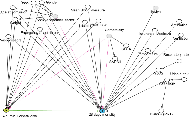
Figure 6: Causal graph for the Albumin vs crystalloids emulated trial – The green arrow indicates the effect studied. Black arrows show causal links known to medical expertise. Dotted red arrows highlight confounders not directly observed. For readability, we draw only the most important edges from an expert point of view. All white nodes corresponds to variables included in our study.

3.3 Estimation

Confounder aggregation:

We tested multiple aggregations such as the last value before the start of the follow-up period, the first observed value, and both the first and last values as separated features.

Causal estimators:

We implemented multiple estimation strategies, including Inverse Propensity Weighting (IPW), outcome modeling (G-formula) with T-Learner, Augmented Inverse Propensity Weighting (AIPW) and Double Machine Learning (DML). We used the python packages dowhy [110] for IPW implementation and EconML [10] for all other estimation strategies. Confidence intervals were estimated by bootstrap (50 repetitions). Appendices E.1 and E.3 detail the estimators and the available Python implementations.

Outcome and treatment estimators:

To model the outcome and treatment, we used two common but different estimators: random forests and ridge logistic regression implemented with scikit-learn [84]. We chose the hyperparameters with a random search procedure (detailed in Appendix E.4). While logistic regression handles predictors in a linear fashion, random forests should have the benefit of modeling non-linear relations as well.

3.4 Vibration analysis: Understanding variance or sources of systematic errors in our study

Varying estimation choices: Confounders aggregation, causal and nuisance estimators:

Figure 7 shows varying confidence intervals (CI) depending on the method. Doubly-robust methods provide the narrowest CIs, whereas the outcome-regression methods have the largest CI. The estimates of the forest models are closer to the consensus across prior studies (no effect) than the estimates from the logistic regression indicating a better fit of the non-linear relationships in the data. We only report the first and last pre-treatment feature aggregation strategies, since detailed analysis showed little differences for other choices of feature aggregation (see Appendix I). Confronting this analysis with the prior published evidence of little-to-no effect, it seems reasonable to select the models using random forests for nuisance. Out of these, theory suggests to trust more double machine learning or doubly robust approaches.

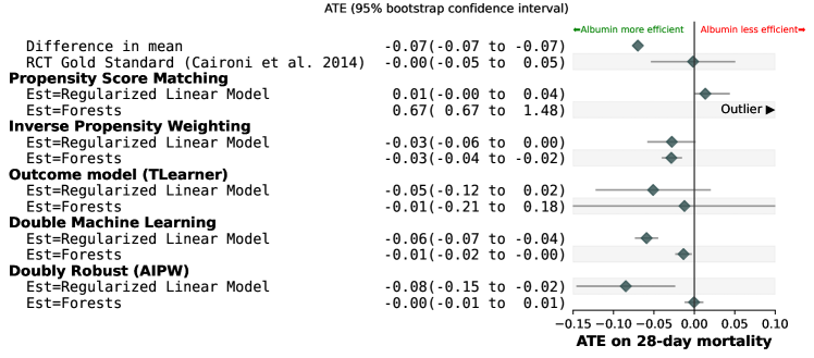
Figure 7: Forest plot for the vibration analysis – Different estimators give different results, sometimes even outside of each-other’s bootstrap confidence intervals. Score matching yields unconvincingly high estimates, inconsistent with the published RCT. With other causal approaches, using linear estimators for nuisances suggest a reduced mortality risk for albumin, while using forests for nuisance models points to no effect, which is consistent with the RCT gold standard. The diamonds depict the mean effect and the bar are the 95% confidence intervals obtained by 50 bootstrap repetitions.

Study design – Illustration of immortal time bias:

To illustrate the risk of immortal-time bias, we varied the eligibility period by allowing patients to receive the treatment or the control in a shorter or longer time window than 24 hours. As explained in subsection 2.1, a large eligibility period means that patients in the study are more likely to be treated if they survived till the intervention and hence the study is biased to overestimate the beneficial effect of the intervention. Figure 8 shows that larger eligibility periods change the direction of the estimate and lead to Albumin seeming markedly more efficient. Should the analyst not have in mind the mechanism of immortal time bias, this vibration analysis ought to raise an alarm and hopefully lead to correct the study design.

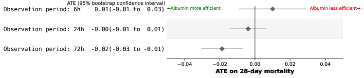
Figure 8: Detecting immortal time bias – Increasing the observation period increases the temporal blank period between inclusion and treatment initialization, associating thus patients surviving longer with treatment: Immortal Time Bias. A longer observation period (72h) artificially favors the efficacy of Albumin. The estimator is a doubly robust learner (AIPW) with random forests for nuisances. This result is consistent across estimators as shown in Appendix J. The green diamonds depict the mean effect and the bar are the 95% confidence intervals obtained by 30 bootstrap repetitions.

3.5 Treatment heterogeneity: Which treatment for a given sub-population?

We now study treatment heterogeneity using the pipeline validated by confronting the vibration analysis to the literature: a study design avoiding immortal time bias, and the double machine learning model using forest for nuisances and a linear model for the final heterogeneity regression. We explore heterogeneity along four binary patient characteristics, displayed on Figure 9. We find that albumin is beneficial with patient with septic shock before fluid administration, consistent with the [15] RCT. It is also beneficial for older patients (age >=60) and males, consistent with [137], as well as white patients.

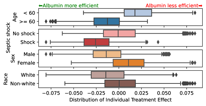
Figure 9: The subgroup distributions of Individual Treatment effects showed better treatment efficacy for patients older than 60 years, septic shock, and to a lower extent males. The final estimator is ridge regression. The boxes contain the $25^{\text{th}}$ and $75^{\text{th}}$ percentiles of the CATE distributions with the median indicated by the vertical line. The whiskers extend to 1.5 times the inter-quartile range of the distribution.

4 Discussion and conclusion

Our analytic framework strives to streamline extracting valid decision-making rules from EHR data. Decision-making is tied to a choice: to treat or not to treat, for a given intervention. A major pitfall, source of numerous shortcuts of machine-learning systems, is to extract non-causal associations between the intervention and the outcome. Our framework is designed to avoid these pitfalls by starting with rigorous causal analysis, in the form of a target trial, to validate study design and analytic choices before more elaborate analysis, potentially using machine-learning for individual predictions. We argue that in the absence of a precise framing including treatment allocation, automated decision making is brittle. It is all too easy, for instance, to build a predictive system on post-treatment data, rendering it unreliable for decision making. EHR data come with particular challenges: information may be available indirectly, e.g. via billing codes, the time-wise dimension requires aggregations (subsection 2.3). These challenges can create subtle causal biases (subsection 2.1). To ensure that our framework addresses all aspects of EHR analysis and to expose it in a didactic way, we detailed a complete analysis of a publicly-available EHR dataset, supported by open code.

A well-framed target trial can be validated

Assessing the validity of an analysis is challenging even for experts [52, 14]. Our framework recommends using a well-specific target trial to establish a valid pipeline because it helps confronting the resulting average treatment effect to other evidence [43, 128]. Our resuscitation-fluid analysis matches well published findings: Pooling evidence from high-quality RCTs, no effect of albumin in severe sepsis was demonstrated for both 28-day mortality (odds ratio (OR) 0.93, 95% CI 0.80-1.08) and 90-day mortality (OR 0.88, 95% CI 0.76-1.01) [133]. This consistency validates our study design and analytic choices. Varying analytic choices and confronting them to prior studies can reveal loopholes in the analysis, as we demonstrated with immortal time bias: extending the time between ICU admission and intervention to 72 hours, we observed an inflation of effect size consistent with such bias. Looping back to reference RCTs reveals that these include patients within 8 to 24 hours of ICU admission [102, 5, 15].

Decision-making from EHRs

Once the causal analysis has been validated, it can be used for decision making. A sub-population analysis (as in Figure 9) can distill rules on which groups of patients should receive the treatment. Ideally, dedicated RCTs can be run with inclusion criteria matching these sub-groups. However, the cost and the ethical concerns of running RCTs limit the number of sub-groups that can be explored. In addition, the sub-group view risks oversimplifying, as opposed to patient-specific effect estimates to support more individualized clinical decision making [57]. For this, predictive modeling shines. Causally-grounded machine learning can give good counter-factual prediction [86, 40, 92], if it predicts well the treated and untreated outcomes [26]. Even without focusing on a specific intervention, anchoring machine learning on causal mechanisms gives models that are more robust to distributional shift [105], safer for clinical use [92], and more fair [85]. Capturing individualized effects via machine-learning models does require to probe many diverse individuals. EHRs and claims data are well suited for these models, as they easily cover much more individuals than a typical clinical study.

But EHRs cannot inform on trade-offs that have not been explored in the data. No matter how sophisticated, causal inference cannot conclude if there is no data to support an apple-to-apple comparison between treated and non-treated individuals. For example, treatment allocation is known to be influenced by race- and gender-concordance between the patient and the care provider. Yet, if the EHR data does no contain this information, it cannot nourish evidence-based decisions on such matter. EHRs and RCTs complement each other: a dedicated study, with a randomized intervention, as an RCT, can be crafted to answer a given question on a given population. But RCTs cannot address all the subpopulations, local practices, healthcare systems [100, 121, 56]. Our framework suggest to integrate the evidence from RCTs designed with matching PICO formulation to ensure the validity of the analysis and to use the EHR to explore heterogeneity.

Conclusion

Without causal thinking machine learning does not suffice for optimal clinical decision making for each and every patient. It will replicate non-causal associations such as shortcuts improper for decision making. As models can pick up information such as race implicitly from the data [2], they risk propagating biases when building AI models which can further reinforce health disparities. This problem is acknowledged by the major tech companies which are deploying causal inference tooling to mitigate biases [37, 70, 87]. On the medical side, causal modeling can create actionable decision-making systems that reduce inequities [71, 27]. However, as we have seen, subtle errors can make an intervention seemingly more –or less– beneficial to patients. No sophisticated data-processing tool can safeguard against invalid study design or modeling choices. The goal of our step-by-step analytic framework is to help the data analyst work around these loopholes, building models that avoid shortcuts and extract the best decision-making evidence. Applied to study the addition of albumin to crystalloids to resuscitate sepsis patients, it shows that this addition is not beneficial in general, but that it does improve survival on specific individuals, such as patients undergoing sceptic shock.

Availability of data and materials

The datasets are available on PhysioNet ( https://doi.org/10.13026/6mm1-ek67). We used MIMIC-IV.v2.2 The code for data preprocessing and analyses are available on github https://github.com/soda-inria/causal_ehr_mimic/.

Fundings

This study was supported by an unrestricted educational grants to TS (Swiss National Science Foundation, P400PM_194497 / 1) as well as an ERC grant to GV (Intercept-T2D HORIZON-HLTH-2022-STAYHLTH-02-01).

Authors contributions

MD and TS designed the study, MD performed the analysis and wrote the manuscript. TS, JA, CM, LAC, GV reviewed and edited the manuscript.

Competing interests

All authors declare no financial or non-financial competing interests.

Appendix A Motivating example: Failure of predictive models to predict mortality from pretreatment variables

To illustrate how machine learning frameworks can fail to inform decision making, we present a motivating example from MIMIC-IV. Using the same population and covariates as in the main analysis (described in Table 8), we train a predictive model for 28-day mortality. We split the data into a training set (80%) and a test set (20%). The training set uses the last measurements from the first 24 hours, whereas the validation set only uses the last measurements before the administration of crystalloids. We split the train set into a train and a validation set. We fit a HistGradientBoosting classifier on the train set and evaluate the performance on the validation set and on the test set. We see good area under the Precision-recall curve (PR AUC) on the validation set, but a deterioration of 10 points on the test set (Figure 10(a)). The same is seen in Figure 10(b) when measuring performance with Area Under the Curve of the Receiving Operator Characteristic (ROC AUC). In the contrary, a model trained on pre-treatment features yield competitive performances. This failure illustrates well the shortcuts on which predictive models could rely to make predictions. A clinically useful predictive model should support decision making –in this case, addition of albumin to crystalloids– rather than maximizing predictive performance. In this example, causal thinking would have helped to identify the bias introduced by post-treatment features. In fact, these features should not be included in a causal analysis since they are post-treatment colliders.

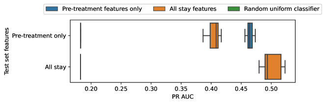
(a)

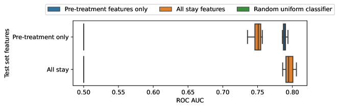
(b)

Figure 10: Failure to predict 28-day mortality from a model fitted on pre-treatment variables. The model is trained on the last features from the whole stay and tested on two validation sets: one with all stay features and one with last features before crystalloids administration (Pre-treatment only). The all-stay model performance markedly decreases in the pre-treatment only dataset.

Appendix B Estimation of Treatment effect with MIMIC data

We searched for causal inference studies in MIMIC using PubMed and Google scholar with the following search terms ((MIMIC-III OR MIMIC-IV) AND (causal inference OR treatment effect)). We retained eleven treatment effect studies clearly following the PICO framework:

• [63] studied the effect of High-flow nasal cannula oxygen (HFNC) against noninvasive mechanical ventilation on 801 patients with hypoxemia during ventilator weaning on 28-day mortality. They used propensity score matching, and found non-negative effects as previous RCTs reported – though those were focused on reintubation as the main outcome [115, 44].

• [135] studied the effect of lower hypoxemia vs higher hypoxemia thresholds for the initiation of invasive ventilation (defined with saturation-to-inspired oxygen ratio (SF)) for 3,357 patients from MIMIC receiving inspired oxygen fraction >= 0.4 on 28-day moratlity. Using bayesian G-computation (time-varying treatment model with gaussian process and outcome-model with BART, taking the treatment model as entry), they found protective effects for initialization at low hypoxemia. However, when externally validation their findings in the AmsterdamUMCdb dataset, they found the highest mortality probability for patients with low hypoxemia. Authors concluded that their model was heavily dependent on clinical context and baseline caracteristics. There might be some starting-time bias in this study since it is really close

• [48] studied the effect of indwelling arterial catheters (IACs) vs non-IAC for 1,776 patients who are mechanically ventilated and did not require vasopressor support on 28-day mortality. They used propensity score matching and found no effect. A notebook based on google cloud access to MIMIC-IV replicating the study is available here.

• [30] studied the effect of transthoracic echocardiography vs no intervention for 6,361 patients with sepsis on 28-day mortality. They used IPW, PSM, g-formula and a doubly robust estimation. The propensity score was modeled with boosting and the outcome model with a logistic regression. They found a significant positive reduction of mortality (odd ratio 0.78, 95% CI 0.68-0.90). Study code is open source.

• [33] studied the effect of liberal –target SpO2 greater than 96%– vs conservative oxygenation –target SpO2 between 88-95%– in 4,062 mechanically ventilated patients on 90-day mortality. They found an advantage of the liberal strategy over liberal (ATE=0.13) by adjusting on age and apsii. This is not consistent with previous RCTs where no effects have been reported [80, 66].

• [108] studied the effect of fluid-limiting treatment –caped between 6 and 10 L– vs no cap on fluid administration strategies for 1,639 sepsis patients on 30 day-mortality. Using a dynamic Marginal Structural Model with IPW, they found a protective effect of fluid-limitation on ATE -0.01 (95%CI -0.016, -0.03). This is somehow concordant with the RIFTS RCT that found no effect of fluid limitation [21] and two previous meta-analyses [67, 69].

• [19] studied the effect of statin use prior to ICU admission vs absence of pre-ICU prescription for 8,200 patients with sepsis on 30-day mortality. Using AIPW (no estimator reported) and PSM (logistic regression), they found a decrease on mortality (ATE -0.039, 95%CI -0.084, -0.026). This partly supports previous findings in Propensity Matching bases observational studies [60, 58]. But all RCTs [75, 112] found no improvement for sepsis (not pre-admission administration though). The [126] meta-analysis concludes that there is lack of evidence for the use of statins in sepsis with inconsistent results between RCTs (no effect) and observational studies (protective effect).

• [3] studied the effect of higher vs lower positive end-expiratory pressures (PEEP) in 1,411 patients with Acute Respiratory Distress Syndrome (ARDS) syndrome on 30 day mortality. Very few details on the methods were reported, but they found a protective effect for higher PEEP consistent results from a target trial [74].

• [3] also studied the effect of early use of a neuromuscular blocking agent vs placebo in 752 patients moderate-severe ARDS on 30 day mortality. Very few details on the methods were reported, but they found a protective effect for the use of a neuromuscular blocking agent, consistent with the results from a target trial [81].

• [137] studied the administration of a combination of albumin within the first 24-h after crystalloids vs crystalloids alone for 6,641 patients with sepsis on 28-day mortality. Using PSM, they found protective effect of combination on mortality, but insist on the importance of initialization timing. This is consistent with [133], who found a non-significant trend in favor of albumin used for severe sepsis patients and a significant reduction for septic shock patients, both on 90-day mortality. These results are aligned with [15] that found no effect for severe sepsis patient but positive effect for septic shock patients.

• [127] studied early enteral nutrition (EN) –<=53 ICU admission hours– vs delayed EN for 2,364 patients with sepsis and EN on acute kidney injury. With PSM, IPW and g-formula (logistic estimator each time), they found a protective effect (OR 0.319, 95%CI 0.245, 0.413) of EEN.

These eleven studies mainly used propensity score matching (6) and IPW (4), two of them used Double robust methods, and only one included a non-linear estimator in either the outcome or the treatment model. None of them performed a vibration analysis on the confounders selection or the feature transformations. They have a strong focus on sepsis patients. Only four of them found concordant results with previous RCTs [63, 108, 3].

Appendix C Target trials proposal suitable to be replicated in MIMIC

[17] suggested the creation of a causal inference database based on MIMIC with a list of replicable RCTs, which has not been accomplished yet. We reviewed the following RCTs, which could be replicated within the MIMIC-IV database. Table 4 details the sample sizes of the eligible, control and treated populations for the identified RCTs.

Trial name	Criteria description	Number of patients	Criteria status	Implemented	Target RCT or meta-analysis reference
Fludrocortisone combination for sepsis	Septic shock defined by the sepsis-3 criteria, first stay, over 18, not deceased during first 24 hours of ICU	28,763	target population	✓	[134]
	Hydrocortisone administred and sepsis	1,855	control	✓
	Both corticoides administered and sepsis	153	intervention	✓
High flow oxygen therapy for hypoxemia	Over 18, hypoxemia 4 h before planed extubation (PaO2, FiO2) $\leq$ 300 mmHg), and either High Flow Nasal Cannula (HFNC) or Non Invasive Ventilation (NIV)	801	target population	✗	[115], [43]
	Eligible hypoxemia and HFNC	358	intervention	✗
	Eligible hypoxemia and NIV	443	control	✗
Routine oxygen for myocardial infarction	Myocardial infarction without hypoxemia at admission: - Myocardial infarction defined with ICD9-10 codes, first stay, over 18, not deceased during first 24 hours of ICU - Hypoxemia during first 2 hours defined as either (PaO2/FiO2) $leq$ 300mmHg OR SO2 $leq$ 90 OR SpO2 $\leq$ 90	3,379	target population	✓	[46], [116]
	Myocardial infarction without hypoxemia at admission AND Supplemental Oxygen OR Non Invasive Vent	1,901	intervention	✓
	Myocardial infarction without hypoxemia at admission AND no ventilation of any kind during first 12 hours	605	control	✓
Prone positioning for ARDS	Acute Respiratory Distress Syndrome (ARDS) during the first 12 hours defined as (PaO2,FiO2) $leq$ 300mmHg, first stay, over 18, not deceased during 24 hours of ICU	11506	trial population	✓	[73]
	Prone positioning and ARDS	547	intervention	✓
	Supline position and no prone position	10,904	control	✓
NMBA for ARDS	ARDS during the first 12 hours defined as (PaO2,FiO2) $leq$ 300mmHg, first stay, over 18, not deceased during 24 hours of ICU	11,506	trial population	✓	[81], [45]
	Neuromuscular blocking agent (NBMA) as cisatracurium injections during the stay.	709	intervention	✓
	No NBMA during the stay	10,797	control	✓
Albumin for sepsis	Septic shock defined by the sepsis-3 criteria, first stay, over 18, not deceased during first 24 hours of ICU, having crystalloids	18,421	trial population	✓	[15], [61], [122]
	Sepsis-3 and crystalloids during first 24h, no albumin	14,862	control	✓
	Sepsis-3 and combination of crystalloids followed by albumin during first 24h	3,559	intervention	✓

Table 3:

Table 4: Eligibility criteria and resulting populations for potential target trials in MIMIC-IV.

Appendix D Assumptions: what is needed for causal inference from observational studies

The following four assumptions, referred as strong ignorability, are needed to assure identifiability of the causal estimands with observational data with most causal-inference methods [101], in particular these we use:

Assumption 1 (Unconfoundedness)

$$\{Y(0),Y(1)\}\perp\!\!\!\perp A|X$$ (1)

This condition –also called ignorability– is equivalent to the conditional independence on the propensity score $e(X)=\mathbb{P}(A=1|X)$ [99]: $\{Y(0),Y(1)\}\perp\!\!\!\perp A|e(X)$.

Assumption 2 (Overlap, also known as Positivity)

$$\eta<e(x)<1-\eta\quad\forall x\in\mathcal{X}\text{ and some }\eta>0$$ (2)

The treatment is not perfectly predictable. Or in other words, every patient has a chance to be treated and not to be treated. For a given set of covariates, we need examples of both to recover the ATE.

As noted by [22], the choice of covariates $X$ can be viewed as a trade-off between these two central assumptions. A bigger covariate set generally reinforces the ignorability assumption. In the contrary, overlap can be weakened by large $\mathcal{X}$ because of the potential inclusion of instrumental variables: variables only linked to the treatment which could lead to arbitrarily small propensity scores.

Assumption 3 (Consistency)

The observed outcome is the potential outcome of the assigned treatment:

$$Y=A\,Y(1)+(1-A)\,Y(0)$$ (3)

Here, we assume that the intervention $A$ has been well defined. This assumption focuses on the design of the experiment. It clearly states the link between the observed outcome and the potential outcomes through the intervention [42].

Assumption 4 (Generalization)

The training data on which we build the estimator and the test data on which we make the estimation are drawn from the same distribution, also known as the “no covariate shift” assumption [53].

Appendix E Major causal-inference methods

E.1 Causal estimators: When to use which method ?

G-formula

also called conditional mean regression [131], g-computation [95], or Q-model [113]. This approach is directly modeling the outcome, also referred to as the response surface: $\mu_{(a)}(x)=\mathbb{E}\left(Y\mid A=a,\mathbf{X}=x\right)$

Using an outcome estimator to learn a model for the response surface $\hat{\mu}$ (eg. a linear model), the ATE estimator is an average over the n samples:

$$\hat{\tau}_{G}(f)=\frac{1}{n}\sum_{i=1}^{n}\hat{\mu}(x_{i},1)-\hat{\mu}(x_{i},0)=\frac{1}{n}\sum_{i=1}^{n}\hat{\mu}_{(1)}(x_{i})-\hat{\mu}_{(0)}(x_{i})$$ (4)

This estimator is unbiased if the model of the conditional response surface $\hat{\mu}_{(a)}$ is well-specified. This approach assumes than $Y(a)=\mu_{a}(X)+\epsilon_{a}$ with $\mathbb{E}[\epsilon|X]=0$. The main drawback is the extrapolation of the learned outcome estimator from samples with similar covariates X but different intervention A.

Propensity Score Matching (PSM)

To avoid confounding bias, the ignorability assumption 1) requires to contrast treated and control outcomes only between comparable patients with respect to treatment allocation probabilities. A simple way to do this is to group patients into bins, or subgroups, of similar confounders and contrast the two population outcomes by matching patients inside of these bins [117]. However, the number of confounder bins grows exponentially with the number of variables. [99] proved that matching patients on the individual probabilities to receive treatment –propensity scores– is sufficient to verify ignorability. PSM is a conceptually simple method, but has delicate parameters to tune such as choosing a model for the propensity score, deciding what is the maximum distance between two potential matches (the caliper width), the number of matches by sample, and matching with or without replacement. It also prunes data not meeting the caliper width criteria, and suffers form high estimation variance in highly-dimensional data where extreme propensity weights are common. Finally, the simple bootstrap confidence intervals are not theoretically grounded [1], making PSM more difficult to use for applied practitioners.

Inverse Propensity Weighting (IPW)

A simple alternative to propensity score matching is to weight the outcome by the inverse of the propensity score: Inverse Propensity Weighting [7]. It relies on the same idea than matching but builds automatically balanced population by reweighting the outcomes with the propensity score model $\hat{e}$ to estimate the ATE:

$$\hat{\tau}_{IPW}(\hat{e})=\frac{1}{n}\sum_{i=1}^{N}\frac{A_{i}Y_{i}}{\hat{e}(X_{i})}-\frac{(1-A_{i})Y_{i}}{(1-\hat{e}(X_{i}))}$$ (5)

This estimate is unbiased if $\hat{e}$ is well-specified. IPW suffers from high variance if some weights are too close to 0 or 1. In high-dimensional cases where poor overlap between treated and control is common, one can clip extreme weights to limit estimation instability.

Doubly Robust Learning, DRL

also called Augmented Inverse Probability Weighting (AIPW) [96].

The underlying idea of DRL is to combine the G-formula and IPW estimators to protect against a mis-specification of one of them. It first requires to estimate the two nuisance parameters: a model for the intervention $\hat{e}$ and a model for the outcome $f$. If one of the two nuisance is unbiased, the following ATE estimator is as well:

$$\widehat{\tau}_{AIPW}=\frac{1}{n}\sum_{i=1}^{n}\left(\hat{\mu}_{(1)}\left(x_{i}\right)-\hat{\mu}_{(0)}\left(x_{i}\right)+a_{i}\frac{y_{i}-\hat{\mu}_{(1)}\left(x_{i}\right)}{\hat{e}\left(x_{i}\right)}-\left(1-a_{i}\right)\frac{y_{i}-\hat{\mu}_{(0)}\left(x_{i}\right)}{1-\hat{e}\left(x_{i}\right)}\right)$$

Moreover, despite the need to estimate two models, this estimator is more efficient in the sense that it converges quicker than single model estimators [125]. For this propriety to hold, one need to fit and apply the two nuisance models in a cross-fitting manner. This means that we split the data into K folds. Then for each fold, we fit the nuisance models on the K-1 complementary folds, and predict on the remaining fold.

To recover Conditional Treatment Effects from the AIPW estimator, [31] suggested to regress the Individual Treatment Effect estimates from AIPW on potential sources of heterogeneity $X^{cate}$: $\hat{t}au=\operatorname*{arg\,min}_{\tau\in\Theta}(\hat{\tau}_{AIPW}(X)-\tau(X^{cate}))$ for $\Theta$ some class of model (eg. linear model).

Double Machine Learning

[18] also known as the R-learner [77]. It is based on the R-decomposition, [97], and the modeling of the conditional mean outcome, $m(x)=\mathbb{E}[Y|X=x]$ and the propensity score, $e(x)=\mathbb{E}[A=1|X=x]$:

$$y_{i}-m\left(x_{i}\right)=\left(a_{i}-e\left(x_{i}\right)\right)\tau\left(x_{i}\right)+\varepsilon_{i}\quad\text{with}\;\varepsilon_{i}=y_{i}-\varepsilon\left[4_{i}\mid x_{i},a_{i}\right]$$ (6)

Note that we can impose that the conditional treatment effect $\tau(x)$ only relies on a subset of the features, $x^{cate}$ on which we want to study treatment heterogeneity.

From this decomposition, we can derive an estimation of the ATE $\tau$, where the right hand-side term is the empirical R-Loss:

$$\hat{\tau}(\cdot)=\operatorname{argmin}_{\tau}\left\{\frac{1}{n}\sum_{i=1}^{n}\left(\left(y_{i}-m\left(x_{i}\right)\right)-\left(a_{i}-e(x_{i})\right)\tau\left(x^{cate}_{i}\right)\right)^{2}\right\}$$ (7)

The full procedure for R-learning is:

• Fit nuisances: $\hat{m}$ and $\hat{e}$

• Minimize the estimated R-loss eq.7, where the oracle nuisances $(e,m)$ have been replaced by their estimated counterparts $(\hat{e},\hat{m})$. Minimization can be done by regressing the outcome residuals weighted by the treatment residuals

• Get the ATE by averaging conditional treatment effect $\tau(x^{cate})$ over the population

This estimator has also the doubly robust proprieties described for AIPW. it should have less variance than AIPW since it does not use the propensity score in the denominator.

E.2 Statistical considerations when implementing estimation

Counterfactual prediction lacks off-the-shelf cross-fitting estimators

Doubly robust methods use cross-fit estimation of the nuisance parameters, which is not available off-the-shelf for IPW and T-Learner estimators. For reproducibility purposes, we did not reimplement internal cross-fitting for treatment or outcome estimators. However, when flexible models such as random forests are used, a fairer comparison between single and double robust methods should use cross-fitting for both. This lack in the scikit-learn API reflects different needs between purely predictive machine learning focused on generalization performances and counterfactual prediction aiming at unbiased inference on the input data.

Good practices for imputation not implemented in EconML

Good practices in machine learning recommend to input distinctly each fold when performing cross-fitting . However, EconML estimators test for missing data at instantiation preventing the use of scikit-learn imputation pipelines. We thus have been forced to transform the full dataset before feeding it to causal estimators. An issue mentioning the problem has been filed, so we can hope that future versions of the package will comply with best practices.

Bootstrap may not yields the more efficient confidence intervals

To ensure a fair comparison between causal estimators, we always used bootstrap estimates for the confidence intervals. However, closed form confidence intervals are available for some estimators – see [125] for IPW and AIPW (DRLeaner) variance estimations. These formulas exploit the estimator properties, thus tend to have smaller confidence intervals. On the other hand, they usually do not include the variance of the outcome and treatment estimators, which is naturally dealt with in bootstrap confidence intervals. Closed form confidence intervals are rarely implemented in the packages. Dowhy did not implement the well-known confidence interval method for the IPW estimator, nor did EconML for the AIPW confidence intervals.

Bootstrap was particularly costly to run for the EconML doubly robust estimators (AIPW and Double ML), especially when combined with random forest nuisance estimators (from 10 to 47 min depending on the aggregation choice and the estimator). See Table 5 for details.

	estimation_method	compute_time	outcome_model	event_aggregations
2	LinearDML	1127.977827	Forests	[’first’, ’last’]
3	backdoor.propensity_score_matching	199.765587	Forests	[’first’, ’last’]
4	backdoor.propensity_score_weighting	86.149872	Forests	[’first’, ’last’]
5	TLearner	284.066786	Forests	[’first’, ’last’]
6	LinearDRLearner	2855.403709	Forests	[’first’, ’last’]
7	LinearDML	49.911035	Regularized LR	[’first’, ’last’]
8	backdoor.propensity_score_matching	127.929910	Regularized LR	[’first’, ’last’]
9	backdoor.propensity_score_weighting	6.407206	Regularized LR	[’first’, ’last’]
10	TLearner	6.843931	Regularized LR	[’first’, ’last’]
11	LinearDRLearner	80.747301	Regularized LR	[’first’, ’last’]

Table 5: Compute times for the different estimation methods with 50 bootstrap replicates.

E.3 Packages for causal estimation in the python ecosystem

We searched for causal inference packages in the python ecosystem. The focus was on the identification methods. Important features were ease of installation, sklearn estimator support, sklearn pipeline support, doubly robust estimators, confidence interval computation, honest splitting (cross-validation), Targeted Maximum Likelihood Estimation. These criteria are summarized in 6. We finally chose EconML despite lacking sklearn._BaseImputer support through the sklearn.Pipeline object as well as a TMLE implementation.

The zEpid package is primarily intended for epidemiologists. It is well documented and provides pedagogical tutorials. It does not support sklearn estimators, pipelines and honest splitting.

EconML implements almost all estimators except propensity score methods. Despite focusing on Conditional Average Treatment Effect, it provides all. One downside is the lack of support for scikit-learn pipelines with missing value imputers. This opens the door to information leakage when imputing data before splitting into train/test folds.

Dowhy focuses on graphical models and relies on EconML for most of the causal inference methods (identifications) and estimators. Despite, being interesting for complex inference –such as mediation analysis or instrumental variables–, we considered that it added an unnecessary layer of complexity for our use case where a backdoor criterion is the most standard adjustment methodology.

Causalml implements all methods, but has a lot of package dependencies which makes it hard to install.

Packages	Simple installation	Confidence Intervals	sklearn estimator	sklearn pipeline	Propensity estimators	Doubly Robust estimators	TMLE estimator	Honest splitting (cross validation)
dowhy	✓	✓	✓	✓	✓	✗	✗	✗
EconML	✓	✓	✓	Yes except for imputers	✗	✓	✗	Only for doubly robust estimators
zEpid	✓	✓	✗	✗	✓	✓	✓	Only for TMLE
causalml	✗	✓	✓	✓	✓	✓	✓	Only for doubly robust estimators

Table 6: Selection criteria for causal python packages

E.4 Hyper-parameter search for the nuisance models

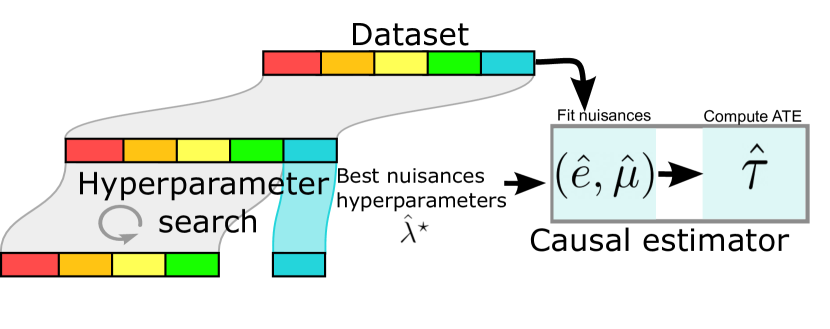
Figure 11: Hyper-parameter search procedure.

We followed a two-step procedure to train the nuisance models (eg. ($\hat{e},\hat{\mu}$) for the AIPW causal estimator), taking inspiration from the computationally cheap procedure from [13, section 3.3]. First, for each nuisance model, we fit a random parameter search with 5-fold cross validation and 10 iterations on the full dataset. Each iteration fit a model with a random combination of parameters in a predefined grid, then evaluate the performance by cross-validation. The best hyper-parameters $\hat{\lambda}^{\star}$ are selected as the ones reaching the minimal score across all iterations. Then, we feed this parameters to the causal estimator. The single robust estimators (matching, IPW and TLearner) refit the corresponding estimator only once on the full dataset, then estimate the ATE. The doubly-robust estimators use a cross-fitting procedure (K=5) to fit the nuisances then estimate the ATE. Figure 11 illustrates the procedure and Table 7 details the hyper-parameters grid for the random search.

	estimator	nuisance	Grid
Estimator type
Linear	LogisticRegression	treatment	{’C’: logspace(-3, 2, 10)}
Linear	Ridge	outcome	{’alpha’: logspace(-3, 2, 10)}
Forest	RandomForestClassifier	treatment	{’n_estimators’: [’10’, ’100’, ’200’], ’max_depth’: [’3’, ’10’, ’50’]}
Forest	RandomForestRegressor	outcome	{’n_estimators’: [’10’, ’100’, ’200’], ’max_depth’: [’3’, ’10’, ’50’]}

Table 7: Hyper-parameter grid used during random search optimization.

Appendix F Computing resources

The whole project was run on a laptop running Ubuntu 22.04.2 LTS with the following hardware: CPU 12th Gen Intel(R) Core(TM) i7-1270P with 16 threads and 15 GB of RAM.

Appendix G Selection flowchart

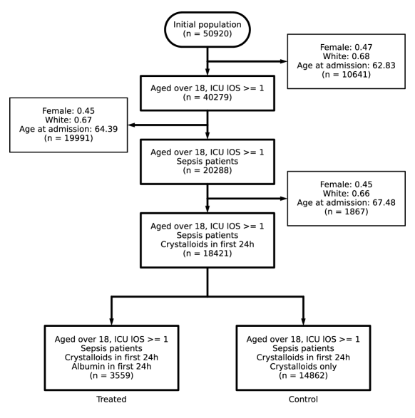
Figure 12: Selection flowchart on MIMIC-IV for the emulated trial.

Appendix H Complete description of the confounders for the main analysis

	Missing	Overall	Cristalloids only	Cristalloids + Albumin	P-Value
n		18421	14862	3559
Glycopeptide, n (%)		9492 (51.5)	7650 (51.5)	1842 (51.8)
Beta-lactams, n (%)		5761 (31.3)	5271 (35.5)	490 (13.8)
Carbapenems, n (%)		727 (3.9)	636 (4.3)	91 (2.6)
Aminoglycosides, n (%)		314 (1.7)	290 (2.0)	24 (0.7)
suspected_infection_blood, n (%)		170 (0.9)	149 (1.0)	21 (0.6)
RRT, n (%)		229 (1.2)	205 (1.4)	24 (0.7)
ventilation, n (%)		16376 (88.9)	12931 (87.0)	3445 (96.8)
vasopressors, n (%)		9058 (49.2)	6204 (41.7)	2854 (80.2)
Female, n (%)		7653 (41.5)	6322 (42.5)	1331 (37.4)
White, n (%)		12366 (67.1)	9808 (66.0)	2558 (71.9)
Emergency admission, n (%)		9605 (52.1)	8512 (57.3)	1093 (30.7)
Insurance, Medicare, n (%)		9727 (52.8)	7958 (53.5)	1769 (49.7)
myocardial_infarct, n (%)		3135 (17.0)	2492 (16.8)	643 (18.1)
malignant_cancer, n (%)		2465 (13.4)	2128 (14.3)	337 (9.5)
diabetes_with_cc, n (%)		1633 (8.9)	1362 (9.2)	271 (7.6)
diabetes_without_cc, n (%)		4369 (23.7)	3532 (23.8)	837 (23.5)
metastatic_solid_tumor, n (%)		1127 (6.1)	1016 (6.8)	111 (3.1)
severe_liver_disease, n (%)		1289 (7.0)	880 (5.9)	409 (11.5)
renal_disease, n (%)		3765 (20.4)	3159 (21.3)	606 (17.0)
aki_stage_0.0, n (%)		7368 (40.0)	6284 (42.3)	1084 (30.5)
aki_stage_1.0, n (%)		4019 (21.8)	3222 (21.7)	797 (22.4)
aki_stage_2.0, n (%)		6087 (33.0)	4605 (31.0)	1482 (41.6)
aki_stage_3.0, n (%)		947 (5.1)	751 (5.1)	196 (5.5)
SOFA, mean (SD)	0	6.0 (3.5)	5.7 (3.4)	6.9 (3.6)	<0.001
SAPSII, mean (SD)	0	40.3 (14.1)	39.8 (14.1)	42.8 (13.6)	<0.001
Weight, mean (SD)	97	83.3 (23.7)	82.5 (24.2)	86.4 (21.2)	<0.001
temperature, mean (SD)	966	36.9 (0.6)	36.9 (0.6)	36.8 (0.6)	<0.001
mbp, mean (SD)	0	75.6 (10.2)	76.3 (10.7)	72.4 (7.2)	<0.001
resp_rate, mean (SD)	9	19.3 (4.3)	19.6 (4.4)	18.0 (3.8)	<0.001
heart_rate, mean (SD)	0	86.2 (16.3)	86.2 (16.8)	86.5 (14.3)	0.197
spo2, mean (SD)	4	97.4 (2.2)	97.3 (2.3)	98.0 (2.1)	<0.001
lactate, mean (SD)	4616	3.0 (2.5)	2.8 (2.4)	3.7 (2.6)	<0.001
urineoutput, mean (SD)	301	24.0 (52.7)	24.7 (58.2)	21.1 (16.6)	<0.001
admission_age, mean (SD)	0	66.3 (16.2)	66.1 (16.8)	67.3 (13.1)	<0.001
delta mortality to inclusion, mean (SD)	11121	316.9 (640.2)	309.6 (628.8)	365.0 (708.9)	0.022
delta intervention to inclusion, mean (SD)	14862	0.3 (0.2)	nan (nan)	0.3 (0.2)	nan
delta inclusion to intime, mean (SD)	0	0.1 (0.2)	0.1 (0.2)	0.1 (0.1)	0.041
delta ICU intime to hospital admission, mean (SD)	0	1.1 (3.7)	1.0 (3.7)	1.6 (3.4)	<0.001
los_hospital, mean (SD)	0	12.6 (12.5)	12.6 (12.5)	12.9 (12.4)	0.189
los_icu, mean (SD)	0	5.5 (6.7)	5.5 (6.5)	5.5 (7.2)	0.605

Table 8: Characteristics of the trial population measured on the first 24 hours of ICU stay.
Risk scores (AKI, SOFA, SAPSII) and lactates have been summarized as the maximum value during the 24 hour period for each stay. Total cumulative urine output has been computed. Other variables have been aggregated by taking mean during the 24 hour period.

Appendix I Complete results for the main analysis

Compared to figure 7, we also report in figure 13 the estimates for Causal forest estimators and other choices of feature aggregation (first and last).

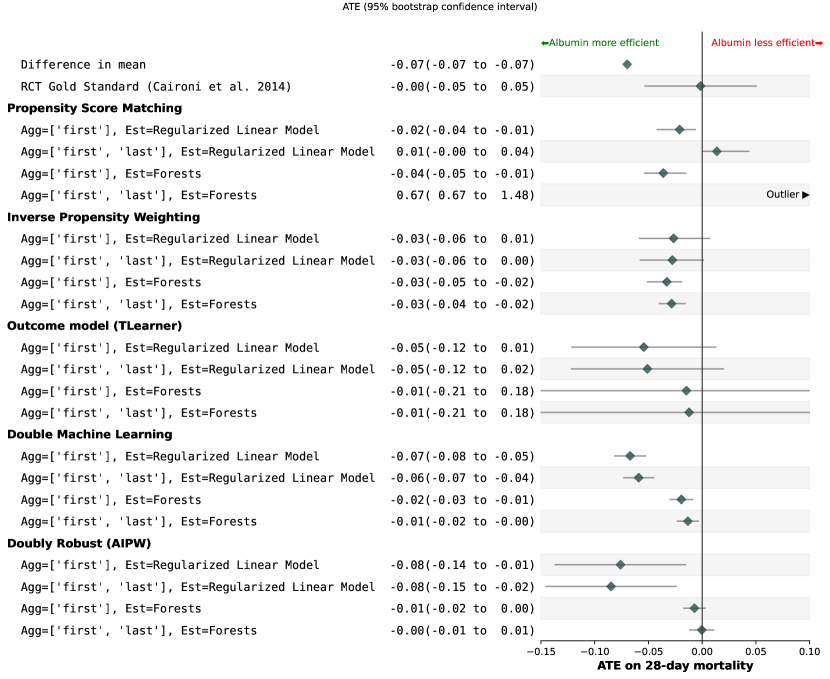
Figure 13: Full sensitivity analysis: The estimators with forest nuisances point to no effect for almost every causal estimator consistently with the RCT gold standard. Only matching with forest yields an unconvincingly high estimate. Linear nuisance used with doubly robust methods suggest a reduced mortality risk for albumin. The choices of aggregation only marginally modify the results expect for propensity score matching. The green diamonds depict the mean effect and the bar are the 95% confidence intervals obtained by 50 bootstrap repetitions.

Appendix J Complete results for the Immortal time bias

Compared to figure 3, we also report in figure 14 the estimates for Double Machine Learning, Inverse Propensity Weighting for both Random Forest and Ridge Regression. Feature aggregation was concatenation of first and last for all estimates.

Figure 14: Sensitivity analysis for immortal time bias: Every choice of estimates show an improvement of the albumin treatment when increasing the observation period, thus increasing the blank period between inclusion and administration of albumin. Aggregation was concatenation of first and last features. The green diamonds depict the mean effect and the bar are the 95% confidence intervals obtained by 50 bootstrap repetitions.

Appendix K Vibration analysis for aggregation

We conducted a dedicated vibration analysis on the different choices of features aggregation, studying the impact on the estimated ATE. We also studied if some choices of aggregation led to substantially poorer overlap.

We assessed overlap with two different methods. As recommended by [7], we did a graphical assessment by plotting the distribution of the estimated. The treatment model hyper-parameters were chosen by random search, then predicted propensity scores were obtained by refitting this estimator with cross-fitting on the full dataset.

As shown in Figure 15, we did not find substantial differences between methods when plotting graphically the distribution of the estimated propensity score.

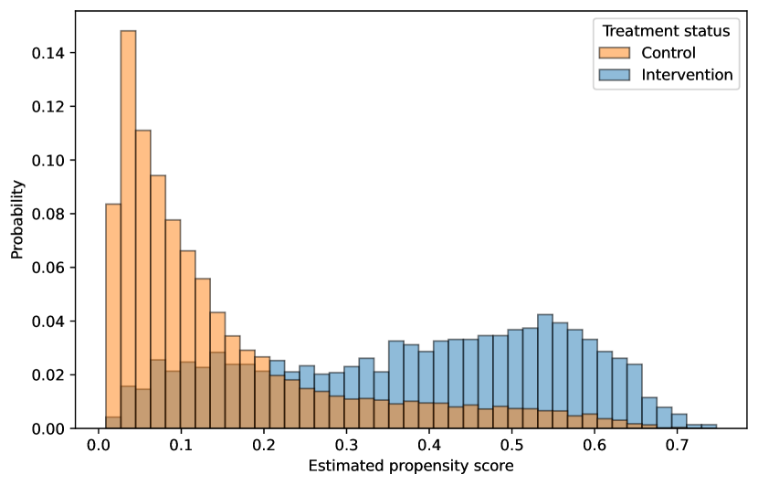
(a)

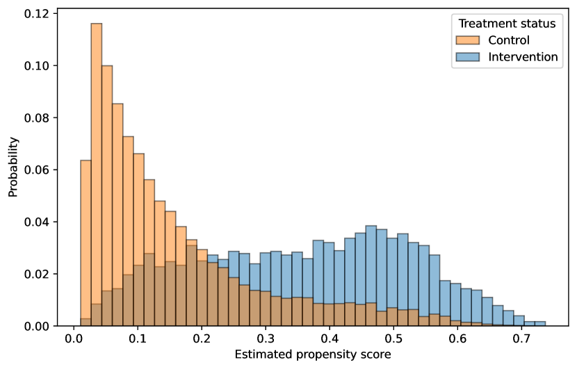
(b)

Figure 15: Different choices of aggregation yield qualitatively close distributions of the propensity score: Figure 15(a))a) shows a concatenation of first, last and median measures whereas Figure 15(b))b) shows an aggregation by taking the first measure only. The underlying treatment effect estimator is a random forest.

We also used normalized total variation (NTV) as a summary statistic of the estimated propensity score to measure the distance between treated and control population [26]. This statistic varies between 0 – perfect overlap – and 1 – no overlap at all. Fig 16 shows no marked differences in overlap as measured by NTV between aggregation choices, comforting us in our expert-driven choice of the aggregation: a concatenation of first and last feature observed before inclusion time.

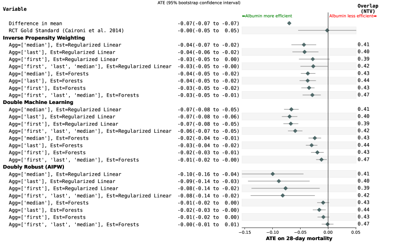
Figure 16: Vibration analysis dedicated to the aggregation choices. The choices of aggregation only marginally modify the results. When assessed with Normalized Total Variation, the overlap assumption is respected for all our choices of aggregation. The green diamonds depict the mean effect and the bar are the 95% confidence intervals obtained by 50 bootstrap repetitions.

Appendix L Details on treatment heterogeneity analysis

L.1 Detailed estimation procedure

The estimation of heterogeneous effect based on Double Machine Learning adds another step after the computation, regressing the residuals of the outcome nuisance $\tilde{Y}-\mu(X)$ against the residuals of the treatment nuisance $\tilde{A}=A-e(X)$ with the heterogeneity features $X_{CATE}$. Noting the final CATE model $\theta$, Double ML solves:

$$\operatorname*{arg\,min}_{\theta}\mathbb{E}_{n}\big{[}(\tilde{Y}-\theta(X_{CATE})\cdot\tilde{A})^{2}\big{]}$$

Where $\tilde{Y}=Y-\hat{\mu}(X,A)$ and $\tilde{A}=A-\hat{e}(X)$

To avoid the over-fitting of this last regression model, we split the dataset of the main analysis into a train set (size=0.8) where the causal estimator and the final model are learned, and a test set (size=0.2) on which we report the predicted Conditional Average Treatment Effects.

L.2 Known heterogeneity of treatment for the emulated trial

[15] observed statistical differences in the post-hoc subgroup analysis between patient with and without septic shock at inclusion. They found increasing treatment effect measured as relative risk for patients with septic shock (RR=0.87; 95% CI, 0.77 to 0.99 vs 1.13;95% CI, 0.92 to 1.39).

[51] conducted a post-hoc subgroup analysis of patients with or without brain injury –defined as Glasgow Coma Scale between 3 to 8–. The initial population was patients with traumatic brain injury (defined as history or evidence on A CT scan of head trauma, and a GCS score <= 13). They found higher mortality rate at 24 months in the albumin group for patients with severe head injuries.

[137] conducted a subgroup analysis on age (<60 vs >60), septic shock and sex. They conclude for increasing treatment effect measured as Restricted Mean Survival Time for Sepsis vs septic shock (3.47 vs. 2.58), for age >=60 (3.75 vs 2.44), for Male (3.4 vs 2.69). None of these differences were statistically significant.

L.3 Vibration analysis

The choice of the final model for the CATE estimation should also be informed by statistical and clinical rationals. Figure 17 shows the distribution of the individual effects of a final random forest estimator, yielding CATE estimates that are not consistent with the main ATE analysis. Figure 18 shows that the choice of this final model imposes a inductive bias on the form of the heterogeneity and different sources of noise depending of the nature of the model. A random forest is more noisy than a linear model. Figure 18 shows the difference of modelization on the subpopulation of non white male patients without septic shock. One see that the downside linear trend is reflected by the forest only for patients aged between 55 and 80.

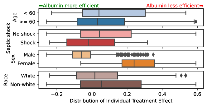
Figure 17: Distribution of Conditional Average Treatment effects on sex, age, race and pre-treatment septic shock estimated with a final forest estimator. The CATE are positive for each subgroups, which is not consistent with the null treatment effect obtained in the main analysis. The boxes contain between the 25th and 75th percentiles of the CATE distributions with the median indicated by a vertical line. The whiskers extends to 1.5 the inter-quartile range of the distribution.

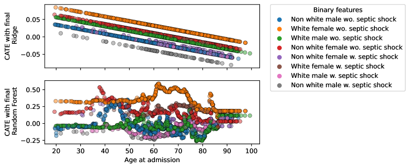
Figure 18: Distribution of Conditional Average Treatment effects on sex, age, race and pre-treatment septic shock plotted for different ages. On the top the final estimator is a linear model; on the bottom, it is a random forest. The forest-based CATE displays more noisy trends than the linear-based CATE. This suggest that the flexibility of the random forest might be underfitting the data.

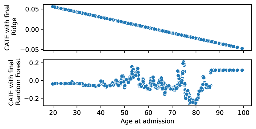
Figure 19: Figure 18 on the subpopulation of white male patients without septic shock. Contrary to the ridge regression (on top) inducing a nicely interpretable trend, using random forests as the final estimator failed to recover CATE on ages: the predicted estimates do not exhibit any trend and display inconsistently large effect sizes, suggesting data underfitting.

References

- [1] Alberto Abadie and Guido W Imbens “On the failure of the bootstrap for matching estimators” In Econometrica 76.6 Wiley Online Library, 2008, pp. 1537–1557
- [2] Hammaad Adam et al. “Write It Like You See It: Detectable Differences in Clinical Notes by Race Lead to Differential Model Recommendations” In AAAI/ACM Conference on AI, Ethics, and Society, 2022
- [3] Mohammad Adibuzzaman et al. “Methods for quantifying efficacy-effectiveness gap of randomized controlled trials: examples in ards” In Critical Care Medicine 47.1 LWW, 2019, pp. 143
- [4] Ravi Aggarwal et al. “Diagnostic accuracy of deep learning in medical imaging: a systematic review and meta-analysis” In NPJ digital medicine 4.1 Nature Publishing Group UK London, 2021, pp. 65
- [5] Djillali Annane et al. “Effects of fluid resuscitation with colloids vs crystalloids on mortality in critically ill patients presenting with hypovolemic shock: the CRISTAL randomized trial” In Jama 310.17 American Medical Association, 2013, pp. 1809–1817
- [6] John Attia, Elizabeth Holliday and Christopher Oldmeadow “A proposal for capturing interaction and effect modification using DAGs” In International Journal of Epidemiology 51.4 Oxford University Press, 2022, pp. 1047–1053
- [7] Peter C Austin and Elizabeth A Stuart “Moving towards best practice when using inverse probability of treatment weighting (IPTW) using the propensity score to estimate causal treatment effects in observational studies” In Statistics in medicine 34.28 Wiley Online Library, 2015, pp. 3661–3679
- [8] Amelia J Averitt, Chunhua Weng, Patrick Ryan and Adler Perotte “Translating evidence into practice: eligibility criteria fail to eliminate clinically significant differences between real-world and study populations” In NPJ digital medicine 3.1 Nature Publishing Group UK London, 2020, pp. 67
- [9] Nunan D. Bankhead C “Attrition bias, Catalogue of Bias Collaboration.” Catalogue of Bias, 2017 URL: https://catalogofbias.org/biases/attrition-bias/
- [10] Keith Battocchi et al. “EconML: A Python Package for ML-Based Heterogeneous Treatment Effects Estimation” Version 0.14.0, 2019 URL: %5Curl%7Bhttps://github.com/py-why/EconML%7D
- [11] Brett K Beaulieu-Jones et al. “Machine learning for patient risk stratification: standing on, or looking over, the shoulders of clinicians?” In NPJ digital medicine 4.1 Nature Publishing Group UK London, 2021, pp. 62
- [12] Alexandre Belloni, Victor Chernozhukov and Christian Hansen “High-dimensional methods and inference on structural and treatment effects” In Journal of Economic Perspectives 28.2 American Economic Association 2014 Broadway, Suite 305, Nashville, TN 37203-2418, 2014, pp. 29–50
- [13] Xavier Bouthillier et al. “Accounting for variance in machine learning benchmarks” In Proceedings of Machine Learning and Systems 3, 2021, pp. 747–769
- [14] Nate Breznau et al. “Observing many researchers using the same data and hypothesis reveals a hidden universe of uncertainty” In Proceedings of the National Academy of Sciences 119.44 National Acad Sciences, 2022, pp. e2203150119
- [15] Pietro Caironi et al. “Albumin replacement in patients with severe sepsis or septic shock” In New England Journal of Medicine 370.15 Mass Medical Soc, 2014, pp. 1412–1421
- [16] Canadian Medical Association “Appropriateness in Health Care” In Canadian Medical Association Policy, 2015
- [17] Anthony Leo Celi et al. “An Open Benchmark for Causal Inference Using the MIMIC-III Dataset”, 2016
- [18] Victor Chernozhukov et al. “Double/debiased machine learning for treatment and structural parameters” Oxford University Press Oxford, UK, 2018
- [19] Eric E Chinaeke et al. “The impact of statin use prior to intensive care unit admission on critically ill patients with sepsis” In Pharmacotherapy: The Journal of Human Pharmacology and Drug Therapy 41.2 Wiley Online Library, 2021, pp. 162–171
- [20] Bénédicte Colnet, Julie Josse, Gaël Varoquaux and Erwan Scornet “Risk ratio, odds ratio, risk difference… Which causal measure is easier to generalize?” In arXiv preprint arXiv:2303.16008, 2023
- [21] Keith A Corl et al. “The Restrictive Intravenous Fluid Trial in Severe Sepsis and Septic Shock (RIFTS): a Randomized Pilot Study” In Critical care medicine 47.7 NIH Public Access, 2019, pp. 951
- [22] Alexander D’Amour et al. “Overlap in observational studies with high-dimensional covariates” In Journal of Econometrics 221.2 Elsevier, 2021, pp. 644–654
- [23] Alex J DeGrave, Joseph D Janizek and Su-In Lee “AI for radiographic COVID-19 detection selects shortcuts over signal” In Nature Machine Intelligence 3.7 Nature Publishing Group UK London, 2021, pp. 610–619
- [24] Rishi J Desai et al. “Broadening the reach of the FDA Sentinel System: a roadmap for integrating electronic health record data in a causal analysis framework” In NPJ digital medicine 4.1 Nature Publishing Group UK London, 2021, pp. 170
- [25] Vincent Dorie et al. “Automated versus Do-It-Yourself Methods for Causal Inference” In Statistical Science 34.1 JSTOR, 2019, pp. 43–68
- [26] Matthieu Doutreligne and Gaël Varoquaux “How to select predictive models for causal inference?” In arXiv preprint arXiv:2302.00370, 2023
- [27] Daniel E Ehrmann et al. “Making machine learning matter to clinicians: model actionability in medical decision-making” In NPJ Digital Medicine 6.1 Nature Publishing Group UK London, 2023, pp. 7
- [28] Andre Esteva et al. “Deep learning-enabled medical computer vision” In NPJ digital medicine 4.1 Nature Publishing Group UK London, 2021, pp. 5
- [29] FDA “Statistical Principles for Clinical Trials: Addendum: Estimands and Sensitivity Analysis in Clinical Trials”, 2021
- [30] Mengling Feng et al. “Transthoracic echocardiography and mortality in sepsis: analysis of the MIMIC-III database” In Intensive care medicine 44 Springer, 2018, pp. 884–892
- [31] Dylan J Foster and Vasilis Syrgkanis “Orthogonal statistical learning” In arXiv preprint arXiv:1901.09036, 2019
- [32] Edouard L Fu et al. “Timing of dialysis initiation to reduce mortality and cardiovascular events in advanced chronic kidney disease: nationwide cohort study” In bmj 375 British Medical Journal Publishing Group, 2021
- [33] Md Osman Gani et al. “Structural causal model with expert augmented knowledge to estimate the effect of oxygen therapy on mortality in the icu” In Artificial Intelligence in Medicine 137 Elsevier, 2023, pp. 102493
- [34] Robert Geirhos et al. “Shortcut learning in deep neural networks” In Nature Machine Intelligence 2.11 Nature Publishing Group UK London, 2020, pp. 665–673
- [35] Marzyeh Ghassemi et al. “A review of challenges and opportunities in machine learning for health” In AMIA Summits on Translational Science Proceedings 2020 American Medical Informatics Association, 2020, pp. 191
- [36] Judy Wawira Gichoya et al. “AI recognition of patient race in medical imaging: a modelling study” In The Lancet Digital Health 4.6 Elsevier, 2022, pp. e406–e414
- [37] Google “Tensorflow Responsible AI”, 2023 URL: https://www.tensorflow.org/responsible_ai
- [38] Sander Greenland, Judea Pearl and James M Robins “Causal diagrams for epidemiologic research” In Epidemiology JSTOR, 1999, pp. 37–48
- [39] Miguel A Hernan “Methods of public health research–strengthening causal inference from observational data” In New England Journal of Medicine 385.15 Mass Medical Soc, 2021, pp. 1345–1348
- [40] Miguel A Hernan, John Hsu and Brian Healy “A second chance to get causal inference right: a classification of data science tasks” In Chance 32.1 Taylor & Francis, 2019, pp. 42–49
- [41] Miguel A Hernan et al. “Specifying a target trial prevents immortal time bias and other self-inflicted injuries in observational analyses” In Journal of clinical epidemiology 79 Elsevier, 2016, pp. 70–75
- [42] Miguel A Hernàn and James M Robins “Causal inference: What If.”, 2020
- [43] Miguel A. Hernán and James M. Robins “Using Big Data to Emulate a Target Trial When a Randomized Trial Is Not Available” In American Journal of Epidemiology 183.8, 2016
- [44] Gonzalo Hernandez et al. “Effect of postextubation high-flow nasal cannula vs noninvasive ventilation on reintubation and postextubation respiratory failure in high-risk patients: a randomized clinical trial” In Jama 316.15 American Medical Association, 2016, pp. 1565–1574
- [45] An Thi Nhat Ho, Setu Patolia and Christophe Guervilly “Neuromuscular blockade in acute respiratory distress syndrome: a systematic review and meta-analysis of randomized controlled trials” In Journal of intensive care 8 Springer, 2020, pp. 1–11
- [46] Robin Hofmann et al. “Oxygen therapy in suspected acute myocardial infarction” In New England Journal of Medicine 377.13 Mass Medical Soc, 2017, pp. 1240–1249
- [47] Steven Horng et al. “Creating an automated trigger for sepsis clinical decision support at emergency department triage using machine learning” In PloS one 12.4 Public Library of Science San Francisco, CA USA, 2017, pp. e0174708
- [48] Douglas J Hsu et al. “The association between indwelling arterial catheters and mortality in hemodynamically stable patients with respiratory failure: a propensity score analysis” In Chest 148.6 Elsevier, 2015, pp. 1470–1476
- [49] Guido W Imbens and Jeffrey M Wooldridge “Recent developments in the econometrics of program evaluation” In Journal of economic literature 47.1 American Economic Association, 2009, pp. 5–86
- [50] Guido W. Imbens “Nonparametric Estimation of Average Treatment Effects Under Exogeneity: A Review” In The Review of Economics and Statistics 86.1, 2004, pp. 4–29 DOI: 10.1162/003465304323023651
- [51] SAFE Study Investigators “Saline or albumin for fluid resuscitation in patients with traumatic brain injury” In New England Journal of Medicine 357.9 Mass Medical Soc, 2007, pp. 874–884
- [52] John PA Ioannidis “Why most published research findings are false” In PLoS medicine 2.8 Public Library of Science, 2005, pp. e124
- [53] Andrew Jesson, Sören Mindermann, Uri Shalit and Yarin Gal “Identifying causal-effect inference failure with uncertainty-aware models” In Advances in Neural Information Processing Systems 33, 2020, pp. 11637–11649
- [54] Lavender Yao Jiang et al. “Health system-scale language models are all-purpose prediction engines” In Nature Nature Publishing Group UK London, 2023, pp. 1–6
- [55] Alistair Johnson et al. “Mimic-iv” In PhysioNet. Available online at: https://physionet. org/content/mimiciv/1.0/(accessed August 23, 2021), 2020
- [56] Tessa Kennedy-Martin et al. “A literature review on the representativeness of randomized controlled trial samples and implications for the external validity of trial results” In Trials 16 Springer, 2015, pp. 1–14
- [57] David M Kent, Ewout Steyerberg and David Klaveren “Personalized evidence based medicine: predictive approaches to heterogeneous treatment effects” In Bmj 363 British Medical Journal Publishing Group, 2018
- [58] Tak Kyu Oh et al. “Preadmission statin use and 90-day mortality in the critically ill: a retrospective association study” In Anesthesiology 131.2, 2019, pp. 315–327
- [59] H. Lee and D. Nunan “Immortal time bias, Catalogue of Bias Collaboration.” Catalogue of Bias, 2020 URL: https://catalogofbias.org/biases/immortaltimebias/
- [60] MG Lee et al. “Preadmission statin use improves the outcome of less severe sepsis patients-a population-based propensity score matched cohort study” In BJA: British Journal of Anaesthesia 119.4 Oxford University Press, 2017, pp. 645–654
- [61] Binghu Li et al. “Resuscitation fluids in septic shock: a network meta-analysis of randomized controlled trials” In Shock 53.6 LWW, 2020, pp. 679–685
- [62] Yikuan Li et al. “BEHRT: transformer for electronic health records” In Scientific reports 10.1 Springer, 2020, pp. 1–12
- [63] Taotao Liu, Qinyu Zhao and Bin Du “Effects of high-flow oxygen therapy on patients with hypoxemia after extubation and predictors of reintubation: a retrospective study based on the MIMIC-IV database” In BMC Pulmonary Medicine 21.1 BioMed Central, 2021, pp. 1–15
- [64] Xiaoxuan Liu et al. “A comparison of deep learning performance against health-care professionals in detecting diseases from medical imaging: a systematic review and meta-analysis” In The lancet digital health 1.6 Elsevier, 2019, pp. e271–e297
- [65] Min Lu, Saad Sadiq, Daniel J Feaster and Hemant Ishwaran “Estimating individual treatment effect in observational data using random forest methods” In Journal of Computational and Graphical Statistics 27.1 Taylor & Francis, 2018, pp. 209–219
- [66] Diane Mackle et al. “Conservative oxygen therapy during mechanical ventilation in the ICU.” In The New England journal of medicine 382.11, 2019, pp. 989–998
- [67] Manu LNG Malbrain et al. “Fluid overload, de-resuscitation, and outcomes in critically ill or injured patients: a systematic review with suggestions for clinical practice” In Anaesthesiology intensive therapy 46.5, 2014, pp. 361–380
- [68] Jess Mandel and Paul M Palevsky “Treatment of severe hypovolemia or hypovolemic shock in adults” In UpToDate, 2023
- [69] Tine Sylvest Meyhoff et al. “Lower vs higher fluid volumes during initial management of sepsis: a systematic review with meta-analysis and trial sequential analysis” In Chest 157.6 Elsevier, 2020, pp. 1478–1496
- [70] Microsoft “Responsible AI toolbox”, 2023 URL: https://responsibleaitoolbox.ai
- [71] Nandita Mitra, Jason Roy and Dylan Small “The Future of Causal Inference” In American Journal of Epidemiology 191.10 Oxford University Press, 2022, pp. 1671–1676
- [72] Raha Moraffah et al. “Causal inference for time series analysis: Problems, methods and evaluation” In Knowledge and Information Systems 63 Springer, 2021, pp. 3041–3085
- [73] Laveena Munshi et al. “Prone position for acute respiratory distress syndrome. A systematic review and meta-analysis” In Annals of the American Thoracic Society 14.Supplement 4 American Thoracic Society, 2017, pp. S280–S288
- [74] Lung National Heart and Blood Institute ARDS Clinical Trials Network “Higher versus lower positive end-expiratory pressures in patients with the acute respiratory distress syndrome” In New England Journal of Medicine 351.4 Mass Medical Soc, 2004, pp. 327–336
- [75] Lung National Heart and Blood Institute ARDS Clinical Trials Network “Rosuvastatin for sepsis-associated acute respiratory distress syndrome” In New England Journal of Medicine 370.23 Mass Medical Soc, 2014, pp. 2191–2200
- [76] Eric Neumayer and Thomas Plümper “Robustness tests for quantitative research” Cambridge University Press, 2017
- [77] Xinkun Nie and Stefan Wager “Quasi-oracle estimation of heterogeneous treatment effects” In Biometrika 108.2 Oxford University Press, 2021, pp. 299–319
- [78] OHDSI “The Book of OHDSI: Observational Health Data Sciences and Informatics” OHDSI, 2021 URL: https://ohdsi.github.io/TheBookOfOhdsi/
- [79] J. Oke, T. Fanshawe and D. Nunan “Lead time bias, Catalogue of Bias Collaboration.” Catalogue of Bias, 2021 URL: https://catalogofbias.org/biases/lead-time-bias/
- [80] Rakshit Panwar et al. “Conservative versus liberal oxygenation targets for mechanically ventilated patients. A pilot multicenter randomized controlled trial” In American journal of respiratory and critical care medicine 193.1 American Thoracic Society, 2016, pp. 43–51
- [81] Laurent Papazian et al. “Neuromuscular blockers in early acute respiratory distress syndrome” In New England Journal of Medicine 363.12 Mass Medical Soc, 2010, pp. 1107–1116
- [82] Chirag J Patel, Belinda Burford and John PA Ioannidis “Assessment of vibration of effects due to model specification can demonstrate the instability of observational associations” In Journal of clinical epidemiology 68.9 Elsevier, 2015, pp. 1046–1058
- [83] Judea Pearl and Dana Mackenzie “The book of why: the new science of cause and effect” Basic books, 2018
- [84] Fabian Pedregosa et al. “Scikit-learn: Machine learning in Python” In the Journal of machine Learning research 12 JMLR. org, 2011, pp. 2825–2830
- [85] Drago Plecko and Elias Bareinboim “Causal fairness analysis” In arXiv preprint arXiv:2207.11385, 2022
- [86] Mattia Prosperi et al. “Causal inference and counterfactual prediction in machine learning for actionable healthcare” In Nature Machine Intelligence 2.7 Nature Publishing Group UK London, 2020, pp. 369–375
- [87] PwC “Responsible AI Toolkit”, 2023 URL: https://www.pwc.com/gx/en/issues/data-and-analytics/artificial-intelligence/what-is-responsible-ai.html
- [88] Alvin Rajkomar et al. “Ensuring fairness in machine learning to advance health equity” In Annals of internal medicine 169.12 American College of Physicians, 2018, pp. 866–872
- [89] Alvin Rajkomar et al. “Scalable and accurate deep learning with electronic health records” In NPJ digital medicine 1.1 Nature Publishing Group UK London, 2018, pp. 18
- [90] Alexandros Rekkas et al. “A standardized framework for risk-based assessment of treatment effect heterogeneity in observational healthcare databases” In npj Digital Medicine 6.1 Nature Publishing Group UK London, 2023, pp. 58
- [91] W Scott Richardson, Mark C Wilson, Jim Nishikawa and Robert S Hayward “The well-built clinical question: a key to evidence-based decisions” In Acp j club 123.3, 1995, pp. A12–A13
- [92] Jonathan G Richens, Ciarán M Lee and Saurabh Johri “Improving the accuracy of medical diagnosis with causal machine learning” In Nature communications 11.1 Nature Publishing Group UK London, 2020, pp. 3923
- [93] John J Riva et al. “What is your research question? An introduction to the PICOT format for clinicians” In The Journal of the Canadian Chiropractic Association 56.3 The Canadian Chiropractic Association, 2012, pp. 167
- [94] Sarah E Robertson, Andrew Leith, Christopher H Schmid and Issa J Dahabreh “Assessing heterogeneity of treatment effects in observational studies” In American Journal of Epidemiology 190.6 Oxford University Press, 2021, pp. 1088–1100
- [95] James M Robins and Sander Greenland “The role of model selection in causal inference from nonexperimental data” In American Journal of Epidemiology 123.3 Oxford University Press, 1986, pp. 392–402
- [96] James M Robins, Andrea Rotnitzky and Lue Ping Zhao “Estimation of regression coefficients when some regressors are not always observed” In Journal of the American statistical Association 89.427 Taylor & Francis, 1994, pp. 846–866
- [97] Peter M Robinson “Root-N-consistent semiparametric regression” In Econometrica: Journal of the Econometric Society JSTOR, 1988, pp. 931–954
- [98] Eliane Röösli, Selen Bozkurt and Tina Hernandez-Boussard “Peeking into a black box, the fairness and generalizability of a MIMIC-III benchmarking model” In Scientific Data 9.1 Nature Publishing Group UK London, 2022, pp. 24
- [99] Paul R Rosenbaum and Donald B Rubin “The central role of the propensity score in observational studies for causal effects” In Biometrika 70, 1983, pp. 41–55
- [100] Peter M Rothwell “Factors that can affect the external validity of randomised controlled trials” In PLoS clinical trials 1.1 Public Library of Science San Francisco, USA, 2006, pp. e9
- [101] Donald B Rubin “Causal inference using potential outcomes: Design, modeling, decisions” In Journal of the American Statistical Association 100.469 Taylor & Francis, 2005, pp. 322–331
- [102] SAFE Study Investigators “Impact of albumin compared to saline on organ function and mortality of patients with severe sepsis” In Intensive care medicine 37 Springer, 2011, pp. 86–96
- [103] Sebastian Schneeweiss “Sensitivity analysis and external adjustment for unmeasured confounders in epidemiologic database studies of therapeutics” In Pharmacoepidemiology and drug safety 15.5 Wiley Online Library, 2006, pp. 291–303
- [104] Sebastian Schneeweiss and Elisabetta Patorno “Conducting real-world evidence studies on the clinical outcomes of diabetes treatments” In Endocrine Reviews 42.5 Oxford University Press US, 2021, pp. 658–690
- [105] Bernhard Schölkopf et al. “Toward causal representation learning” In Proceedings of the IEEE 109.5 IEEE, 2021, pp. 612–634
- [106] Megan S Schuler and Sherri Rose “Targeted maximum likelihood estimation for causal inference in observational studies” In American journal of epidemiology 185.1 Oxford University Press, 2017, pp. 65–73
- [107] Laleh Seyyed-Kalantari et al. “Underdiagnosis bias of artificial intelligence algorithms applied to chest radiographs in under-served patient populations” In Nature medicine 27.12 Nature Publishing Group US New York, 2021, pp. 2176–2182
- [108] Zach Shahn et al. “Fluid-limiting treatment strategies among sepsis patients in the ICU: a retrospective causal analysis” In Critical Care 24.1 BioMed Central, 2020, pp. 1–9
- [109] Uri Shalit and David Sontag “Causal Inference for Observational studies: Tutorial” In ICML, 2016 URL: https://docplayer.net/64797211-Causal-inference-for-observational-studies.html
- [110] Amit Sharma “Tutorial on causal inference and counterfactual reasoning”, 2018 URL: https://causalinference.gitlab.io/kdd-tutorial/
- [111] Harvineet Singh, Vishwali Mhasawade and Rumi Chunara “Generalizability challenges of mortality risk prediction models: A retrospective analysis on a multi-center database” In PLOS Digital Health 1.4 Public Library of Science San Francisco, CA USA, 2022, pp. e0000023
- [112] Ratender Kumar Singh et al. “The effects of atorvastatin on inflammatory responses and mortality in septic shock: a single-center, randomized controlled trial” In Indian Journal of Critical Care Medicine: Peer-reviewed, Official Publication of Indian Society of Critical Care Medicine 21.10 Indian Society of Critical Care Medicine, 2017, pp. 646
- [113] Jonathan M Snowden, Sherri Rose and Kathleen M Mortimer “Implementation of G-computation on a simulated data set: demonstration of a causal inference technique” In American journal of epidemiology 173.7 Oxford University Press, 2011, pp. 731–738
- [114] Oleg Sofrygin et al. “Targeted learning with daily EHR data” In Statistics in medicine 38.16 Wiley Online Library, 2019, pp. 3073–3090
- [115] François Stéphan et al. “High-flow nasal oxygen vs noninvasive positive airway pressure in hypoxemic patients after cardiothoracic surgery: a randomized clinical trial” In Jama 313.23 American Medical Association, 2015, pp. 2331–2339
- [116] Ralph AH Stewart et al. “High flow oxygen and risk of mortality in patients with a suspected acute coronary syndrome: pragmatic, cluster randomised, crossover trial” In bmj 372 British Medical Journal Publishing Group, 2021
- [117] Elizabeth A Stuart “Matching methods for causal inference: A review and a look forward” In Statistical science: a review journal of the Institute of Mathematical Statistics 25.1 NIH Public Access, 2010, pp. 1
- [118] Samy Suissa “Immortal time bias in pharmacoepidemiology” In American journal of epidemiology 167.4 Oxford University Press, 2008, pp. 492–499
- [119] Johannes Textor, Juliane Hardt and Sven Knüppel “DAGitty: a graphical tool for analyzing causal diagrams” In Epidemiology 22.5 LWW, 2011, pp. 745 URL: http://dagitty.net/
- [120] Lehana Thabane et al. “A tutorial on sensitivity analyses in clinical trials: the what, why, when and how” In BMC medical research methodology 13.1 BioMed Central, 2013, pp. 1–12
- [121] Justin Travers et al. “External validity of randomised controlled trials in asthma: to whom do the results of the trials apply?” In Thorax 62.3 BMJ Publishing Group Ltd, 2007, pp. 219–223
- [122] Chien-Hua Tseng et al. “Resuscitation fluid types in sepsis, surgical, and trauma patients: a systematic review and sequential network meta-analyses” In Critical Care 24.1 BioMed Central, 2020, pp. 1–12
- [123] Mark J Van der Laan, Eric C Polley and Alan E Hubbard “Super learner” In Statistical applications in genetics and molecular biology 6.1 De Gruyter, 2007
- [124] Tyler J VanderWeele “Principles of confounder selection” In European journal of epidemiology 34 Springer, 2019, pp. 211–219
- [125] Stefan Wager “Stats 361: Causal inference”, 2020
- [126] You-Dong Wan et al. “Effect of statin therapy on mortality from infection and sepsis: a meta-analysis of randomized and observational studies” In Critical care 18 Springer, 2014, pp. 1–13
- [127] Jun Wang et al. “Early Enteral Nutrition and Sepsis-Associated Acute Kidney Injury: A Propensity Score Matched Cohort Study Based on the MIMIC-III Database” In Yonsei Medical Journal 64.4, 2023, pp. 259–268
- [128] Shirley V Wang et al. “Emulation of randomized clinical trials with nonrandomized database analyses: results of 32 clinical trials” In JAMA 329.16 American Medical Association, 2023, pp. 1376–1385
- [129] Shirley V Wang, Sushama Kattinakere Sreedhara, Lily G Bessette and Sebastian Schneeweiss “Understanding variation in the results of real-world evidence studies that seem to address the same question” In Journal of Clinical Epidemiology 151 Elsevier, 2022, pp. 161–170
- [130] Nicole G Weiskopf et al. “Healthcare utilization is a collider: an introduction to collider bias in EHR data reuse” In Journal of the American Medical Informatics Association Oxford University Press, 2023, pp. ocad013
- [131] Thierry Wendling et al. “Comparing methods for estimation of heterogeneous treatment effects using observational data from health care databases” In Statistics in medicine 37.23 Wiley Online Library, 2018, pp. 3309–3324
- [132] Julia K Winkler et al. “Association between surgical skin markings in dermoscopic images and diagnostic performance of a deep learning convolutional neural network for melanoma recognition” In JAMA dermatology 155.10 American Medical Association, 2019, pp. 1135–1141
- [133] Jing-Yuan Xu et al. “Comparison of the effects of albumin and crystalloid on mortality in adult patients with severe sepsis and septic shock: a meta-analysis of randomized clinical trials” In Critical Care 18.6 BioMed Central, 2014, pp. 1–8
- [134] Ryo Yamamoto et al. “Hydrocortisone with fludrocortisone for septic shock: a systematic review and meta-analysis” In Acute medicine & surgery 7.1 Wiley Online Library, 2020, pp. e563
- [135] Christopher J Yarnell et al. “Oxygenation thresholds for invasive ventilation in hypoxemic respiratory failure: a target trial emulation in two cohorts” In Critical Care 27.1 BioMed Central, 2023, pp. 1–13
- [136] Jiaming Zeng et al. “Uncovering interpretable potential confounders in electronic medical records” In Nature Communications 13.1 Nature Publishing Group UK London, 2022, pp. 1014
- [137] Shiyu Zhou et al. “Early combination of albumin with crystalloids administration might be beneficial for the survival of septic patients: a retrospective analysis from MIMIC-IV database” In Annals of intensive care 11 Springer, 2021, pp. 1–10