Unsupervised Multiplex Graph Learning
with Complementary and Consistent Information

Abstract.

Unsupervised multiplex graph learning (UMGL) has been shown to achieve significant effectiveness for different downstream tasks by exploring both complementary information and consistent information among multiple graphs. However, previous methods usually overlook the issues in practical applications, i.e., the out-of-sample issue and the noise issue. To address the above issues, in this paper, we propose an effective and efficient UMGL method to explore both complementary and consistent information. To do this, our method employs multiple MLP encoders rather than graph convolutional network (GCN) to conduct representation learning with two constraints, i.e., preserving the local graph structure among nodes to handle the out-of-sample issue, and maximizing the correlation of multiple node representations to handle the noise issue. Comprehensive experiments demonstrate that our proposed method achieves superior effectiveness and efficiency over the comparison methods and effectively tackles those two issues. Code is available at https://github.com/LarryUESTC/CoCoMG.

1. Introduction

Multiplex graph is a type of data that consists of multiple graphs, where each graph represents a different type of relationship among nodes (Battiston et al., 2017; Gan et al., 2022; Liu et al., 2022). This kind of data is prevalent in various practical applications, such as social networks and biological networks (Zhang et al., 2019; Zhu et al., 2022a; Yuan et al., 2021; Li et al., 2021). Recently, there has been growing interest in unsupervised multiplex graph learning (UMGL) due to its ability to extract valuable information from multiple relationships among nodes without relying on label information (Park et al., 2020; Chu et al., 2019; Zhang et al., 2022; Wang et al., 2022b).

The success of existing UMGL methods lies in that they are able to explore both complementary information and consistent information among multiple graphs, so that UMGL can provide more comprehensive information than graph learning on the single graph (Chu et al., 2019; Zhou et al., 2020; Xie et al., 2023). The complementary information refers to different types of relationships that can supply each other and provide a more comprehensive understanding of the hidden patterns or structures in the data (Cen et al., 2019). For example, friendships and communication relationships provide complementary information to identify individuals belonging to the same social circle (Wang et al., 2022a). The consistent information means consistent relationships among nodes or structures across multiple graphs, which can help the model recognize the same category effectively. For example, the consistency of gene expression and protein-protein interactions is helpful to identify categories in biological networks (Zhu et al., 2022b; Li et al., 2021). Obviously, either complementary information or consistent information often plays an important role in UMGL.

Various methods have been proposed in the literature (Park et al., 2020; Wang et al., 2021; Jing et al., 2021; Zhu et al., 2022b) to explore and leverage either complementary information or consistent information. For instance, Jing et al. apply graph convolutional networks (GCN) (Kipf and Welling, 2016) to first obtain representations from each graph and then to fuse these representations by an attention mechanism (Vaswani et al., 2017), aiming at exploring complementary information among multiple graphs (Jing et al., 2021). However, its effectiveness is limited by the noisy information as it ignores the intrinsic correlation (i.e., consistent information) across different graphs. To address this limitation, recent researchers (Park et al., 2020; Wang et al., 2021; Zhu et al., 2022b; Jing et al., 2022a) have explored contrastive learning techniques (Oord et al., 2018) to simultaneously explore complementary and consistent information for UMGL. For example, to explore the consistent information, Park et al. conduct contrastive learning between node representations and graph representations (Park et al., 2020; Jing et al., 2021) and Zhu et al. conduct contrastive learning among node representations from different graphs (Zhu et al., 2022b). Thus, it is crucial to learn both complementary information and consistent information for conducting UMGL.

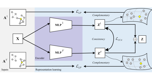
Figure 1. The flowchart of the proposed CoCoMG. Given the original node feature matrix $\mathbf{X}$, CoCoMG employs MLP encoders with two constraints ($\mathcal{L}_{LP}$ and $\mathcal{L}_{CCA}$) to generate representation $\mathbf{Z}^{v}$ ($v=1,...,V$). Specifically, the local preserve loss $\mathcal{L}_{LP}$ is designed to extract the complementary information of every graph and deal with the out-of-sample issue. The canonical correlation analysis (CCA) loss $\mathcal{L}_{CCA}$ is designed to extract the consistent information among all graphs and deal with the noise issue. Finally, the final representation $\mathbf{Z}$ is obtained for downstream tasks by averagely fusing all representations.

Despite the important advances, previous UMGL methods for simultaneously considering complementary and consistent information usually overlook some issues, such as the out-of-sample issue (Ma et al., 2018) and the noise issue (Zhao et al., 2017), resulting in a gap between the existing methods and their practical applications. On the one hand, previous UMGL methods (Park et al., 2020; Wang et al., 2021; Jing et al., 2021; Zhu et al., 2022b; Han et al., 2023) can not directly infer representations for unseen nodes because they do not directly generate a prediction model to predict unseen nodes. Specifically, the key issue for either the prediction model generation or the UMGL is the message-passing mechanism, which needs to aggregate information from nodes. In real applications, aggregating information may be efficient for the single graph, but it is usually inefficient for multiple graphs (Veličković, 2022). On the other hand, previous methods cannot effectively and efficiently deal with noise for UMGL. For example, previous UMGL methods (Zhu et al., 2021; Park et al., 2020; Wang et al., 2021; Zhu et al., 2022b; Zhang et al., 2023) investigate contrastive learning techniques to explore consistent information, but noise (e.g., incorrect connections) may be aggregated into the process of representation learning, resulting in ineffective UMGL. Additionally, many previous methods require constructing and embedding positive and negative pairs for every graph, which is computationally inefficient. Overall, it is challenging to effectively and efficiently explore both complementary and consistent information for UMGL.

To overcome the above issues, in this paper, we explore complementary and consistent information in a unified framework for UMGL by proposing an effective and efficient UMGL method CoCoMG, i.e., learning Complementary and Consistent information for Multiplex Graph in practical scenarios, as shown in Figure 1. Firstly, we explore the complementary information for UMGL by applying the Multi-Layer Perceptron (MLP) encoders and designing a local preserve objective function to achieve effectiveness and efficiency, as well as to tackle the out-of-sample issue. Specifically, the representations generated by the MLP encoders are with low computational cost (i.e., efficiency), and the representations are expressive enough to characterize the graph structure (i.e., effectiveness). Moreover, the MLP encoders implicitly learn the mappings from the features to the graph structure, enabling to directly predict the embedding of unseen nodes only with their features. Secondly, we explore the consistent information by conducting an objective function that maximizes the correlation of multiple representations of nodes (i.e., effectiveness) without constructing negative pairs (i.e., efficiency). Meanwhile, the consistent information extraction can also tackle the noise issue as it can balance the local preserve objective function. As a result, CoCoMG can effectively and efficiently explore both complementary and consistent information to deal with the out-of-sample issue and the noise issue.

Compared to previous UMGL methods, the main contributions of our method can be summarized as follows:

• The proposed method can tackle the out-of-sample issue and the noise issue for UMGL. This could reduce the gap between the UMGL methods and their practical applications.

• The proposed method achieves effectiveness and efficiency for exploring both complementary and consistent information for UMGL. Comprehensive experiments verified them by comparing CoCoMG with comparison methods on real datasets.

2. Methodology

Notations. Let $\left\{\mathbf{A}^{v}\in\mathbb{R}^{N\times N}\right\}^{V}_{v=1}$ be a set of graphs, where $N$ is the number of node samples and $V$ is the number of graphs. $\mathbf{X}\in\mathbb{R}^{N\times D}$ denotes original node features, where $D$ is the dimension of node features. The goal of the UMGL methods is to learn low-dimensional representations $\mathbf{Z}\in\mathbb{R}^{N\times d}$ for various downstream tasks, where $d$ is the dimension of the learned representations, and $d\ll D$.

2.1. Motivation

Although previous UMGL methods have demonstrated the importance of extracting complementary and consistent information, a few of them have considered the issues in practical scenarios, such as the out-of-sample issue and the noise issue.

First, the existing UMGL methods (Park et al., 2020; Jing et al., 2021; Peng et al., 2022; Pan and Kang, 2021) do not generate a specific representation model to directly infer representations for unseen nodes, which is known as the out-of-sample issue. Specifically, previous UMGL methods heavily relied on the message-passing mechanism encoder (e.g., GCN) to obtain node representations, which use multiple graphs to aggregate hidden representations from neighbors in each layer. However, such aggregation from seen nodes to unseen nodes requires reconstructing multiple graphs, which is time-consuming and complex in practical applications. Although some methods (Hamilton et al., 2017; Velickovic et al., 2018; Ma et al., 2018) have touched this issue by avoiding reconstructing the graph within the single graph, they still rely on neighbor information aggregation for inferring the representations of unseen nodes, which leads to inefficiency in UMGL.

Second, in practical applications, the graph structure usually contains noisy edges, which can be even more severe in UMGL with multiple graphs. This results in the noise issue. Although previous methods (Park et al., 2020; Jing et al., 2021; Wang et al., 2021) have considered using contrastive learning to explore consistent information to resist noisy information, their effectiveness might significantly degenerate for dealing with noisy graphs (verified in Section 3.4). The main reason is possible that contrastive learning involves aggregating representations of positive pairs and separating representations of negative pairs. This process necessitates designing and constructing suitable pairs of positive and negative pairs to achieve effectiveness. However, whether it is searching for suitable positive and negative pairs or representing them, both can be impacted by noisy information, resulting in ineffectiveness in practical applications. Moreover, obtaining the representations of positive and negative pairs can also be inefficient in multiple graph learning.

To address the aforementioned issues, we propose an efficient and effective UMGL method (i.e., CoCoMG) with the framework presented in Figure 1. CoCoMG extracts the complementary information for every graph (i.e., Section 2.2) and the consistent information among all graphs (i.e., Section 2.3).

2.2. Complementary information extraction

The above analysis implies that previous methods predominantly rely on the message-passing mechanism to explore complementary information, without adequately considering their applicability to UMGL. To address this limitation, one of the straightforward methods is to use the MLP encoder instead of the message-passing mechanism. However, the MLP encoder is hard to capture local structures and relationships among nodes, easily leading to inferior performance.

In this paper, we introduce an efficient and effective method to explore the complementary information for every graph based on the following three conditions: (i) Deep. Deep learning models aim at stacking multiple layers to gradually extract complex and high-level features (LeCun et al., 2015); (ii) High-order proximity. Multi-hop relationships among nodes have been demonstrated to provide comprehensive relationships among nodes (Zhu et al., 2018; Jing et al., 2021); (iii) Smooth. Either traditional graph learning methods (e.g., shallow learning) or deep graph learning methods (e.g., GCN) have been demonstrated to preserve the local structure among nodes for achieving effectiveness (Dong et al., 2016; Kipf and Welling, 2017).

Deep. Given $\mathbf{X}$, we first employ the MLP to extract the representation for nodes in every graph as follows:

(1) $$\mathbf{Z}^{v}=\mathcal{F}_{\Theta^{v}}^{v}(\mathbf{X}),$$

where $\mathbf{Z}^{v}$ is the representations matrix of nodes in the $v$-th graph obtained by the MLP encoder $\mathcal{F}_{\Theta^{v}}^{v}$ with the parameters $\Theta^{v}$. The parameters of the MLP encoders are not shared across different graphs as every MLP encoder has unique sets of parameters that are optimized for the specific graph.

High-order proximity. We define an adjacency matrix to capture the relationship between nodes and their multi-hop neighbors (e.g., two-hop and three-hop neighbors), denoted by $\mathbf{W}^{v}=\mathbf{A}^{v}(\mathbf{A}^{v})^{T}$ with two-hop neighbors, which results in a more informative representation of nodes. In contrast, the original adjacency matrix $\mathbf{A}^{v}$ represents the relationship (e.g., similarity) between nodes and their one-hop neighbors, and thus is usually sparse and often lacks information.

Smooth. We encourage neighbor nodes close as much as possible in the embedding space, and CoCoMG designs the following objective function to preserve the local structure:

(2) $$\mathcal{L}_{LP}=-\sum_{v=1}^{V}\sum_{i=1}^{N}log\left(\mathbf{w}_{ij}^{v}\overline{\mathcal{S}}(\mathbf{z}_{i}^{v},\mathbf{z}_{j}^{v})\right),$$

where $\mathbf{w}^{v}_{ij}\in\mathbf{W}^{v}$ is the strength or similarity between the $i$-th node and its multi-hop neighbor, $\overline{\mathcal{S}}(\mathbf{z}_{i}^{v},\mathbf{z}_{j}^{v})$ is the normalized value of the similarity score $\mathcal{S}(\mathbf{z}_{i}^{v},\mathbf{z}_{j}^{v}):=exp({cos(\mathbf{z}_{i}^{v},\mathbf{z}_{j}^{v})})$, and $exp()$ is involved to scale the value of the cosine similarity.

Tackling the out-of-sample issue. To infer the representation for unseen nodes, previous UMGL methods need to reconstruct multiple graphs (Jing et al., 2021; Wang et al., 2021, 2022c; Lee et al., 2022) or retrain the whole model (Park et al., 2020; Pan and Kang, 2021), which is time-consuming and complex in practical applications. To address this issue, the proposed method only uses the original features of the unseen nodes (i.e., $\textbf{X}_{un}$) to infer their representations, which is efficient and simple. Specifically, after the whole network (i.e., $\{\mathcal{F}_{\Theta^{v}}^{v}\}_{v=1}^{V}$) is trained, we directly apply each MLP encoder to obtain the representations for unseen nodes as follows:

(3) $$\mathbf{Z}^{v}_{un}=\mathcal{F}_{\Theta^{v}}^{v}(\mathbf{X}_{un}),$$

where the representations will be fused by the average operation to obtain the final representations for unseen nodes. In this way, we only use the original feature information in the inference process, and our method achieves efficient and simple inference for unseen nodes without constructing new matrices or retraining. Despite its efficiency, our method is also able to obtain effective representations for unseen nodes because it can implicitly learn the mapping from features to structures by Eq. (2), which can preserve the local structure among the training nodes and unseen nodes.

The advantages of our proposed complementary information extraction are listed as follows. First, we employ the MLP as encoders instead of GCN, which makes representation learning more efficient. Second, the representations characterize the graph structure by satisfying the aforementioned three conditions, making them effective. Third, the MLP encoders implicitly learn the mappings from the features to graph structure, enabling them to solve the out-of-sample issue. Consequently, CoCoMG is effective and efficient in exploring complementary information while also addressing the out-of-sample issue.

2.3. Consistent information extraction

Although node representations on multiple graphs provide complementary information, they can also contain noisy information that decreases the model’s robustness. To reduce the impact of noise, recent studies apply contrastive learning to extract the consistent information across multiple graphs, but they easily result in inefficiency and ineffectiveness.

In this paper, we propose to effectively and efficiently exploit the consistent information by directly maximizing the correlation among the representations of each graph based on the following conditions: (i) Correlation. Enforcing consistent node representations across different graphs, as canonical correlation analysis (i.e., CCA) does (Hardoon et al., 2004); (ii) Decorrelation. Enforcing the disagreement of node representation in each graph to maintain discriminative characteristics (Jing et al., 2022b).

To do this, given the representation matrices $\mathbf{Z}^{v}$ ($v=1,...,V$), we maximizes the correlation coefficient $\rho$ between two representation matrices $\mathbf{Z}^{a}$ and $\mathbf{Z}^{b}$, i.e.,

(4) $$\rho\left(\mathbf{Z}^{a},\mathbf{Z}^{b}\right)=\frac{(\mathbf{Z}^{a})^{\top}\mathbf{Z}^{b}}{\sqrt{\left((\mathbf{Z}^{a})^{\top}\mathbf{Z}^{a}\right)\left((\mathbf{Z}^{b})^{\top}\mathbf{Z}^{b}\right)}}.$$

After replacing the variance item $(\mathbf{Z}^{a})^{\top}\mathbf{Z}^{a}$ with the constrain $\Sigma_{\mathbf{Z}^{a},\mathbf{Z}^{a}}=\Sigma_{\mathbf{Z}^{b},\mathbf{Z}^{b}}=\mathbf{I}$, we define the CCA regularization loss for UMGL as:

(5) $$\mathcal{L}_{\text{CCA}}=-\sum_{a=1}^{V}\sum_{b>a}^{V}\mathbf{Z}^{a}(\mathbf{Z}^{b})^{\top}+\gamma\sum_{v=1}^{V}\left\|\left(\mathbf{Z}^{v}\right)^{\top}\mathbf{Z}^{v}-\mathbf{I}\right\|_{F}^{2},$$

where $\gamma$ is the trade-off coefficient. In Eq. (5), the first term encourages the correlation among node representations across different graphs. The second term maintains the decorrelation among node representations in each graph, which ensures that individual dimensions of the learned representation are uncorrelated to avoid trivial solutions.

Tackling the noise issue. One of the challenges for UMGL is to deal with noisy structures in multiplex graph, where the qualities of different graphs captured by various sensors cannot be guaranteed, e.g., the graph structures from some sensors may be unreliable and bring noisy information. Previous UMGL methods (Park et al., 2020; Jing et al., 2021; Wang et al., 2021; Pan and Kang, 2021; Lee et al., 2022) first use GCN on each graph to obtain multiple representations and then apply contrastive learning to maintain the consistency among multiple representations for noise resistance, which is both ineffective and inefficient. Differently, the proposed method first obtains multiple representations by the MLP encoders, which means the noisy information will not be directly introduced into multiple representations. Note that, previous UMGL methods need to aggregate representation from neighborhoods, which will directly incorporate the noisy information into multiple representations. We then apply the CCA loss Eq. (5) to directly maintain the consistency among multiple representations without negative pairs, which can resist the noisy influence from noisy graphs by balancing the local preserve loss in Eq. (2). Specifically, if the view-specific representation preserves the local structure of the noisy graph, i.e., minimizing Eq. (2), the obtained representations are inconsistent across multiple graphs. As a result, the learnable model will be heavily penalized by Eq. (5).

The advantages of our proposed consistent information extraction are listed as follows. First, the proposed method can effectively deal with the noise issue, as the noisy information is not directly incorporated into the representations. Moreover, the noisy information in Eq. (2) can be corrected and reduced by Eq. (5). Second, the proposed method is more efficient than previous methods, as it does not need to construct positive and negative pairs (verified in Section 3.4).

2.4. Loss function

Integrating Eq. (2) with Eq. (5), the final objective function of CoCoMG is:

(6) $$\mathcal{L}=\mathcal{L}_{\text{LP}}+\beta\mathcal{L}_{\text{CCA}},$$

where $\beta$ achieves the trade-off between $\mathcal{L}_{\text{LP}}$ and $\mathcal{L}_{\text{CCA}}$. In the optimization of CoCoMG, $\mathcal{L}_{\text{LP}}$ explores the complementary information for every graph, and $\mathcal{L}_{\text{CCA}}$ explores the consistent information across multiple graphs. Subsequently, we fuse the representation for multiple graphs by the average operation to obtain the final representation (i.e., $\mathbf{Z}=\frac{1}{V}\sum_{v=1}^{V}\mathbf{Z}^{v}$), which is further used for downstream tasks.

Table 1. Classification performance (i.e., Macro-F1 and Micro-F1) of all methods on all multiplex graph datasets.

Method	ACM		IMDB		DBLP		Freebase
	Macro-F1	Micro-F1	Macro-F1	Micro-F1	Macro-F1	Micro-F1	Macro-F1	Micro-F1
Deep Walk	73.9 $\pm$ 0.2	74.8 $\pm$ 0.2	42.5 $\pm$ 0.2	43.3 $\pm$ 0.4	88.1 $\pm$ 0.2	89.5 $\pm$ 0.3	49.3 $\pm$ 0.3	52.1 $\pm$ 0.2
GCN	86.9 $\pm$ 0.3	87.0 $\pm$ 0.2	45.7 $\pm$ 0.4	49.8 $\pm$ 0.2	90.2 $\pm$ 0.2	90.9 $\pm$ 0.2	50.5 $\pm$ 0.2	53.3 $\pm$ 0.2
GAT	85.0 $\pm$ 0.2	84.9 $\pm$ 0.1	49.4 $\pm$ 0.2	53.6 $\pm$ 0.4	91.0 $\pm$ 0.4	92.1 $\pm$ 0.2	55.1 $\pm$ 0.3	59.7 $\pm$ 0.4
DGI	88.1 $\pm$ 0.5	88.1 $\pm$ 0.4	45.1 $\pm$ 0.2	46.7 $\pm$ 0.2	90.3 $\pm$ 0.1	91.1 $\pm$ 0.4	54.9 $\pm$ 0.1	58.2 $\pm$ 0.2
MNE	79.2 $\pm$ 0.4	79.7 $\pm$ 0.2	44.7 $\pm$ 0.5	45.6 $\pm$ 0.3	89.3 $\pm$ 0.2	90.6 $\pm$ 0.4	52.1 $\pm$ 0.3	54.3 $\pm$ 0.2
DMGI	89.8 $\pm$ 0.2	89.8 $\pm$ 0.2	52.2 $\pm$ 0.2	53.7 $\pm$ 0.3	92.1 $\pm$ 0.2	92.9 $\pm$ 0.3	54.9 $\pm$ 0.1	57.6 $\pm$ 0.2
DMGIattn	88.7 $\pm$ 0.2	88.7 $\pm$ 0.2	52.6 $\pm$ 0.2	53.6 $\pm$ 0.4	90.9 $\pm$ 0.2	91.8 $\pm$ 0.3	55.8 $\pm$ 0.4	58.3 $\pm$ 0.1
HDMI	90.1 $\pm$ 0.3	90.1 $\pm$ 0.1	55.6 $\pm$ 0.3	57.3 $\pm$ 0.3	91.3 $\pm$ 0.2	92.2 $\pm$ 0.5	56.1 $\pm$ 0.2	59.2 $\pm$ 0.2
HeCo	88.2 $\pm$ 0.2	88.3 $\pm$ 0.3	50.8 $\pm$ 0.3	51.7 $\pm$ 0.3	91.0 $\pm$ 0.3	91.6 $\pm$ 0.3	59.2 $\pm$ 0.3	61.7 $\pm$ 0.2
MCGC	90.2 $\pm$ 0.8	90.0 $\pm$ 0.1	56.3 $\pm$ 0.5	57.5 $\pm$ 0.6	91.9 $\pm$ 0.3	92.1 $\pm$ 0.4	56.6 $\pm$ 0.1	59.4 $\pm$ 0.1
CKD	90.4 $\pm$ 0.3	90.5 $\pm$ 0.2	54.8 $\pm$ 0.2	57.7 $\pm$ 0.3	92.0 $\pm$ 0.2	92.3 $\pm$ 0.5	60.4 $\pm$ 0.4	62.9 $\pm$ 0.4
RGRL	90.3 $\pm$ 0.4	90.2 $\pm$ 0.4	52.1 $\pm$ 0.2	55.5 $\pm$ 0.5	91.7 $\pm$ 0.2	92.0 $\pm$ 0.3	59.4 $\pm$ 0.4	62.1 $\pm$ 0.3
CoCoMG	92.8 $\pm$ 0.1	92.7 $\pm$ 0.1	58.3 $\pm$ 0.4	59.6 $\pm$ 0.4	92.1 $\pm$ 0.1	92.9 $\pm$ 0.1	60.8 $\pm$ 0.1	63.8 $\pm$ 0.9

Table 2. Clustering performance (i.e., Accuracy and NMI) of unsupervised methods on all multiplex graph datasets.

Method	ACM		IMDB		DBLP		Freebase
	Accuracy	NMI	Accuracy	NMI	Accuracy	NMI	Accuracy	NMI
Deep Walk	64.5 $\pm$ 0.7	41.6 $\pm$ 0.5	42.1 $\pm$ 0.4	1.5 $\pm$ 0.1	89.5 $\pm$ 0.4	69.0 $\pm$ 0.2	44.5 $\pm$ 0.6	12.8 $\pm$ 0.4
DGI	81.1 $\pm$ 0.6	64.0 $\pm$ 0.4	48.9 $\pm$ 0.2	8.3 $\pm$ 0.3	85.4 $\pm$ 0.3	65.6 $\pm$ 0.4	52.9 $\pm$ 0.2	17.8 $\pm$ 0.2
MNE	69.1 $\pm$ 0.2	54.5 $\pm$ 0.3	46.5 $\pm$ 0.3	4.6 $\pm$ 0.2	86.3 $\pm$ 0.3	68.4 $\pm$ 0.2	45.1 $\pm$ 0.5	13.3 $\pm$ 0.7
DMGI	88.4 $\pm$ 0.3	68.7 $\pm$ 0.5	52.5 $\pm$ 0.7	13.1 $\pm$ 0.3	91.8 $\pm$ 0.5	76.4 $\pm$ 0.6	53.1 $\pm$ 0.4	17.3 $\pm$ 0.4
DMGIattn	90.9 $\pm$ 0.4	70.2 $\pm$ 0.3	52.6 $\pm$ 0.3	9.2 $\pm$ 0.2	91.3 $\pm$ 0.4	75.2 $\pm$ 0.4	52.3 $\pm$ 0.5	17.1 $\pm$ 0.3
HDMI	90.8 $\pm$ 0.4	69.5 $\pm$ 0.5	57.6 $\pm$ 0.4	14.5 $\pm$ 0.4	90.1 $\pm$ 0.4	73.1 $\pm$ 0.3	58.3 $\pm$ 0.3	20.3 $\pm$ 0.4
HeCo	88.4 $\pm$ 0.6	67.8 $\pm$ 0.8	50.9 $\pm$ 0.5	10.1 $\pm$ 0.6	89.2 $\pm$ 0.3	71.0 $\pm$ 0.7	58.4 $\pm$ 0.6	20.4 $\pm$ 0.5
MCGC	90.4 $\pm$ 0.5	69.0 $\pm$ 0.5	56.5 $\pm$ 0.3	14.9 $\pm$ 0.4	91.9 $\pm$ 0.2	76.5 $\pm$ 0.4	58.1 $\pm$ 0.4	20.2 $\pm$ 0.3
CKD	90.6 $\pm$ 0.4	69.3 $\pm$ 0.3	53.9 $\pm$ 0.3	13.8 $\pm$ 0.4	91.4 $\pm$ 0.4	75.9 $\pm$ 0.4	58.5 $\pm$ 0.6	20.6 $\pm$ 0.4
RGRL	90.7 $\pm$ 0.5	69.4 $\pm$ 0.2	52.5 $\pm$ 0.5	13.3 $\pm$ 0.2	91.0 $\pm$ 0.3	74.5 $\pm$ 0.5	58.9 $\pm$ 0.3	20.8 $\pm$ 0.4
CoCoMG	92.3 $\pm$ 0.1	73.6 $\pm$ 0.1	59.0 $\pm$ 0.4	17.4 $\pm$ 0.2	91.3 $\pm$ 0.2	75.6 $\pm$ 0.3	64.0 $\pm$ 0.1	24.1 $\pm$ 0.1

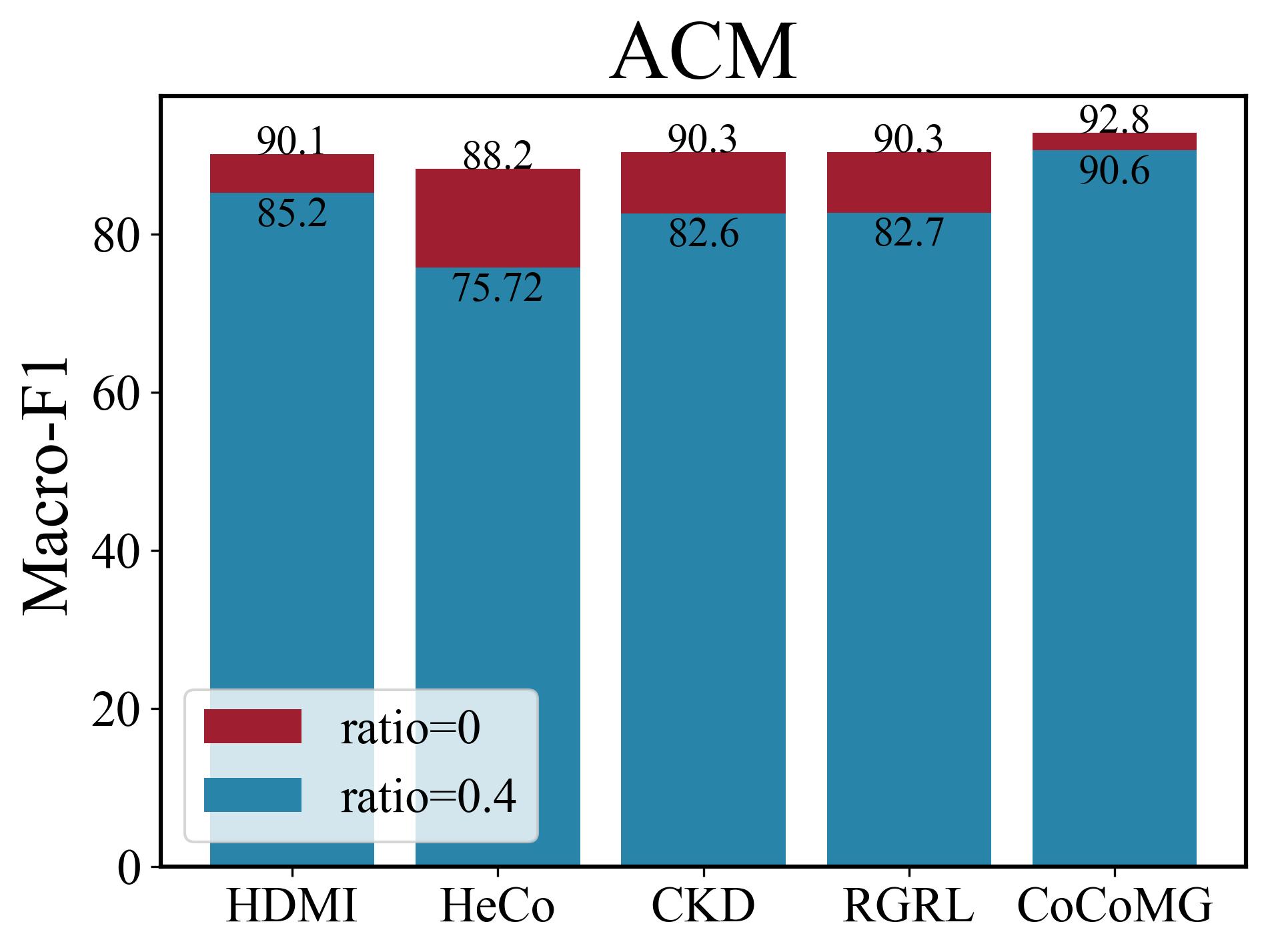
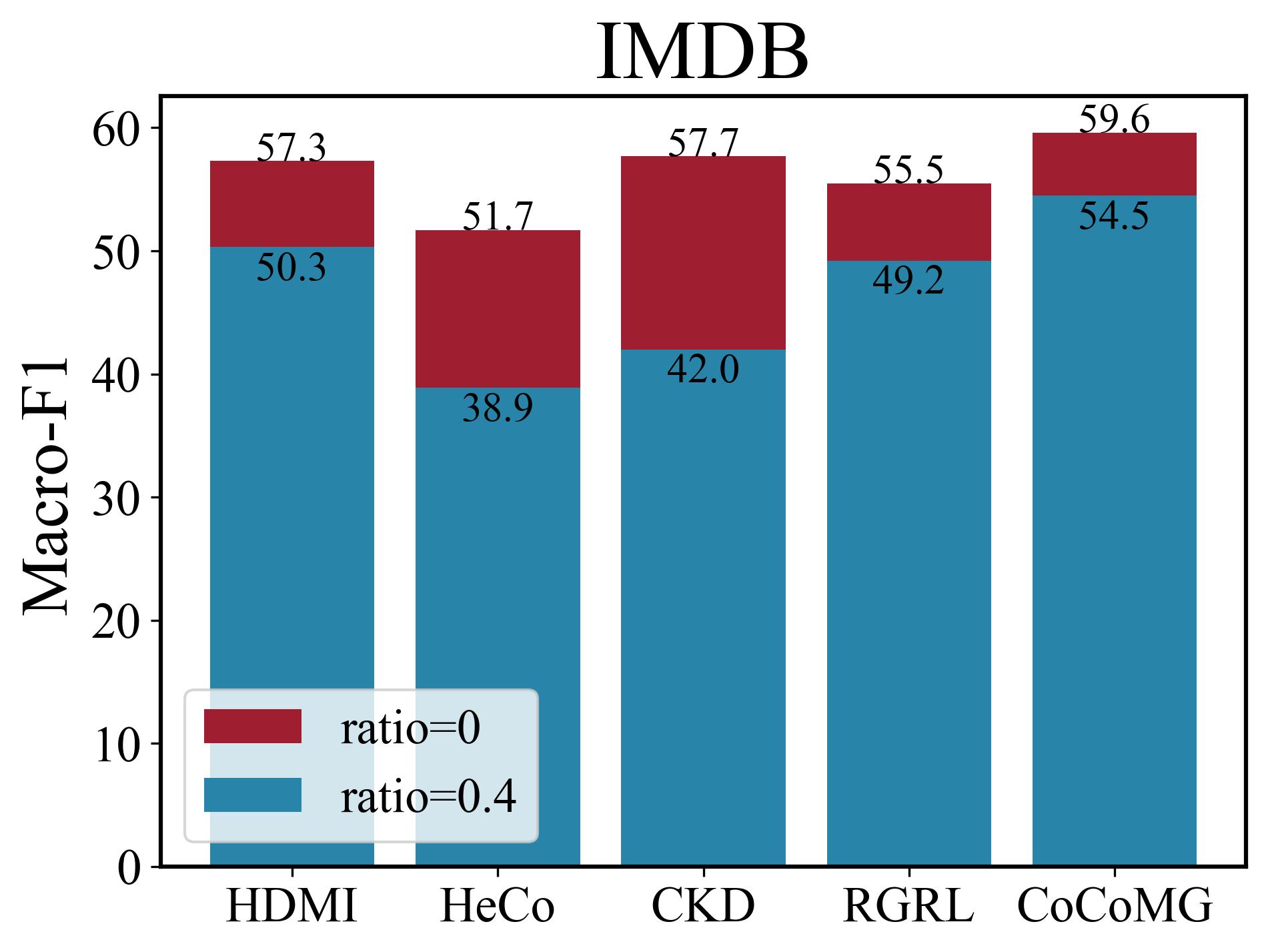
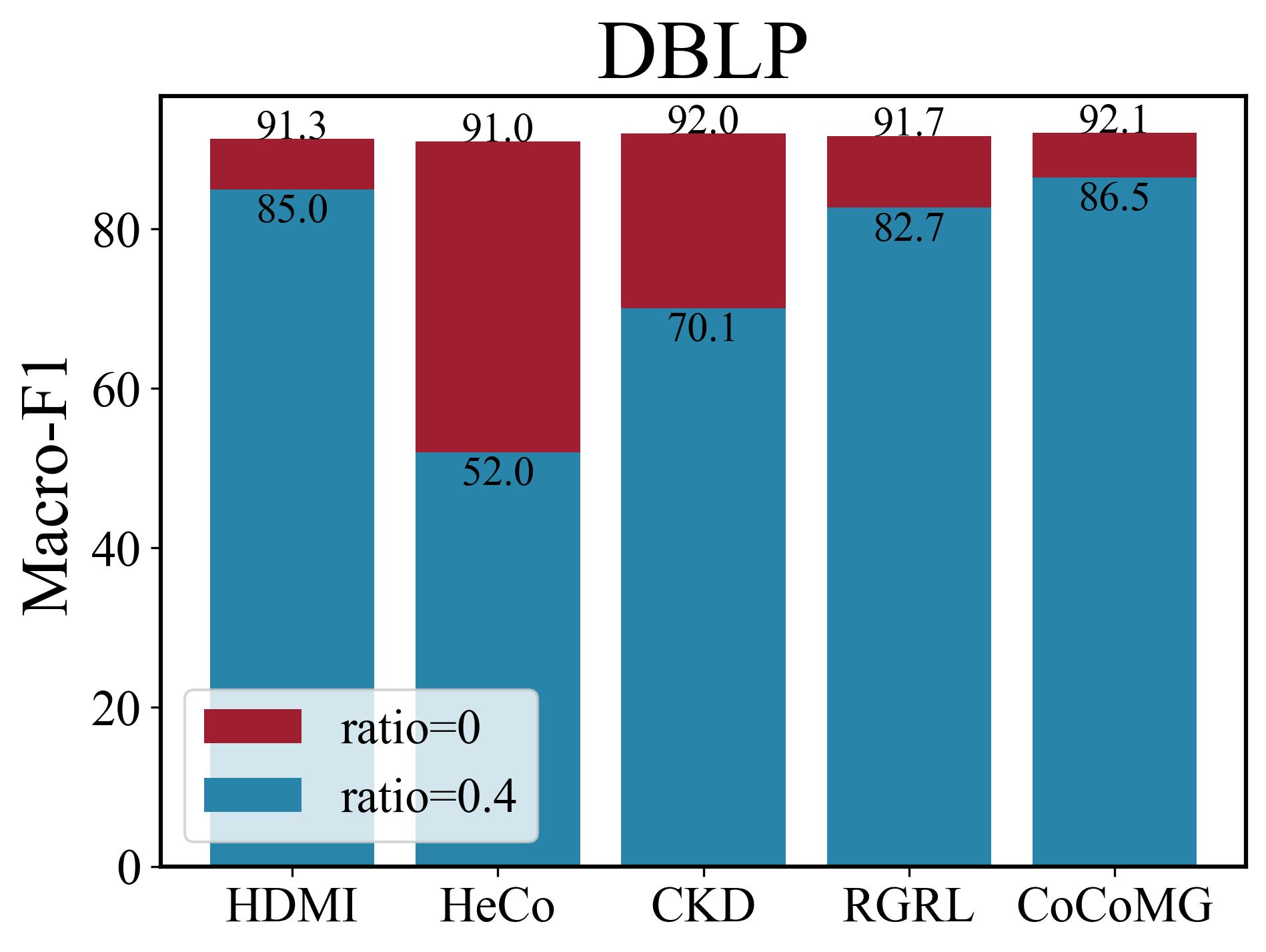
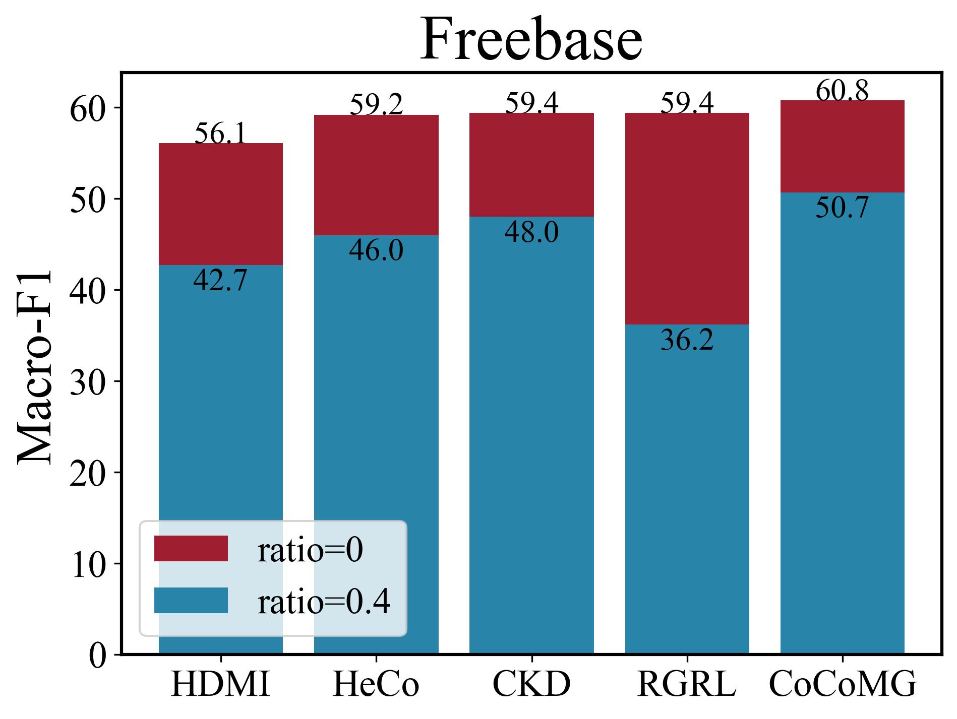
Figure 2. Classification performance of our method and four UMGL methods for the out-of-sample extension on all multiplex graph datasets. The “ratio” indicates the percentage of unseen nodes in each dataset.

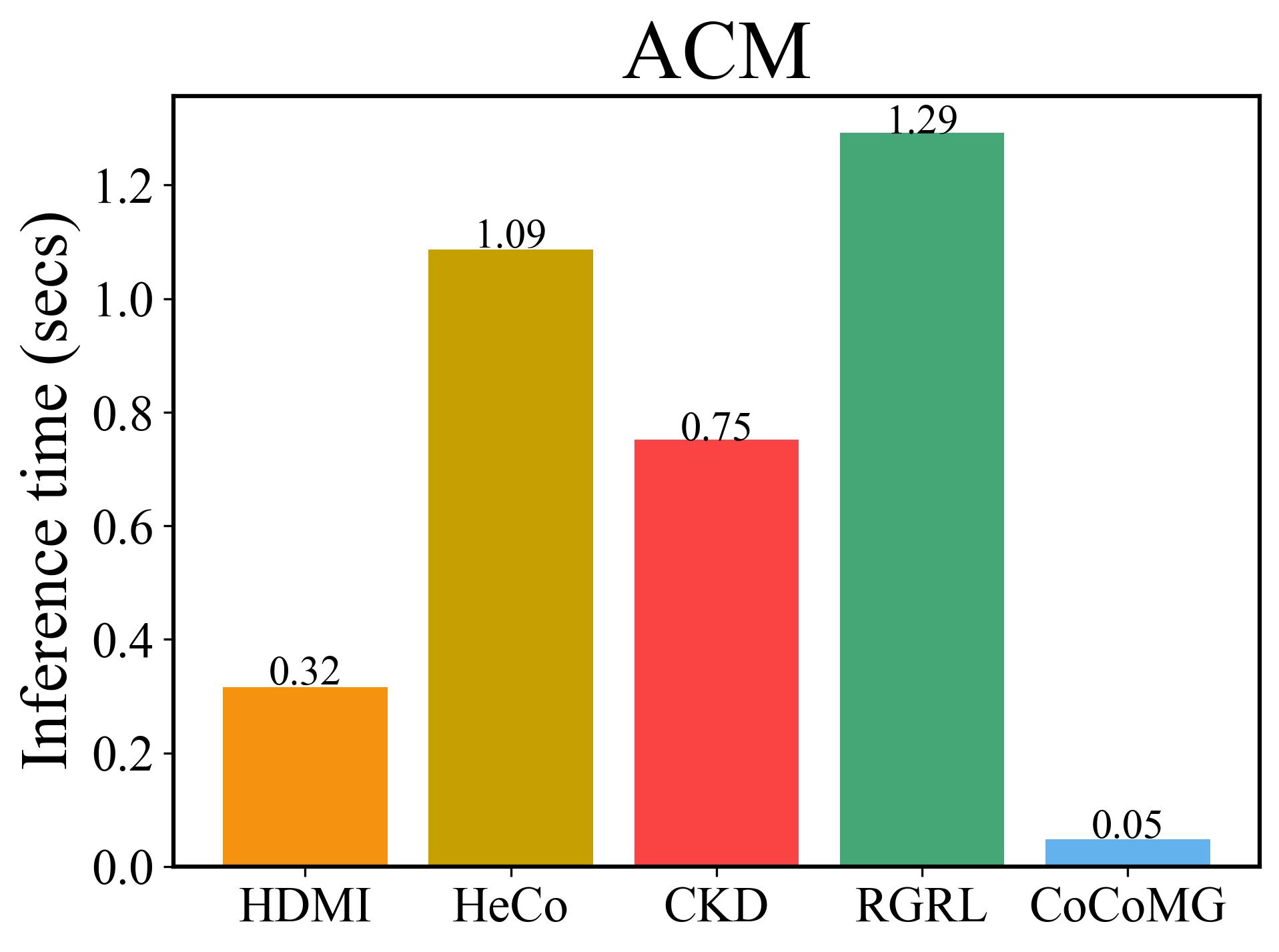
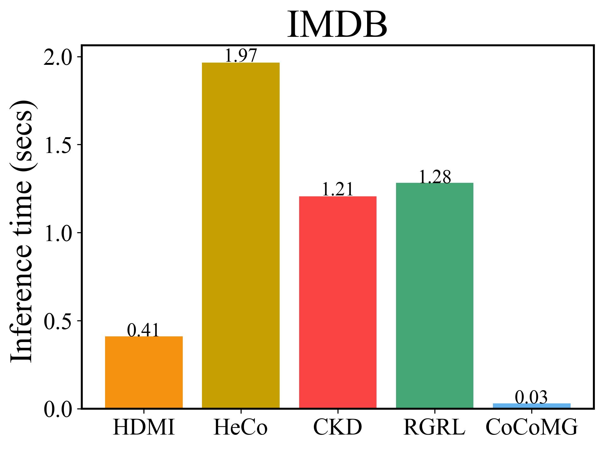
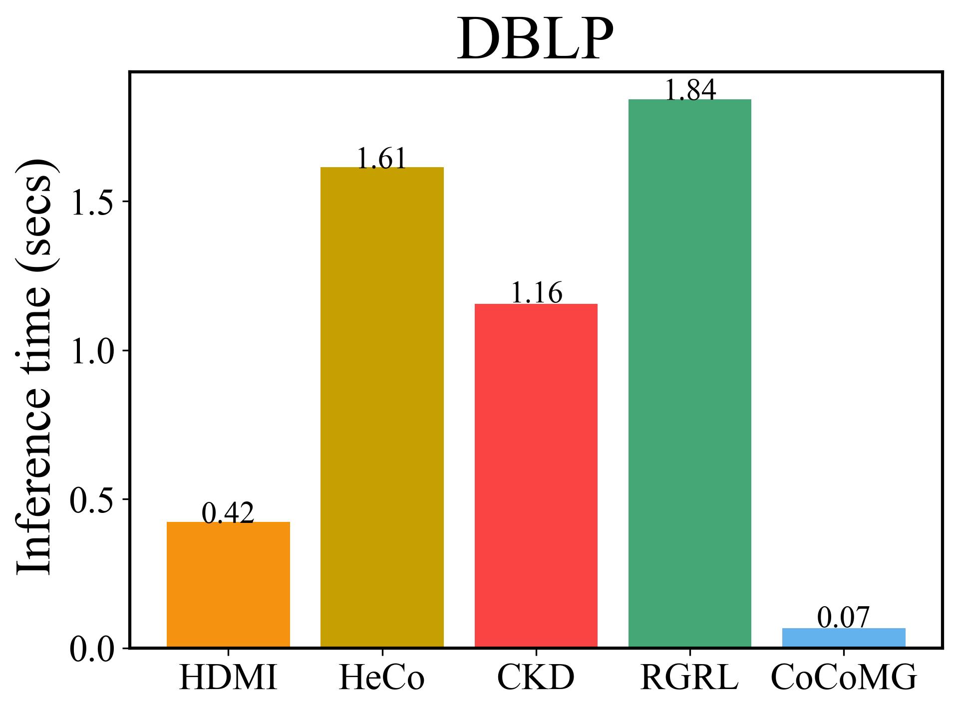
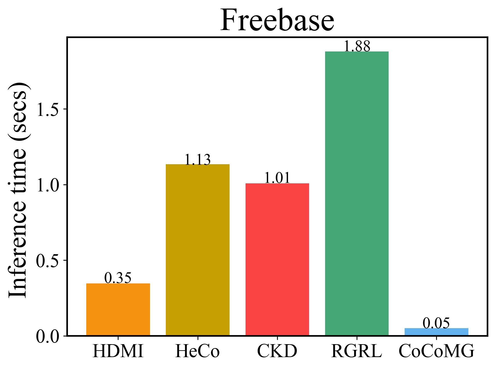
Figure 3. Inference time (seconds) of CoCoMG and four UMGL methods for the out-of-sample extension on all datasets.

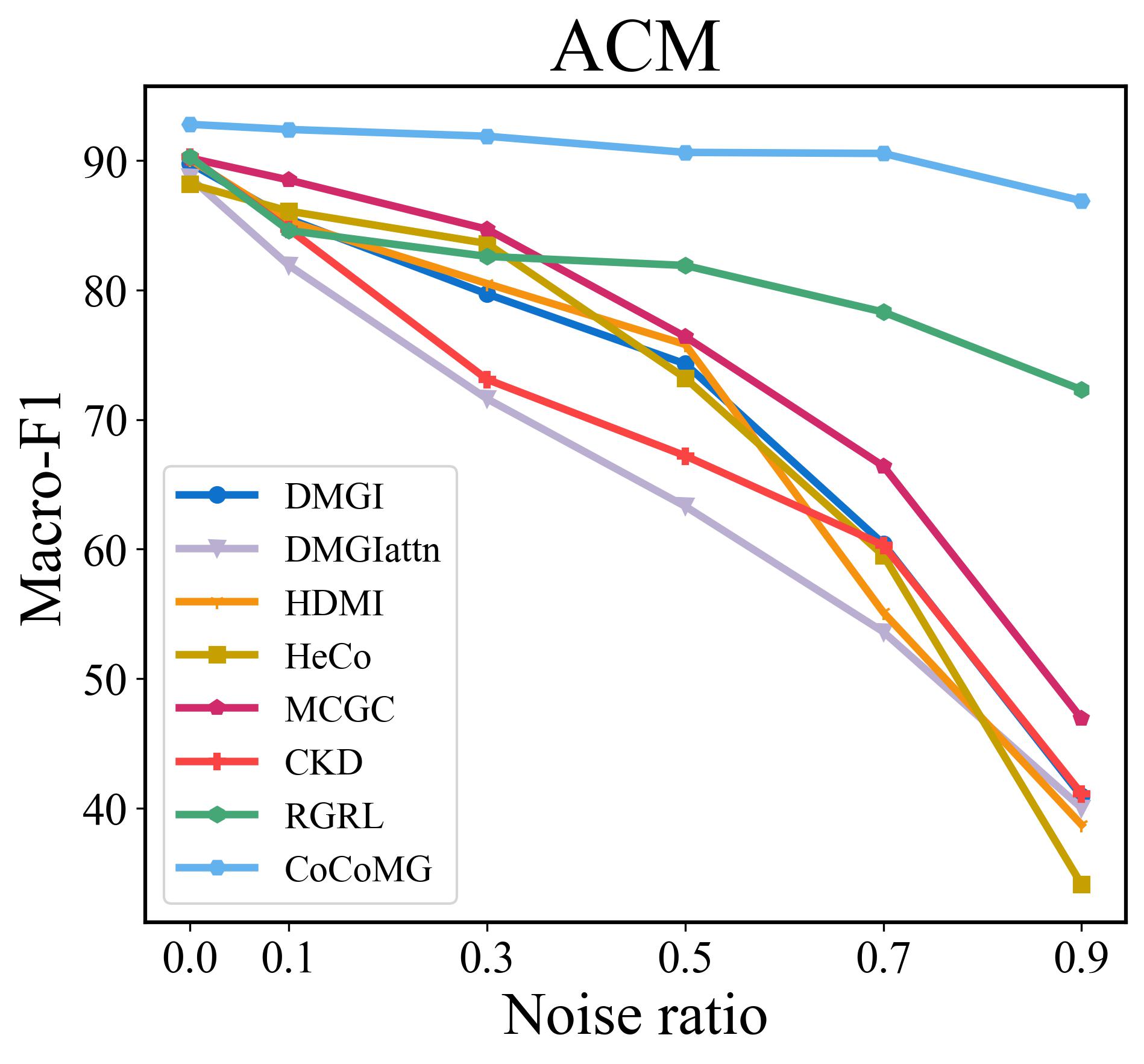
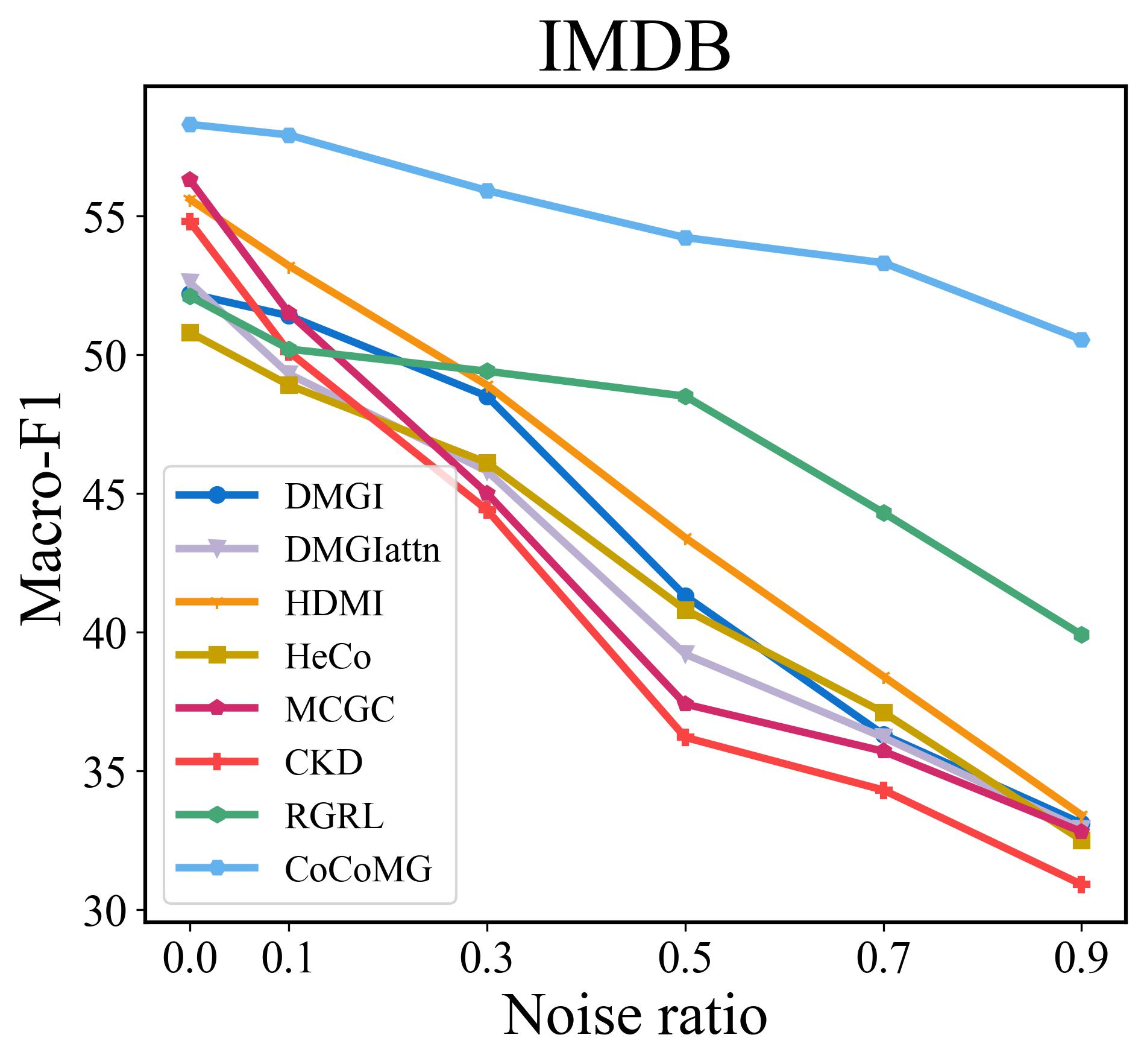
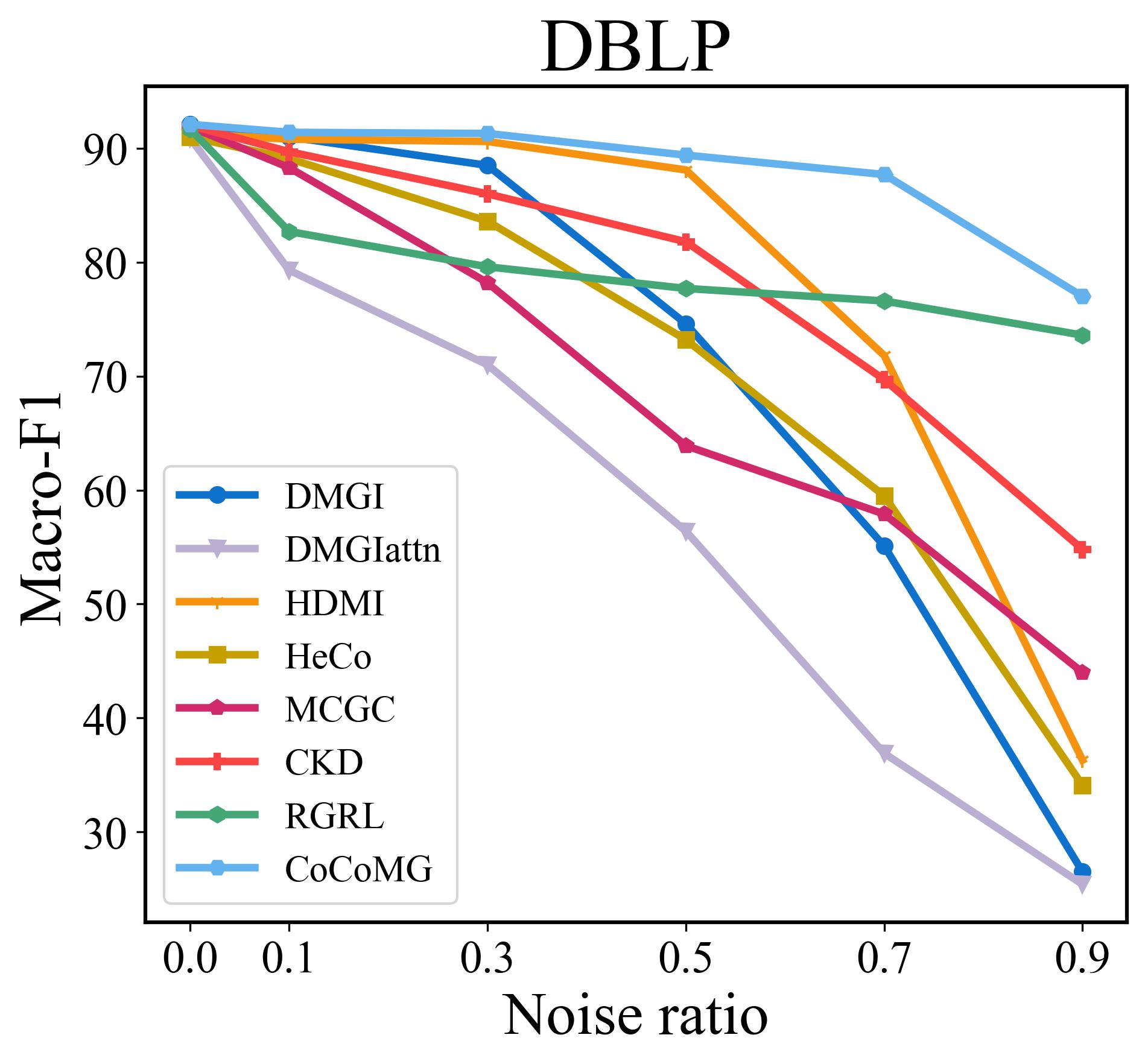
Figure 4. Classification performance of our method and all self-supervised multiplex graph representation methods under different noisy edges ratios $\eta$ on all multiplex graph datasets.

3. Experiments

3.1. Experimental Setup

3.1.1. Datasets

We use four public benchmark datasets to evaluate the performance of our proposed method, including two citation multiplex graph networks (i.e., ACM (Wang et al., 2019) and DBLP (Park et al., 2020)), and two movie multiplex graph networks (i.e., IMDB (Park et al., 2020) and Freebase (Jing et al., 2021)). We follow the public splitting settings (Jing et al., 2021; Wang et al., 2021) in our experiments.

3.1.2. Comparison methods

The comparison methods include four single-view graph learning methods and eight multiplex graph learning methods. The single-view graph learning methods consist of two semi-supervised methods, i.e., GCN (Kipf and Welling, 2017), and GAT (Velickovic et al., 2018), one traditional unsupervised learning method, i.e., DeepWalk (Perozzi et al., 2014), and one self-supervised learning method, i.e., DGI (Velickovic et al., 2019). The multiplex graph learning methods include one traditional unsupervised learning method,i.e., MNE (Zhang et al., 2018), and seven self-supervised learning methods, i.e., DMGI (Park et al., 2020), DMGIattn (Park et al., 2020), HDMI (Jing et al., 2021), HeCo (Wang et al., 2021), MCGC (Pan and Kang, 2021), CKD (Wang et al., 2022c), and RGRL (Lee et al., 2022). To ensure a fair comparison, we evaluate single-view graph methods on multiplex graph datasets by training them independently on each graph and then concatenating their learned representations for downstream tasks. The average values of 10 runs are reported.

3.1.3. Evaluation protocol

We follow the evaluation in previous works (Jing et al., 2021; Wang et al., 2022c) to conduct node classification and node clustering as semi-supervised and unsupervised downstream tasks, respectively. Specifically, we employ Macro-F1 and Micro-F1 to evaluate the performance of node classification. Moreover, we employ Accuracy and Normalized Mutual Information (NMI) to evaluate the performance of node clustering. Additionally, to evaluate the robustness of our method and comparison methods, we randomly replace a certain ratio of edges in each graph with noisy edges (i.e., random edges).

3.2. Effectiveness Analysis

To evaluate the effectiveness of the proposed method, we report the performance of node classification (i.e., Macro-F1 and Micro-F1) and node clustering (i.e., Accuracy and NMI) of all methods in Table 1 and 2, respectively. Obviously, the proposed method obtains the highest effectiveness on both node classification and node clustering tasks.

First, compared to the single graph learning methods (i.e., DeepWalk, GCN, GAT, and DGI), the proposed CoCoMG outperforms them by significant margins. For example, CoCoMG achieves an average improvement of 11.4% and 29.7% in terms of classification and clustering tasks, respectively, compared to the best-performing unsupervised single graph method DGI. Moreover, most multiplex graph learning methods have achieved better performance than single graph methods on both node classification and clustering tasks This suggests that multiplex graph learning methods are more effective than single-view graph methods, as they can explore the complementary and consistent information among different graphs to learn more discriminative node representations.

Second, compared to the multiplex graph learning methods, the proposed CoCoMG achieved the best performance, followed by CKD, MCGC, RGRL, HDMI, HeCo, DMGI, DMGIattn, and MNE. The reason can be attributed to that the proposed method can effectively extract complementary and consistent information while reducing the impact of noise.

3.3. Out-of-sample Analysis

In this section, we compare the effectiveness and efficiency of the proposed method with previous UMGL methods when tackling the out-of-sample issue. Note that, the comparison method, such as DMGI (Park et al., 2020), DMGIattn (Park et al., 2020), and MCGC (Pan and Kang, 2021), cannot handle the out-of-sample issue as they need to retrain the whole model to infer the representation of the unseen nodes. Thus, we only compare our method with HDMI (Jing et al., 2021), HeCo (Wang et al., 2021), CKD (Wang et al., 2022c), and RGRL (Lee et al., 2022) on all multiplex graph datasets. To do this, we first randomly split (repeated 5 times with random seeds) the unseen nodes from all nodes in the dataset with different ratios (i.e., 0 and 0.4) for each dataset. We then train the model for each method on the in-sample nodes with their local graph structures. After the training is completed, we use the optimized model to infer the representation of unseen nodes and evaluate the inference time and the performance on the node classification task.

The performance results are shown in Figure 2. Firstly, in terms of horizontal comparison (i.e., blue bars of all methods), the proposed method achieves the best performance on all datasets compared to the comparison methods, followed by HDMI, RGRL, CKD, and HeCo. Secondly, in terms of vertical comparison (i.e., the performance gap between red bars and blue bars), we observe that the performance drop of our method compared to the comparison methods is the least significant. The reason can be that previous methods only preserve the graph structure without learning an inference model that can map the input to the graph structure. As a result, these methods lack the inference ability when facing unseen nodes and their local graph structures. In contrast, our method learns an inference model that can implicitly map features to the graph structure, allowing it to effectively infer the representations of unseen nodes by implicitly mapping them to the graph structures among the seen nodes.

The inference times of our proposed method and comparison methods are presented in Figure 3, demonstrating the superior efficiency of our approach. Across all multiplex graph datasets, our method is on average 33.1× and 8.3× faster than the slowest method RGRL and the fastest method HDMI, respectively. This can be attributed to the fact that our method only utilizes MLP encoders for representation inference. These results are promising, as they indicate that our proposed method is capable of effectively tackling the out-of-sample issue while achieving superior efficiency.

Table 3. Classification performance (i.e., Macro-F1 and Micro-F1) of each constraint in CoCoMG on all mutiplex graph datasets.

		ACM		IMDB		DBLP		Freebase
$\mathcal{L}_{LP}$	$\mathcal{L}_{CCA}$	Macro-F1	Micro-F1	Macro-F1	Micro-F1	Macro-F1	Micro-F1	Macro-F1	Micro-F1
$-$	$\surd$	86.8 $\pm$ 0.8	86.9 $\pm$ 0.7	51.0 $\pm$ 0.4	51.6 $\pm$ 0.8	53.2 $\pm$ 0.2	77.9 $\pm$ 0.2	35.3 $\pm$ 0.3	42.7 $\pm$ 0.8
$\surd$	$-$	92.1 $\pm$ 0.2	92.1 $\pm$ 0.1	51.5 $\pm$ 0.6	52.1 $\pm$ 0.8	90.5 $\pm$ 0.4	91.5 $\pm$ 0.4	59.0 $\pm$ 0.5	62.4 $\pm$ 0.1
$\surd$	$\surd$	92.8 $\pm$ 0.1	92.7 $\pm$ 0.1	58.3 $\pm$ 0.4	59.6 $\pm$ 0.4	92.1 $\pm$ 0.1	92.9 $\pm$ 0.1	60.8 $\pm$ 0.1	63.8 $\pm$ 0.9

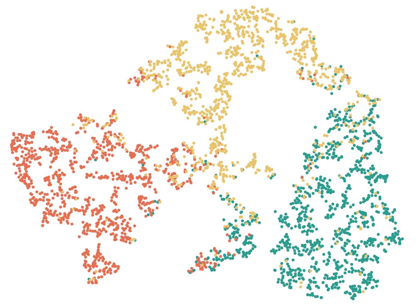
(a) w/o $\mathcal{L}_{LP}$(SIL=0.42)

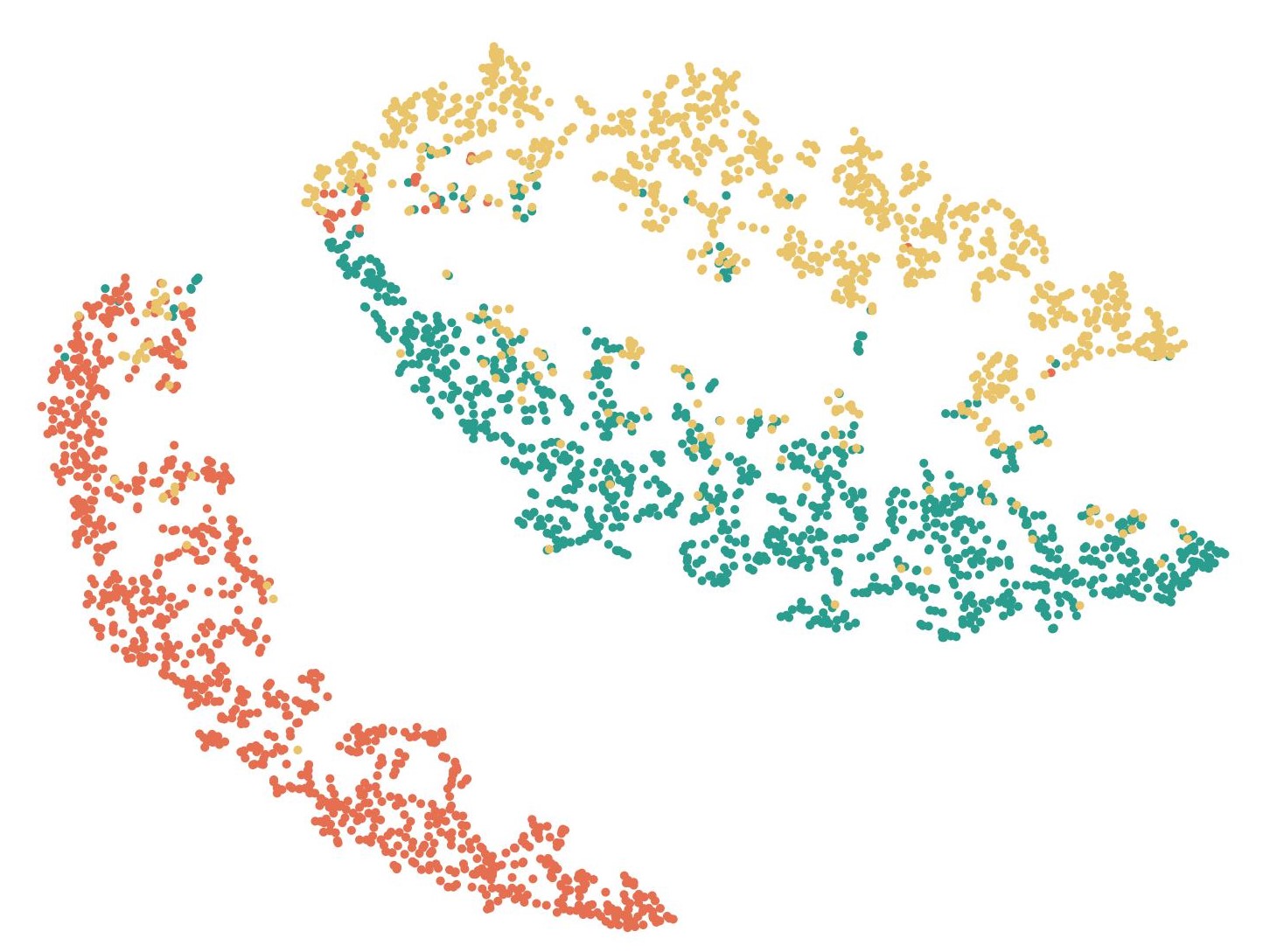
(b) w/o $\mathcal{L}_{CCA}$(SIL=0.53)

(c) with $\mathcal{J}$(SIL=0.74)

Figure 5. Visualization plotted by $t$-SNE and the corresponding silhouette scores (SIL) of node representations for our method on Dataset ACM, where different colors represent different classes of the nodes. (a) CoCoMG without $\mathcal{L}_{LP}$; (b) CoCoMG without $\mathcal{L}_{CCA}$; (c) CoCoMG with two constraints.

3.4. Robustness Analysis

To verify the robustness of the proposed method, we report the performance of all self-supervised multiplex graph learning methods on the node classification task under varying ratios of noisy edges (random edges) ranging from 0.1 to 0.9. These results are presented in Figure 4.

From Figure 4, we have the observations as follows. Firstly, the proposed method consistently achieves the best performance on all datasets under different noise ratios, confirming our claim that CoCoMG obtains satisfying prediction performance under noise. Secondly, as the noise ratio increases, the performance of all methods decreases, while the proposed method exhibits the smallest decrease. For instance, on Dataset ACM, the proposed method is minimally affected in terms of performance when the noise ratio is below 0.7. Even when the noise ratio reaches 0.9, the performance only decreases by approximately 6%, while other methods show a decrease of over 40%. The reasons behind these results are twofold. Firstly, we only use the MLP encoders to obtain node representations, which means noise cannot be directly aggregated into the node representations through incorrect edges. Secondly, we use Eq. (5) to ensure the consistency of the representations between different views, which reduces the noise caused by Eq. (2).

3.5. Ablation Study

The proposed method employs two constraints (i.e., $\mathcal{L}_{LP}$ in Eq. (2) and $\mathcal{L}_{CCA}$ in Eq. (5)) to extract complementary and consistent information, respectively. To verify the effectiveness of each constraint of the proposed method, we investigate the performance(i.e., Macro-F1 and Micro-F1) of each constraint on the node classification task, and report the results in Table 3. Generally, we observe that the proposed method with two constraints achieves the best performance. Conversely, when we only implement an individual constraint (i.e., either $\mathcal{L}_{LP}$ or $\mathcal{L}_{CCA}$), the performance is inferior. Moreover, as shown in Figure 5, we utilize $t$-SNE (Van der Maaten and Hinton, 2008) to visualize the node representations learned with different constraints on the ACM dataset. We observed that the representations of nodes belonging to the same class, learned with both constraints, are closer to each other than the representations learned with only one constraint. Consequently, the experiments confirm that both constraints play a crucial role in the effectiveness of CoCoMG.

3.6. Over-smooth Analysis

Previous UMGL methods have relied heavily on GCN to obtain node embeddings. However, as the number of layers in a GCN increases, the performance of the model tends to decrease, which is known as the over-smooth problem. In fact, modern deep neural networks typically require multiple layers to effectively extract features and learn complex patterns, but in graph neural networks, using too many graph convolutional layers can lead to the over-smooth phenomenon, which limits the number of layers in a GCN. To some extent, this presents a paradoxical situation in which the depth of the GCN is both necessary and limited.

In this section, we analyze the effectiveness of the proposed method when dealing with the over-smooth problem. For this purpose, we evaluate the effectiveness of our method and vanilla GCN (i.e., using GCN as encoder) with varying numbers of layers ranging from $1$ to $19$ on Dataset ACM, and the results are presented in Figure 6. Overall, the performance of our method shows a slight increase and remains stable with the number of layers increasing, while vanilla GCN’s performance drops sharply. Specifically, our model’s performance improves as the number of layers increases from $1$ to $11$, and the performance of our model remains stable with the increase in the number of layers from $11$ to $19$. In contrast, for vanilla GCN, the performance drops significantly with the number of layers from $1$ to $19$, with a drop of over 60%. The reason might be as follows. For our model, as the number of layers increases, the model can learn more abstract node embeddings, and thus the performance of the model increases gradually. For vanilla GCN, however, the message passing mechanism causes the node embeddings to become more and more similar as the layers increase, significantly degrading performance. Based on this observation, we can conclude that our method can effectively address the over-smoothing problem.

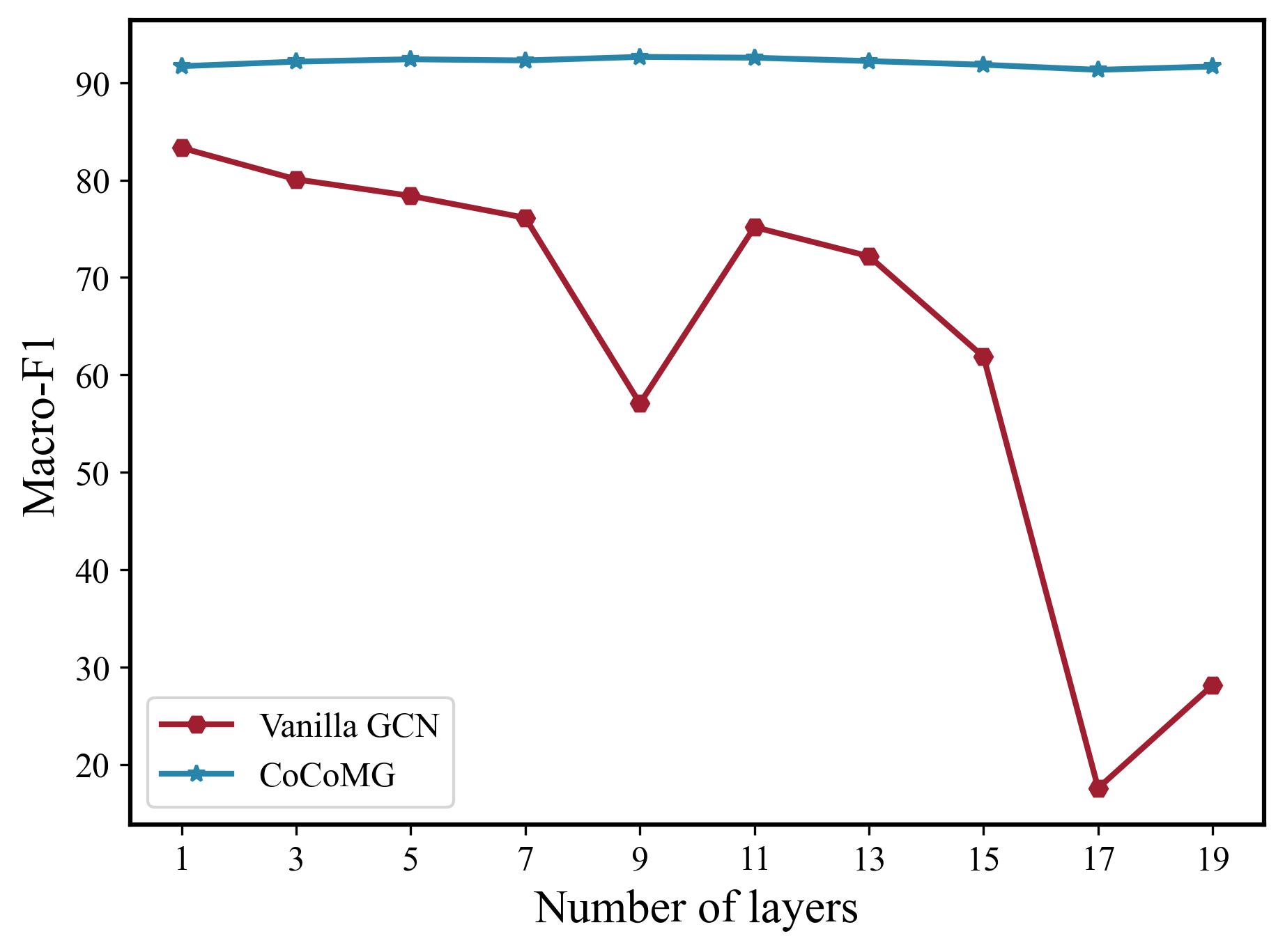
Figure 6. Classification results of our method and vanilla GCN under different number of layers on Dataset ACM

3.7. Parameter Sensitivity

The hyper-parameter of CoCoMG includes the trade-off $\gamma$ in Eq. (5) and $\beta$ in Eq. (6), and Figure 7 shows the effectiveness by traversing $\gamma$ and $\beta$ on Dataset ACM. The results indicate that $\beta$ is relatively insensitive in the range of 0.01 to 10, while $\gamma$ exhibits little sensitivity to performance. These results suggest that CoCoMG can achieve near-perfect performance when the value of $\gamma$ is in a reasonable range (e.g., $\gamma>0.1$).

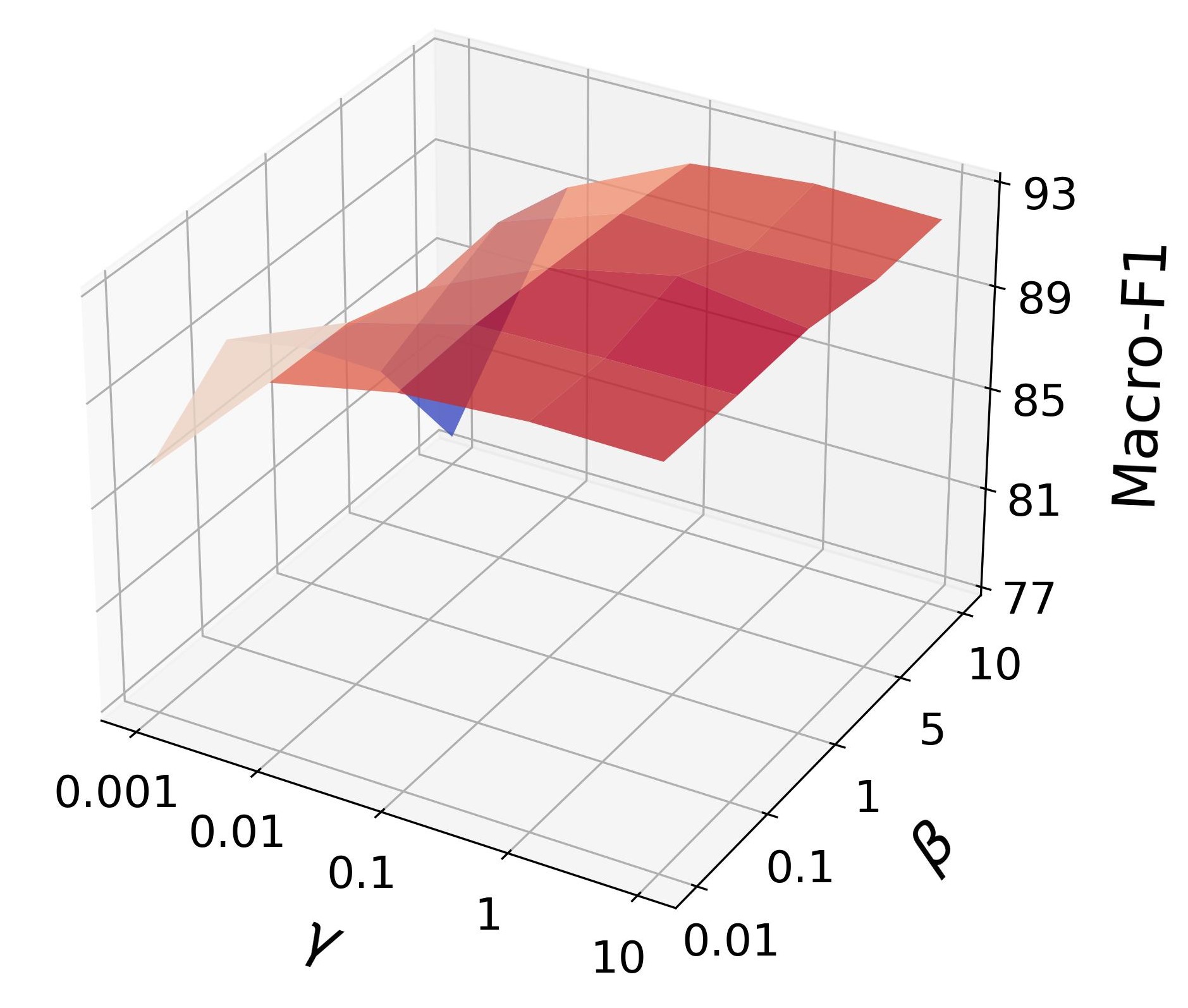
Figure 7. Classification results of our method at different parameter settings (i.e., $\gamma$ and $\beta$) on Dataset ACM.

4. Conclusion

In this paper, we investigated two pervasive but challenging issues of existing UMGL methods, i.e., the out-of-sample issue and the noise issue. To tackle these issues, we proposed CoCoMG, that only employs multiple MLP encoders with two constraints to effectively and efficiently extract complementary and consistent information for conducting unsupervised multiple graph learning. Comprehensive experiments demonstrate that CoCoMG achieves state-of-the-art performance in terms of both effectiveness and efficiency, as well as confirm our claim that CoCoMG can tackle those two issues.

References

- (1)
- Battiston et al. (2017) Federico Battiston, Vincenzo Nicosia, and Vito Latora. 2017. The new challenges of multiplex networks: Measures and models. The European Physical Journal Special Topics 226 (2017), 401–416.
- Cen et al. (2019) Yukuo Cen, Xu Zou, Jianwei Zhang, Hongxia Yang, Jingren Zhou, and Jie Tang. 2019. Representation learning for attributed multiplex heterogeneous network. In KDD. 1358–1368.
- Chu et al. (2019) Xiaokai Chu, Xinxin Fan, Di Yao, Zhihua Zhu, Jianhui Huang, and Jingping Bi. 2019. Cross-Network Embedding for Multi-Network Alignment. In WWW. 273–284.
- Dong et al. (2016) Xiaowen Dong, Dorina Thanou, Pascal Frossard, and Pierre Vandergheynst. 2016. Learning Laplacian Matrix in Smooth Graph Signal Representations. IEEE Transactions on Signal Process. 64, 23 (2016), 6160–6173.
- Gan et al. (2022) Jiangzhang Gan, Rongyao Hu, Yujie Mo, Zhao Kang, Liang Peng, Yonghua Zhu, and Xiaofeng Zhu. 2022. Multi-graph Fusion for Dynamic Graph Convolutional Network. IEEE Transactions on Neural Networks and Learning Systems (2022), 10.1109/TNNLS.2022.3172588.
- Hamilton et al. (2017) William L. Hamilton, Zhitao Ying, and Jure Leskovec. 2017. Inductive Representation Learning on Large Graphs. In NeurIPS. 1024–1034.
- Han et al. (2023) Beibei Han, Yingmei Wei, Qingyong Wang, and Shanshan Wan. 2023. CoLM2S: Contrastive self-supervised learning on attributed multiplex graph network with multi-scale information. CAAI Transactions on Intelligence Technology (2023).
- Hardoon et al. (2004) David R. Hardoon, Sándor Szedmák, and John Shawe-Taylor. 2004. Canonical correlation analysis: An overview with application to learning methods. Neural Computing. 16, 12 (2004), 2639–2664.
- Jing et al. (2022a) Baoyu Jing, Shengyu Feng, Yuejia Xiang, Xi Chen, Yu Chen, and Hanghang Tong. 2022a. X-GOAL: Multiplex Heterogeneous Graph Prototypical Contrastive Learning. In CIKM. 894–904.
- Jing et al. (2021) Baoyu Jing, Chanyoung Park, and Hanghang Tong. 2021. HDMI: High-order Deep Multiplex Infomax. In WWW. 2414–2424.
- Jing et al. (2022b) Li Jing, Pascal Vincent, Yann LeCun, and Yuandong Tian. 2022b. Understanding Dimensional Collapse in Contrastive Self-supervised Learning. In ICLR.
- Kipf and Welling (2016) Thomas N Kipf and Max Welling. 2016. Variational graph auto-encoders. arXiv preprint arXiv:1611.07308 (2016).
- Kipf and Welling (2017) Thomas N. Kipf and Max Welling. 2017. Semi-Supervised Classification with Graph Convolutional Networks. In ICLR. 1–14.
- LeCun et al. (2015) Yann LeCun, Yoshua Bengio, and Geoffrey Hinton. 2015. Deep learning. Nature 521, 7553 (2015), 436–444.
- Lee et al. (2022) Namkyeong Lee, Dongmin Hyun, Junseok Lee, and Chanyoung Park. 2022. Relational Self-Supervised Learning on Graphs. In CIKM. 1054–1063.
- Li et al. (2021) Zhiqiang Li, Hao Wang, and Jian Zhang. 2021. A multiplex graph learning framework for predicting drug-disease associations. IEEE/ACM Transactions on Computational Biology and Bioinformatics 18, 3 (2021), 807–818.
- Liu et al. (2022) Yixin Liu, Shirui Pan, Ming Jin, Chuan Zhou, Feng Xia, and Philip S Yu. 2022. Graph self-supervised learning: A survey. IEEE Transactions on Knowledge and Data Engineering (2022), 1–1.
- Ma et al. (2018) Jianxin Ma, Peng Cui, and Wenwu Zhu. 2018. DepthLGP: Learning Embeddings of Out-of-Sample Nodes in Dynamic Networks. In AAAI. 370–377.
- Oord et al. (2018) Aaron van den Oord, Yazhe Li, and Oriol Vinyals. 2018. Representation learning with contrastive predictive coding. arXiv preprint arXiv:1807.03748 (2018).
- Pan and Kang (2021) Erlin Pan and Zhao Kang. 2021. Multi-view Contrastive Graph Clustering. In NeurIPS. 2148–2159.
- Park et al. (2020) Chanyoung Park, Donghyun Kim, Jiawei Han, and Hwanjo Yu. 2020. Unsupervised Attributed Multiplex Network Embedding. In AAAI. 5371–5378.
- Peng et al. (2022) Liang Peng, Rongyao Hu, Fei Kong, Jiangzhang Gan, Yujie Mo, Xiaoshuang Shi, and Xiaofeng Zhu. 2022. Reverse Graph Learning for Graph Neural Network. IEEE Transactions on Neural Networks and Learning Systems (2022), 1–12. https://doi.org/10.1109/TNNLS.2022.3161030
- Perozzi et al. (2014) Bryan Perozzi, Rami Al-Rfou, and Steven Skiena. 2014. Deepwalk: Online learning of social representations. In KDD. 701–710.
- Van der Maaten and Hinton (2008) Laurens Van der Maaten and Geoffrey Hinton. 2008. Visualizing data using t-SNE. Journal of Machine Learning Research 9, 11 (2008).
- Vaswani et al. (2017) Ashish Vaswani, Noam Shazeer, Niki Parmar, Jakob Uszkoreit, Llion Jones, Aidan N Gomez, Ł ukasz Kaiser, and Illia Polosukhin. 2017. Attention is All you Need. In NeurIPS, Vol. 30.
- Veličković (2022) Petar Veličković. 2022. Message passing all the way up. arXiv preprint arXiv:2202.11097 (2022).
- Velickovic et al. (2018) Petar Velickovic, Guillem Cucurull, Arantxa Casanova, Adriana Romero, Pietro Liò, and Yoshua Bengio. 2018. Graph Attention Networks. In ICLR. 1–12.
- Velickovic et al. (2019) Petar Velickovic, William Fedus, William L. Hamilton, Pietro Liò, Yoshua Bengio, and R. Devon Hjelm. 2019. Deep Graph Infomax. In ICLR. 1–17.
- Wang et al. (2022c) Can Wang, Sheng Zhou, Kang Yu, Defang Chen, Bolang Li, Yan Feng, and Chun Chen. 2022c. Collaborative Knowledge Distillation for Heterogeneous Information Network Embedding. In WWW. 1631–1639.
- Wang et al. (2022a) Haoqing Wang, Xun Guo, Zhi-Hong Deng, and Yan Lu. 2022a. Rethinking Minimal Sufficient Representation in Contrastive Learning. In CVPR. IEEE, 16020–16029.
- Wang et al. (2022b) Qiang Wang, Hao Jiang, Ying Jiang, Shuwen Yi, Qi Nie, and Geng Zhang. 2022b. Multiplex network infomax: Multiplex network embedding via information fusion. Digital Communications and Networks (2022).
- Wang et al. (2019) Xiao Wang, Houye Ji, Chuan Shi, Bai Wang, Yanfang Ye, Peng Cui, and Philip S. Yu. 2019. Heterogeneous Graph Attention Network. In WWW. 2022–2032.
- Wang et al. (2021) Xiao Wang, Nian Liu, Hui Han, and Chuan Shi. 2021. Self-supervised Heterogeneous Graph Neural Network with Co-contrastive Learning. In KDD. 1726–1736.
- Xie et al. (2023) Yaochen Xie, Zhao Xu, Jingtun Zhang, Zhengyang Wang, and Shuiwang Ji. 2023. Self-Supervised Learning of Graph Neural Networks: A Unified Review. IEEE Transactions on Pattern Analysis and Machine Intelligence 45, 2 (2023), 2412–2429.
- Yuan et al. (2021) Changan Yuan, Zhi Zhong, Cong Lei, Xiaofeng Zhu, and Rongyao Hu. 2021. Adaptive reverse graph learning for robust subspace learning. Information Processing & Management 58, 6 (2021), 102733.
- Zhang et al. (2018) Hongming Zhang, Liwei Qiu, Lingling Yi, and Yangqiu Song. 2018. Scalable Multiplex Network Embedding. In IJCAI. 3082–3088.
- Zhang et al. (2019) Jun Zhang, Peng Cui, Xiao Wang, and Wenwu Zhu. 2019. Multiplex graph learning: Algorithms and applications. IEEE Transactions on Neural Networks and Learning Systems 30, 1 (2019), 14–28.
- Zhang et al. (2023) Qiqi Zhang, Zhongying Zhao, Hui Zhou, Xiangju Li, and Chao Li. 2023. Self-supervised Contrastive Learning on Heterogeneous Graphs with Mutual Constraints of Structure and Feature. Information Sciences (2023), 119026.
- Zhang et al. (2022) Rui Zhang, Arthur Zimek, and Peter Schneider-Kamp. 2022. Unsupervised Representation Learning on Attributed Multiplex Network. In CIKM. 2610–2619.
- Zhao et al. (2017) Jing Zhao, Xijiong Xie, Xin Xu, and Shiliang Sun. 2017. Multi-view learning overview: Recent progress and new challenges. Information Fusion 38 (2017), 43–54.
- Zhou et al. (2020) Daokun Zhou, Wei Bao, and Wei Liu. 2020. Multiple graph learning: An unsupervised feature learning approach for graph-structured data. IEEE Transactions on Neural Networks and Learning Systems 31, 7 (2020), 2632–2642.
- Zhu et al. (2018) Dingyuan Zhu, Peng Cui, Ziwei Zhang, Jian Pei, and Wenwu Zhu. 2018. High-order proximity preserved embedding for dynamic networks. IEEE Transactions on Knowledge and Data Engineering 30, 11 (2018), 2134–2144.
- Zhu et al. (2022a) Yonghua Zhu, Junbo Ma, Changan Yuan, and Xiaofeng Zhu. 2022a. Interpretable learning based Dynamic Graph Convolutional Networks for Alzheimer’s Disease analysis. Information Fusion 77 (2022), 53–61.
- Zhu et al. (2022b) Yanqiao Zhu, Yichen Xu, Hejie Cui, Carl Yang, Qiang Liu, and Shu Wu. 2022b. Structure-Enhanced Heterogeneous Graph Contrastive Learning. In ICDM. 82–90.
- Zhu et al. (2021) Yanqiao Zhu, Yichen Xu, Feng Yu, Qiang Liu, Shu Wu, and Liang Wang. 2021. Graph contrastive learning with adaptive augmentation. In WWW. 2069–2080.