Krylov Solvers for Interior Point Methods with Applications in Radiation Therapy

Abstract

Interior point methods are widely used for different types of mathematical optimization problems. Many implementations of interior point methods in use today rely on direct linear solvers to solve systems of equations in each iteration. The need to solve ever larger optimization problems more efficiently and the rise of hardware accelerators for general purpose computing has led to a large interest in using iterative linear solvers instead, with the major issue being inevitable ill-conditioning of the linear systems arising as the optimization progresses. We investigate the use of Krylov solvers for interior point methods in solving optimization problems from radiation therapy. We implement a prototype interior point method using a so called doubly augmented formulation of the Karush-Kuhn-Tucker (KKT) linear system of equations, originally proposed by Forsgren and Gill, and evaluate its performance on real optimization problems from radiation therapy. Crucially, our implementation uses a preconditioned conjugate gradient method with Jacobi preconditioning internally. Our measurements of the conditioning of the linear systems indicate that the Jacobi preconditioner improves the conditioning of the systems to a degree that they can be solved iteratively, but there is room for further improvement in that regard. Furthermore, profiling of our prototype code shows that it is suitable for GPU acceleration, which may further improve its performance in practice. Overall, our results indicate that our method can find solutions of acceptable accuracy in reasonable time, even with a simple Jacobi preconditioner.

1 Introduction

Mathematical optimization is used in many areas of science and industry, with applications in fields like precision medicine, operations research and many others. In this paper, we are concerned with optimization problems from treatment planning for radiation therapy, where optimization is used to find optimal treatment plans tailored to each individual patient. Such optimization problems are often large in size and can require significant computational effort to solve. The specific nature of the optimization problems from this domain vary depending on multiple factors, including choices made in modeling the optimization problems, the modality of treatment (using photons or protons, for instance), and others. In general, we are interested in continuous, constrained nonlinear optimization problems that are solved using sequential quadratic programming. At each step in the algorithm, a quadratic programming (QP) subproblem is solved using an interior point method, which represents the main computational burden in the solver. Thus, the focus of this paper lies on interior point methods for solving QPs using iterative linear solvers.

Computationally, primal-dual interior point methods for optimization rely on Newton’s method to find search directions. This involves the solution of a large, often sparse and structured linear system of equations, which we will refer to henceforth as the KKT-system, at each iteration. Traditionally, this system is often solved using direct linear solvers, such as $LDL^{T}$-factorization for indefinite matrices, but a topic of interest for much research in the field is the use of iterative linear solvers [22], such as Krylov subspace methods, instead. The main advantage from using iterative linear solvers over direct ones is their superior parallel scaling properties and ability to handle much larger problems. Indeed, the move to iterative linear algebra for interior point methods has been identified by some authors as a key step in enabling interior point methods to handle very large optimization problems [14].

Another key advantage of iterative algorithms for solving linear systems is their suitability for modern computing hardware, such as GPUs. With their rising dominance in High-Performance Computing (HPC), extracting the maximum performance from modern computing hardware all but requires the use of some type of accelerator. In contrast, direct linear solvers can suffer performance wise on these types of hardware for a variety of reasons, e.g. unstructured memory accesses or others. This performance bottleneck has been seen in previous studies [25] in the context of interior point methods. The major challenge of using iterative solvers in this context, however, lies in a structured form of ill-conditioning that inevitably exists in the linear systems, which can be severely detrimental to the convergence of the linear solver. Still, given potential performance gains from the use of significantly more powerful computing resources, we believe the trade-off between numerical stability and parallel performance is worthy of further investigation.

In this paper, we investigate the possibility of using iterative linear solvers in an interior point method for QP subproblems arising from real world optimization problems in radiation treatment planning. Our method is based on the work by Forsgren and Gill in [9], where a special formulation of the KKT systems from interior point methods is considered, which guarantees that the KKT system is positive-definite throughout the optimization for convex problems. We implement an interior-point solver prototype code which uses the preconditioned conjugate gradient method to solve the linear systems, and evaluate its performance and convergence properties on real world problems.

2 Background

2.1 Interior Point Methods

We are concerned with the solution of convex, continuous quadratic programs using interior point methods. The following section introduces the relevant aspects for our proposed method. Readers interested in a more thorough overview of interior point methods for optimization are referred to e.g. [26, 11]. In general, we will be dealing with a problem on the form:

(2.1) min. $$\quad\frac{1}{2}x^{T}Hx+p^{T}x$$

s.t. $$\quad l\leq Ax\leq u,$$

where $H$ is the (positive definite) Hessian of the objective function, $p\in\mathbb{R}^{n}$ are the linear coefficients of the objective, and $A$ is the Jacobian of the (linear) constraints. In general, we allow components of the constraints to be unbounded, but we do not account for this explicitly to simplify the exposition. Inequality constraints are often treated by the introduction of auxiliary slack variables. Converting the problem to having only lower bounds and introduction of slack variables $s_{l},s_{u}$ (for lower and upper bounds respectively) gives:

(2.2) min. $$\frac{1}{2}x^{T}Hx+p^{T}x$$

s.t. $$Ax-s_{l}-l=0$$

$$- Ax-s_{u}+u=0$$

$$s_{l},s_{u}\geq 0.$$

Interior point methods handle inequality constraints by replacing them with a logarithmic barrier-term in the objective, giving rise to a purely equality-constrained barrier subproblem in our case:

(2.3) min. $$\frac{1}{2}x^{T}Hx+p^{T}x-$$

$$-\mu\sum\log((s_{l})_{i})-\mu\sum\log((s_{u})_{i})$$

s.t. $$Ax-s_{l}-l=0$$

$$- Ax-s_{u}+u=0.$$

Here $\mu$ is the so called barrier parameter. Intuitively, the barrier terms diverge towards $+\infty$ as the boundary of the feasible set is approached, thus encouraging feasibility throughout the iterations. As is common in primal-dual interior point methods, we work with the perturbed optimality conditions. These state that an optimal solution to the equality constrained subproblem in (2.3) satisfies the following:

(2.4) $$Hx+p-A^{T}\lambda_{l}+A^{T}\lambda_{u}=0$$

(2.5) $$Ax-s_{l}-l=0$$

(2.6) $$-Ax+s_{u}+u=0$$

(2.7) $$(\lambda_{l})_{i}(s_{l})_{i}=\mu\quad i=1,...,m_{l}$$

(2.8) $$(\lambda_{l})_{i}(s_{u})_{i}=\mu\quad i=1,...,m_{l}.$$

These conditions are the same as the first order Karush-Kuhn Tucker (KKT) conditions for optimality (for problem (2.2)), except that the final two conditions are perturbed by $\mu$. Interior point methods generally seek points satisfying the perturbed optimality conditions above, while successively decreasing the barrier parameter $\mu\rightarrow 0$. As $\mu$ approaches $0$, we expect our solution to approach a point satisfying the KKT conditions for optimality.

Many optimization problems also include lower and upper bounds on the variables $x$ directly. Such bounds can be included by the introduction of appropriate rows in the $A$ matrix. However, the linear algebra can often be simplified when separate handling of the bounds on the variables from general linear constraints is used. Separating the variable bounds from the general linear constraints gives us the following set of optimality conditions, written in a form suitable for solving using Newton’s method:

$$r_{H}\coloneqq Hx+p-A^{T}\lambda_{l_{A}}+A^{T}\lambda_{u_{A}}-\lambda_{l_{x}}+\lambda_{u_{x}}=0$$

$$r_{A_{l}}\coloneqq Ax-s_{l_{A}}-l_{A}=0$$

$$r_{A_{u}}\coloneqq-Ax-s_{u_{A}}+u_{A}=0$$

$$r_{l_{x}}\coloneqq x-s_{l_{x}}-l_{x}=0$$

$$r_{u_{x}}\coloneqq-x-s_{u_{x}}+u_{x}=0$$

$$r_{c_{1}}\coloneqq\Lambda_{l_{A}}S_{l_{A}}-\mu e=0$$

$$r_{c_{2}}\coloneqq\Lambda_{u_{A}}S_{u_{A}}-\mu e=0$$

$$r_{c_{3}}\coloneqq\Lambda_{l_{x}}S_{l_{x}}-\mu e=0$$

$$r_{c_{4}}\coloneqq\Lambda_{u_{x}}S_{u_{x}}-\mu e=0.$$

Here, $\lambda_{l_{A}},\lambda_{u_{A}},\lambda_{l_{x}},\lambda_{u_{x}}$ are the Lagrange multipliers for the lower and upper bounds on the (general) linear constraints, and lower and upper bounds for the variable bounds respectively. The slack variables $s$ are subscripted in the same way. $\Lambda$ and $S$ denote diagonal matrices with the corresponding Lagrange multipliers or slack variables on the diagonal, and $e$ is an appropriately sized column-vector with a value of 1 in all coefficients.

We can find solutions to this (non-linear) system of equations using Newton’s method. The resulting linear system is given by the following. Let

$$K\coloneqq$$

$$\begin{pmatrix}H&-A^{T}&A^{T}&-I&I&&&&\\ A&&&&&-I&&&\\ -A&&&&&&-I&&\\ I&&&&&&&-I&\\ -I&&&&&&&&-I\\ &S_{l_{A}}&&&&\Lambda_{l_{A}}&&&\\ &&S_{u_{A}}&&&&\Lambda_{u_{A}}&&\\ &&&S_{l_{x}}&&&&\Lambda_{l_{x}}&\\ &&&&S_{u_{x}}&&&&\Lambda_{u_{x}}\end{pmatrix}$$

be the matrix on the left hand side of the linear system of equations from Newton’s method. The Newton equations are then given by

(2.9) $$K\begin{pmatrix}\Delta x\\ \Delta\lambda_{l_{A}}\\ \Delta\lambda_{u_{A}}\\ \Delta\lambda_{l_{x}}\\ \Delta\lambda_{u_{x}}\\ \Delta s_{l_{A}}\\ \Delta s_{u_{A}}\\ \Delta s_{l_{x}}\\ \Delta s_{u_{x}}\\ \end{pmatrix}=\begin{pmatrix}-r_{H}\\ -r_{l_{A}}\\ -r_{u_{A}}\\ -r_{l_{x}}\\ -r_{u_{x}}\\ -r_{c_{1}}\\ -r_{c_{2}}\\ -r_{c_{3}}\\ -r_{c_{4}}\\ \end{pmatrix}.$$

The above system can be reduced in size by block-row elimination. Multiplying the sixth and seventh block row by $\Lambda_{l_{A}}^{-1}$ and the fifth block row by $\Lambda_{u_{A}}^{-1}$ and adding them to the second and third rows reduces the matrix to

$$\begin{pmatrix}H&-A^{T}&A^{T}&-I&I&&\\ A&-\Lambda_{l_{A}}^{-1}S_{l_{A}}&&&&&\\ -A&&-\Lambda_{u_{A}}^{-1}S_{u_{A}}&&&&\\ I&&&&&-I&\\ -I&&&&&&-I\\ &&&S_{l_{x}}&&\Lambda_{l_{x}}&\\ &&&&S_{u_{x}}&&\Lambda_{u_{x}}\\ \end{pmatrix}.$$

We can reduce the size further by multiplying the sixth and seventh block rows by $S_{l_{x}}^{-1}$ and $-S_{u_{x}}^{-1}$ respectively and adding to the top row, as well as multiplying the fourth and fifth block rows by $S_{l_{x}}^{-1}\Lambda_{l_{x}}$ and $-S_{u_{x}}^{-1}\Lambda_{u_{x}}$ and adding to the top row. This gives a final reduced matrix

$$K^{\prime}\coloneqq\begin{pmatrix}H+S_{l_{x}}^{-1}\Lambda_{l_{x}}+S_{u_{x}}^{-1}\Lambda_{u_{x}}&-A^{T}&A^{T}\\ A&-\Lambda_{l_{A}}^{-1}S_{l_{A}}&\\ -A&&-\Lambda_{u_{A}}^{-1}S_{u_{A}}\\ \end{pmatrix}.$$

The final reduced linear system of equations (with the same row operations on the RHS) is:

$$K^{\prime}\begin{pmatrix}\Delta x\\ \Delta\lambda_{l_{A}}\\ \Delta\lambda_{u_{A}}\\ \end{pmatrix}=$$

$$=\begin{pmatrix}-r_{H}-S_{l_{x}}^{-1}r_{c_{3}}+S_{u_{x}}^{-1}r_{c_{4}}-S_{l_{x}}^{-1}\Lambda_{l_{x}}r_{l_{x}}+S_{u_{x}}^{-1}\Lambda_{u_{x}}r_{u_{x}}\\ -r_{A_{l}}-\Lambda_{l_{A}}^{-1}r_{c_{1}}\\ -r_{A_{u}}-\Lambda_{u_{A}}^{-1}r_{c_{2}}\end{pmatrix}$$

For notational simplicity we will often write the equations in the form

(2.10) $$\begin{pmatrix}Q&-B^{T}\\ B&D\end{pmatrix}\begin{pmatrix}\Delta x\\ \Delta\lambda_{A}\end{pmatrix}=\begin{pmatrix}r_{1}\\ r_{2}\end{pmatrix}$$

where

$$Q=H+S_{l_{x}}^{-1}\Lambda_{l_{x}}+S_{u_{x}}^{-1}\Lambda_{u_{x}},$$

$$B=\begin{pmatrix}A\\ -A\end{pmatrix},$$

$$D=\begin{pmatrix}\Lambda_{l_{A}}^{-1}S_{l_{A}}&0\\ 0&\Lambda_{u_{A}}^{-1}S_{u_{A}}\end{pmatrix}.$$

$$\Delta\lambda_{A}=\begin{pmatrix}\Delta\lambda_{l_{A}}\\ \Delta\lambda_{u_{A}}\end{pmatrix}$$

$$r_{1}=-r_{H}-S_{l_{x}}^{-1}r_{c_{3}}+S_{u_{x}}^{-1}r_{c_{4}}-S_{l_{x}}^{-1}\Lambda_{l_{x}}r_{l_{x}}+S_{u_{x}}^{-1}\Lambda_{u_{x}}r_{u_{x}}$$

$$r_{2}=\begin{pmatrix}-r_{A_{l}}-\Lambda_{l_{A}}^{-1}r_{c_{1}}\\ -r_{A_{u}}-\Lambda_{u_{A}}^{-1}r_{c_{2}}\end{pmatrix}$$

The system (2.10) can be solved using many standard methods for linear systems, which gives the $\Delta x,\Delta\lambda_{l_{A}}$ and $\Delta\lambda_{u_{A}}$ search directions (see Section 2.2 for more details). The remaining search directions can be recovered through the equations

(2.11) $$\Delta s_{l_{A}}=-\Lambda_{l_{A}}^{-1}(r_{c_{1}}+S_{l_{A}}\Delta\lambda_{l_{A}})$$

$$\Delta s_{u_{A}}=-\Lambda_{u_{A}}^{-1}(r_{c_{2}}+S_{u_{A}}\Delta\lambda_{u_{A}})$$

$$\Delta s_{l_{x}}=r_{l_{x}}+\Delta x$$

$$\Delta s_{u_{x}}=r_{u_{x}}-\Delta x$$

$$\Delta\lambda_{l_{x}}=-S_{l_{x}}^{-1}(r_{c_{3}}+\Lambda_{l_{x}}\Delta s_{l_{x}})$$

$$\Delta\lambda_{u_{x}}=-S_{u_{x}}^{-1}(r_{c_{4}}+\Lambda_{u_{x}}\Delta s_{u_{x}}).$$

The perturbed optimality conditions also presume that the Lagrange multipliers $\lambda$ and slack variables $s$ are positive (we use the notation $\lambda$ and $s$ when referring to all Lagrange multipliers or slack variables respectively, without consideration which type of constraint they correspond to). This can be ensured throughout the iterates by a line-search method when updating the variables and Lagrange multipliers. Let $\alpha_{x},\alpha_{\lambda}\in\left[0,1\right]$ be the step lengths for the primal ($x$ and $s$) and dual ($\lambda$) variables, respectively. The update becomes:

(2.12) $$x^{i+1}=x^{i}+\alpha_{x}\Delta x$$

(2.13) $$\lambda^{i+1}=\lambda^{i}+\alpha_{\lambda}\Delta\lambda$$

(2.14) $$s^{i+1}=s^{i}+\alpha_{x}\Delta s,$$

where the superscripts denote the iterations of the interior point method. By selecting the step lengths appropriately, we can ensure that $\lambda$ and $s$ remain positive throughout the iterations. A simple choice is to simply select the largest $\alpha_{x},\alpha_{\lambda}\in\left[0,1\right]$, such that $\lambda$ and $s$ remain positive.

2.2 KKT System Solution

Solving a system of equations similar to (2.10) often represents the main computational burden in interior point methods. In many state-of-the-art implementations, the systems are solved using direct linear solvers, such as $LDL^{T}$ factorization for indefinite matrices, or by reducing their size further and solving using a Schur-complement based method.

An interesting property of the matrix in (2.10) is that it becomes inevitably ill-conditioned as the optimization approaches a solution. Intuitively, one can observe that the perturbed complementary slackness conditions

(2.15) $$(\lambda_{l_{A}})_{i}(s_{l_{A}})_{i}=\mu\quad i=1,...,m_{l}$$

(2.16) $$(\lambda_{u_{A}})_{i}(s_{u_{A}})_{i}=\mu\quad i=1,...,m_{l},$$

lead to a situation that when $\mu$ is close to zero, either the Lagrange multiplier or the slack variable is very small. Considering the diagonal blocks $\Lambda_{l_{A}}^{-1}S_{l_{A}}$ and $\Lambda_{u_{A}}^{-1}S_{u_{A}}$ in (2.10), the elements in these blocks will vary significantly in magnitude, which can be severely detrimental to the conditioning of the matrix.

Despite this ill-conditioning, methods employing direct linear solvers have turned out to work well in practice, and are routinely used to solve large, challenging optimization problems. The reasons for this have been studied rigorously by, among others, Wright [27] and Forsgren et al. [10]. The effect (or lack thereof) of the ill-conditioning in the specific case when symmetric indefinite factorization is used to solve the linear systems has been studied in [28], in the context of linear programming.

The situation when using iterative linear solvers is ostensibly different, as the ill-conditioning affects not only the accuracy of the solution, but possibly the convergence rate of the linear solver itself. This issue may be alleviated using suitable preconditioners, and there is indeed a rich history in the literature on preconditioners for linear systems arising from interior point methods for optimization, see e.g. [1, 3, 16]. From the perspective of computational efficiency, it is important to balance the cost of applying the preconditioner, with how well it improves convergence. Nonetheless, iterative linear solvers present many computational advantages, such as suitability for hardware accelerators like GPUs, and ability to handle large problems.

2.3 Optimization Problems in Radiation Therapy

The optimization problems we consider in this paper are all exported from the treatment planning system RayStation, developed by the Stockholm-based company RaySearch Laboratories. The problems we consider all arise from treatment planning for radiation therapy, where an optimization problem is solved to determine treatment plans for each individual patient. For our purposes, the treatment plans consist essentially of the control parameters for the treatment machine to deliver the appropriate dose to the patient, and are the variables of the optimization problems for our cases. The optimization problem is formulated using dose-based objective functions and constraints, and is constructed by physicians and medical physicists based on clinical goals for each individual patient. As a general guideline, the goal is to create optimization problems whose solutions give a sufficiently high, uniform dose in the target volume (usually the tumor), while sparing surrounding healthy tissue as much as possible. A view of treatment planning from an optimization perspective can be found in the thesis of Engberg [7] and in [6].

RayStation uses a Sequential Quadratic Programming (SQP) method to solve continuous non-linear optimization problems. SQP methods, as indicated by their name, solve successive quadratic approximations of the optimization problem to find search directions in each iteration. For a general non-linear optimization problem on the form

(2.17) min. $$f(x)$$

s.t. $$g(x)\geq 0,$$

these quadratic subproblems will have the form

(2.18) min. $$\frac{1}{2}p^{T}\nabla_{xx}\mathcal{L}(x,\lambda)p+\nabla f^{T}(x)p$$

s.t. $$\nabla g(x)^{T}p+g(x)\geq 0.$$

Here, $\mathcal{L}(x,\lambda)=f(x)-g(x)\lambda^{T}$ is the Lagrangian, and $\lambda$ are the Lagrange multipliers. In practice, the Hessian of the Lagrangian $\nabla_{xx}\mathcal{L}(x,\lambda)$ can be expensive to form, and it is common to use a quasi-Newton type approximation of the Hessian instead. The SQP solver uses Broyden-Fletcher-Goldfarb-Shanno (BFGS) updates [2, 8, 13, 24] to estimate the Hessian of the non-linear problem, which means that the Hessian for each of our QP-subproblems can, by collecting the update vectors and weights from each iteration in matrices, be written on matrix form as:

(2.19) $$H=H_{0}+UWU^{T},$$

where $H_{0}$ is the initial approximation to the Hessian, the dense $n\times k$ matrix $U$ consists of the update vectors on the columns, and $W$ is a diagonal matrix with the scalar update weights on the diagonal. With a suitable line-search method, the updates to the Hessian can be ensured to preserve positive definiteness, thus making the QP-subproblem we need to solve at each SQP iteration convex.

3 Prototype Interior Point Method

We now describe the key components of our prototype interior point method implementation used in this paper.

3.1 Doubly Augmented KKT System

The system of equations (2.10) can be re-written in multiple equivalent ways, with different advantages and disadvantages. The particular formulation of interest for this paper is the doubly augmented system, proposed in [9]. This formulation can again be derived through block-row operations on the system in (2.10), by multiplying the second block row by $2B^{T}D^{-1}$ and adding it to the first block row we have:

(3.20) $$\begin{pmatrix}Q+2B^{T}D^{-1}B&B^{T}\\ B&D\end{pmatrix}\begin{pmatrix}\Delta x\\ \Delta\lambda_{A}\\ \end{pmatrix}=\begin{pmatrix}r_{1}+2B^{T}D^{-1}r_{2}\\ r_{2}\end{pmatrix}.$$

One major advantage of the formulation (3.20) is that the matrix is symmetric and positive definite for convex problems [9], making it suitable for solving using a preconditioned conjugate gradient method. Our implementation uses the conjugate gradient method for solving (3.20), with a Jacobi (diagonal scaling) preconditioner.

3.2 IPM Implementation

We implement a prototype interior point method to assess the performance and accuracy of the method when using iterative linear algebra. The following is a brief description of the design of our implementation. Our implementation is a primal-dual interior point method based on the KKT system formulation in (3.20). We use a ratio test to determine the maximum step length to take each iteration to maintain the positivity of the slack variables and Lagrange multipliers throughout the iterations:

(3.21) $$\alpha_{x}=\min\left\{1.0,\gamma\left(\min\left\{-\frac{s_{i}}{\Delta s_{i}}:\Delta s_{i}<0\right\}\right)\right\}$$

$$\alpha_{\lambda}=\min\left\{1.0,\gamma\left(\min\left\{-\frac{\lambda_{i}}{\Delta\lambda_{i}}:\Delta\lambda_{i}<0\right\}\right)\right\}.$$

The scalar $\gamma<1$ is to ensure strict positivity of the slacks and Lagrange multipliers throughout the optimization, and we use a value of $\gamma=0.99$ in our implementation. The line-search combined with the Newton step acquired from (3.20) and (2.11) form the iterates in our prototype implementation. The system (3.20) is solved using a preconditioned conjugate gradient method with simple Jacobi (diagonal scaling) preconditioning.

Finally, we decrease the barrier parameter $\mu$ based value of the residuals (shown in the right-hand side of (2.9)). Namely, when the 2-norm of the residuals is smaller than the current value of $\mu$, we divide $\mu$ by 10 and continue the optimization. The optimizer terminates when the barrier parameter decreases below a tolerance threshold, which by default is set to $10^{-6}$.

We summarize the main components of our implementation in Algorithm 1.

Algorithm 1 Interior Point Method

for $i\leftarrow 1$ to $N$ do

     Solve (2.10) using PCG

     Compute $\Delta s$ from (2.11)

     Find $\alpha_{x},\alpha_{\lambda}$ from (3.21)

     $x\leftarrow x+\alpha_{x}\Delta x$

     $\lambda\leftarrow\lambda+\alpha_{\lambda}\Delta\lambda$

     $s\leftarrow s+\alpha_{x}\Delta s$

     Update diagonal $D$ in KKT system

     Compute residuals (2.9)

     if $||r||<\mu$ then $\triangleright$ $r$ is the RHS of (2.9)

         if $\mu<\mu_{tol}$ then

              Return solution

         end if

         $\mu\leftarrow\mu/10$

     end if

end for

The use of a Krylov solver for our implementation provides some practical benefits in how the computation is structured, as it allows us to work in a matrix-free manner. Concretely, we do not explicitly form the $2B^{T}D^{-1}B$ term in (2.10) (nor the entirety of the matrix), but always work with the different components separately. This is also especially advantageous for the quasi-Newton structure of the Hessian. as discussed in Section 2.3. Recall that the BFGS-Hessian can be written in matrix form as $H=H_{0}+UWU^{T}$, which is a dense $n\times n$ matrix, where $n$ is the number of variables in the QP. Similarly to before, this matrix is also not explicitly formed in our solver, saving significant computational effort when the number of variables is large.

We have implemented the method described in C++ (using BLAS for many computational kernels), which is also the implementation we use for the experiments conducted in this work.

4 Experimental setup

The optimization problems evaluated in this work are exported directly from the RayStation optimizer. The problems themselves are the QP subproblems solved in the SQP iterations, taken from SQP optimizations run on real problems from radiation therapy. We export the QP subproblems to files directly from RayStation which permits us to use them for our experiments, without relying on RayStation itself. In particular, we consider three problem cases, two cases treated using proton therapy, one for the head-and-neck region and a liver case and one case treated using photons and Volumetric Modulated Arc Therapy (VMAT, a treatment technique whereby the patient is irradiated by a continuously rotating gantry) [18] again for cancer in the head-and-neck region. The dimensions of the corresponding optimization problems are shown in Table 1. In all considered problems, the problems are exported from the later stages of the SQP iterations, which are typically the most challenging. More specifically, the proton liver case is exported from around SQP iteration 100, the proton head-and-neck case from around iteration 80 and the VMAT head-and-neck case from around iteration 20. The difference in the iteration count is due to the SQP requiring a different number of iterations to converge in each case. The size of the update vector matrix $U$ is the number of variables times twice the SQP iteration.

The performance measurements were all carried out on a local workstation equipped with an AMD Ryzen 7900x CPU with 64 GB of DDR5 DRAM. The BLAS library used was OpenBLAS 0.3.21 with OpenMP threading. The measurements of the condition number were run on a node on the Dardel supercomputer in PDC at the KTH Royal Institute of Technology, for memory reasons.

Problem	Vars.	Lin. cons.	Bound cons.
Proton H&N	55770	0	90657
Proton Liver	90657	15	90657
VMAT H&N	13425	42273	13425

Table 1: Problem dimensions for the considered QPs

5 Results

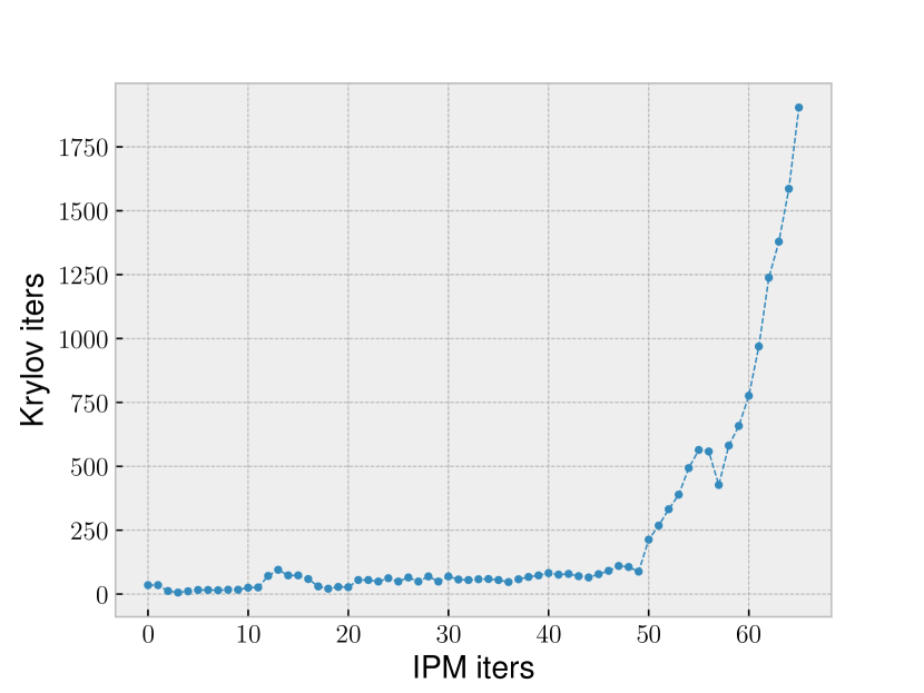
(a) VMAT Head and Neck case

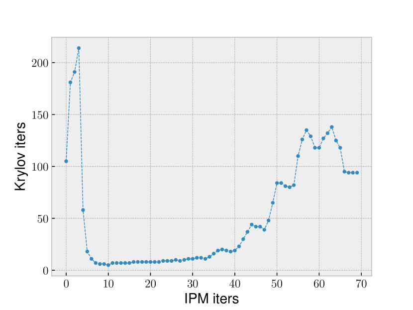
(b) Proton Head and Neck case

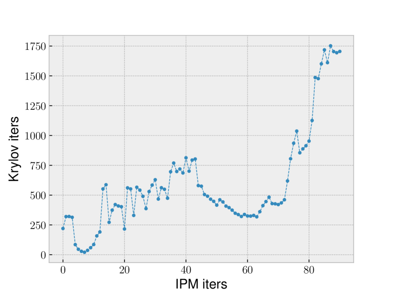
(c) Proton Liver Case

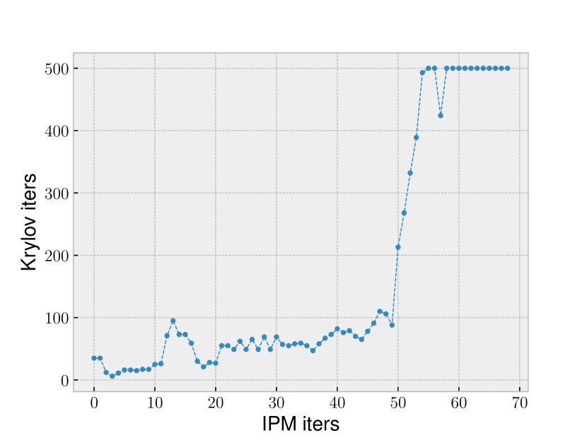
(d) VMAT Head and Neck case, 500 CG iterations max.

(e) Proton Head and Neck case, 500 CG iterations max.

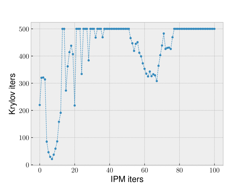
(f) Proton Liver Case, 500 CG iterations max.

Figure 1: Number of CG iterations at each IPM iteration for three different test problems. The bottom row shows the same problems with the maximum number of CG iterations set to 500.

In the following section, we present some experimental evaluation of our prototype method. In particular, we study the convergence of the preconditioned conjugate gradient method, the convergence of the interior point method, the conditioning of the KKT-systems, as well as the computational efficiency and some performance characteristics of our method. Ultimately, the goal is to understand how the ill-conditioning and characteristics of our particular types of problems affect the solver, and to assess the feasibility and promise in using Krylov solvers for interior point methods in this context.

5.1 Krylov Solver Convergence

Fig. 1 shows the number of CG iterations required for the linear solver to converge within each IPM iteration for our test problems. To study the effect of the accuracy and convergence of the CG solver on the optimization as a whole, we show two different setups. The top row in Fig. 1 shows the number of CG iterations to converge to a relative tolerance of $10^{-6}$, with no maximum number of CG iterations set. The second row shows the convergence when the number of CG iterations in each iteration of the interior point method was set to 500. The IPM solver converged to a value of $\mu=10^{-6}$ (see Algorithm 1) for all problems. For the VMAT Head and Neck case, the number of CG iterations increases sharply after iteration 50 in the interior point method. As discussed previously, we would expect the condition number of the KKT system to deteriorate as the barrier parameter $\mu$ approaches $0$. The proton head and neck case shown in Fig 1(b), which only has bound constraints on the variables, displays better convergence in the CG solver throughout the optimization. Finally, the proton liver case is the most challenging from the perspective of CG convergence.

The results with the maximum number of Krylov iterations set to 500 show a slight increase in the total number of IPM iterations required to reach convergence according to our criteria. For the VMAT Head and Neck case, the number of IPM iterations increased from 66 to 69, while for the proton liver case, the number of IPM iterations increased from 91 to 101. Overall, in relation to the total number of CG iterations for the entire optimization, the advantage in limiting the number of CG iterations is substantial. Previous work has also indicated that the use of a simple relative residual norm (on the form $||Ax-b||/||b||$), as we do in our implementation, to assess convergence of the Krylov sovler when used in IPMs may not be the most suitable, see [29]. In [29], the authors propose a different stopping criterion for the inner Krylov solvers, based on the residuals for the optimization problem instead. Overall, we conclude that there is a trade-off to be made with respect to the number of CG iterations used to find each search direction, and the total number of iterations of the interior point method required for convergence.

5.2 IPM Solver Convergence

(a) VMAT Head and Neck case

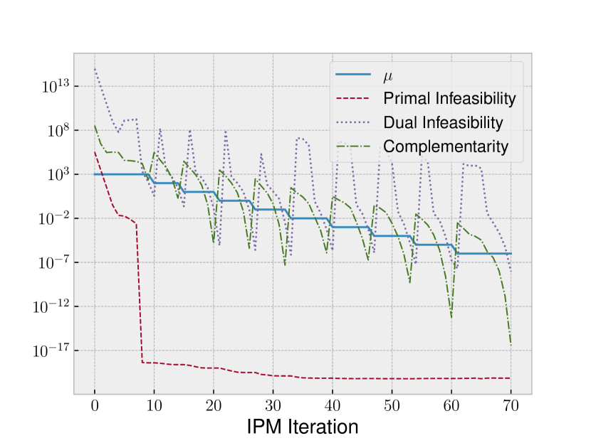
(b) Proton Head and Neck case

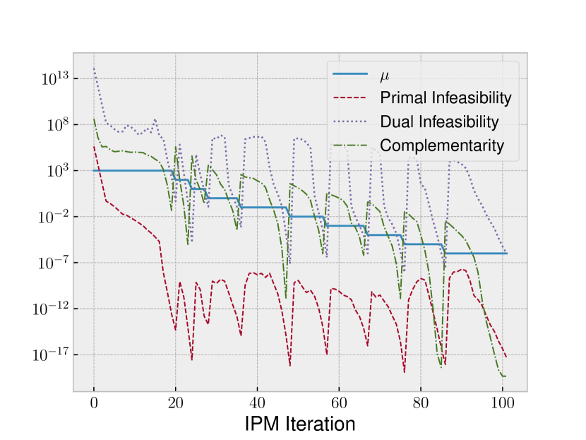
(c) Proton Liver Case

Figure 2: Convergence of our solver in terms of primal, dual and complementarity infeasibility. The value of the barrier parameter $\mu$ is shown as well, which is successively decreased as optimization progresses.

Another interesting aspect to consider is the convergence of the interior point method as a whole. In optimization solvers, the convergence is often measured with respect to the primal, dual and complementarity infeasibility (among others). The primal infeasibility is the (Euclidean) norm of

$$\begin{pmatrix}r_{l_{A}}&r_{u_{A}}&r_{l_{x}}&r_{u_{x}}\end{pmatrix}^{T},$$

the dual infeasibility is the norm of $r_{H}$ and the complementarity infeasibility the norm of

$$\begin{pmatrix}r_{c_{1}}&r_{c_{2}}&r_{c_{3}}&r_{c_{4}}\end{pmatrix}^{T}.$$

In other words, the primal infeasibility measures the error with respect to satisfying the constraints, the dual infeasibility measures the error in stationarity of the Lagrangian, and the complementarity infeasibility the error with respect to the perturbed complementary slackness condition.

In Fig 2, we show the convergence in terms of the primal, dual and complementarity infeasibility over IPM iterations for our test-problems. From the figures, we see that the convergence towards optimality is far from monotonous, with the spikes in the infeasibility norms coinciding with the points when the barrier parameter $\mu$ is decreased in the solver. This could indicate that the update of $\mu$ is too aggressive. The reason could be that we use a relatively crude update rule for $\mu$ in our prototype implementation, and more sophisticated methods may give better performance. Another interesting observation from the infeasibility plots is that the dual infeasibility exhibits slower convergence compared to the complementarity and primal infeasiblities, especially for the proton cases.

Speculatively, one can observe that the dual infeasibility $r_{H}$, appears only once in the right-hand side of (2.10). The block in the RHS in which the dual infeasibility appears is also contains multiple terms scaled by the inverse of the slack variables, which may be large for active constraints. The doubly augmented system (3.20) introduces an additional term in the top block of the RHS. In view of Krylov methods as algorithms seeking least-norm solutions in a given Krylov subspace for a set of linear system of equations, this may give a partial explanation why the dual infeasibility lags behind in our case, as the contribution to the RHS in the linear system from the corresponding term can be relatively small.

It bears reminding at this stage that our problems are QP subproblems from a sequential quadratic programming (SQP) algorithm for nonlinear optimization problems (as discussed in Section 2.3), which gives an additional level at which to consider the requirements on solution accuracy. Namely, the solution to the QP given by our interior point method is used as search direction for the SQP-solver, and there is naturally a trade-off between the accuracy of the solution to the QP-subproblem and the time required to solve the subproblem. Ultimately, we find this topic to be out of scope for this paper, but it remains an interesting consideration for future research.

5.3 Numerical Stability and Conditioning of KKT System

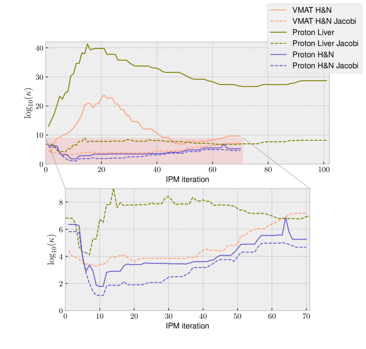
Figure 3: Condition number estimates using Matlab’s condest throughout the optimization iterations. The bottom plot is zoomed in on the red region (with the VMAT H&N line removed for clarity).

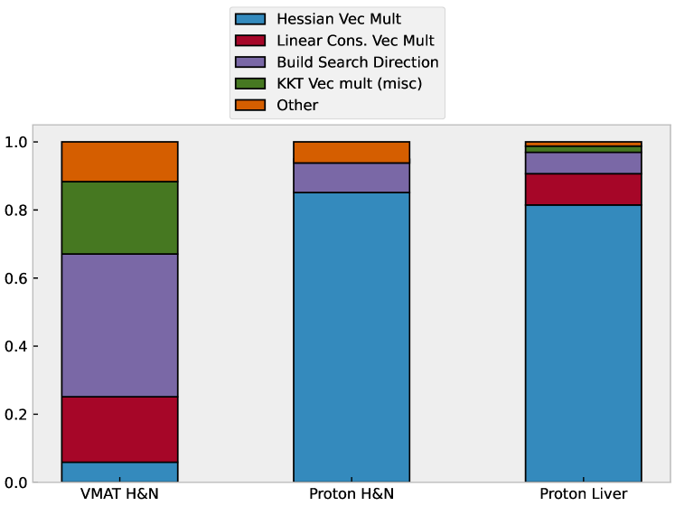
Figure 4: Relative (normalized) run-time spent in different computational kernels for our solver.

As discussed previously, one of the main challenges in using iterative linear solvers for interior point methods is the structured ill-conditioning in the linear systems. To study how this conditioning affects our problem, we evaluate how the condition number $\kappa$ of the doubly augmented KKT system (3.20) that we solve in each iteration changes throughout the optimization. Recall that the condition number measures the sensitivity of a function to errors in the input, with a larger value corresponding to greater sensitivity of the output to errors in the input value. We export the data from the solver required to build the matrix in (3.20) in each IPM iteration. The condition numbers of the resulting matrices are estimated using Matlab’s condest function, which we modify slightly by using Cholesky instead of LU-factorization internally, since our matrices are symmetric positive definite. condest gives an estimate of the condition number in the $L1$-norm and is based on an algorithm proposed by Higham in [15].

Figure 4 shows the results of the condition number analysis. The solid lines show the un-preconditioned condition numbers, with the dashed lines showing the condition numbers with Jacobi preconditioning. The un-preconditioned KKT systems for the VMAT H&N and Proton Liver cases show extreme ill-conditioning, especially in the middle of the optimization, with estimated condition numbers up to the order $10^{41}$ for the Proton Liver case and $10^{23}$ for the VMAT H&N case. While the accuracy of Matlab’s estimation using condest at such extreme ill-conditioning may be questioned, suffice it to say that the un-preconditioned matrices are close to singular. However, we see that the Jacobi preconditioning does manage to improve the conditioning of those matrices significantly, reducing the condition number to around $10^{8}$ (or less) for both cases.

Another interesting observation is that the number of CG iterations required for convergence (shown in Figure 1) at each step seem to, as a general trend, follow the conditioning of the matrices. For example, the preconditioned KKT matrix for the VMAT H&N case has a gradually rising condition number throughout with a sharper rise towards the end of the optimization, and the number of CG iterations (Figure 1(d)) also follows that trend. Similar patterns can be seen for the preconditioned Proton Liver case and Proton H&N case. This is perhaps unsurprising, but differs from the more benign effects of ill-conditioning when using direct solvers, as in [27, 10].

5.4 Performance Analysis

Case	Total	Hessian	Lin. Cons.	Build Search Dir.	KKT Misc.	Other
VMAT H&N	12.6	0.745	2.43	5.29	2.69	1.47
Proton H&N	12.3	10.4	0.0	1.20	0.0	0.759
Proton Liver	336	274	30.8	21.1	6.13	4.23

Table 2: Total run times in seconds spent in different parts of the solver for the different problems. The relative times in different parts are also visualized in Figure 4.

One of the motivations for moving towards iterative linear solvers in interior point methods is accelerators and GPUs. The key computational kernel in any Krylov method is the application of a linear operator on a vector (typically a matrix-vector product in practice), which is in many cases well suited for hardware accelerators. To empirically assess the suitability of our method for GPU acceleration, we performed tracing and profiling of our solver to see where time is spent.

Figure 4 shows the relative time spent in different parts of the code for the three test problems considered in this work. The absolute run-times for the different parts is given in Table 2. The parts we included in the profiling are: Matrix-vector multiplication with the quasi-Newton Hessian, matrix-vector multiplication with the constraint matrix, building the full search direction from equation (2.11), remaining time spent in the matrix-vector multiplication with the Doubly Augmented KKT system in (3.20), and finally the ”Other” category comprising the remaining time spent in other parts of the solver.

From Figure 4, we see that for both proton cases, the solver spends the majority of the time in computing matrix-vector products with the quasi-Newton Hessian. This is perhaps unsurprising considering the dimensions of the problems shown in Table 1. The proton cases are characterized by having a larger number of variables, with few or no general linear constraints, thereby placing the bulk of the computational burden on multiplications with the Hessian. For the VMAT case, the situation is different, with a smaller number of variables, but a significant number of general linear constraints. This difference is also clearly seen in the profiling, with only a small fraction of total time spent in quasi-Newton Hessian multiplication, and a significant portion of time spent in multiplications with the linear constraint matrix, as well as to assemble the final search direction.

As a preliminary observation, it seems that the different optimization problems arising from proton therapy are likely well suited to GPU acceleration. A majority ($>80\%$) of time in those cases is spent in multiplication with the quasi-Newton Hessian, which essentially comprises a series of dense matrix-vector multiplications, which is a computational kernel we expect to perform well on GPU. The VMAT case is more challenging from this perspective. To conclude, profiling suggests that GPU acceleration may benefit the different proton cases more than the VMAT case, mainly due to the structure of the arising optimization problems.

6 Related Work

The topic of iterative linear solvers in interior point methods has attracted much research, which we briefly summarize in the following section. Preconditioners for KKT systems in interior point method have been studied extensively previously, for instance in [1, 16, 12, 20, 5, 30] among many others. For a more complete overview of different research on the topic of preconditioning, we refer to [19] and the references therein. A general overview of HPC in the space of optimization and optimization software can be found in [17]. The topic of parallel computing in optimization and operations research in general has also been surveyed previously [23].

Practical studies where iterative linear solvers are used for different kinds of optimization problems can be found in [21], where a type of hybrid direct-iterative solution method is evaluated on very large problems in optimal power flow. In the context of interior point methods for linear programming (LP), preconditioned Krylov methods were studied in [5] on an extensive set of standard LP benchmarking problems. Other recent work on preconditioning for iterative methods for LP includes the work in [4], where preconditioners constructed using techniques from randomized linear algebra were considered.

7 Conclusions and Future Work

In this work, we have presented our prototype interior point method for quadratic programming that uses an iterative linear solver for the KKT systems arising in each iteration. We demonstrate that the method can solve real optimization problems from radiation therapy to acceptable levels of accuracy and within reasonable time. From analyzing the performance of our implementation using tracing and profiling, we believe that our method is suitable for GPU acceleration, which we will investigate further in future work. Overall, we believe that interior point methods using Krylov solvers give a promising path forward for porting more parts of the computational workflow in radiation therapy treatment planning to GPU accelerators.

While we believe this initial study on the use of iterative linear solvers for optimization of radiation therapy treatment plans shows promise, there are many interesting questions and problems remaining for future research. Among those is the porting of the code to be able to run on GPU accelerators, looking at improved preconditioners for the KKT systems and investigating the applicability of the method to optimization problems from other domains.

From the perspective of applying the method to optimization problems from other areas, one aspect missing from our solver is the ability to handle equality constraints. A challenge in many formulations of the KKT systems with equality constraints is that one may end up with a matrix with a zero-block on the diagonal, see e.g. [14]. This, at the very least, presents a challenge for our diagonal scaling preconditioning. Adding a small regularization term to the diagonal could alleviate the issue, or one might consider handling equality constraints another way, for instance by a quadratic penalty term in the objective, as discussed in [11]. Evaluating which approach is most suitable could be an interesting direction for future studies.

Improved preconditioners is another interesting topic, especially for problems with general linear constraints (and not only bound constraints on the variables). A key challenge in defining those lies in striking a balance between the cost of applying the preconditioner and the improvement in convergence of the linear solver. An example on one extreme could be a preconditioner that requires the factorization of a matrix similar in size to the problem matrix may be too expensive. On the other hand, the Jacobi preconditioner used in this work may be too simple, as seen in the sometimes large number of Krylov iterations required. Many preconditioning techniques have been described in the literature, though evaluating their suitability to different types of optimization problems and formulations remains a substantial task.

8 Acknowledgment

The computations were enabled by resources provided by the National Academic Infrastructure for Supercomputing in Sweden (NAISS) at PDC, partially funded by the Swedish Research Council through grant agreement no. 2022-06725.

References

- [1] Luca Bergamaschi, Jacek Gondzio, and Giovanni Zilli. Preconditioning indefinite systems in interior point methods for optimization. Computational Optimization and Applications, 28:149–171, 2004.
- [2] Charles George Broyden. The convergence of a class of double-rank minimization algorithms 1. general considerations. IMA Journal of Applied Mathematics, 6(1):76–90, 1970.
- [3] Joo-Siong Chai and Kim-Chuan Toh. Preconditioning and iterative solution of symmetric indefinite linear systems arising from interior point methods for linear programming. Computational Optimization and Applications, 36:221–247, 2007.
- [4] Agniva Chowdhury, Gregory Dexter, Palma London, Haim Avron, and Petros Drineas. Faster randomized interior point methods for tall/wide linear programs. Journal of Machine Learning Research, 23(336):1–48, 2022.
- [5] Yiran Cui, Keiichi Morikuni, Takashi Tsuchiya, and Ken Hayami. Implementation of interior-point methods for lp based on krylov subspace iterative solvers with inner-iteration preconditioning. Computational optimization and applications, 74:143–176, 2019.
- [6] Matthias Ehrgott, Çiğdem Güler, Horst W Hamacher, and Lizhen Shao. Mathematical optimization in intensity modulated radiation therapy. Annals of Operations Research, 175(1):309–365, 2010.
- [7] Lovisa Engberg. Automated radiation therapy treatment planning by increased accuracy of optimization tools. PhD thesis, KTH Royal Institute of Technology, 2018.
- [8] Roger Fletcher. A new approach to variable metric algorithms. The computer journal, 13(3):317–322, 1970.
- [9] Anders Forsgren, Philip E Gill, and Joshua D Griffin. Iterative solution of augmented systems arising in interior methods. SIAM Journal on Optimization, 18(2):666–690, 2007.
- [10] Anders Forsgren, Philip E Gill, and Joseph R Shinnerl. Stability of symmetric ill-conditioned systems arising in interior methods for constrained optimization. SIAM Journal on Matrix Analysis and Applications, 17(1):187–211, 1996.
- [11] Anders Forsgren, Philip E Gill, and Margaret H Wright. Interior methods for nonlinear optimization. SIAM review, 44(4):525–597, 2002.
- [12] Philip E Gill, Walter Murray, Dulce B Ponceleón, and Michael A Saunders. Preconditioners for indefinite systems arising in optimization. SIAM journal on matrix analysis and applications, 13(1):292–311, 1992.
- [13] Donald Goldfarb. A family of variable-metric methods derived by variational means. Mathematics of computation, 24(109):23–26, 1970.
- [14] Jacek Gondzio. Interior point methods 25 years later. European Journal of Operational Research, 218(3):587–601, 2012.
- [15] Nicholas J Higham. Fortran codes for estimating the one-norm of a real or complex matrix, with applications to condition estimation. ACM Transactions on Mathematical Software (TOMS), 14(4):381–396, 1988.
- [16] Samah Karim and Edgar Solomonik. Efficient preconditioners for interior point methods via a new schur complement-based strategy. SIAM Journal on Matrix Analysis and Applications, 43(4):1680–1711, 2022.
- [17] Felix Liu, Albin Fredriksson, and Stefano Markidis. A survey of hpc algorithms and frameworks for large-scale gradient-based nonlinear optimization. The Journal of Supercomputing, 78(16):17513–17542, 2022.
- [18] Karl Otto. Volumetric modulated arc therapy: Imrt in a single gantry arc. Medical physics, 35(1):310–317, 2008.
- [19] John W Pearson and Jennifer Pestana. Preconditioners for krylov subspace methods: An overview. GAMM-Mitteilungen, 43(4):e202000015, 2020.
- [20] Tim Rees and Chen Greif. A preconditioner for linear systems arising from interior point optimization methods. SIAM Journal on Scientific Computing, 29(5):1992–2007, 2007.
- [21] Shaked Regev, Nai-Yuan Chiang, Eric Darve, Cosmin G Petra, Michael A Saunders, Kasia Świrydowicz, and Slaven Peleš. Hykkt: a hybrid direct-iterative method for solving kkt linear systems. Optimization Methods and Software, pages 1–24, 2022.
- [22] Yousef Saad. Iterative methods for sparse linear systems. SIAM, 2003.
- [23] Guido Schryen. Parallel computational optimization in operations research: A new integrative framework, literature review and research directions. European Journal of Operational Research, 287(1):1–18, 2020.
- [24] David F Shanno. Conditioning of quasi-newton methods for function minimization. Mathematics of computation, 24(111):647–656, 1970.
- [25] Kasia Świrydowicz, Eric Darve, Wesley Jones, Jonathan Maack, Shaked Regev, Michael A Saunders, Stephen J Thomas, and Slaven Peleš. Linear solvers for power grid optimization problems: A review of gpu-accelerated linear solvers. Parallel Computing, 111:102870, 2022.
- [26] Margaret H Wright. Interior methods for constrained optimization. Acta numerica, 1:341–407, 1992.
- [27] Margaret H Wright. Ill-conditioning and computational error in interior methods for nonlinear programming. SIAM Journal on Optimization, 9(1):84–111, 1998.
- [28] Stephen Wright. Stability of augmented system factorizations in interior-point methods. SIAM Journal on Matrix Analysis and Applications, 18(1):191–222, 1997.
- [29] Filippo Zanetti and Jacek Gondzio. A new stopping criterion for krylov solvers applied in interior point methods. SIAM Journal on Scientific Computing, 45(2):A703–A728, 2023.
- [30] Giovanni Zilli and Luca Bergamaschi. Block preconditioners for linear systems in interior point methods for convex constrained optimization. ANNALI DELL’UNIVERSITA’DI FERRARA, 68(2):337–368, 2022.