Spread complexity evolution in quenched interacting quantum systems

Abstract

We analyse time evolution of spread complexity (SC) in an isolated interacting quantum many-body system when it is subjected to a sudden quench. The differences in characteristics of the time evolution of the SC for different time scales is analysed, both in integrable and chaotic models. For a short time after the quench, the SC shows universal quadratic growth, irrespective of the initial state or the nature of the Hamiltonian, with the time scale of this growth being determined by the local density of states. The characteristics of the SC in the next phase depend upon the nature of the system, and we show that depending upon whether the survival probability of an initial state is Gaussian or exponential, the SC can continue to grow quadratically, or it can show linear growth. To understand the behaviour of the SC at late times, we consider sudden quenches in two models, a full random matrix in the Gaussian orthogonal ensemble, and a spin-$1/2$ system with disorder. We observe that for the full random matrix model and the chaotic phase of the spin-$1/2$ system, the complexity shows linear growth at early times and saturation at late times. The full random matrix case shows a peak in the intermediate time region, whereas this feature is less prominent in the spin-$1/2$ system, as we explain.

I Introduction

The concept of complexity in the context of a quantum mechanical state refers to how ‘difficult’ it is to construct the desired state via some pre-assigned basis states and operators. Even though it is a widely used measure in quantum computation research, the recent flurry of activity in quantum field theory and statistical systems started after the work of Jefferson:2017sdb , where a proposal for circuit complexity of a quantum state was described, based on Nielsen’s geometric approach to the circuit complexity Nielsen1 ; Nielsen2 ; Nielsen3 . The Nielsen complexity and various other related notions of complexity of a quantum state under a unitary evolution was proposed and studied subsequently in several works Khan:2018rzm ; Hackl:2018ptj ; Bhattacharyya:2018bbv (see the review Chapman:2021jbh for a compendium of related works).

Besides these measures of circuit complexity, in a slightly different context of probing operator growth in quantum-many body systems, the notion of Krylov complexity (KC) was proposed in Parker:2018yvk . The central result of this work was embodied in the ‘universal operator growth’ hypothesis, which states that for a non-integrable quantum many-body system in the thermodynamic limit, the so-called Lanczos coefficients must grow linearly with $n$ (with logarithmic corrections present for one dimensional systems, where $n$ denotes the index of the ordered Krylov basis). This implies that the corresponding operator complexity must grow exponentially fast, a feature quite generic in quantum chaotic systems. Since then, KC has become a popular measure to study various aspects of quantum many-body dynamics in and out of equilibrium. For a partial set of works see Barbon:2019wsy ; Bhattacharjee:2022vlt for the use of Krylov complexity in operator growth, Dymarsky:2019elm ; Dymarsky:2021bjq ; Kundu:2023hbk for works in CFTs, Bhattacharya:2022gbz ; Bhattacharjee:2022lzy ; Bhattacharya:2023zqt for works on open systems, Bhattacharyya:2023dhp for KC in Bosonic systems, Kim:2021okd as a tool of probing delocalization properties in integrable quantum systems, Hashimoto:2023swv ; Camargo:2023eev focuses on billiard systems. Important steps has also been taken to understand features of KC in QFTs Avdoshkin:2022xuw ; Camargo:2022rnt . Various other important results have also been reported in Yates:2021asz - Erdmenger:2023shk .

From a viewpoint more in line with the Nielsen-like complexities, where the complexity is defined as the minimum of a ‘cost-functional’ associated with the evolution, the idea of spread complexity (SC) was proposed in Balasubramanian:2022tpr . In that work, it was shown that the cost that measures the spread of a reference wave function in a fixed basis of states on the Hilbert space under a unitary Hamiltonian evolution is the minimum when computed with respect to the Krylov basis constructed by using the Hermitian operator generating the evolution. The associated complexity, the SC, is the analogue of the operator complexity for quantum states. Starting from the work of Balasubramanian:2022tpr , the generic features of SC in quantum systems have been explored in a variety of works that includes quantum phase transition Caputa2 ; Caputa:2022yju ; spread1 , work statistics in quantum quench Pal:2023yik ; Gautam:2023pny , probing quantum scar states Nandy:2023brt among others. In this paper our main focus will be SC evolution in quantum many-body systems which are far away from equilibrium.

We note that the evolution of various few-body observables has been studied in the literature, specifically due to their importance in quench experiments. However, studies on the quench dynamics of the SC have been relatively rare, and these have been mostly confined to Hamiltonians that can be transformed to integrable systems Caputa2 , spread1 (there are various works that have studied the evolution of other measures of complexities after a quantum quench, see, e.g., Alves - Pal:2022rqq ). In this context, the importance of introducing interactions in an otherwise isolated quantum system cannot be over-emphasized, since integrable systems constitute a small subset of realistic quantum systems with interactions. With this motivation, in this work, we go beyond the realm of integrable models, and understand the evolution of SC after a sudden quantum quench is performed in generic interacting many-body quantum systems. Here, we highlight the differences in the characteristics of the time evolution shown by the SC for different time scales after the quench, both in integrable and chaotic models. It is known that the exact nature of the dynamics of an interacting quantum system after a sudden quantum quench depends on how the local density of states (LDOS) is filled up after the quench. Therefore, the spread of an initial state before the quench in the Krylov basis, and hence the SC should crucially depend on how the LDOS behave in that interacting system. Our aim in this paper is to find out this connection. We shall highlight how the filling of the LDOS affect the evolution of the SC after the quench.

To begin with, the basic approach of obtaining the Lanczos coefficients (LCs) and the associated SC after a sudden quantum quench used in this paper is the following. We recall that all information about the LCs, which are the main ingredients of constructing the Krylov basis by means of the Lanczos algorithm Viswanath ; Lanczos:1950zz ; Parker:2018yvk ; Balasubramanian:2022tpr , are encoded in the moments of the so called auto-correlation function, which measures the overlap between the evolved quantum state with the initial one. Once this is known, the full set of Krylov basis can be constructed from the moments of the auto-correlation function at $t=0$, where $t$ denotes the time after the quench Viswanath . Typically, for the Hamiltonian evolution, there are two sets of LC, which are denoted by $a_{n}$ and $b_{n}$. The first set of coefficients give the expectation value of the Hamiltonian in each Krylov basis, and the second set represents the normalization constants for these bases. Therefore, we can extract all the relevant information about the dynamics in Krylov space, and the time evolution of SC, once we have an analytical (or numerical) expression for the auto-correlation function in hand. In this context, we note that the characteristic function (CF, which is just the complex conjugate of the auto-correlation function) is one one of the most commonly studied quantities in sudden quenches of interacting quantum many-body system and by itself can reveal important information about the nature of the post-quench Hamiltonian and the initial state before the quench. For example, usually when the CF after a quench decays exponentially, it means that the post-quench Hamiltonian is chaotic in nature Peres ; Cerrtui , however, whenever the initial state is ‘sufficiently delocalised’ in the energy basis, similar exponential decay can also be observed in integrable systems Emerson .

With this discussion in mind, in this work we first explore in detail the evolution of SC in generic interacting lattice quantum-many body systems, where the analytical form of the auto-correlation functions are known in the literature for a wide range of such systems at different time scales after a sudden quench. In many cases approximate analytical expressions for such auto-correlation functions have been obtained by comparing with results from numerical simulations. In this work we use these generic expressions for such auto-correlation functions to obtain the nature of SC evolution for a wide class of realistic interacting quantum many-body systems after a sudden quench.

In the next section, first we use the expression for the survival probability (SP) of an initial state before the quench, available in the literature for sudden quantum quenches of a parameter of the Hamiltonian of a generic quantum system, to comment on the universal features of SC. We find that the SC shows quadratic growth at early times, where the rate of the growth is set by the variance of the local density of states, or equivalently, the LC $b_{1}$. It is to be noted that, the quadratic early time behaviour of SC was also reported in Balasubramanian:2022tpr for evolution with random matrices. Our result points toward the universality of this feature in an interacting quantum many-body system. However, our results also suggest that, besides this universal early time quadratic growth, this type of growth can persist for even larger times scales in quenches of quantum many-body systems where the interaction is strong. Next, to explore the behaviour of complexity at late times, we use an interpolating functional form of the SP that incorporates between the quadratic decay at early times and exponential decays at late times, valid when the external perturbation is not strong, to show that in such a case the LCs $b_{n}$ follow a liner growth for relatively small values of $n$ (which determine the early time evolution of the complexity) and the SC, after the initial universal quadratic growth, merges into a linear growth at late times.

In the rest of section III, we briefly describe the results for LCs and the SC evolution when one uses a full random matrix (FRM) to describe the Hamiltonian of the interacting quantum many-body system after quantum quench by sampling its elements from a Gaussian orthogonal ensemble (GOE). Here, we use the tri-diagonal Hessenberg form of the Hamiltonian to extract the corresponding LCs and later use this form to find the nature of the SC at various time scales. In this context, we note that, in the original work, which introduced the notion of SC Balasubramanian:2022tpr , the evolution of the SC was explored in detail for quantum chaotic systems modeled by random matrices. It was established that the SC shows a characteristic structure - linear ramp, peak, slope and plateau around a constant value. These characteristics were further studied in Erdmenger:2023shk , where it was shown that the late-time features of SC are determined by the probability amplitude of each Krylov basis, and is a universal indicator of quantum chaos. In this work we use an analytical form for the auto-correlation function after a sudden quench (obtained in Herrera9 ) to find out an approximate shape of the distribution of $b_{n}$s.

In section IV, we consider a more realistic model of an interacting quantum many-body system, i.e., an interacting spin-$1/2$ model with disorder. With increasing disorder, the system transforms from an integrable to non-integrable phase, and finally to an intermediate limit between the chaotic phase and the many-body localised phase for large disorder values. Using a phenomenological expression for the SP after a sudden quench, we obtain both sets of LCs and hence the SC when the system is in chaotic domain, as well as in the intermediate phase. Our observations show that in the non-integrable phase, the SC shows linear growth at early times and saturation at late times, however, the peak in the complexity, present in the FRM case, is less pronounced here. The implications of these results and conclusions are discussed in section V. This paper also contains an Appendix where we briefly review the construction of the Krylov basis and the definition of the SC.

II Auto-correlation function and survival probability after a sudden quantum quench

We assume that a quantum many-body system with an initial Hamiltonian $H_{0}$ and prepared in the ground state $\big{|}\psi_{0}\big{>}$ is quenched at time $t=0$ to a new Hamiltonian $H$, whose eigenvalues and eigenfunctions are denoted by $E_{n}$ and $\big{|}n\big{>}$, respectively. To find out the behaviour of the time evolution of the SC, we need to study time scales associated with the CF, which in this case is given by

$$\mathcal{G}(t)=\big{<}\psi_{0}\big{|}\Psi(t)\big{>}=\sum_{n}\big{|}C_{0}^{n}\big{|}^{2}e^{-iE_{n}t}~{},$$ (1)

where $C_{0}^{n}=\big{<}n\big{|}\psi(0)\big{>}$ represents the overlap between the initial state and the eigenstates of the post-quench Hamiltonian ($\big{|}n\big{>}$). As mentioned in the introduction, the auto-correlation function $\mathcal{S}(t)=\mathcal{G}^{*}(t)$. By introducing the LDOS

$$\rho_{0}(E)=\sum_{n}\big{|}C_{0}^{n}\big{|}^{2}\delta(E-E_{n})~{},$$ (2)

we can write down the CF as the Fourier transform of the LDOS, i.e.

$$\mathcal{G}(t)=\int dE\rho_{0}(E)e^{-iEt}~{}.$$ (3)

Therefore, once the LDOS is known for an initial state before the quench and the final Hamiltonian, the behaviour of the CF, and hence the auto-correlation function is completely fixed. Here we also note that for a given final Hamiltonian, the time evolution of the CF can be different for different choices of the location of the initial state in the energy spectrum of the initial Hamiltonian.

Detailed studies of the survival probability $F(t)$ (which is just the modulus squared of the auto-correlation $F(t)=\big{|}\mathcal{G}(t)\big{|}^{2}$, i.e. the fidelity) under quenches in integrable and chaotic quantum many-body systems have been carried out in a series of works herrera1 ; herrera2 ; herrera3 ; Santos1 ; Tavora1 . Here we briefly describe the behaviour of the SP for different time scales after the quench, following the above mentioned references.

For a very short time after the quench, the SP shows a universal quadratic decay, independent of the final Hamiltonian or the initial state before the quench. To check this, we first notice that the mean and the variance of the LDOS are given, respectively, by

$$E_{0}=\sum_{n}\big{|}C_{0}^{n}\big{|}^{2}E_{n}~{},~{}~{}~{}\text{and}~{}~{}\sigma_{0}^{2}=\sum_{n}\big{|}C_{0}^{n}\big{|}^{2}\big{(}E_{n}-E_{0}\big{)}^{2}=b_{1}^{2}~{},$$ (4)

where in the second expression we have used an identification between the variance of the LDOS and the LC $b_{1}$ Pal:2023yik . These two quantities are extremely important in determining the nature of the subsequent dynamics after a quench. Now expanding the expression for the SP, it is easy to see that, for small times $t\ll\sigma_{0}^{-1}$, it behaves as Tavora1 ; Santos1

$$F(t)\approx 1-\sigma_{0}^{2}t^{2}=1-b_{1}^{2}t^{2}~{}.$$ (5)

After this initial quadratic decay, the behaviour of the SP depends on the strength of the external perturbation (see below). For example, in systems with two-body interactions, the shape of the LDOS, as well as the density of states (DOS) is Gaussian, so that the resulting shape of the SP is given by the Gaussian function of the form $F(t)=\exp(-\sigma_{0}t^{2})$ Flambaum ; Izrailev ; herrera1 , and this decay can go up to a saturation. Furthermore, the LDOS can also be of the Lorentzian shape, so that the SP decays exponentially with time. These behaviour usually hold upto a time scale of $\sigma_{0}^{-1}\lesssim t\lesssim t_{P}$, where $t_{P}$ indicates the time scale where the decay of the SP follows a power law.

At late times therefore, the SP attains a power law decay of the form $F(t)\propto t^{-\gamma}$, where, the exact value of the exponent $\gamma$ crucially depends on the nature of the system under consideration, i.e. how the LDOS fills up, as well as the initial state before the quench. A detailed study of this power law decay and calculation of the resulting exponent has been performed in Tavora1 , where it was shown that from the numerical value of $\gamma$, we can predict whether a given initial state will thermalise or not, therefore providing a way to probe the thermalisation of an initial state based only on the dynamics after quench. It is thus clear that the exact nature of the dynamics of the SC will therefore depend on how the LDOS is filled, in the system under consideration. In this paper, our broad goal is to perform such analysis about the evolution of SC depending upon the different types of LDOS filling after the quench.

III Behaviour of spread complexity at early times after a sudden quench

Before considering quench dynamics in some specific models, here we first study the approximate evolution of the SC at different time scales after the quench, and the behaviour of the resulting LC using the evolution of the SP as described above. We assume that the Hamiltonian of the quantum system under consideration can be written as $H=H_{0}+gV$, where $H_{0}$ is the unperturbed Hamiltonian, and $V$ is an external perturbation, and $g$ denotes the strength of the external perturbation. We also assume that the state $\big{|}\psi_{0}\big{>}$ of the system before the quench is the first state of the Krylov basis i.e., $\big{|}K_{0}\big{>}=\big{|}\psi_{0}\big{>}$. The construction of the Krylov basis and the definition of the SC are briefly described in Appendix A. All other relevant details, which have been used in our numerical analysis below, can be found in Viswanath ; Lanczos:1950zz ; Balasubramanian:2022tpr .

III.1 Analysis for Gaussian exponential decays

First we consider the time scale $t\ll\sigma_{0}^{-1}$, where, as we have discussed above, the SP decays quadratically with time irrespective of the nature of the system under consideration or the initial state before the quench. Since before the quench, the state of the system is the lowest state of the Krylov basis, for times scales $t\ll\sigma_{0}^{-1}$ just after the quench, the time evolved state $\big{|}\Psi(t)\big{>}$ will spread over only the first few Krylov basis elements with small basis number $n$. Now we can use the auto-correlation function of the form $\mathcal{S}(t)=1-\frac{1}{2}\sigma_{0}^{2}t^{2}$ to obtain the first few LCs as well the SC. It can be checked that for this auto-correlation function, $a_{n}=0$, while $b_{n}$s grow with $n$ and are proportional to the width $\sigma_{0}$ of the LDOS. In Fig. 1, we have provided the numerical values of the first few $b_{n}$s with $\sigma_{0}=1$.

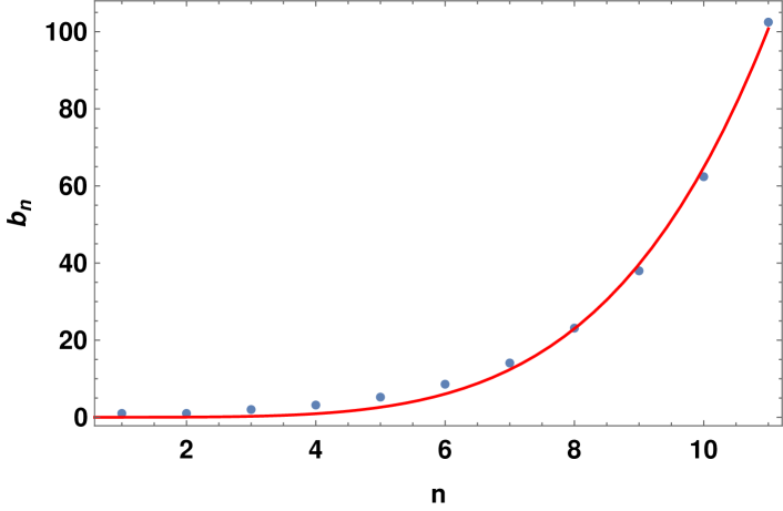
Figure 1: Numerical values of the first few $b_{n}$s. Here we have set $\sigma_{0}=1$, and $b_{n}$s are proportional to $\sqrt{\sigma_{0}}$. The red curve is of the form $n_{1}n^{n_{2}}$, and provides a good fit of the $b_{n}$s with $n_{1}\approx 0.0014$ and $n_{2}\approx 4.6446$.

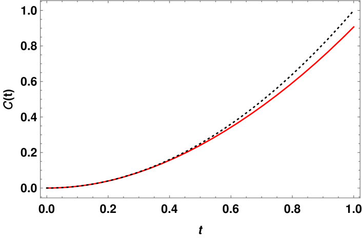
Figure 2: Time evolution of SC (red curve) for $t\ll\sigma_{0}^{-1}$ after the quench. Here we have set $\sigma_{0}=b_{1}=1$. The dotted black curve is the plot of $t^{2}$, which have a reasonably accurate matching with complexity at early times.

The time evolution of the SC for this case is shown in Fig. 2. Along with the complexity, calculated numerically (the red curve), we have also shown the plot of $t^{2}$, which reasonably approximates the SC curve at early times. Since the quadratic decay of the SP after quench is universal, we conclude that irrespective of the nature of the quantum many-body system under consideration, and the initial state before the quench, the SC will always grow quadratically, with the coefficient of the growth being determined by the variance of the LDOS, or equivalently, the LC $b_{1}$.

As we have discussed in the Introduction, after this initial quadratic decay, the nature of the time evolution of the SP and the auto-correlation function will depend on the exact nature of the quantum system under consideration. Two of the most common types of time evolutions encountered in the literature for quenches in interacting many-body quantum systems are the Gaussian and the exponential decays. These two types of decays appear in a chaotic system precisely when the shape of the LDOS is Gaussian and a Breit-Wigner form, respectively.

In the presence of strong interactions, the shape of the LDOS is Gaussian, so that the SP can be a function of the variable $\sigma_{0}^{2}t^{2}$ for a time scale much longer than $t_{0}<<\sigma_{0}^{-1}$ Flambaum2 , and the auto-correlation function (obtained from Eq. (1)) is of the form $S(t)\approx\exp\big{(}-\frac{\sigma_{0}^{2}}{2}t^{2}\big{)}$. For such a Gaussian form for the auto-correlation, the behaviour for the LC and the SC are well known, see e.g., Caputa1 ; Balasubramanian:2022tpr . Here the LCs are given by $a_{n}=0$, and $b_{n}=\sigma_{0}\sqrt{n}$, and the resultant SC grows quadratically with time, with the coefficient of this growth being determined by the variance $\sigma_{0}$ of the LDOS. Therefore, in the presence of strong interactions, the initial quadratic growth of the SC persists for time scales longer than $t_{0}(\ll\sigma_{0}^{-1})$.

In many cases, even in the presence of Gaussian LDOS, an initial Gaussian decay can change to an exponential decay before reaching saturation Flambaum ; Flambaum2 (see below for dynamics of the SC in such cases). However, the Gaussian decay can also persist until saturation. This was indeed shown to be the case for sudden quenches in XX model, and spin-$1/2$ systems with impurities in Herrera7 . Therefore, for quenches in these systems, the characteristic quadratic growth of the SC continues upto the saturation point of the SP.

For perturbations that are not very strong ($g<1$), the long time decay of the SP is exponential, and hence it can be written as $F(t)\approx\exp\big{(}-\Gamma t\big{)}$, where $\Gamma$ is the width of the corresponding Breit-Wigner distribution of the LDOS. In this case, it is interesting to consider an extrapolation formula for the SP derived in Flambaum2 , which interpolates between the initial quadratic and the long time exponential decays. The proposed form for the CF can be written as

$$\mathcal{G}(t)=\exp\Bigg{[}\frac{\Gamma^{2}}{4\sigma_{0}^{2}}-\frac{1}{2}\sqrt{\frac{\Gamma^{4}}{4\sigma_{0}^{4}}+\Gamma^{2}t^{2}}\Bigg{]}~{}.$$ (6)

It can be easily checked from this expression that for $\Gamma<\sigma_{0}$, this functional form for the CF represents the initial quadratic decay of the form in Eq. (5), while at late times it gives rise to $F(t)\approx\exp\big{(}-\Gamma t\big{)}$. Furthermore, we also note that for this form for the SP, the width (i.e. the second moment) of the corresponding LDOS is not $\sigma_{0}$. We use this CF to calculate the LC and the time dependence of the SC.

The first set of LC $a_{n}$ calculated from the CF in Eq. (6) are zero in this case as well, while the first few $b_{n}$s are shown in Fig. 3 for two different values of the variance of the LDOS. As can be seen in both cases, these $b_{n}$s evaluated numerically can be fitted with curves of the form $b_{n}=n_{1}n^{n_{2}}$, where the exponent $n_{2}$ is approximately equal to unity in both the cases, i.e. $b_{n}\approx n_{1}n$. The slope of the straight line fitting depends on the variance $\sigma_{0}$ in such a way that higher the variance, the higher is the slope of the straight-line fitting. For example, for the red dots with $\sigma_{0}=2$ we find $n_{1}=21.687$, and for the blue dots, plotted with $\sigma_{0}=1.2$ we obtain $n_{1}=7.682$. Therefore, for systems with LDOS of same shape but different widths, the growth rate of $b_{n}$s is higher when width of the LDOS is greater, which in turn results in faster decay of the SP.

Figure 3: Numerical values of the first few $b_{n}$s calculated from the CF in Eq. (6). The red dots are with $\sigma_{0}=2$, and blue dots are with $\sigma_{0}=1.2$, where in both the cases $\Gamma$ is fixed to $0.5$. The straight lines show the linear fitting to the numerically evaluated $b_{n}$s.

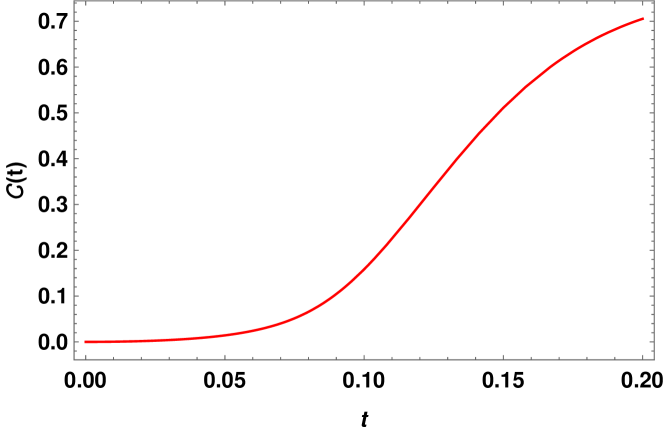
Figure 4: Time evolution of SC with $\sigma_{0}=2$ and $\Gamma=0.5$ (red dots in Fig. 4). The initial quadratic growth transforms to a linear growth at late times, with the time scale of the transformation being determined by the variance of the LDOS.

The time evolution of the SC (with values of $\sigma_{0}=2$ and $\Gamma=0.5$, for the red dots in Fig. 3) is shown in Fig. 4. For other values of the parameters, the features shown by the time evolution of the SC are similar. As can be seen, the initial quadratic growth of the SC (valid for the time scale $t\ll\sigma_{0}^{-1}$) transforms to an approximately linear growth at late times.

Since the variance of the LDOS $\sigma_{0}$ is the quantity which sets the time scale of the initial quadratic growth, the time where the quadratic growth matches with the linear growth occurs at a later time in the second case (blue dots) considered in Fig. 3, than the one first case (red dots). Therefore, when $\sigma_{0}^{-1}=1.2$, the quadratic growth of the SC persists for a longer amount of time, than when $\sigma_{0}^{-1}=2$. In the opposite case, where we fix the variance of the LDOS, and change $\Gamma$, the higher value of $\Gamma$ leads to lower values of the slope of the linear fit for the $b_{n}$s. This observation clearly illustrate the role of the initial state before the quench on the growth rate of the corresponding LCs, and hence the SC.

III.2 Analysis with full random matrices

After finding out the behaviour of the SC at time scales just after the quench ($t_{0}<<\sigma_{0}^{-1}$), and in intermediate times before the power law of the SP sets up for a wide class of generic interacting quantum many-body system, in this section we consider evolution of SC late times after quench. First we consider time evolution when the post-quench Hamiltonian is modeled by full random matrices.

Indeed, one of the most common approaches used to study a strongly chaotic quantum system is to model them as full random matrices (FRM). A quantum chaotic system usually shows Wigner-Dyson distribution of the spacings of neighboring energy levels due to the presence of strong level repulsion Mehta ; Guhrrev . In this subsection, we assume the quenched Hamiltonian to be a FRM from the Gaussian orthogonal ensembles (GOE), so that it is actually possible to obtain an analytical expression for the SP and hence the CF Santos1 . Modeling a quantum many-body system as a FRM is clearly not a realistic choice, since it implies simultaneous as well as infinite-range interactions between all the particles of the system. However, in this case, we can use the analytical formula for the CF to gain insights into the nature of the LC and the complexity evolution after quench to apply these in a more realistic model considered in the next section.

In this context, we mention that the LC and the SC in evolution with random matrices (RM) have been studied in details in Balasubramanian:2022tpr , where universal characteristics of the SC evolution for such RM models were established. In this section, our main goal is to use the analytical expression for the SP obtained when FRM is used to model the Hamiltonian after a quench Santos1 ; Herrera4 , and to understand the effect of two-level form factor (which is non-vanishing only in systems that have correlations between energy levels) in the expressions for the LC and the time evolution of the SC.

As before, we assume that the Hamiltonian after a quench is given by $H=H_{0}+V$, where $H_{0}$ is the unperturbed Hamiltonian, and $V$ is an external perturbation, i.e., by quenching we give a non-zero value to it. When we use the FRM, the matrix elements of the Hamiltonian $H_{nm}$ are random numbers, and since we are considering the GOE, these numbers are taken from a Gaussian distribution with a mean value of zero. The expression for the SP for a quenched quantum system modeled by FRM belonging to the GOE can be written as Herrera9 ; Santos1

$$\big{<}F(t)\big{>}_{FRM}=\frac{1-\big{<}\bar{F}\big{>}_{FRM}}{\mathcal{N}-1}\bigg{[}4\mathcal{N}\frac{J_{1}^{2}(\eta t)}{(\eta t)^{2}}-\mathcal{B}_{2}\Big{(}\frac{\eta t}{4\mathcal{N}}\Big{)}\bigg{]}+\big{<}\bar{F}\big{>}_{FRM}~{}.$$ (7)

Here, $\big{<}.\big{>}_{FRM}$ denotes the ensemble average, $\mathcal{N}$ is the size of the RM under consideration, $\eta=\sqrt{2\mathcal{N}}$ and $J_{1}(t)$ is the Bessel function of the first kind. Furthermore, $\bar{F}=\sum_{n}\big{|}C_{0}^{n}\big{|}^{4}$, so that for GOE FRM we have $\big{<}\bar{F}\big{>}_{FRM}=3/(\mathcal{N}+2)$. The functional form for the time dependence of the function $\mathcal{B}_{2}(t)$, known as the two-level form factor is given by Herrera9 ; Santos1

$$\mathcal{B}_{2}(t)=\Big{[}1-2t+t\ln(1+2t)\Big{]}\Theta(1-t)+\Big{[}t\ln\Big{(}\frac{2t+1}{2t-1}\Big{)}-1\Big{]}\Theta(t-1)~{},$$ (8)

where $\Theta$ is the Heaviside step function.

The function $\mathcal{B}_{2}(t)$ is non-zero only when the energy levels of the Hamiltonian are correlated. For integrable systems, where the levels are uncorrelated, the two-level form factor vanishes, i.e., $\mathcal{B}_{2}(t)=0$. The quantity $\big{<}\bar{F}\big{>}_{FRM}$ determines the long-time saturation value of the SP, so that at very late times after the quench, the SP only fluctuates around this constant value. The time evolution curve of the SP can be divided into the following three characteristics regions. (1) The Bessel function term appearing above governed the initial decay, which is of the form $1/t^{3}$ Tavora1 ; Tavora2 . (2) At very late times, the SP acquires a saturation value $\big{<}\bar{F}\big{>}_{FRM}$. (3) Between the power law decay and the final saturation, there is a dip in the SP (below the saturation value) due to the presence of the two-level form factor (and hence correlations between the energy levels) which is known as the correlation hole Leviandier ; Guhr ; Alhassid . When the quantum system under consideration is an integrable one, this correlation hole region vanishes from the dynamics of the SP.

From the above discussion, it is clear that if we calculate the LCs and the resultant SC using the SP given in Eq. (7) for two different cases, first with the full analytical expression given in this equation valid for FRM in the GOE, and the second one with $\mathcal{B}_{2}(t)=0$, we expect that the LC and the SC will show universal characteristics features of a quantum chaotic system, established in Balasubramanian:2022tpr for the first case only.

First, we consider the case when the two-level form factor is zero. In this case, we obtain the CF by directly using Eq. (3), and the fact that here the ensemble average $\big{<}\delta(E-E_{\alpha})\big{>}_{FRM}$ is just the density of states which we denote as $R(E)$. Now using the well-known fact that for FRM, the LDOS and the DOS are equal, and both have a semi-circular form Guhrrev ; herrera1 ; Herrera6 , we obtain that

$$\big{<}\mathcal{S}(t)\big{>}_{FRM}=\frac{J_{1}(2\alpha t)}{\alpha t}~{},$$ (9)

where, $4\alpha$ is the length of the spectrum. Notice that from this auto-correlation function in the limit of large times, the saturation value of the SP is zero, instead of $\big{<}\bar{F}\big{>}_{FRM}$. We can use this auto-correlation function to calculate the LC and the SC of evolution after the quench.

Using the Lanczos algorithm we obtain that here, the $a_{n}=0$ and $b_{n}=\alpha$. The SC shows linear growth with time after the quench (this linear growth actually comes after a quadratic growth at very early times, see the discussion at the beginning of this section). Here we also note that, for a realistic few-body quantum system, considered in the next section, the DOS, unlike the FRM considered here, is not of semi-circular shape; rather, it has a Gaussian form. Therefore, the LDOS of these realistic interacting systems can not exceed the Gaussian shape.

Next, we consider the case with non-zero two-level form factor. Here we directly use FRM in the GOE and obtain the Hessenberg form to find out the LC. From the Hessenberg form we see that the $a_{n}\approx 0$, and the variations of $b_{n}$s with $n$ is shown in Fig. 5. The solid line represents an approximate fitting for the $b_{n}$s, and is a curve whose equation is of the form $b_{n}=n_{1}(\mathcal{N}-n)^{n_{2}}$. Below we shall fix the numerical values for the two constants appearing in this equation.

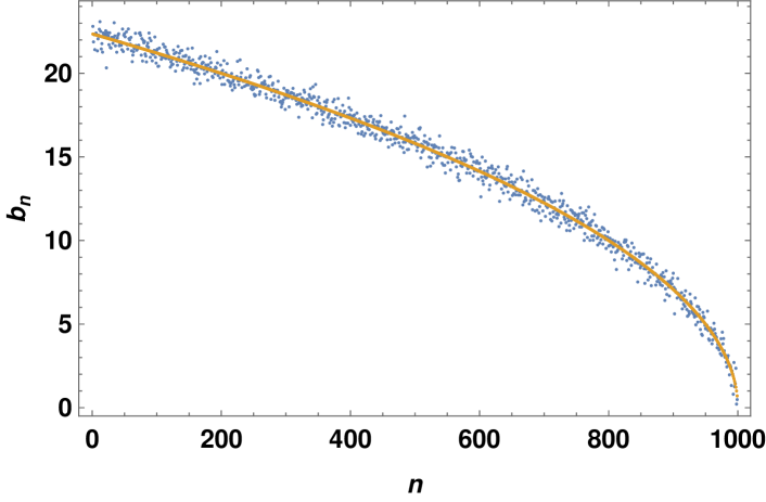
Figure 5: Variation of $b_{n}$ with $n$ for the case of FRM in the GOE. Here we have taken $\mathcal{N}=1000$. The solid line represents an approximate fitting for the $b_{n}$s, and is of the form $b_{n}=n_{1}(\mathcal{N}-n)^{n_{2}}$. We fix the unknown constants by using the exact SP in Eq. (7).

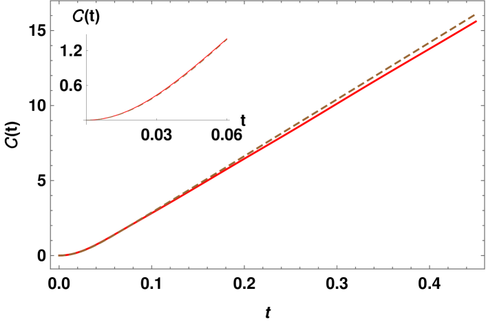
Figure 6: Early time evolution of SC when the quenched Hamiltonian is modeled with FRM in the GOE (the red curve). The dashed brown curve represents evolution when the two-level form factor is absent from the SP. In both cases, an early quadratic growth (shown clearly in the inset) merge into a linear growth at late times.

In Fig. 6 we have shown the early time behaviour of the SC for the FRM case and compared it with the evolution in the absence of the two-level form factor term. In both cases, the universal quadratic growth at very early times merged into linear growth at late times. The plots for SC with and without correlations between the energy levels match with each other for early times. This is due to the fact that in both cases, early time decay of the SP is governed by the Bessel function term (and hence a power law decay), and only after this initial power law decay, the effect of the two-level form factor manifests itself through the presence of the correlation hole in the SP, and thus the two curves for the SC differ from each other only after this time.

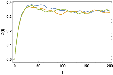
Figure 7: Evolution of the SC after a quench for three different RM in the GOE. Here $\mathcal{N}=1000$. The presence of the correlation hole in the SP is responsible for the peak in the SC.

Now to determine the unknown constants in the fitting curve for the $b_{n}$s we use the exact SP in Eq. (7), and compute the analytical expressions for the first few $b_{n}$s. Then we expand these expressions, taking $\mathcal{N}\gg 1$, and find out the dominant contribution of $\mathcal{N}$. For example, we have $b_{1}\approx\sqrt{\frac{\mathcal{N}}{2}}+\sqrt{\frac{1}{2\mathcal{N}}}+\mathcal{O}\big{(}\frac{1}{\mathcal{N}^{3/2}}\big{)}$. Comparing this with the fitting function in the limit $\mathcal{N}\gg 1$, we get $n_{1}=1/\sqrt{2}$ and $n_{2}=1/2$. This matching can be done by taking the analytical expressions for any higher order $b_{n}$s as well. Furthermore, we also notice that, when all the $b_{n}$s are expanded in powers of $\mathcal{N}$, the leading order contribution which survives in $\mathcal{N}\rightarrow\infty$ limit is proportional to $\sqrt{\mathcal{N}}$.

Time evolution of the SC at late times after quench with different FRM in the GOE is shown in Fig. 7. In all the cases, after an initial linear growth, the SC reaches a maximum value and then decays smoothly to a saturation value at late times. The peak in the SC for the FRM is due to the presence of the two-level form factor (and hence the correlation hole) in the SP. Furthermore, these features are consistent with the universal nature of the evolution of the SC of RM models discussed in Balasubramanian:2022tpr ; Erdmenger:2023shk .

IV Spread complexity in quenches of interacting spin-$1/2$ models

As we have discussed in the beginning of the previous subsection, the FRM is a somewhat unrealistic approximation of a realistic quantum system. However, the analytical expression for the SP for this FRM models, given in Eq. (7), can be used as a reference to obtain the expression for the SP under quench for more realistic 1-dimensional (1D) spin-$1/2$ quantum system, which shows chaotic behaviour in certain limits. Using numerical analysis, it is possible to obtain the SP of an initial state for sudden quench done on such 1D systems. Comparing these numerical results with the exact analytical expression for the SP for FRM it is possible to identify the following general dynamical features of quenched realistic many-body quantum systems Herrera6 ; Santos1 : (1) An initial power-law decay. (2) Presence of a correlation hole, where the SP decrease below the saturation value, and (3) Saturation at late times. The saturation value of the SP is equal to its infinite time average, i.e. $\bar{F}(t)\sim\sum_{n}\big{|}C_{0}^{n}\big{|}^{4}$, which, in turn, is just the inverse of the participation ratio of the initial state. In this section we demonstrate how these typical features of SP affect the evolution of SC at different times scales after when a sudden quench is performed in such a spin-$1/2$ system.

The Hamiltonian we consider is that of a one dimensional spin-$1/2$ system, which has two parts, $H=H_{0}+V$, i.e, the original Hamiltonian $H_{0}$, and a perturbation $V$, respectively. Here we assume these to be of the form Santos1

$$H_{0}=\sum_{j=1}^{L}h_{j}S_{j}^{z}~{},~{}~{}V=\sum_{j=1}^{L}\Big{(}S_{j}^{x}S_{j+1}^{x}+S_{j}^{y}S_{j+1}^{y}+S_{j}^{z}S_{j+1}^{z}\Big{)}~{},$$ (10)

where $L$ is the total number sites, and periodic boundary conditions are assumed to be applied. Since the parameter $h$ is non-zero, the system is disordered, and $h_{j}$ are random numbers taken from a uniform distribution $[-h,h]$. From the structure of the Hamiltonian, we see that before the quench, the coupling strength $g=0$, and after the quench it abruptly changes to $1$, so that the system is taken far from equilibrium through the quench.

Changing the disorder strength from an initial zero value, the Hamiltonian $H$ typically shows three distinct regions, a sharp transition from integrable (corresponding to zero disorder strength) to a chaotic domain, which is followed by a chaotic region. Finally, as the disorder strength is increased, the system acquires an intermediate region between chaotic and many-body localised phases Herrera8 . The level spacing distribution corresponding to the total Hamiltonian accordingly starts from Poisson, transforms to Wigner-Dyson, and then again goes back to Poisson as the disorder strength is increased.

In this paper we consider the largest subspace of the total Hilbert space of the system which has $\mathcal{S}_{z}=0$, and has dimension $N=L!/(L/2)!^{2}$, where $\mathcal{S}_{z}=\sum_{k}S^{z}_{k}$ is the total spin along the $z$ direction and is a conserved quantity for the Hamiltonian under consideration.

For the type of system under consideration, after a sudden quench, an analytical form for the SP can be obtained by comparing results from numerical simulations and the SP for the FRM given in Eq. (7), and this is given by Herrera9

$$\big{<}F(t)\big{>}_{h}=\frac{1-\big{<}\bar{F}\big{>}_{FRM}}{\mathcal{N}-1}\bigg{[}\mathcal{N}\frac{g(t)}{g(0)}-\mathcal{B}_{2}\Big{(}\frac{\sigma_{0}t}{\mathcal{N}}\Big{)}\bigg{]}+\big{<}\bar{F}\big{>}_{h}~{},$$ (11)

where the $\big{<}\cdots\big{>}_{h}$ now represents the disorder average, and the functional form for the function $g(t)$ is given by

$$g(t)=e^{-\sigma_{0}^{2}t^{2}}+\mathcal{A}\frac{1-e^{-\sigma_{0}^{2}t^{2}}}{\sigma_{0}^{2}t^{2}}~{}.$$ (12)

The constant $\mathcal{A}$ can be obtained by fitting this function with results for SP obtained from numerical simulations.

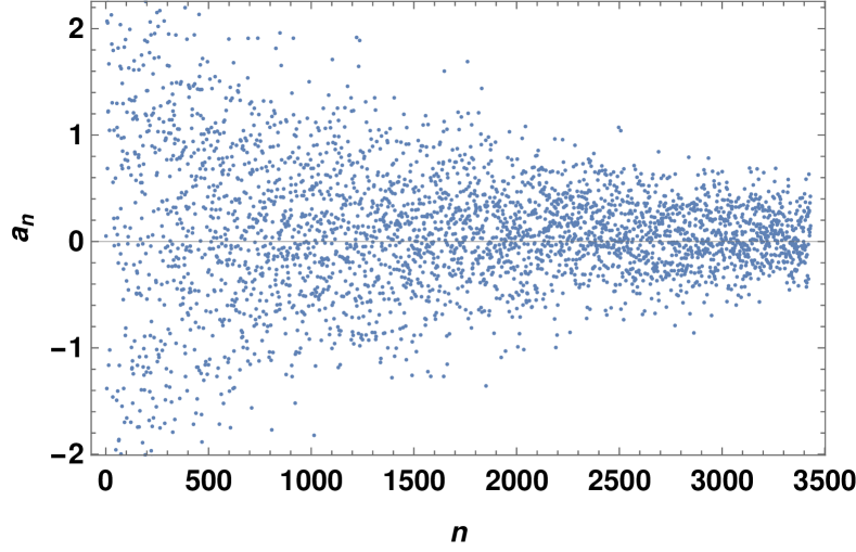
Figure 8: Variation of $a_{n}$ with $n$ for the quench in the integrable limit spin-$1/2$ model with disorder. Here we have taken $L=14$ and the initial state is a domain wall.

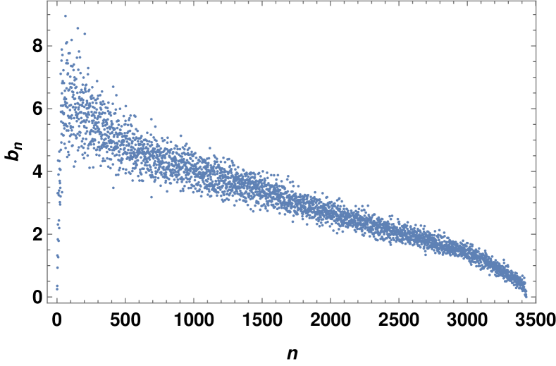
Figure 9: Variation of $b_{n}$ with $n$ for the quench in the integrable spin-$1/2$ model with disorder. Here we have taken $L=14$ and the initial state is a domain wall.

First we study the LCs and the SC of the spin-$1/2$ model in the non-chaotic case. As the initial state before the quench, we consider a domain wall, i.e., $\big{|}\uparrow\uparrow\uparrow\cdots\downarrow\downarrow\downarrow\big{>}$. The variation of the LCs $a_{n}$ and $b_{n}$ with respect to $n$, with $L=14$ sites are shown in Figs. 8 and 9, respectively. The $a_{n}$s are distributed almost uniformly around zero. On the other hand, the $b_{n}$s show initial sharp growth for lower values of $n$, reach a maximum peak, then decay gradually towards zero as we reach towards the end of the Krylov basis. As expected, after initial growth, the SC oscillates with time.

Next we consider quench in the non-integrable limit of this model. Here once again we take the domain wall as the initial state before the quench, and assume the disorder parameter to be $[-0.4,0.4]$. Here it is easy to see that, compared with the integrable limit of this model, the LCs are less randomly distributed. In particular, the variation of $b_{n}$ in this case is almost similar to the case of FRM shown in Fig. 5, though, there is an initial growth in the LCs for the spin-$1/2$ model which was not present in the FRM case. After the initial growth the $b_{n}$s reach a peak and then continue down to zero as we reach towards the end of the Krylov chain.

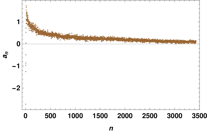
Figure 10: Variation of $a_{n}$ with $n$ for a quench in the chaotic limit of the spin-$1/2$ model with disorder. Here $L=14$ and the initial state is a domain wall.

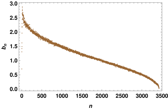
Figure 11: Variation of $b_{n}$ with $n$ for a quench in the chaotic spin-$1/2$ model with disorder. Here $L=14$ and the initial state is a domain wall.

The difference in the distribution of the LCs for the chaotic and non-chaotic domains can be better visualised from the histogram plots for these coefficients shown in Fig. 12 and 13 for $a_{n}$ and $b_{n}$ respectively. As can be clearly seen from these plots, when the disorder strength is away from the chaotic domain, the LCs are widely distributed compared to the case when the disorder strength is in the chaotic domain. The variance of the distribution of $a_{n}$ changes from $0.584$ in Fig. 8 to a subsequently lower value of $0.449$ corresponding to the chaotic domain in Fig. 10. Similarly, variance of the distribution of $b_{n}$ increases from $0.313$ in the chaotic case (Fig. 11) to $2.319$ (in Fig. 9) as the disorder strength is increased.

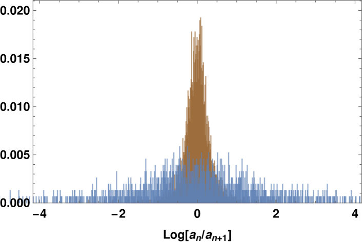
Figure 12: Histogram of the distribution of the LCs $a_{n}$ for the chaotic (brown) and non-chaotic domains (blue).

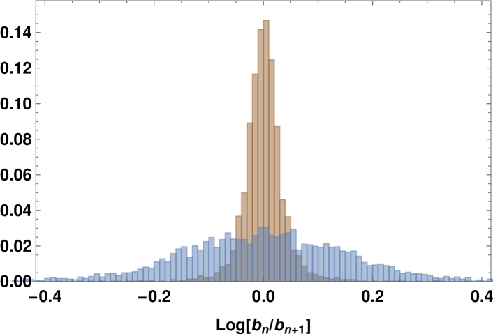
Figure 13: Histogram of the distribution of the LCs $b_{n}$ for the chaotic (brown) and non-chaotic (blue) domains.

The time evolution of the SC in this case is shown in Fig. 14 (for reference we have also shown the SC with $L=12$ as well). We notice that similar to the case of quench modeled with FRM, (shown in fig. 6) there is an initial linear growth at earlier times, however, the peak in the complexity is less pronounced compared to the FRM case. This behaviour of the SC can be understood from the fact that in the case of FRM, the correlation hole is deeper, while for the disordered spin-1/2 system, as the disorder strength is increased, the correlation hole becomes less pronounced, and fades for larger value of disorder. At late times, the SC fluctuates around the long time average value which depends on the dimension of the Krylov space, and hence on the system size. Therefore, as the strength of the disorder of the quenched spin chain is changed such that the system changes from integrable to chaotic, the SC can capture the necessary features of the corresponding phase in both the cases.

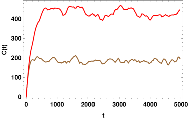
Figure 14: Time evolution of the SC after quench in a chaotic spin-$1/2$ model with disorder, for $L=12$ (brown) and $L=14$ (red). After a characteristics initial growth, the SC attains a saturation at late times. However, the peak in the complexity is almost absent in this case.

V Summary and Conclusions

In this paper, we have performed a detailed analysis of the evolution of the SC after quenches in interacting quantum many-body systems. We have shown that, for time scales that are small compared to the inverse of the width of the LDOS, the SC grows quadratically with time, irrespective of the final Hamiltonian or the initial state before the quench, with the rate of the growth being determined by the width of the LDOS (the width, in turn, is equal to the LC $b_{1}$). Behaviour of SC evolution in the next time scale is determined by the initial state, as well as the strength of the perturbation introduced via the quench. Exponential and Gaussian decays of the SP are two of the most commonly encountered behaviours of the SP after the initial quadratic decay. In the presence of strong perturbations, the SP shows Gaussian decay, and hence, the quadratic growth of the SC persists for a time longer than the inverse of the width of the LDOS. For sudden quenches in XX model and spin-$1/2$ systems with impurities, the quadratic growth can persists even up to the saturation point of the SP.

On the other hand, when the strength of the external perturbation is not strong, the initial quadratic decay merges into an exponential decay at late times. Using an interpolation formula connecting these two different decays, proposed in Flambaum , we have obtained the associated LC and the SC. The LC $b_{n}$s grows linearly with $n$ (whereas $a_{n}=0$), with the slope of the linear growth being determined by the width of the LDOS, and the initial quadratic growth of the SC merges into a linear growth at late times due to the presence of the exponential decay of the SP.

To understand the behaviour of SC at late times, we first modeled the quenched interacting system as a FRM in the GOE. The LC and the SC are then obtained by finding out the Hessenberg form of these RMs. Here, $a_{n}\approx 0$ and the $b_{n}$s can be fitted with a curve of the form $b_{n}=n_{1}(\mathcal{N}-n)^{n_{2}}$, where the two unknown constants have been determined by using the exact analytical expression in Eq. (7) available in the literature for the SP after a quench with FRM. Due to the presence of the correlation hole in the SP, the SC grows linearly with time, reaches a peak, after which it saturates to a lower constant value. These features of the SC evolution after quench are consistent with the behaviour for the same observed in Balasubramanian:2022tpr without such a quench.

As the next example, we considered quenches in an interacting spin-$1/2$ model in the presence of nearest neighbour interactions and disorder, which shows non-integrable behaviour in a particular range of the disorder parameter. For this model, we have obtained the full sets of LCs and the SC, in both the chaotic and the intermediate region between the chaotic and many-body localised phases, where the initial state before the quench is assumed to be a domain wall. Though the LCs show similar patterns in this case as with the FRM, the exact details are different. For example, away from the chaotic phase, the LCs are distributed randomly, whereas in the non-integrable phase, the distribution of the LCs are more compact. Importantly, the sequence of $b_{n}$s shows a linear growth for small values of $n$ and reaches a peak, a behaviour which is absent for the corresponding $b_{n}$ sequence for our FRM analysis. The analysis of the SC shows that in the chaotic phase of this model, it shows a linear growth at early times and saturation at late times, with the peak in the intermediate time between them being less pronounced in this case compared to that of the FRM.

Acknowledgements

The work of TS is supported in part by the USV Chair Professor position at the Indian Institute of Technology, Kanpur.

Appendix A Krylov basis construction and the spread complexity

In this appendix we briefly review the construction of the Krylov basis states using the Lanczos algorithm, and the subsequent definition of the SC of an arbitrary time evolved initial state after a quench under a new Hamiltonian. This procedure has been used in section III to find out the LC and the SC.

Assume that a sudden quench is performed on a quantum system at in initial time $t_{0}=0$, and subsequently, the state before the quench evolves under the new Hamiltonian $H$. In the Lanczos algorithm, one constructs new elements of the Krylov basis starting from an initial one by using the following procedure

$$\big{|}{K_{n+1}}\rangle=\frac{1}{b_{n+1}}\Big{[}\big{(}H-a_{n}\big{)}\big{|}{K_{n}}\rangle-b_{n}\big{|}{K_{n-1}}\rangle\Big{]}~{}.$$ (13)

Here, $\big{|}{K_{0}}\rangle=\big{|}{\psi_{0}}\rangle$, i.e., the first element of the Krylov basis is the initial state before the quench, and $H$ represents the Hamiltonian after the quench. The two sets of coefficients $a_{n}$ and $b_{n}$ are the LCs. The $b_{n}$s fix the normalization of the Krylov basis vectors at each step of the recursion and the $a_{n}$s are given by the expectation value of the post-quench Hamiltonian in the Krylov basis, i.e.,

$$a_{n}=\langle{K_{n}|H|K_{n}}\rangle~{}.$$ (14)

The recursion stops when $b_{n}=0$ for some value of $n$.

Now we can expand the time evolved state after quench in terms of the Krylov basis

$$\big{|}{\psi(t)}\rangle=\sum_{n}\phi_{n}(t)\big{|}{K_{n}}\rangle~{},$$ (15)

where, using the Schrodinger equation satisfied by the Hamiltonian $H$, one can show that the expansion coefficients $\phi_{n}(t)$ satisfy the following discrete Schrodinger equation

$$i\dot{\phi}_{n}(t)=a_{n}\phi_{n}(t)+b_{n}\phi_{n-1}(t)+b_{n+1}\phi_{n+1}(t)~{}.$$ (16)

Here, an overdot represents a derivative with respect to time. In Balasubramanian:2022tpr it was proved that if we consider cost functions of the form $\mathcal{C}_{B}(t)=\sum_{n}n|\langle{\psi(t)|B_{n}}\rangle|^{2}$, to indicate the spread of a time evolved wavefunction in terms of a complete orthonormal basis $\big{|}B_{n}\rangle$, then this cost is minimised when evaluated in the Krylov basis $\big{|}K_{n}\rangle$. Therefore, we arrive at the definition of the SC as the minimum of the above cost as

$$\mathcal{C}(t)=\sum_{n}n|\langle{\psi(t)|K_{n}}\rangle|^{2}=\sum_{n}n|\phi_{n}(t)|^{2}~{}.$$ (17)

We conclude this appendix by briefly outlining the procedure of obtaining the LCs from the moments of the return amplitude $\mathcal{S}(t)$ following Viswanath . Consider the expansion of the auto-correlation function in terms of the moments

$$\mathcal{S}(t)=\sum_{n}^{\infty}M_{n}^{*}\frac{t^{n}}{n!}~{}.$$ (18)

The next step is to construct two sets of auxiliary matrices $L_{k}^{(n)}$ and $M_{k}^{(n)}$ from the moments $M_{n}^{*}$. The two sets of LCs are then obtained from these auxiliary matrices as $b_{n}=\sqrt{M_{n}^{(n)}}$ and $a_{n}=-L_{n}^{(n)}$, where we have to chose initial conditions properly so that $b_{0}=0$ Balasubramanian:2022tpr ; Viswanath . Knowing the full set of LCs we can then solve the discrete Schrodinger equation in (16) to obtain the time-dependent expansion coefficients $\phi_{n}(t)$, and subsequently obtain the complexity by evaluating the sum in Eq. (17).

References

- (1) M. A. Nielsen, arXiv:quant-ph/0502070 [quant-ph].
- (2) M. A. Nielsen, M. R. Dowling, M. Gu, and A. M. Doherty, Science 311 (2006) 1133.
- (3) M. A. Nielsen and M. R. Dowling, arXiv:quant-ph/0701004.
- (4) R. Jefferson and R. C. Myers. JHEP 10 (2017), 107
- (5) R. Khan, C. Krishnan and S. Sharma, Phys. Rev. D 98 (2018) no.12, 126001.
- (6) L. Hackl and R. C. Myers, JHEP 07 (2018), 139.
- (7) A. Bhattacharyya, A. Shekar and A. Sinha, JHEP 10 (2018), 140.
- (8) S. Chapman and G. Policastro, Eur. Phys. J. C 82 (2022) no.2, 128.
- (9) D. E. Parker, X. Cao, A. Avdoshkin, T. Scaffidi and E. Altman, Phys. Rev. X 9 (2019) no.4, 041017.
- (10) J. L. F. Barbón, E. Rabinovici, R. Shir and R. Sinha, JHEP 10 (2019), 264.
- (11) B. Bhattacharjee, X. Cao, P. Nandy and T. Pathak, JHEP 05 (2022), 174.
- (12) A. Dymarsky and A. Gorsky, Phys. Rev. B 102 (2020) no.8, 085137.
- (13) A. Dymarsky and M. Smolkin, Phys. Rev. D 104 (2021) no.8, L081702.
- (14) A. Kundu, V. Malvimat and R. Sinha, [arXiv:2303.03426 [hep-th]].
- (15) A. Bhattacharya, P. Nandy, P. P. Nath and H. Sahu, JHEP 12 (2022), 081.
- (16) B. Bhattacharjee, X. Cao, P. Nandy and T. Pathak, JHEP 03 (2023), 054.
- (17) A. Bhattacharya, P. Nandy, P. P. Nath and H. Sahu, [arXiv:2303.04175 [quant-ph]].
- (18) A. Bhattacharyya, D. Ghosh and P. Nandi, [arXiv:2306.05542 [hep-th]].
- (19) J. Kim, J. Murugan, J. Olle and D. Rosa, Phys. Rev. A 105 (2022) no.1, L010201.
- (20) K. Hashimoto, K. Murata, N. Tanahashi and R. Watanabe, [arXiv:2305.16669 [hep-th]].
- (21) H. A. Camargo, V. Jahnke, H. S. Jeong, K. Y. Kim and M. Nishida, [arXiv:2306.11632 [hep-th]].
- (22) H. A. Camargo, V. Jahnke, K. Y. Kim and M. Nishida, [arXiv:2212.14702 [hep-th]].
- (23) A. Avdoshkin, A. Dymarsky and M. Smolkin, [arXiv:2212.14429 [hep-th]].
- (24) D. J. Yates and A. Mitra, Phys. Rev. B 104 (2021) no.19, 195121.
- (25) P. Caputa and S. Datta, JHEP 12 (2021), 188 [erratum: JHEP 09 (2022), 113].
- (26) D. Patramanis, PTEP 2022 (2022) no.6, 063A01.
- (27) F. B. Trigueros and C. J. Lin, SciPost Phys. 13 (2022) no.2, 037.
- (28) E. Rabinovici, A. Sánchez-Garrido, R. Shir and J. Sonner, JHEP 03 (2022), 211.
- (29) M. Alishahiha and S. Banerjee, [arXiv:2212.10583 [hep-th]].
- (30) K. Adhikari, S. Choudhury and A. Roy, [arXiv:2204.02250 [hep-th]].
- (31) K. Adhikari and S. Choudhury, Fortsch. Phys. 70 (2022) no.12, 2200126.
- (32) W. Mück and Y. Yang, Nucl. Phys. B 984 (2022), 115948.
- (33) E. Rabinovici, A. Sánchez-Garrido, R. Shir and J. Sonner, JHEP 07 (2022), 151.
- (34) B. Bhattacharjee, S. Sur and P. Nandy, Phys. Rev. B 106 (2022) no.20, 205150.
- (35) A. Chattopadhyay, A. Mitra and H. J. R. van Zyl, [arXiv:2302.10489 [hep-th]].
- (36) B. Bhattacharjee, [arXiv:2302.07228 [quant-ph]].
- (37) B. Bhattacharjee, P. Nandy and T. Pathak, [arXiv:2210.02474 [hep-th]].
- (38) K. Takahashi and A. del Campo, [arXiv:2302.05460 [quant-ph]].
- (39) D. Patramanis and W. Sybesma, [arXiv:2306.03133 [quant-ph]].
- (40) M. J. Vasli, K. Babaei Velni, M. R. Mohammadi Mozaffar, A. Mollabashi and M. Alishahiha, [arXiv:2307.08307 [hep-th]].
- (41) A. Bhattacharyya, S. S. Haque, G. Jafari, J. Murugan and D. Rapotu, [arXiv:2307.15495 [hep-th]].
- (42) A. A. Nizami and A. W. Shrestha, [arXiv:2305.00256 [quant-ph]].
- (43) Z. Y. Fan, [arXiv:2306.16118 [hep-th]].
- (44) V. Balasubramanian, P. Caputa, J. M. Magan and Q. Wu, Phys. Rev. D 106 (2022) no.4, 046007.
- (45) J. Erdmenger, S. K. Jian and Z. Y. Xian, [arXiv:2303.12151 [hep-th]].
- (46) P. Caputa and S. Liu, Phys. Rev. B 106, 195125 (2022).
- (47) P. Caputa, N. Gupta, S. S. Haque, S. Liu, J. Murugan and H. J. R. Van Zyl, JHEP 01 (2023), 120.
- (48) M. Afrasiar, J. K. Basak, B. Dey, K. Pal, and K. Pal, arXiv:2208.10520 [hep-th].
- (49) M. Gautam, N. Jaiswal and A. Gill, [arXiv:2305.12115 [quant-ph]].
- (50) K. Pal, K. Pal, A. Gill and T. Sarkar, [arXiv:2304.09636 [quant-ph]].
- (51) S. Nandy, B. Mukherjee, A. Bhattacharyya and A. Banerjee, [arXiv:2305.13322 [quant-ph]].
- (52) D. W. F. Alves and G. Camilo, JHEP 06, 029 (2018).
- (53) H. A. Camargo, P. Caputa, D. Das, M. P. Heller, and R. Jefferson, Phys. Rev. Lett. 122, 081601 (2019).
- (54) G. Di Giulio and E. Tonni, JHEP 05 (2021), 022.
- (55) N. Jaiswal, M. Gautam and T. Sarkar, J. Stat. Mech. 2207 (2022) no.7, 073105.
- (56) K. Pal, K. Pal and T. Sarkar, Phys. Rev. E 107 (2023) no.4, 044130.
- (57) M. Gautam, N. Jaiswal, A. Gill and T. Sarkar, [arXiv:2207.14090 [quant-ph]].
- (58) T. Ali, A. Bhattacharyya, S. Shajidul Haque, E. H. Kim and N. Moynihan, Phys. Lett. B 811 (2020), 135919.
- (59) T. Ali, A. Bhattacharyya, S. Shajidul Haque, E. H. Kim and N. Moynihan, JHEP 04 (2019), 087.
- (60) K. Pal, K. Pal, A. Gill and T. Sarkar, [arXiv:2206.03366 [quant-ph]].
- (61) V. S. Viswanath, G. Muller, The Recursion Method Application to Many-Body Dynamics, Springer (1994).
- (62) C. Lanczos, J. Res. Natl. Bur. Stand. B 45 (1950), 255-282.
- (63) A. Peres, Phys. Rev. A 30 1610 (1984).
- (64) N. R. Cerruti and S. Tomsovic, Phys. Rev. Lett. 88 054103 (2002).
- (65) E. J. Torres-Herrera and L. F. Santos, Phys. Rev. A 89 043620 (2014).
- (66) J. Emerson, Y. S. Weinstein, S. Lloyd and D. G. Cory Phys. Rev. Lett. 89 284102 (2002).
- (67) E. J. Torres-Herrera, M. Vyas and L. F. Santos, New J. Phys. 16 063010 (2014).
- (68) E. J. Torres-Herrera and L. F. Santos, Phys. Rev. E 89 (2014), 062110.
- (69) M. Tavora, E. J. Torres-Herrera and L. F. Santos, Phys. Rev. A 94 041603 (2016).
- (70) M. Tavora, E. J. Torres-Herrera and L. F. Santos, Phys. Rev. A 95 013604 (2017).
- (71) L. F. Santos, E. J. Torres-Herrera, AIP Conference Proceedings 1912, 020015 (2017).
- (72) V. V. Flambaum and F. M. Izrailev, Phys. Rev. E 64, 026124 (2001).
- (73) F. M. Izrailev and A. Castaneda-Mendoza, Phys. Lett. A 350, 355 (2006).
- (74) V.V. Flambaum, Aust. J. Phys. 53, N4 (2000).
- (75) P. Caputa, J.M. Magan and D. Patramanis, Phys. Rev. Res. 4 (2022) 013041.
- (76) M. L. Mehta, Random Matrices (Academic Press, Boston, 1991).
- (77) T. Guhr, A. Mueller-Groeling and H. A. Weidenmuller, Phys. Rep. 299 (1998), p. 189.
- (78) A. Kar, L. Lamprou, M. Rozali and J. Sully, JHEP 01 (2022), 016.
- (79) E. J. Torres-Herrera, J. Karp, M Tavora, and L. F. Santos, Entropy 2016, 18 (10), 359.
- (80) E. J. Torres-Herrera and L. F. Santos, Phil. Trans. R.Soc. A 375: 20160434.
- (81) L. Leviandier, M. Lombardi, R. Jost and J. P. Pique, Phys. Rev. Lett. 56 (1986), pp. 2449–2452.
- (82) T. Guhr and H. Weidenmuller, Chem. Phys. 146 (1990), pp. 21 – 38.
- (83) Y. Alhassid and R. D. Levine, Phys. Rev. A 46 (1992), pp. 4650–4653.
- (84) Torres-Herrera EJ, Santos LF. 2014, Phys. Rev. A 90, 033623 (2014).
- (85) E. J. Torres-Herrera, A. M. Garcia-Garcia and L. F. Santos, New J. Phys. 16 063010 (2014).
- (86) E. J. Torres-Herrera and L. F. Santos, Ann. Phys. (Berlin) 529, 1600284 (2017).
- (87) E. J. Torres-Herrera, A. M. Garcia-Garcia and L. F. Santos, Phys. Rev. B 97, 060303(R) (2018).