Sierpiński fractals and the dimension of their Laplacian spectrum

Abstract

We estabish rigorous estimates for the Hausdorff dimension of the spectra of Laplacians associated to Sierpiński lattices and infinite Sierpiński gaskets and other post-critically finite self-similar sets.

Dedicated to Károly Simon on the occasion of his 60+1st birthday

1 Introduction

The study of the Laplacian on manifolds has been a very successful area of mathematical analysis for over a century, combining ideas from topology, geometry, probability theory and harmonic analysis. A comparatively new development is the theory of a Laplacian for certain types of naturally occurring fractals, see [29, 26, 31, 9, 28, 12, 21], to name but a few. A particularly well-known example is the following famous set.

Definition 1.1.

The Sierpiński triangle $\mathcal{T}\subset\mathbb{R}^{2}$ (see Figure 1(a)) is the smallest non-empty compact set such that $\bigcup_{i=1}^{3}T_{i}(\mathcal{T})=\mathcal{T}$ where $T_{1},T_{2},T_{3}\colon\mathbb{R}^{2}\to\mathbb{R}^{2}$ are the affine maps

$$T_{1}(x,y) =\left(\frac{x}{2},\frac{y}{2}\right)\qquad T_{2}(x,y)=\left(\frac{x}{2}+\frac{1}{2},\frac{y}{2}\right)$$

$$T_{3}(x,y) =\left(\frac{x}{2}+\frac{1}{4},\frac{y}{2}+\frac{\sqrt{3}}{4}\right).$$

           

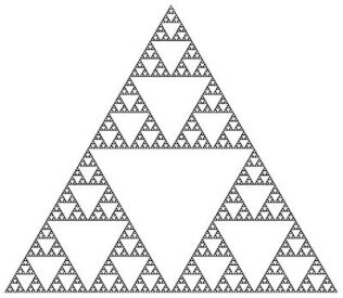
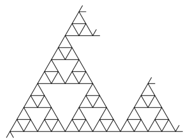
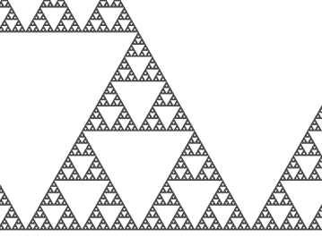
Figure 1: (a) The standard Sierpiński triangle $\mathcal{T}$; (b) The Sierpiński lattice ${\mathcal{L}}$; and (c) The infinite Sierpiński triangle $\mathcal{T}^{\infty}$.

A second object which will play a role is the following infinite graph.

Definition 1.2.

Let $V_{0}=\{(0,0),(1,0),(\frac{1}{2},\frac{\sqrt{3}}{2})\}$ be the vertices of $\mathcal{T}$ and define $V_{n}=\bigcup_{i=1}^{3}T_{i}(V_{n-1})$. Further, fix a sequence $\omega=(\omega_{n})_{n\in\mathbb{N}}\subset\{1,2,3\}^{\mathbb{N}}$, and let

$$V^{\infty}=\bigcup_{i=1}^{\infty}V^{n}\text{ with }V^{n}=T_{\omega_{1}}^{-1}\circ\cdots\circ T_{\omega_{n}}^{-1}(V_{n}),$$

where we use the inverses

$$T_{1}^{-1}(x,y) =\left(2x,2y\right)\qquad T_{2}^{-1}(x,y)=\left(2x-1,2y\right)$$

$$T_{3}^{-1}(x,y) =\left(2x-\frac{1}{2},2y-\frac{\sqrt{3}}{2}\right).$$

The definition of $V^{\infty}$ depends on the choice of $\omega$, however as will be explained below, the relevant results do not, allowing us to omit the dependence in our notation. The points in $V^{\infty}$ correspond to the vertices of an infinite graph $\mathcal{L}$ called a Sierpiński lattice for which the edges correspond to pairs of vertices $(v,v^{\prime})$, with $v,v^{\prime}\in V^{\infty}$ such that $\|v-v^{\prime}\|_{2}=1$ (see Figure 1(b)). Equivalently, $\mathcal{L}$ has an edge $(v,v^{\prime})$ if and only if

$$v,v^{\prime}\in T_{\omega_{1}}^{-1}\circ\cdots\circ T_{\omega_{n}}^{-1}\circ T_{i_{n}}\circ\cdots\circ T_{i_{1}}(V_{0})$$

for some $i_{1},\ldots,i_{n}\in\{1,2,3\}$, $n\geqslant 0$.

Finally, we will also be interested in infinite Sierpiński gaskets, which can be defined similarly to Sierpiński lattices as follows.

Definition 1.3.

For a fixed sequence $\omega=(\omega_{n})_{n\in\mathbb{N}}$, we define an infinite Sierpiński gasket to be the unbounded set $\mathcal{T}^{\infty}$ given by

$$\mathcal{T}^{\infty}=\bigcup_{n=0}^{\infty}\mathcal{T}^{n},\text{ with }\mathcal{T}^{n}=T_{\omega_{1}}^{-1}\circ\cdots\circ T_{\omega_{n}}^{-1}(\mathcal{T}),$$

which is a countable union of copies of the standard Sierpiński triangle $\mathcal{T}$ (see Figure 1(c)). As for Sierpiński lattices, the definition of $\mathcal{T}^{\infty}$ depends on the choice of $\omega$, but we omit this dependence in our notation as the cited results hold independently of it.

The maps $T_{1}$, $T_{2}$ and $T_{3}$ are similarities on $\mathbb{R}^{2}$ with respect to the Euclidean norm, and more precisely

$$\|T_{i}(x_{1},y_{1})-T_{i}(x_{2},y_{2})\|_{2}=\frac{1}{2}\|(x_{1},y_{1})-(x_{2},y_{2})\|_{2}$$

for $(x_{1},y_{1}),(x_{2},y_{2})\in\mathbb{R}^{2}$ and $i=1,2,3$, and thus by Moran’s theorem the Hausdorff dimension of $\mathcal{T}$ has the explicit value $\dim_{H}(\mathcal{T})=\frac{\log 3}{\log 2}$ [8]. We can easily give the Hausdorff dimensions of the other spaces. It is clear that $\dim_{H}(\mathcal{L})=1$ and since an infinite Sierpiński gasket $\mathcal{T}^{\infty}$ consists of countably many copies of $\mathcal{T}$ it follows that we also have $\dim_{H}(\mathcal{T}^{\infty})=\frac{\log 3}{\log 2}$.

In this note we are concerned with other fractal sets closely associated to the infinite Sierpiński gasket $\mathcal{T}^{\infty}$ and the Sierpiński lattice $\mathcal{L}$, for which the Hausdorff dimensions are significantly more difficult to compute.

In §2 we will describe how to associate to $\mathcal{T}$ a Laplacian $\Delta_{\mathcal{T}}$ which is a linear operator defined on suitable functions $f\colon\mathcal{T}\to\mathbb{R}$. An eigenvalue $\lambda\geqslant 0$ for $-\Delta_{\mathcal{T}}$ on the Sierpiński triangle is then a solution to the basic identity

$$\Delta_{\mathcal{T}}f+\lambda f=0.$$

The spectrum $\sigma(-\Delta_{\mathcal{T}})\subset\mathbb{R}^{+}$ of $-\Delta_{\mathcal{T}}$ is a countable set of eigenvalues. In particular, its Hausdorff dimension satisfies $\dim_{H}(\sigma(-\Delta_{\mathcal{T}}))=0$. A nice account of this theory appears in the survey note of Strichartz [29] and his book [30].

By contrast, in the case of the infinite Sierpiński gasket and the Sierpiński lattice there are associated Laplacians, denoted $\Delta_{\mathcal{T}^{\infty}}$ and $\Delta_{\mathcal{L}}$, respectively, with spectra $\sigma(-\Delta_{\mathcal{T}^{\infty}})\subset\mathbb{R}^{+}$ and $\sigma(-\Delta_{\mathcal{L}})\subset\mathbb{R}^{+}$ which are significantly more complicated. In particular, their Hausdorff dimensions are non-zero and therefore their numerical values are of potential interest. However, unlike the case of the dimensions of the original sets $\mathcal{T}^{\infty}$ and $\mathcal{L}$, there is no clear explicit form for this quantity. Fortunately, using thermodynamic methods we can estimate the Hausdorff dimension numerically to very high precision.

Theorem 1.4.

The Hausdorff dimension of $\sigma(-\Delta_{\mathcal{T}^{\infty}})$ and $\sigma(-\Delta_{\mathcal{L}})$ satisfy

$$\dim_{H}(\sigma(-\Delta_{\mathcal{T}^{\infty}}))=\dim_{H}\left(\sigma(-\Delta_{\mathcal{L}})\right)=0.55161856837246\ldots$$

A key point in our approach is that we have rigorous bounds, and the value in the above theorem is accurate to the number of decimal places presented. We can actually estimate this Hausdorff dimension to far more decimal places. To illustrate this, in the final section we give an approximation to $100$ decimal places.

It may not be immediately obvious what practical information the numerical value of the Hausdorff dimension gives about the sets $\mathcal{T}^{\infty}$ and $\mathcal{L}$ but it may have the potential to give an interesting numerical characteristic of the spectra. Beyond pure fractal geometry, the spectra of Laplacians on fractals are also of practical interest, for instance in the study of vibrations in heterogeneous and random media, or the design of so-called fractal antennas [6, 10].

We briefly summarize the contents of this note. In §2 we describe some of the background for the Laplacian on the Sierpiński graph. In particular, in §2.3 we recall the basic approach of decimation which allows $\sigma(\Delta_{\mathcal{T}})$ to be expressed in terms of a polynomial $R_{\mathcal{T}}(x)$. Although we are not directly interested in the zero-dimensional set $\sigma(-\Delta_{\mathcal{T}})$, the spectra of $\sigma(-\Delta_{\mathcal{T}^{\infty}})$ and $\sigma(-\Delta_{\mathcal{L}})$ actually contain a Cantor set $\mathcal{J}_{\mathcal{T}}\subset[0,5]$, the so-called Julia set associated to the polynomial $R_{\mathcal{T}}(x)$.

As one would expect, other related constructions of fractal sets have similar spectral properties and their dimension can be similarly studied. In §3 we consider higher-dimensional Sierpiński simplices, post-critically finite fractals, and an analogous problem where we consider the spectrum of the Laplacian on infinite graphs (e.g., the Sierpiński graph and the Pascal graph). In §4 we recall the algorithm we used to estimate the dimension and describe its application. This serves to both justify our estimates and also to use them as a way to illustrate a method with wider applications.

2 Spectra of the Laplacians

2.1 Energy forms

There are various approaches to defining the Laplacian $\Delta_{\mathcal{T}}$ on $\mathcal{T}$. We will use one of the simplest ones, using energy forms.

Following Kigami [12] the definition of the spectrum of the Laplacian for the Sierpiński gasket $\mathcal{T}$ involves a natural sequence of finite graphs $X_{n}$ with

$$X_{0}\subset X_{1}\subset X_{2}\subset\cdots\subset\bigcup_{n}X_{n}\subset\overline{\bigcup_{n}X_{n}}=:\mathcal{T},$$

the first three of which are illustrated in Figure 2. To this end, let

$$V_{0}=\left\{(0,0),(1,0),\left(\frac{1}{2},\frac{\sqrt{3}}{2}\right)\right\}$$

be the three vertices of $X_{0}$. The vertices of $X_{n}$ can be defined iteratively to be the set of points satisfying

$$V_{n}=T_{1}(V_{n-1})\cup T_{2}(V_{n-1})\cup T_{3}(V_{n-1})\quad\hbox{ for }n\geqslant 1.$$

Figure 2: The first three graphs for the Sierpiński triangle.

We denote by $\ell^{2}(V_{n})$ (for $n\geqslant 0$) the real valued functions $f\colon V_{n}\to\mathbb{R}$ (where the $\ell^{2}$ notation is used for consistency with the infinite-dimensional case despite having no special significance for finite sets).

Definition 2.1.

To each of the finite graphs $X_{n}$ ($n\geqslant 0$) we can associate bilinear forms $\mathcal{E}_{n}\colon\ell^{2}(V_{n})\times\ell^{2}(V_{n})\to\mathbb{R}$ called self-similar energy forms given by

$$\mathcal{E}_{n}(f,g)=c_{n}\sum_{x\sim_{n}y}(f(x)-f(y))(g(x)-g(y)),$$ (2.1)

where $x,y\in V_{n}$ are vertices of $X_{n}$, and $x\sim_{n}y$ denotes neighbouring edges in $X_{n}$. In particular, $x\sim_{n}y$ precisely when there exists $x^{\prime},y^{\prime}\in V_{n-1}$ and $i\in\{1,2,3\}$ such that $x=T_{i}(x^{\prime})$ and $y=T_{i}(y^{\prime})$. The value $c_{n}>0$ denotes a suitable scaling constant. With a slight abuse of notation, we also write $\mathcal{E}_{n}(f):=\mathcal{E}_{n}(f,f)$ for the corresponding quadratic form $\ell^{2}(V_{n})\to\mathbb{R}$.

To choose the values $c_{n}>0$ (for $n\geqslant 0$) we want the sequence of bilinear forms $(\mathcal{E}_{n})_{n=0}^{\infty}$ to be consistent by asking that for any $f_{n-1}\colon V_{n-1}\to\mathbb{R}$ (for $n\geqslant 1$) we have

$$\mathcal{E}_{n-1}(f_{n-1})=\mathcal{E}_{n}(f_{n}),$$

where $f_{n}\colon V_{n}\to\mathbb{R}$ denotes an extension which satisfies:

1. $f_{n}(x)=f_{n-1}(x)$ for $x\in V_{n-1}$; and

2. $f_{n}$ satisfying (a) minimizes $\mathcal{E}_{n}(f_{n})$ (i.e., $\mathcal{E}_{n}(f_{n})=\min_{f\in\ell^{2}(V_{n})}\mathcal{E}_{n}(f)$).

The following is shown in [30], for example.

Lemma 2.2.

The family $(\mathcal{E}_{n})_{n=0}^{\infty}$ is consistent if we choose $c_{n}=\left(\frac{5}{3}\right)^{n}$ in (2.1).

The proof of this lemma is based on solving families of simultaneous equations arising from (a) and (b). We can now define a bilinear form for functions on $\mathcal{T}$ using the consistent family of bilinear forms $(\mathcal{E}_{n})_{n=0}^{\infty}$.

Definition 2.3.

For any continuous function $f\colon\mathcal{T}\to\mathbb{R}$ we can associate the limit

$$\mathcal{E}(f):=\lim_{n\to+\infty}\mathcal{E}_{n}(f)\in[0,+\infty]$$

and let $\hbox{\rm dom}(\mathcal{E})=\{f\in C(\mathcal{T}):\mathcal{E}(f)<+\infty\}$.

Remark 2.4.

We can consider eigenfunctions $f\in\hbox{\rm dom}(\mathcal{E})$ which satisfy Dirichlet boundary conditions (i.e., $f|V_{0}=0$).

2.2 Laplacian for $\mathcal{T}$

To define the Laplacian $\Delta_{\mathcal{T}}$ the last ingredient is to consider an inner product defined using the natural measure $\mu$ on the Sierpiński triangle $\mathcal{T}$.

Definition 2.5.

Let $\mu$ be the natural measure on $\mathcal{T}$ such that

$$\mu\left(T_{i_{1}}\circ\cdots\circ T_{i_{n}}\hbox{\rm co}(V_{0})\right)=\frac{1}{3^{n}}\quad\hbox{ for }i_{1},\dots,i_{n}\in\{1,2,3\},$$

where $\hbox{\rm co}(V_{0})$ is the convex hull of $V_{0}$, i.e., the filled-in triangle.

In particular, $\mu$ is the Hausdorff measure for $\mathcal{T}$, and the unique measure on $\mathcal{T}$ for which

$$T_{i}^{*}\mu=\frac{1}{3}\mu\quad\hbox{ for }i=1,2,3.$$

The subspace $\hbox{\rm dom}(\mathcal{E})\subset L^{2}(\mathcal{T},\mu)$ is a Hilbert space. Using the measure $\mu$ and the bilinear form $\mathcal{E}$ we recall the definition of the Laplacian $\Delta_{\mathcal{T}}$.

Definition 2.6.

For $u\in\hbox{\rm dom}(\mathcal{E})$ which vanishes on $V_{0}$ we can define the Laplacian to be a continuous function $\Delta_{\mathcal{T}}u\colon\mathcal{T}\to\mathbb{R}$ such that

$$\mathcal{E}(u,v)=-\int(\Delta_{\mathcal{T}}u)vd\mu$$

for any $v\in\hbox{\rm dom}(\mathcal{E})$.

Remark 2.7.

For each finite graph $X_{n}$, the spectrum $\sigma(-\Delta_{X_{n}})$ for the graph Laplacian $\Delta_{X_{n}}$ will consist of a finite number of solutions of the eigenvalue equation

$$\Delta_{X_{n}}f+\lambda f=0.$$ (2.2)

This is easy to see because $V_{n}$ is finite and thus the space $\ell^{2}(V_{n})$ is finite-dimensional and so the graph Laplacian can be represented as a matrix. There is then an alternative pointwise formulation of the Laplacian of the form

$$\Delta_{\mathcal{T}}u(x)=\frac{3}{2}\lim_{n\to+\infty}5^{n}\Delta_{X_{n}}u(x)$$ (2.3)

where $x\in\bigcup_{n=1}^{\infty}V_{n}\setminus V_{0}$. The eigenvalue equation $\Delta_{\mathcal{T}}u+\lambda u=0$ then has admissible solutions provided $u,\Delta_{\mathcal{T}}u\in C(\mathcal{T})$. A result of Kigami is that $u\in\hbox{\rm dom}(\mathcal{E})$ if and only if the convergence in (2.3) is uniform [13].

2.3 Spectral decimation for $\sigma(-\Delta_{\mathcal{T}})$

We begin by briefly recalling the fundamental notion of spectral decimation introduced by [21, 22, 2], which describes the spectrum $\sigma(-\Delta_{\mathcal{T}})$.

         

Figure 3: The polynomial $R_{\mathcal{T}}(x)$ and the contracting inverse branches $S_{-1,\mathcal{T}}$ and $S_{+1,\mathcal{T}}$ for the Sierpiński triangle $\mathcal{T}$.

Definition 2.8.

Given the polynomial $R_{\mathcal{T}}\colon[0,5]\to\mathbb{R}$ defined by

$$R_{\mathcal{T}}(x)=x(5-x),$$

we can associate local inverses (see Figure 3) $S_{-1,\mathcal{T}},S_{+1,\mathcal{T}}\colon[0,5]\to[0,5]$ of the form

$$S_{\epsilon,\mathcal{T}}(x)=\frac{5}{2}+\frac{\epsilon}{2}\sqrt{25-4x}\quad\hbox{ for }\epsilon=\pm 1.$$ (2.4)

The process of spectral decimation (see [30, §3.2] or [9]) describes the eigenvalues of $-\Delta_{\mathcal{T}}$ as renormalized limits of (certain) eigenvalue sequences of $-\Delta_{X_{n}},n\in\mathbb{N}$. These eigenvalues, essentially, follow the recursive equality $\lambda_{n+1}=S_{\pm 1,\mathcal{T}}(\lambda_{n})$, while the corresponding eigenfunctions of $-\Delta_{X_{n+1}}$ are such that their restrictions to $V_{n}$ are eigenfunctions for $-\Delta_{X_{n}}$. Thus, the eigenvalue problem can be solved inductively, constructing solutions $f$ to the eigenvalue equation (2.2) at level $n+1$ from solutions at level $n\in\mathbb{N}$. The values of $f$ at vertices in $V_{n+1}\setminus V_{n}$ are obtained from solving the additional linear equations that arise from the eigenvalue equation $\Delta_{X_{n+1}}f+\lambda f=0$, which allows for exactly two solutions. The exact limiting process giving rise to eigenvalues of $-\Delta_{\mathcal{T}}$ is described by the following result.

Proposition 2.9 ([9, 21, 4]).

Every solution $\lambda\in\mathbb{R}$ to the eigenvalue equation

$$\Delta_{\mathcal{T}}u+\lambda u=0$$ (2.5)

can be written as

$$\lambda=\frac{3}{2}\lim_{m\to+\infty}5^{m+c}\lambda_{m},$$ (2.6)

for a sequence $(\lambda_{m})_{m\geqslant m_{0}}$ and a positive integer $c\in\mathbb{N}_{0}$ satisfying

1. $\lambda_{m_{0}}=2$ and $c=0$, or $\lambda_{m_{0}}=5$ and $c\geqslant 1$, or $\lambda_{m_{0}}=3$ and $c\geqslant 2$;

2. $\lambda_{m}=\lambda_{m+1}(5-\lambda_{m+1})=R_{\mathcal{T}}(\lambda_{m+1})$ for all $m\geqslant m_{0}$; and

3. the limit (2.6) is finite.

Conversely, the limit of every such sequence gives rise to a solution of (2.5).

We remark that equivalently, the sequence $(\lambda_{m})_{m\geqslant m_{0}}$ could be described recursively as $\lambda_{m+1}=S_{\epsilon_{m},\mathcal{T}}(\lambda_{m})$ where $\epsilon_{m}\in\{\pm 1\}$ for $m\geqslant m_{0}$. The finiteness of the limit (2.6) is equivalent to there being an $m^{\prime}\geqslant m_{0}$ such that $\epsilon_{m}=-1$ for all $m\geqslant m^{\prime}$.

2.4 Spectrum of the Laplacian for Sierpiński lattices

For a Sierpiński lattice, we define the Laplacian $\Delta_{\mathcal{L}}$ by

$$(\Delta_{\mathcal{L}}f)(x)=s_{x}\sum_{y\sim x}(f(y)-f(x))$$

with

$$s_{x}=\begin{cases}2&\hbox{ if $x$ is a boundary point},\cr 1&\hbox{ if $x$ is not a boundary point},\cr\end{cases}$$

which is a well-defined and bounded operator from $\ell^{2}(V^{\infty})$ to itself (this follows from the fact that each vertex of $\mathcal{L}$ has at most $4$ neighbours).

Remark 2.10.

We note that our definition of $V^{\infty}$ and $\mathcal{L}$ depended on the choice of a sequence $(\omega_{n})_{n\in\mathbb{N}}$, and graphs resulting from different sequences are typically not isometric [31, Lemma 2.3(ii)]. On the other hand, the spectrum $\sigma(-\Delta_{\mathcal{L}})$ turns out to be independent of this choice (see [31, Remark 4.2] or [26, Proposition 1]).

The operator $-\Delta_{\mathcal{L}}\colon\ell^{2}(V^{\infty})\to\ell^{2}(V^{\infty})$ has a more complicated spectrum which depends on the following definition.

Definition 2.11 (cf. [8]).

We define the Julia set associated to $R_{\mathcal{T}}$ to be the smallest non-empty closed set $\mathcal{J}_{\mathcal{T}}\subset[0,5]$ such that

$$\mathcal{J}_{\mathcal{T}}=S_{-1,\mathcal{T}}(\mathcal{J}_{\mathcal{T}})\cup S_{+1,\mathcal{T}}(\mathcal{J}_{\mathcal{T}}).$$

This leads to the following description of the spectrum $\sigma(-\Delta_{\mathcal{L}})$.

Proposition 2.12 ([31, Theorem 2]).

The operator $-\Delta_{\mathcal{L}}$ on $\ell^{2}(V^{\infty})$ is bounded, non-negative and self-adjoint and has spectrum

$$\sigma(-\Delta_{\mathcal{L}})=\mathcal{J}_{\mathcal{T}}\cup\left(\{6\}\cup\bigcup_{n=0}^{\infty}R^{-n}(\{3\})\right).$$

This immediately leads to the following.

Corollary 2.13.

We have that $\dim_{H}(\sigma(-\Delta_{\mathcal{L}}))=\dim_{H}(\mathcal{J}_{\mathcal{T}})$.

Thus estimating the Hausdorff dimension of the spectrum $\sigma(-\Delta_{\mathcal{L}})$ is equivalent to estimating that of the Julia set $\mathcal{J}_{\mathcal{T}}$. The following provides a related application.

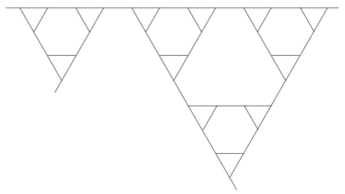
Figure 4: The Pascal graph.

Example 2.14 (Pascal graph).

Consider the Pascal graph $\mathcal{P}$ [18], which is an infinite $3$-regular graph, see Figure 4. Its edges graph is the Sierpiński lattice $\mathcal{L}$, and as was shown by Quint [18], the spectrum $\sigma(-\Delta_{\mathcal{P}})$ of its Laplacian $-\Delta_{\mathcal{P}}$ is the union of a countable set and the Julia set of a certain polynomial (affinely) conjugated to $R_{\mathcal{T}}$. From this we deduce that

$$\dim_{H}(\sigma(-\Delta_{\mathcal{P}}))=\dim_{H}({\mathcal{J}}_{\mathcal{P}})=\dim_{H}({\mathcal{J}}_{\mathcal{L}})=\dim_{H}(\sigma(-\Delta_{\mathcal{L}})),$$

which we estimate in Theorem 1.4.

2.5 Spectrum of the Laplacian for infinite Sierpiński gaskets

We finally turn to the case of an infinite Sierpiński gasket $\mathcal{T}^{\infty}$. The Laplacian $\Delta_{\mathcal{T}^{\infty}}$ is an operator with a domain in $L^{2}(\mathcal{T}^{\infty},\mu^{\infty})$. Here $\mu^{\infty}$ is the natural measure on $\mathcal{T}^{\infty}$, whose restriction to $\mathcal{T}$ equals $\mu$, and such that any two isometric sets are of equal measure (see [31]).

Remark 2.10 applies almost identically also to the Sierpiński gasket case: $\mathcal{T}^{\infty}$ depends non-trivially on the choice of a sequence $\omega$ in its definition, and different sequences typically give rise to non-isometric gaskets, with the boundary of $\mathcal{T}^{\infty}$ empty if and only if $\omega$ is eventually constant [31, Lemma 5.1]. The spectrum $\sigma(-\Delta_{\mathcal{T}^{\infty}})$, however, is independent of $\omega$ (even if the spectral decomposition is not, see [31, Remarks 5.4] or [26, Proposition 1]). Using the notation

$$\mathcal{R}(z)=\lim_{n\to\infty}5^{n}(S_{-1,\mathcal{T}})^{n}(z),$$

we have the following result on the spectrum $\sigma(-\Delta_{\mathcal{T}^{\infty}})$.

Proposition 2.15 ([31, Theorem 4]).

The operator $-\Delta_{\mathcal{T}^{\infty}}$ is an unbounded self-adjoint operator from a dense domain in $L^{2}(\mathcal{T}^{\infty},\mu^{\infty})$ to $L^{2}(\mathcal{T}^{\infty},\mu^{\infty})$. Its spectrum is $\sigma(-\Delta_{\mathcal{T}^{\infty}})=\mathcal{J}^{\infty}\cup\Sigma_{3}^{\infty}$ with

$$\mathcal{J}^{\infty}=\bigcup_{n=-\infty}^{\infty}5^{n}\mathcal{R}(\mathcal{J}_{\mathcal{T}})\quad\hbox{ and }\quad\Sigma_{3}^{\infty}=\bigcup_{n=-\infty}^{\infty}5^{n}\mathcal{R}(\Sigma_{3}),$$

where $\Sigma_{3}=\bigcup_{n=0}^{\infty}R^{-n}(\{3\})$.

A number of generalizations of this result for other unbounded nested fractals have been proved, see e.g. [25, 27]. The proposition immediately yields the following corollary.

Corollary 2.16.

We have that $\dim_{H}(\sigma(-\Delta_{\mathcal{T}^{\infty}}))=\dim_{H}(\mathcal{J}_{\mathcal{T}})$.

Thus estimating the Hausdorff dimension of the spectrum $\sigma(-\Delta_{\mathcal{T}^{\infty}})$ is again equivalent to estimating the Hausdorff dimension of the Julia set $\mathcal{J}_{\mathcal{T}}$.

3 Related results for other gaskets and lattices

In this section we describe other examples of fractal sets to which the same approach can be applied. In practice the computations may be more complicated, but the same basic method still applies.

3.1 Higher-dimensional infinite Sierpiński gaskets

Let $d\geqslant 2$ and $T_{i}\colon\mathbb{R}^{d}\to\mathbb{R}^{d}$ be contractions defined by

$$T_{i}(x_{1},\ldots,x_{d})=\left(\frac{x_{1}}{2},\ldots,\frac{x_{d}}{2}\right)+\frac{1}{2}e_{i},\quad\hbox{ for }i=1,\ldots,d,$$

where $e_{i}$ is the $i$th coordinate vector. The $d$-dimensional Sierpiński gasket $\mathcal{T}^{d}\subset\mathbb{R}^{d}$ is the smallest non-empty closed set such that

$$\mathcal{T}^{d}=\bigcup_{i=1}^{d}T_{i}(\mathcal{T}^{d}).$$

In [21], the analogous results are presented for the spectrum of the Laplacian $\Delta_{\mathcal{T}^{d}}$ associated to the corresponding Sierpiński gasket $\mathcal{T}^{d}\subset\mathbb{R}^{d}$ in $d$ dimensions $(d\geqslant 3$).

Definition 3.1.

For a sequence $(\omega_{n})_{n\in\mathbb{N}}\subset\{1,\ldots,d\}^{\mathbb{N}}$ we can define an infinite Sierpiński gasket in $d$ dimensions as

$$\mathcal{T}^{d,\infty}=\bigcup_{n=1}^{\infty}T_{\omega_{1}}^{-1}\circ\cdots\circ T_{\omega_{n}}^{-1}(\mathcal{T}^{d}).$$

As before, we can associate a Julia set ${\mathcal{J}}_{\mathcal{T}^{d}}$ and consider its Hausdorff dimension $\dim_{H}({\mathcal{J}}_{\mathcal{T}^{d}})$. More precisely, in each case, we can consider the decimation polynomial $R_{\mathcal{T}^{d}}\colon[0,3+d]\to\mathbb{R}$ defined by

$$R_{\mathcal{T}^{d}}(x)=x((3+d)-x),$$

with two local inverses $S_{\pm 1,\mathcal{T}^{d}}\colon[0,3+d]\to[0,3+d]$ given by

$$S_{\epsilon,\mathcal{T}^{d}}(x)=\frac{1}{2}\left(3+d+\epsilon\sqrt{9+6d+d^{2}-4x}\right)\quad\hbox{ with }\epsilon=\pm 1.$$

Let ${\mathcal{J}}_{\mathcal{T}^{d}}\subset[0,3+d]$ be the limit set of these two contractions, i.e., the smallest non-empty closed set such that

$${\mathcal{J}_{\mathcal{T}^{d}}}=S_{-1,\mathcal{T}^{d}}({\mathcal{J}}_{\mathcal{T}^{d}})\cup S_{+1,\mathcal{T}^{d}}({\mathcal{J}}_{\mathcal{T}^{d}}).$$

Theorem 3.2.

The Hausdorff dimension $\dim_{H}(\mathcal{J}_{\mathcal{T}^{d}})$ of the Julia set $\mathcal{J}_{\mathcal{T}^{d}}$ for $d\in\{2,\ldots,10\}$ associated to the Sierpiński gasket in $d$ dimensions is given by the values in Table 1, accurate to the number of decimals stated.

$d$	$\dim_{H}({\mathcal{J}}_{\mathcal{T}^{d}})$
2	0.55161856837246 …
3	0.45183750018171 …
4	0.39795943979056 …
5	0.36287714809375 …
6	0.33770271892130 …
7	0.31850809575800 …
8	0.30324865557723 …
9	0.29074069840192 …
10	0.28024518050407 …

Table 1: The Hausdorff dimension of ${\mathcal{J}}_{\mathcal{T}^{d}}$ for $2\leqslant d\leqslant 10$.

The proof uses the same algorithmic method as that of Theorem 1.4, see Section 4.

Remark 3.3.

By arguments developed in [9] and [26], one can deduce that similarly to Proposition 2.15 and Corollary 2.16, the Hausdorff dimensions of the spectrum of the appropriately defined Laplacian on $\mathcal{T}^{d,\infty}$ and the Julia set $\dim_{H}({\mathcal{J}}_{\mathcal{T}^{d}})$ coincide.

We can observe empirically from the table that the dimension decreases as $d\to+\infty$. The following simple lemma confirms that $\lim_{d\to+\infty}\dim_{H}(\mathcal{J}_{\mathcal{T}^{d}})=0$ with explicit bounds.

Lemma 3.4.

As $d\to+\infty$ we can bound

$$\frac{\log 2}{\log(d+3)}\leqslant\dim_{H}(\mathcal{J}_{\mathcal{T}^{d}})\leqslant\frac{2\log 2}{\log(d+3)+\log(d-1)}.$$

Proof.

We can write

$$I_{1}:=R_{\mathcal{T}^{d}}^{-1}([0,3+d])\cap\left[0,\frac{3+d}{2}\right]=\left[0,\frac{3+d}{2}\left(1-\sqrt{1-\frac{4}{3+d}}\right)\right].$$

Thus for $x\in I_{1}$ we have bounds

$$\sqrt{(3+d)(d-1)}\leqslant|R_{\mathcal{T}^{d}}^{\prime}(x)|\leqslant 3+d.$$

Similarly, we can define $I_{2}:=R_{\mathcal{T}^{d}}^{-1}([0,3+d])\cap\left[\frac{3+d}{2},3+d\right]$ and obtain the same bounds on $|R_{\mathcal{T}^{d}}^{\prime}(x)|$ for $x\in I_{2}$. In particular, we can then bound

$$\frac{\log 2}{\log(3+d)}\leqslant\dim_{H}(\mathcal{J}_{\mathcal{T}^{d}})\leqslant\frac{2\log 2}{\log(3+d)+\log(d-1)}.\qed$$

3.2 Post-critically finite self-similar sets

The method of spectral decimation used for the Sierpiński gasket by Fukushima and Shima [9], was extended by Shima [28] to post-critically finite self-similar sets and thus provided a method for analyzing the spectra of their Laplacians.

Definition 3.5.

Let $\Sigma=\{1,\ldots,k\}^{\mathbb{Z}_{+}}$ be the space of (one-sided) infinite sequences with the Tychonoff product topology, and $\sigma$ the usual left-shift map on $\Sigma$.

Let $T_{1},\ldots,T_{k}\colon\mathbb{R}^{d}\to\mathbb{R}^{d}$ be contracting similarities and let $\mathcal{X}$ be the limit set, i.e., the smallest closed subset with $\mathcal{X}=\bigcup_{i=1}^{k}T_{i}(\mathcal{X})$. Let $\pi\colon\Sigma\to\mathcal{X}$ be the natural continuous map defined by

$$\pi\left((w_{n})_{n=0}^{\infty}\right)=\lim_{n\to+\infty}T_{w_{0}}T_{w_{1}}\cdots T_{w_{n}}(0).$$

We say that $\mathcal{X}$ is post-critically finite if

$$\#\left(\bigcup_{n=0}^{\infty}\sigma^{n}\left\{(w_{n})\in\Sigma:\pi(w_{n})\in K\right\}\right)<+\infty$$

where $K=\bigcup_{i\neq j}T_{i}\mathcal{X}\cap T_{j}\mathcal{X}$.

         

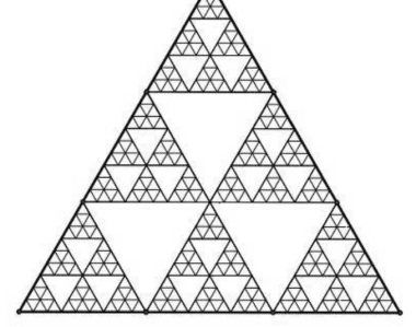
Figure 5: The first two graphs for $SG_{3}$ (left, centre) and the $SG_{3}$ gasket (right).

         

Figure 6: The function $R_{SG_{3}}(x)$ and the four contracting inverse branches for the $SG_{3}$ gasket.

The original Sierpiński triangle $\mathcal{T}$ is an example of a limit set which is post-critically finite. So is the following variant on the Sierpiński triangle.

Example 3.6 ($SG_{3}$ gasket).

We can consider the Sierpiński gasket $SG_{3}$ (see Figure 5) which is the smallest non-empty closed set $\mathcal{X}_{SG_{3}}$ such that $\mathcal{X}_{SG_{3}}=\bigcup_{i=1}^{6}T_{i}\mathcal{X}_{SG_{3}}$ where

$$T_{j}(x,y)=p_{j}+\left(\frac{x}{3},\frac{y}{3}\right)\quad\hbox{ for }j=1,\ldots,6,$$

with

$$p_{1}=(0,0),p_{2}=\left(\frac{1}{3},0\right),p_{3}=\left(\frac{2}{3},0\right),p_{4}=\left(\frac{1}{6},\frac{1}{2\sqrt{3}}\right),p_{5}=\left(\frac{1}{2},\frac{1}{2\sqrt{3}}\right),p_{6}=\left(\frac{1}{3},\frac{1}{\sqrt{3}}\right).$$

In this case we can associate the decimation rational function $R_{SG_{3}}\colon[0,6]\to[0,6]$ given by

$$R_{SG_{3}}(x)=\frac{3x(5-x)(4-x)(3-x)}{14-2x},$$

for which there are four local inverses $S_{j,SG_{3}}$ (for $j=1,2,3,4$) [7], see Figure 6. The associated Julia set ${\mathcal{J}}_{SG_{3}}$, which is the smallest non-empty closed set such that ${\mathcal{J}}_{SG_{3}}=\bigcup_{j=1}^{4}S_{j,SG_{3}}({\mathcal{J}}_{SG_{3}})$, has Hausdorff dimension $\dim_{H}({\mathcal{J}}_{SG_{3}})$.

Using Mathematica with a sufficiently high precision setting (see Example 4.4 for more details) we can numerically compute the Hausdorff dimension of the Julia set ${\mathcal{J}}_{SG_{3}}$ associated to the Sierpiński gasket $SG_{3}$ to be

$$\dim_{H}({\mathcal{J}}_{SG_{3}})=0.617506301862352229042494874316407096341976\ldots$$

Example 3.7 (Vicsek graph).

The Vicsek set $X_{\mathcal{V}}$ is the smallest non-empty closed set such that $X_{\mathcal{V}}=\bigcup_{j=1}^{5}T_{j}(X_{\mathcal{V}})$ where

$$T_{j}(x,y)=p_{j}+\left(\frac{x}{3},\frac{y}{3}\right)\quad\hbox{ for }j=1,\ldots,5,$$

with

$$p_{1}=(0,0),~{}p_{2}=\left(\frac{2}{3},0\right),~{}p_{3}=\left(\frac{2}{3},\frac{2}{3}\right),~{}p_{4}=\left(0,\frac{2}{3}\right),~{}p_{5}=\left(\frac{1}{3},\frac{1}{3}\right).$$

In this case, studied in [20, Example 6.3], one has that $R_{\mathcal{V}}\colon[-1,0]\to\mathbb{R}$ is given by

$$R_{\mathcal{V}}(z)=z(6z+3)(6z+5),$$

with three inverse branches $S_{1},S_{2},S_{3}\colon[-1,0]\to[-1,0]$ given by

$$S_{1}(x) =\frac{1}{36}\left(i(\sqrt{3}+i)t(x)-\frac{19(1+i\sqrt{3})}{t(x)}-16\right),$$

$$S_{2}(x) =\frac{1}{36}\left(-i(\sqrt{3}-i)t(x)-\frac{19(1-i\sqrt{3})}{t(x)}-16\right),$$

$$S_{3}(x) =\frac{1}{18}\left(t(x)+\frac{19}{t(x)}-8\right),$$

where $t(x)=\left(9\cdot(81x^{2}+56x-75)^{1/2}+81x+28\right)^{1/3}$. The associated Julia set ${\mathcal{J}}_{\mathcal{V}}$ is the smallest non-empty closed set such that ${\mathcal{J}}_{\mathcal{V}}=\bigcup_{j=1}^{3}S_{j,\mathcal{V}}({\mathcal{J}}_{\mathcal{V}})$. The following theorem is proved similarly to Theorem 1.4, as described in Section 4.

Theorem 3.8.

The Hausdorff dimension of the Julia set ${\mathcal{J}}_{\mathcal{V}}$ is

$$\dim_{H}({\mathcal{J}}_{\mathcal{V}})=0.49195457005266\ldots,$$

accurate to the number of decimals stated.

Remark 3.9.

Analogously to the case of the Sierpiński lattice $\mathcal{L}$, we can define lattices $\mathcal{L}_{SG_{3}}$ and $\mathcal{L}_{\mathcal{V}}$ for the $SG_{3}$ and Vicsek sets from the previous two examples, as well as corresponding graph Laplacians $\Delta_{\mathcal{L}_{SG_{3}}}$ and $\Delta_{\mathcal{L}_{\mathcal{V}}}$. The Hausdorff dimensions of their spectra can again be directly related to those of the respective Julia sets $\mathcal{J}_{SG_{3}}$ and $\mathcal{J}_{\mathcal{V}}$. By [20, Theorem 5.8], one has that ${\mathcal{J}}_{SG_{3}}\subseteq\sigma(-\Delta_{\mathcal{L}_{SG_{3}}})\subseteq{\mathcal{J}}_{SG_{3}}\cup\mathcal{D}_{SG_{3}}$ and ${\mathcal{J}}_{\mathcal{V}}\subseteq\sigma(-\Delta_{\mathcal{L}_{\mathcal{V}}})\subseteq{\mathcal{J}}_{\mathcal{V}}\cup\mathcal{D}_{\mathcal{V}}$, where $\mathcal{D}_{SG_{3}}$ and $\mathcal{D}_{\mathcal{V}}$ are countable sets. It follows, analogously to Corollary 2.13, that $\dim_{H}(\sigma(-\Delta_{\mathcal{L}_{SG_{3}}}))=\dim_{H}({\mathcal{J}}_{SG_{3}})$ and $\dim_{H}(\sigma(-\Delta_{\mathcal{L}_{\mathcal{V}}}))=\dim_{H}({\mathcal{J}}_{\mathcal{V}})$.

Remark 3.10.

Other examples to which the same method could be applied include the modified Koch curve (see [19], [15]) for which the associated rational function is $R(x)=9x(x-1)(x-\frac{4}{3})(x-\frac{5}{3})/(x-\frac{3}{2}).$ More families of such examples can be found in [32].

Remark 3.11.

The spectral decimation method can also apply to some non-post-critically finite examples, such as the diamond fractal [14], for which the associated polynomial is $R(x)=2x(2+x)$. On the other hand, there are symmetric fractal sets which do not admit spectral decimation, such as the pentagasket, as studied in [1].

4 Dimension estimate algorithm for Theorem 1.4

This section is dedicated to finishing the proof of Theorem 1.4, by describing an algorithm yielding estimates (with rigorous error bounds) for the values of the Hausdorff dimension.

By the above discussion we have reduced the estimation of the Hausdorff dimensions of $\sigma(-\Delta_{\mathcal{L}})$ and $\sigma(-\Delta_{\mathcal{T}^{\infty}})$ to that of $\dim_{H}({\mathcal{J}}_{\mathcal{T}})$ for the limit set ${\mathcal{J}}_{\mathcal{T}}$ associated to $S_{\pm 1,\mathcal{T}}$ from (2.4) (and similarly for the other examples). Unfortunately, since the maps $S_{\pm 1,\mathcal{T}}$ are non-linear it is not possible to give an explicit closed form for the value $\dim_{H}(\sigma(-\Delta_{\mathcal{T}}))=\dim_{H}({\mathcal{J}}_{\mathcal{T}})$. Recently developed simple methods make the numerical estimation of this value relatively easy to implement, which we summarize in the following subsections.

4.1 A functional characterization of dimension

Let $\mathcal{B}=C(I)$ be the Banach space of continuous functions on the interval $I=[0,5]$ with the norm $\|f\|_{\infty}=\sup_{x\in I}|f(x)|$.

Definition 4.1.

Let $\mathcal{L}_{t}$ (for $t\geqslant 0$) be the transfer operator defined by

$$\mathcal{L}_{t}f(x)=|S_{-1,\mathcal{T}}^{\prime}(x)|^{t}f(S_{-1,\mathcal{T}}(x))+|S_{+1,\mathcal{T}}^{\prime}(x)|^{t}f(S_{+1,\mathcal{T}}(x))$$

where $f\in\mathcal{B}\hbox{ and }x\in I$, and $S_{\pm,\mathcal{T}}$ are as in (2.4).

It is well known that the transfer operator $\mathcal{L}_{t}$ (for $t\geqslant 0$) is a well-defined positive bounded operator from $\mathcal{B}$ to itself. To make use of the results in the previous sections, we employ the following “min-max method” result:

Lemma 4.2 ([17]).

Given choices of $0<t_{0}<t_{1}<1$ and strictly positive continuous functions $f,g\colon I\to\mathbb{R}^{+}$ with

$$\inf_{x\in I}\frac{\mathcal{L}_{t_{0}}f(x)}{f(x)}>1\quad\hbox{ and }\quad\sup_{x\in I}\frac{\mathcal{L}_{t_{1}}g(x)}{g(x)}<1,$$ (4.1)

then $t_{0}<\dim_{H}({\mathcal{J}}_{\mathcal{T}})<t_{1}$.

Proof.

We briefly recall the proof. We require the following standard properties.

1. For any $t\geqslant 0$ the operator $\mathcal{L}_{t}$ has a maximal positive simple eigenvalue $e^{P(t)}$ (with positive eigenfunction), where $P$ is the pressure function [23, 16].

2. $P\colon\mathbb{R}^{+}\to\mathbb{R}$ is real analytic and convex [23].

3. The value $t=\dim(\mathcal{J}_{\mathcal{T}})$ is the unique solution to $P(t)=0$, see [5, 24].

By property 1. and the first inequality in (4.1) we can deduce that

$$P(t_{0})=\lim_{n\to+\infty}\frac{1}{n}\log\|\mathcal{L}_{t_{0}}^{n}f\|_{\infty}>0.$$ (4.2)

By property 1. and the second inequality in (4.1) we can deduce that

$$P(t_{1})=\lim_{n\to+\infty}\frac{1}{n}\log\|\mathcal{L}_{t_{1}}^{n}g\|_{\infty}<0.$$ (4.3)

Comparing properties 2. and 3. with (4.2) and (4.3), the result follows. ∎

4.2 Rigorous verification of minmax inequalities

Next, we explain how we rigorously verify the conditions of Lemma 4.2 for a function $f\colon I\to\mathbb{R}^{+}$, that is,

1. $f>0$,

2. $\inf_{x\in I}h(x)>1$ or $\sup_{x\in I}h(x)<1$ for $h(x):=(\mathcal{L}_{t}f)(x)/f(x)$.

In order to obtain rigorous results we make use of the arbitrary precision ball arithmetic library Arb [11], which for a given interval $[c-r,c+r]$ and function $f$ outputs an interval $[c^{\prime}-r^{\prime},c^{\prime}+r^{\prime}]$ such that $f([c-r,c+r])\subseteq[c^{\prime}+r^{\prime},c^{\prime}-r^{\prime}]$ is guaranteed. Clearly, the smaller the size of the input interval, the tighter the bounds on its image. Thus, in order to verify the above conditions we partition the interval $I$ adaptively using a bisection method up to depth $k\in\mathbb{N}_{0}$ into at most $2^{k}$ subintervals, and check these conditions on each subinterval. While the first condition is often immediately satisfied for chosen test functions $f$ on the whole interval $I$, the second condition is much harder to check as $h$ is very close to $1$ and would require very large depth $k$.

To counteract the exponential growth of the number of required subintervals, we use tighter bounds on the image of $h$. Clearly for $x\in[c-r,c+r]$ with $c\in\mathbb{R}$ and $r>0$, we have that $|h(x)-h(c)|\leqslant\sup_{y\in[c-r,c+r]}|h^{\prime}(y)|r$ by the mean value theorem. More generally, we obtain for $p\in\mathbb{N}$ that

$$|h(x)-h(c)|\leqslant\sum_{i=1}^{p-1}|h^{(i)}(c)|r^{i}+\sup_{y\in[c-r,c+r]}|h^{(p)}(y)|r^{p}.$$

This allows to achieve substantially tighter bounds on $h([c-r,c+r])$ while using a moderate number of subintervals, at the cost of additionally computing the first $p$ derivatives of $h$.

4.3 Choice of $f$ and $g$ via an interpolation method

Here we explain how to choose suitable functions $f$ and $g$ for use in Lemma 4.2, so that given candidate values $t_{0}<t_{1}$ we can confirm that $t_{0}<\dim_{H}({\mathcal{J}}_{\mathcal{T}})<t_{1}$. Clearly, if $f$ and $g$ are eigenfunctions of $\mathcal{L}_{t_{0}}$ and $\mathcal{L}_{t_{1}}$ for the eigenvalues $\lambda_{t_{0}}$ and $\lambda_{t_{1}}$, respectively, then condition (4.2) is easy to check. As these eigenfunctions are not known explicitly, we will use the Lagrange-Chebyshev interpolation method to approximate the respective transfer operators by finite-rank operators of rank $m$, and thus obtain approximations $f^{(m)}$ and $g^{(m)}$ of $f$ and $g$. As the maps $S_{\pm 1,\mathcal{T}}$ involved in the definition of the transfer operator (Definition 4.1) extend to holomorphic functions on suitable ellipses, Theorem 3.3 and Corollary 3 of [3] guarantee that the (generalized) eigenfunctions of the finite-rank operator converge (in supremum norm) exponentialy fast in $m$ to those of the transfer operator. In particular, for large enough $m$ the functions $f^{(m)}$ and $g^{(m)}$ are positive on the interval $I$ and are good candidates for Lemma 4.2.

Initial choice of $m$. We first make an initial choice of $m\geqslant 1$. Let $\ell_{n}\colon I\to\mathbb{R}$ (for $n=0,\ldots,m-1$) denote the Lagrange polynomials scaled to $[0,5]$ and let $x_{n}\in[0,5]$ (for $n=0,\ldots,m-1$) denote the associated Chebyshev points.

Initial construction of test functions. Let $v^{t}=(v_{i}^{t})_{i=0}^{m-1}$ be the left eigenvector for the maximal eigenvalue of the $m\times m$ matrix $M_{t}(i,j)=(\mathcal{L}_{t}\ell_{i})(x_{j})$ (for $0\leqslant i,j\leqslant m-1$) and set

$$f^{(m)}:=\sum_{i=0}^{m-1}v_{i}^{t_{0}}\ell_{i}\quad\hbox{ and }\quad g^{(m)}:=\sum_{i=0}^{m-1}v_{i}^{t_{1}}\ell_{i}.$$

If the choices $f=f^{(m)}$ and $g=g^{(m)}$ satisfy the hypotheses of Lemma 4.2 (which can be checked rigorously with the method in the previous section) then we proceed to the next step. If they do not, we increase $m$ and try again.

Conclusion. When the hypothesis of Lemma 4.2 holds then its assertion confirms that $t_{0}<\dim_{H}(\mathcal{J}_{\mathcal{T}})<t_{1}$.

It remains to iteratively make the best possible choices of $t_{0}<t_{1}$ using the following approach.

4.4 The bisection method

Fix $\epsilon>0$. We can combine the above method of choosing $f$ and $g$ with a bisection method to improve given lower and upper bounds $t_{0}$ and $t_{1}$ until the latter are $\epsilon$-close:

Initial choice. First we can set $t_{0}^{(1)}=0$ and $t_{1}^{(1)}=1$, for which $t_{0}^{(1)}<\dim_{H}(\mathcal{J}_{\mathcal{T}})<t_{1}^{(1)}$ is trivially true.

Iterative step. Given $n\geqslant 0$ we assume that we have chosen $t_{0}^{(n)}<t_{1}^{(n)}$. We can then set $T=(t_{0}^{(n)}+t_{1}^{(n)})/2$ and proceed as follows.

1. If $t_{0}^{(n)}<\dim_{H}(\mathcal{J}_{\mathcal{T}})<T$ then set $t_{0}^{(n+1)}=t_{0}^{(n)}$ and $t_{1}^{(n+1)}=T$.

2. If $T<\dim_{H}(\mathcal{J}_{\mathcal{T}})<t_{1}^{(n)}$ then set $t_{0}^{(n+1)}=T$ and $t_{1}^{(n+1)}=t_{1}^{(n)}$.

3. If $\dim_{H}(\mathcal{J}_{\mathcal{T}})=T$ then we have the final value.

Final choice. Once we arrive at $t_{1}^{(n)}-t_{0}^{(n)}<\epsilon$ then we can set $t_{0}=t_{0}^{(n)}$ and $t_{1}=t_{1}^{(n)}$ as the resulting upper and lower bounds for the true value of $\dim_{H}(\mathcal{J}_{\mathcal{T}})$.

Applying this algorithm yields the proof of Theorem 1.4 (and with the obvious modifications also those of Theorems 3.2 and 3.8). Specifically, we computed the value of $\dim_{H}(\mathcal{J}_{\mathcal{T}})$ efficiently to the $14$ decimal places as stated with the above method, by setting $\epsilon=10^{-15}$, using finite-rank approximation up to rank $m=30$, running interval bisections for rigorous minmax inequality verification up to depth $k=18$, i.e. using up to $2^{18}$ subintervals, and using $p=2$ derivatives. There are of course many ways to improve accuracy further, e.g., with more computation or the use of higher derivatives.

Example 4.3 (Sierpiński triangle).

To cheaply obtain a more accurate estimate (albeit without the rigorous guarantee resulting from the use of ball arithmetic), we use the MaxValue routine from Mathematica. To get an estimate on $\dim_{H}({\mathcal{J}}_{\mathcal{T}})$ to $60$ decimal places, we work with $100$ decimal places as Mathematica’s precision setting. Taking $m=60$ we use the bisection method and starting from an interval $[0.2,0.8]$ after $199$ iterations we have upper and lower bounds $t_{0}\leqslant\dim_{H}({\mathcal{J}}_{\mathcal{T}})\leqslant t_{1}$, where

$$t_{0}= 0.5516185683724609316975708723135206545360797417440422$$

$$\qquad 0826629\color[rgb]{.5,.5,.5}$$

and

$$t_{1}= 0.5516185683724609316975708723135206545360797417440422$$

$$\qquad 0826629\color[rgb]{.5,.5,.5}.$$

With a little more computational effort ($200$ decimals of precision, $m=100$, $329$ iterations) we can improve the estimate to $100$ decimal places:

$$t_{0}= 0.55161856837246093169757087608456543417211766450713$$

$$\quad 8868116831699168666814224190486583439508658139692\color[rgb]{.5,.5,.5}$$

$$\quad\color[rgb]{.5,.5,.5}$$

$$\quad\color[rgb]{.5,.5,.5}$$

and

$$t_{1}= 0.55161856837246093169757087608456543417211766450713$$

$$\quad 8868116831699168666814224190486583439508658139692\color[rgb]{.5,.5,.5}$$

$$\quad\color[rgb]{.5,.5,.5}$$

$$\quad\color[rgb]{.5,.5,.5},$$

which yields the estimate:

$$\dim_{H}(\mathcal{J}_{\mathcal{T}})=0.5516185683724609316975708760845654341721176$$

$$\quad 6450718868116831699168666814224190486583439508658139692\ldots.$$

We next consider as a second example, $SG_{3}$, see Example 3.6.

Example 4.4 ($SG_{3}$ gasket).

With the same method as in the previous example, we estimate bounds on $\dim_{H}({\mathcal{J}}_{SG_{3}})$ to $60$ decimal places:

$$t_{0}= 0.6175063018623522290424948743164070963419768663609616$$

$$\qquad 0395161\color[rgb]{.5,.5,.5}$$

and

$$t_{1}= 0.6175063018623522290424948743164070963419768663609616$$

$$\qquad 0395161\color[rgb]{.5,.5,.5},$$

which yields the estimate:

$$\dim_{H}({\mathcal{J}}_{SG_{3}}) =0.617506301862352229042494874316$$

$$\qquad 40709634197686636096160395161\ldots$$

Remark 4.5.

A significant contribution to the time complexity of the algorithm is that of estimating the top eigenvalue and corresponding eigenvector of an $m\times m$ matrix which is $O(n\cdot m^{2})$ with $n$ denoting the number of steps of the power iteration method. Moreover, by perturbation theory one might expect that in order to get an error in the eigenvector of $\epsilon>0$ one needs to choose $m=O(\log(1/\epsilon))$ and $n=O(\log(1/\epsilon))$.

5 Conclusion

In this note, we have leveraged the existing theory on Laplacians associated to Sierpiński lattices, infinite Sierpiński gaskets and other post-critically finite self-similar sets, in order to establish the Hausdorff dimensions of their respective spectra. We used the insight that, by virtue of the iterative description of these spectra, these dimensions coincide with those of the Julia sets of certain rational functions. Since the contractive local inverse branches of these functions are non-linear, the values of the Hausdorff dimensions are not available in an explicit closed form, in contrast to the dimensions of the (infinite) Sierpiński gaskets themselves, or other self-similar fractals constructing using contracting similarities and satisfying an open set condition. Therefore we use the fact that the Hausdorff dimension can be expressed implicitly as the unique zero of a so-called pressure function, which itself corresponds to the maximal positive simple eigenvalue of a family of positive transfer operators. Using a min-max method combined with the Lagrange-Chebyshev interpolation scheme we can rigorously estimate the leading eigenvalues for every operator in this family. Combined with a bisection method we then accurately and efficiently estimate the zeros of the respective pressure functions, yielding rigorous and effective bounds on the Hausdorff dimensions of the spectra of the relevant Laplacians.

M. Pollicott, Department of Mathematics, University of Warwick, Coventry, CV4 7AL, UK.

E-mail: masdbl@warwick.ac.uk

J. Slipantschuk, Department of Mathematics, University of Warwick, Coventry, CV4 7AL, UK.

E-mail: julia.slipantschuk@warwick.ac.uk

References

- [1] B. Adams, S.A. Smith, R.S. Strichartz, A. Teplyaev, The spectrum of the Laplacian on the pentagasket, Fractals in Graz 2001, 1–24, Trends Math., Birkhäuser, Basel, 2003.
- [2] S. Alexander, Some properties of the spectrum of the Sierpiński gasket in a magnetic field, Phys. Rev. B 29 (1984) 5504–5508.
- [3] O.F. Bandtlow and J. Slipantschuk, Lagrange approximation of transfer operators associated with holomorphic data, (2020) Preprint: arXiv:2004.03534.
- [4] J. Béllissard, Renormalization group analysis and quasicrystals, Ideas and methods in quantum and statistical physics (Oslo, 1988), 118–148, Cambridge Univ. Press, Cambridge, 1992.
- [5] R. Bowen, Hausdorff dimension of quasi-circles, Publ. Math. I.H.E.S. 50 (1979) 11–25.
- [6] N. Cohen, Fractal Antennas Part 1: Introduction and the Fractal Quad, Communications Quarterly 5 (1995) 7–22.
- [7] S. Drenning and R. Strichartz, Spectral decimation on Hambley’s homogeneous hierarchical gaskets, Illinois J. Math. 53 (2009) 915–937.
- [8] K. Falconer, Fractal Geometry, Addison-Wesley, 2003.
- [9] M. Fukushima and T. Shima, On a spectral analysis for the Sierpiński gasket, Potential Anal. 1 (1992) 1–35.
- [10] R. Hohlfeld, N. Cohen, Self-similarity and the geometric requirements for frequency independence in antennae, Fractals 7 (1999) 79–84.
- [11] F. Johansson, Arb: Efficient arbitrary-precision midpoint-radius interval arithmetic, IEEE Trans. Comput. 66 (2017) 1281–1292.
- [12] J. Kigami, Analysis on Fractals, Cambridge Tracts in Mathematics 143, Cambridge Univ. Press, Cambridge, 2008.
- [13] J. Kigami, A harmonic calculus on the Sierpinski spaces, Japan J. Appl. Math. 8 (1989) 259–290.
- [14] J. Kigami, R.S. Strichartz, K.C. Walker, Constructing a Laplacian on the diamond fractal, Experiment. Math. 10 (2001) 437–448.
- [15] L. Malozemov, Spectral theory of the differential Laplacian on the modified Koch curve, Geometry of the Spectrum (Seattle, WA, 1993), Contemp. Math. 173, Amer. Math. Soc., Providence, RI, 1994, 193–224.
- [16] W. Parry and M. Pollicott, Zeta functions and the periodic orbit structure of hyperbolic dynamics, Astérisque 187-188 (1990) 1–256.
- [17] M. Pollicott and P. Vytnova, Hausdorff dimension estimates applied to Lagrange and Markov spectra, Zaremba theory, and limit sets of Fuchsian groups, Trans. Amer. Math. Soc., to appear.
- [18] J.-F. Quint, Harmonic analysis on the Pascal graph, J. Funct. Anal. 256 (2009) 3409–3460.
- [19] L. Malozemov and A. Teplyaev, Pure point spectrum of the Laplacians on fractal graphs, J. Funct. Anal. 129 (1995) 390–405.
- [20] L. Malozemov and A. Teplyaev, Self-similarity, operators and dynamics, Math. Phys. Anal. Geom. 6 (2003) 201–218.
- [21] R. Rammal, Spectrum of harmonic excitations on fractals, J. Phys. 45 (1984) 191–206.
- [22] R. Rammal and G. Toulouse, Random walks on fractal structures and percolation clusters, J. Phys. Lett. 44 (1983) 13–22.
- [23] D. Ruelle, Thermodynamic Formalism, Addison-Wesley, New York, 1978.
- [24] D. Ruelle, Repellers for real analytic maps, Ergodic Theory Dynam. Systems, 2 (1982) 99–107.
- [25] C. Sabot, Pure point spectrum for the Laplacian on unbounded nested fractals, J. Funct. Anal. 173 (2000) 497–524.
- [26] C. Sabot, Laplace operators on fractal lattices with random blow-ups, Potential Anal. 20 (2004) 177–193.
- [27] R. Strichartz and A. Teplyaev, Spectral analysis on infinite Sierpiński fractafolds, J. Anal. Math. 116 (2012) 255–297.
- [28] T. Shima, On eigenvalue problems for Laplacians on p.c.f. self-similar sets, Japan J. Indust. Appl. Math. 13 (1996) 1–23.
- [29] R. Strichartz, Analysis on Fractals, Notices Amer. Math. Soc. 46 (1999) 1199–1208.
- [30] R. Strichartz, Differential Equations on Fractals: A Tutorial, Princeton University Press, Princeton, 2006.
- [31] A. Teplyaev, Spectral analysis on infinite Sierpiński gaskets, J. Funct. Anal. 159 (1998) 537–567.
- [32] A. Teplyaev, Harmonic coordinates on fractals with finitely ramified cell structure, Canad. J. Math. 60 (2008) 457–480.