Attribution-Scores in Data Management and Explainable Machine Learning

Abstract

We describe recent research on the use of actual causality in the definition of responsibility scores as explanations for query answers in databases, and for outcomes from classification models in machine learning. In the case of databases, useful connections with database repairs are illustrated and exploited. Repairs are also used to give a quantitative measure of the consistency of a database. For classification models, the responsibility score is properly extended and illustrated. The efficient computation of Shap-score is also analyzed and discussed. The emphasis is placed on work done by the author and collaborators.

1 Introduction

In data management and artificial intelligence, and machine learning in particular, one wants explanations for certain results. For example, for query answers and inconsistency in databases. In machine learning (ML), one wants explanations for automated classification results, and automated decision making. Explanations, that may come in different forms, have been the subject of philosophical enquires for a long time, but, closer to our discipline, they appear under different forms in model-based diagnosis, and in causality as developed in artificial intelligence.

In the last few years, explanations that are based on numerical scores assigned to elements of a model that may contribute to an outcome have become popular. These attribution scores attempt to capture the degree of contribution of those components to an outcome, e.g. answering questions like these: What is the contribution of this tuple to the answer to this query? Or, what is the contribution of this feature value for the label assigned to this input entity?

In this article, we survey some of the recent advances on the definition, use and computation of the above mentioned score-based explanations for query answering in databases, and for outcomes from classification models in ML. This is not intended to be an exhaustive survey of the area. Instead, it is heavily influenced by our latest research. To introduce the concepts and techniques we will use mostly examples, trying to convey the main intuitions and issues.

Different scores have been proposed in the literature, and some that have a relatively older history have been applied. Among the latter we find the general responsibility score as found in actual causality [24, 19, 25]. For a particular kind of application, one has to define the right causality setting, and then apply the responsibility measure to the participating variables.

In data management, responsibility has been used to quantify the strength of a tuple as a cause for a query result [36, 7].  The responsibility score, ${\it Resp}$, is based on the notions of counterfactual intervention as appearing in actual causality. More specifically, (potential) executions of counterfactual interventions on a structural logico-probabilistic model  [24] are considered, with the purpose of answering hypothetical questions of the form:  What would happen if we change …?.

Database repairs are commonly used to define and obtain semantically correct query answers from a database (DB) that may fail to satisfy a given set of integrity constraints (ICs) [6]. A connection between repairs and actual causality in DBs has been used to obtain complexity results and algorithms for responsibility [7] (see Section 2). Actual causality and responsibility can also be defined at the attribute-level in DBs (rather than at the tuple-level) [9]. We briefly describe this alternative in Section 2.1.  On the basis of database repairs, a measure (or global score) to quantify the degree of inconsistency of a DB was introduced in [8]. We give the main ideas in Section 3.

The Resp score has also been applied to define scores for binary attribute values in classification [11]. However, it has to be generalized when dealing with non-binary features [10]. We describe this generalization in Section 4.1.

The Shapley value of coalition game theory [44, 40] can be (and has been) used to define attribution scores, in particular in DBs. The main idea is that several tuples together, much like players in a coalition game, are necessary to produce a query result. Some may contribute more than others to the wealth distribution function (or simply, game function), which in this case becomes the query result, namely $1$ or $0$ if the query is Boolean, or a number in the case of an aggregation query. This use of Shapley value was developed in [30, 31]. See also [15] for a more recent and general discussion of the use of the Shapley value in DBs.

The Shapley value has also been used to define explanation scores to feature values in ML-based classification, taking the form of the Shap score [34]. Since its computation is bound to be intractable in general, there has been recent research on classes of models for which Shap becomes tractable [4, 5, 48]. See Section 4.2.

There hasn’t been much research on the use or consideration of domain knowledge (or domain semantics) in the definition and computation of attribution scores. In Section 5, we describe some problems that emerge in this context.

This article has [16] as a companion, which concentrates mostly on data management. It delves into the Resp score under ICs, and on the use of the Shapley value for query answering in DBs. That paper also discusses the Causal Effect score applied in data management [42]. It is also based on causality, as it appears mainly in observational studies [41, 26, 39].

2 Causal Responsibility in Databases

Before going into the subject, we recall some notions and notation used in data management.   A relational schema $\mathcal{R}$ contains a domain of constants, $\mathcal{C}$, and a set of predicates of finite arities, $\mathcal{P}$.  $\mathcal{R}$ gives rise to a language $\mathfrak{L}(\mathcal{R})$ of first-order (FO) predicate logic with built-in equality, $=$. Variables are usually denoted with $x,y,z,...$; and finite sequences thereof with $\bar{x},...$; and constants with $a,b,c,...$, etc. An atom is of the form $P(t_{1},\ldots,t_{n})$, with $n$-ary $P\in\mathcal{P}$ and $t_{1},\ldots,t_{n}$ terms, i.e. constants, or variables. An atom is ground (a.k.a. a tuple) if it contains no variables. A database (instance), $D$, for $\mathcal{R}$ is a finite set of ground atoms; and it serves as an interpretation structure for $\mathfrak{L}(\mathcal{R})$.

A conjunctive query (CQ) is a FO formula, $\mathcal{Q}(\bar{x})$, of the form  $\exists\bar{y}\;(P_{1}(\bar{x}_{1})\wedge\dots\wedge P_{m}(\bar{x}_{m}))$, with $P_{i}\in\mathcal{P}$, and (distinct) free variables $\bar{x}:=(\bigcup\bar{x}_{i})\smallsetminus\bar{y}$. If $\mathcal{Q}$ has $n$ (free) variables, $\bar{c}\in\mathcal{C}^{n}$  is an answer to $\mathcal{Q}$ from $D$ if $D\models\mathcal{Q}[\bar{c}]$, i.e. $Q[\bar{c}]$ is true in $D$ when the variables in $\bar{x}$ are componentwise replaced by the values in $\bar{c}$. $\mathcal{Q}(D)$ denotes the set of answers to $\mathcal{Q}$ from $D$. $\mathcal{Q}$ is a Boolean conjunctive query (BCQ) when $\bar{x}$ is empty; and when true in $D$, $\mathcal{Q}(D):=\{{\it true}\}$. Otherwise, it is false, and $\mathcal{Q}(D):=\emptyset$. We will consider only conjunctive queries, which are the most common the data management.

Integrity constraints (ICs) are sentences of $\mathfrak{L}(\mathcal{R})$ that a DB is expected to satisfy. Here, we consider mainly denial constraints  (DCs), i.e. of the form $\kappa\!:\neg\exists\bar{x}(P_{1}(\bar{x}_{1})\wedge\dots\wedge P_{m}(\bar{x}_{m}))$, where $P_{i}\in\mathcal{P}$, and $\bar{x}=\bigcup\bar{x}_{i}$.   If an instance $D$ does not satisfy the set $\Sigma$ of ICs associated to the schema, we say that $D$ is inconsistent, denoted with  $D\not\models\Sigma$.

Now we move into the proper subject of this section.   In data management we need to understand and compute why certain results are obtained or not, e.g. query answers, violations of semantic conditions, etc.; and we expect a database system to provide explanations.  Here, we will consider explanations that are based on actual causality [24, 25]. They were introduced in [36, 37], and will be illustrated by means of an example.

Example 1

Consider the database ${D}$, and the Boolean conjunctive query (BCQ)

$R$	$A$	$B$
	$a$	${b}$
	$c$	$d$
	${b}$	${b}$

$S$	$C$
	$a$
	$c$
	${b}$

oo

oo

$\mathcal{Q}\!:\ \exists x\exists y(S(x)\land R(x,y)\land S(y))$, for which  ${D\models\mathcal{Q}}$ holds, i.e. the query is true in $D$.  We ask about the causes for $\mathcal{Q}$ to be true.  A tuple ${\tau\in D}$ is counterfactual cause for ${\mathcal{Q}}$  (being true in $D$)  if  ${D\models\mathcal{Q}}$

oo

and  ${D\smallsetminus\{\tau\}\not\models\mathcal{Q}}$.  In this example, $S(b)$ is a counterfactual cause for $\mathcal{Q}$:  If ${S(b)}$ is removed from ${D}$, ${\mathcal{Q}}$ is no longer true.

Removing a single tuple may not be enough to invalidate the query. Accordingly, a tuple ${\tau\in D}$ is an actual cause for ${\mathcal{Q}}$ if there is a contingency set  ${\Gamma\subseteq(D\smallsetminus\{\tau\})}$, such that  ${\tau}$  is a counterfactual cause for ${\mathcal{Q}}$ in ${D\smallsetminus\Gamma}$. That is, $D\models\mathcal{Q}$,  $D\smallsetminus\Gamma\models\mathcal{Q}$, but $D\smallsetminus(\Gamma\cup\{\tau\})\not\models\mathcal{Q}$.  In this example, ${R(a,b)}$ is not a counterfactual cause for ${\mathcal{Q}}$, but it is an actual cause with contingency set ${\{R(b,b)\}}$:  If ${R(b,b)}$ is removed from ${D}$, ${\mathcal{Q}}$ is still true, but further removing ${R(a,b)}$ makes ${\mathcal{Q}}$ false. $\Box$

Notice that every counterfactual cause is also an actual cause, with empty contingent set. Actual causes that are not counterfactual causes need company to invalidate a query result.  Now, we ask how strong are tuples as actual causes.  To answer this question, we appeal to the responsibility of an actual cause ${\tau}$ for ${\mathcal{Q}}$ [36], defined by:

$${{\it Resp}_{\!{}_{D}}^{\!\mathcal{Q}}\!(\tau)\ :=\ \frac{1}{|\Gamma|\ +\ 1}},$$

where ${|\Gamma|}$ is the size of a smallest contingency set, $\Gamma$, for ${\tau}$,  and $0$, otherwise.

Example 2

(ex. 1 cont.)  The responsibility of ${R(a,b)}$ is   $\frac{1}{2}$ ${=\frac{1}{1+1}}$  (its several smallest contingency sets have all size ${1}$).  ${R(b,b)}$ and ${S(a)}$ are also actual causes with responsibility  ${\frac{1}{2}}$; and ${S(b)}$ is actual (counterfactual) cause with responsibility   $1$ ${=\frac{1}{1+0}}$. $\Box$

We can see that causes are, in this database context, tuples that come with their responsibilities as “scores”.  It turns out that there are precise connections between database repairs and tuples as actual causes for queries answers in databases. These connections where exploited to obtain complexity results for responsibility [7] (among other uses, e.g. to obtain answer-set programs for the specification and computation of actual causes and responsibility [9]).

The notion of repair of a relational database was introduced in order to formalize the notion of consistent query answering (CQA) [3, 6]: If a database $D$ is inconsistent in the sense that is does not satisfy a given set of integrity constraints, ${\it ICs}$, and a query $\mathcal{Q}$ is posed to $D$, what are the meaningful, or consistent, answers to $\mathcal{Q}$ from $D$? They are sanctioned as those that hold (are returned as answers) from all the repairs of $D$. The repairs of $D$ are consistent instances $D^{\prime}$ (over the same schema of $D$), i.e. $D^{\prime}\models{\it ICs}$, and minimally depart from $D$.

Example 3

Let us consider the following set of denial constraints (DCs) and a database $D$, whose relations (tables) are shown right here below. $D$ is inconsistent, because it violates the DCs: it satisfies the joins that are prohibited by the DCs.

$$\neg\exists x\exists y(P(x)\wedge Q(x,y))$$

$$\neg\exists x\exists y(P(x)\wedge R(x,y))$$

ooo

$P$	A
	a
	e

$Q$	A	B
	a	b

$R$	A	C
	a	c

We want to repair the original instance by deleting tuples from relations. Notice that, for DCs, insertions of new tuple will not restore consistency. We could change (update) attribute values though, a possibility that has been investigated in [9].

Here we have two subset-repairs, a.k.a. S-repairs. They are subset-maximal consistent subinstances of $D$:  $D_{1}=\{P(e),Q(a,b),R(a,c)\}$  and  $D_{2}=\{P(e),$ $P(a)\}$. They are consistent, subinstances of $D$, and any proper superset of them (still contained in $D$) is inconsistent. (In general, we will represent database relations as set of tuples.)

We also have cardinality repairs, a.k.a. C-repairs. They are consistent subinstances of $D$ that minimize the number of tuples by which they differ from $D$. That is, they are maximum-cardinality consistent subinstances. In this case, only $D_{1}$ is a C-repair.  Every C-repair is an S-repair, but not necessarily the other way around. $\Box$

Let us now consider a BCQ

$$\mathcal{Q}\!:\exists\bar{x}(P_{1}(\bar{x}_{1})\wedge\cdots\wedge P_{m}(\bar{x}_{m})),$$ (1)

which we assume is true in a database $D$.  It turns out that we can obtain the causes for $\mathcal{Q}$  to be true $D$, and their contingency sets from database repairs. In order to do this, notice that $\neg\mathcal{Q}$  becomes a DC

$$\kappa(\mathcal{Q})\!:\ \neg\exists\bar{x}(P_{1}(\bar{x}_{1})\wedge\cdots\wedge P_{m}(\bar{x}_{m})).$$ (2)

$\mathcal{Q}$ holds in $D$   iff   $D$ is inconsistent w.r.t. $\kappa(\mathcal{Q})$.

S-repairs are associated to causes with minimal contingency sets, while C-repairs are associated to causes for $\mathcal{Q}$ with minimum contingency sets, and maximum responsibilities [7]. In fact, for a database tuple  $\tau\in D$:

• $\tau$  is actual cause for $\mathcal{Q}$ with subset-minimal contingency set $\Gamma$  iff  $D\smallsetminus(\Gamma\cup\{\tau\})$  is an S-repair (w.r.t. $\kappa(\mathcal{Q})$), in which case, its responsibility is  $\frac{1}{1+|\Gamma|}$.

• $\tau$  is actual cause with minimum-cardinality contingency set $\Gamma$  iff  $D\smallsetminus(\Gamma\cup\{\tau\})$  is C-repair, in which case, $\tau$ is a maximum-responsibility actual cause.

Conversely, repairs can be obtained from causes and their contingency sets [7]. These results can be extended to unions of BCQs (UBCQs), or equivalently, to sets of denial constraints.

One can exploit the connection between causes and repairs to understand the computational complexity of the former by leveraging existing results for the latter. Beyond the fact that computing or deciding actual causes can be done in polynomial time in data for CQs and unions of CQs (UCQs) [36, 7], one can show that most computational problems related to responsibility are intractable, because they are also intractable for repairs, in particular, for C-repairs (all this in data complexity) [33]. In particular, one can prove [7]:

• The responsibility problem, about deciding if a tuple has responsibility above a certain threshold, is ${\it N\!P}$-complete for UCQs.  However, on the positive side, this problem is fixed-parameter tractable (equivalently, belongs to the FPT class) [22], with the parameter being the inverse of the threshold.

• Computing ${\it Resp}_{{}_{\!D\!}}^{\!\mathcal{Q}}(\tau)$  is ${\it F\!P}^{{\it N\!P(log}(n))}$-complete for BCQs. This the functional, non-decision, version of the responsibility problem. The complexity class involved is that of computational problems that use polynomial time with a logarithmic number of calls to an oracle in NP.

• Deciding if a tuple $\tau$ is a most responsible cause is $P^{\it N\!P(log(n))}$-complete for BCQs. The complexity class is as the previous one, but for decision problems [2].

For further illustration, property (b) right above tells us that there is a database schema and a Boolean conjunctive query $\mathcal{Q}$, such that computing the responsibility of tuple in an instance $D$ as an actual cause for $\mathcal{Q}$ being true in $D$ is ${\it F\!P}^{{\it N\!P(log}(n))}$-hard in $|D|$. This is due to the fact that, through the C-repair connection, determining the responsibility of a tuple becomes the problem on hyper-graphs of determining the size of a minimum vertex cover that contains the tuple as a vertex (among all vertex covers that contain the vertex) [7, sec. 6]. This latter problem was first investigated in the context of C-repairs w.r.t. denial constraints. Those repairs can be characterized in terms of hyper-graphs [33] (see Section 3 for a simple example).  This hyper-graph connection also allows to obtain the FPT result in (a) above, because we are dealing with hyper-edges that have a fixed upper bound given by the number of atoms in the denial constraint associated to que conjunctive query $\mathcal{Q}$ (see [7, sec. 6.1] for more details).

Notice that a class of database repairs determines a possible-world semantics for database consistency restoration. We could use in principle any reasonable notion of distance between database instances, with each choice defining a particular repair semantics. S-repairs and C-repairs are examples of repair semantics. By choosing alternative repair semantics and an associated notion of counterfactual intervention, we can define also alternative notions of actual causality in databases and associated responsibility measures [9].  We will show an example in Section 2.1.

2.1 Attribute-Level Causal Responsibility in Databases

Causality and responsibility in databases can be extended to the attribute-value level; and can also be connected with appropriate forms of database repairs [7, 9].  We will develop this idea in the light of an example, with a particular repair-semantics, and we will apply it to define attribute-level causes for query answering, i.e. we are interested in attribute values in tuples rather than in whole tuples.  The repair semantics we use here is very natural, but others could be used instead.

Example 4

Consider the database $D$, with tids, and query  $\mathcal{Q}\!:\ \exists x\exists y(S(x)\land R(x,y)\land S(y))$, of Example 1  and  the associated denial constraint  $\kappa(\mathcal{Q}):\ \neg\exists x\exists y(S(x)\wedge R(x,y)\wedge S(y))$.

$R$	A	B
$t_{1}$	$a$	$b$
$t_{2}$	$c$	$d$
$t_{3}$	$b$	$b$

$S$	C
$t_{4}$	$a$
$t_{5}$	$c$
$t_{6}$	$b$

Since $D\not\models\kappa(\mathcal{Q})$, we need to consider repairs of $D$ w.r.t. $\kappa(\mathcal{Q})$.  Repairs will be obtained by “minimally” changing attribute values by NULL, as in SQL databases,

which cannot be used to satisfy a join. In this case, minimality means that the set of values changed by NULL is minimal under set inclusion. These are two different minimal-repairs:

$R$	A	B
$t_{1}$	$a$	$b$
$t_{2}$	$c$	$d$
$t_{3}$	$b$	$b$

$S$	C
$t_{4}$	$a$
$t_{5}$	$c$
$t_{6}$	$\sf NULL$

$R$	A	B
$t_{1}$	$a$	$\sf NULL$
$t_{2}$	$c$	$d$
$t_{3}$	$b$	$\sf NULL$

$S$	C
$t_{4}$	$a$
$t_{5}$	$c$
$t_{6}$	$b$

It is easy to check that they do not satisfy $\kappa(\mathcal{Q})$.   If we denote the changed values by the tid with the position where the changed occurred, the first repair is characterized by the set $\{t_{6}[1]\}$, whereas the second, by the set $\{t_{1}[2],t_{3}[2]\}$. Both are minimal since none of them is contained in the other.

Now, we could also introduce a notion of cardinality-repair, keeping those where the number of changes is a minimum. In this case, the first repair qualifies, but not the second.  These repairs identify (actually, define) the value in $t_{6}[1]$ as a maximum-responsibility cause for $\mathcal{Q}$ being true (with responsibility $1$). Similarly,  $t_{1}[2]$ and $t_{3}[2]$  become actual causes, that do need contingent companion values, which makes them take a responsibility of $\frac{1}{2}$ each. $\Box$

We should emphasize that, under the semantics illustrated with the example, we are considering attribute values participating in joins as interesting causes. A detailed treatment of the underlying repairs semantics with its application to attribute-level causality can be found in [9]. In a related vein, one could also consider as causes other attribute values in a tuple that participate in a query (being true), e.g. that in $t_{3}[1]$, but making them non-prioritized causes. One could also think of adjusting the responsibility measure in order to give to these causes a lower score.

More generally, in order to define actual causality and responsibility at the attribute level, we could -alternatively- consider all the attributes in tuples (in joins or not), and all the possible updates drawn from an attribute domain for a given value in a given tuple in the database, so as for potential contingency sets for it. If the attribute domains contain $\sf NULL$, this update semantics would generalize the one illustrated with Example 4. As earlier in this section, the purpose of all this would be to counterfactually (and minimally) invalidate the query answer. On the repair counterpart, we could consider update-repairs [49] to restore the satisfaction of the associated denial constraint.

In this more general situation, where we may depart from the “binary” case so far (i.e. the tuple is or not in the DB, or a value is replaced by a null or not), we have to be more careful: Some value updates on a tuple may invalidate the query and some other may not. So, what if only one such update invalidates the query, but all the others do not? This would not be reflected in the responsibility score as defined so far. We could generalize the responsibility score by bringing into the picture the average (or expected) value of the query (of $1$s or $0$s for true or false) in the so-intervened database. This idea has been developed in the context of explanation scores for ML-based classification [10]. See Section 4.1 for details.

3 Measuring Database Inconsistency

A database $D$ is expected to satisfy a given set of integrity constraints (ICs), $\Sigma$, that come with the database schema. However, databases may be inconsistent in that those ICs are not satisfied. A natural question is:  To what extent, or how much inconsistent is  $D$  w.r.t.  $\Sigma$, in quantitative terms?.  This problem is about defining a global numerical score for the database, to capture its “degree of inconsistency”. This number can be interesting per se, as a measure of data quality (or a certain aspect of it), and could also be used to compare two databases (for the same schema) w.r.t. (in)consistency.

In [8], a particular and natural inconsistency measure (IM) was introduced and investigated. More specifically, the measure was inspired by the $g_{3}$-measure used for functional dependencies (FDs) in [29], and reformulated and generalized in terms of a class of database repairs.  Once a particular measure is defined, an interesting research program can be developed on its basis. In particular, around its mathematical properties, and the algorithmic and complexity issues related to its computation.  In [8], in addition to algorithms, complexity results, approximations for hard cases of the IM computation, and the dynamics of the IM under updates, answer-set programs were proposed for the computation of this measure.

In the rest of this section, we will use the notions and notation introduced in Example 3.  For a database $D$ and a set of denial constraints $\Sigma$ (this is not essential, but to fix ideas), we have the classes of subset-repairs (or S-repairs), and cardinality-repairs (or C-repairs), denoted ${\it Srep}(D,\Sigma)$ and ${\it Crep}(D,\Sigma)$, resp.  The consider the following inconsistency measure:

$$\mbox{{\it inc-deg}}^{C\!}(D,\Sigma):=\frac{|D|-{\it max}\{|D^{\prime}|~{}:~{}D^{\prime}\in{\it Crep}(D,\Sigma)\}}{|D|}.$$

It is easy to verify that replacing C-repairs by S-repairs gives the same measure.  It is clear that  $0\leq\mbox{{\it inc-deg}}^{C\!}(D,\Sigma)\leq 1$,  with value $0$ when $D$ consistent.  Notice that one could use other repair semantics instead of C-repairs [8].

Example 5

(example 3 cont.)  Here, ${\it Srep}(D,\Sigma)=\{D_{1},D_{2}\}$  and  ${\it Crep}(D,\Sigma)=\{D_{1}\}$. It holds: $\mbox{{\it inc-deg}}^{C\!}(D,\Sigma)=\frac{4-|D_{1}|}{4}=\frac{1}{4}.$ $\Box$

It turns out that complexity and efficient computation results, when they exist, can be obtained via C-repairs, for which we end up confronting graph-theoretic problems. Actually, C-repairs are in one-to-one correspondence with maximum-size independent sets in hyper-graphs, whose vertices are the database tuples, and hyper-edges are formed by tuples that jointly violate an IC [33].

Example 6

Consider the database $D=\{A(a),B(a),C(a),D(a),E(a)\}$, which is inconsistent w.r.t. the set of DS:

$$\Sigma=\{\neg\exists x(B(x)\wedge E(x)),\ \neg\exists x(B(x)\wedge C(x)\wedge D(x)),\ \neg\exists x(A(x)\wedge C(x))\}.$$

We obtain the following conflict hyper-graph  (CHG), where tuples become the nodes, and a hyper-edge connects tuples that together violate a DC:

S-repairs are maximal independent sets:   $D_{1}=\{B(a),C(a)\}$,  $D_{2}=\{C(a),D(a),E(a)\}$,   $D_{3}=\{A(a),B(a),D(a)\}$; and the C-repairs are  $D_{2},\ D_{3}$. $\Box$

There is a connection between C-repairs and hitting-sets (HS) of the hyper-edges of the CHG [33]: The removal from $D$ of the vertices in a minimum-size hitting set produces a C-repair.  The connections between hitting-sets in hyper-graphs and C-repairs can be exploited for algorithmic purposes, and to obtain complexity and approximation results [8].  In particular, the complexity of computing  $\mbox{{\it inc-deg}}^{C\!}(D,\Sigma)$  for DCs belongs to  ${\it FP}^{{\it NP(log(n))}}$, in data complexity. Furthermore, there is a relational schema and a set of DCs $\Sigma$ for which computing  $\mbox{{\it inc-deg}}^{C\!}(D,\Sigma)$ is  ${\it FP}^{{\it NP(log(n))}}$-complete.

Inconsistency measures have been introduced and investigated in knowledge representation, but mainly for propositional theories [27, 23]. In databases, it is more natural to consider the different nature of the combination of a database, as a structure, and ICs, as a set of first-order formulas. It is also important to consider the asymmetry: databases are inconsistent or not, not the combination. Furthermore, the relevant issues that are usually related to data management have to do with algorithms and computational complexity; actually, in terms of the size of the database (that tends to be by far the largest parameter).

Scores for individual tuples about their contribution to inconsistency can be obtained through responsibility scores for query answering, because every IC gives rise to a “violation view” (a query). Also Shapley values have been applied to measure the contribution of tuples to inconsistency of a database w.r.t. FDs [32].

4 Attribution Scores in Machine Learning

Scores as explanations for outcomes from machine learning (ML) models have also been proposed. In this section we discuss some aspects of two of them, the Resp and the Shap scores.

Example 7

Consider a client of bank who is applying for loan. The bank will process his/her application by means of a ML system that will decide if the client should be given the loan or not. In order for the application to be computationally processed, the client is represented as an entity, say  $\mathbf{e}=\langle\mbox{\sf\small john},\mbox{\sf\small 18},\mbox{\sf\small plumber},\mbox{\sf\small 70K},$ $\mbox{\sf\small harlem},\mbox{\sf\small 10K},\mbox{\sf\small basic}\rangle$, that is, a finite record of feature values. The set of features is $\mathcal{F}=\{\mbox{\sf\small Name}$, Age, Activity, Income, Debt, $\mbox{\sf\small EdLevel}\}$.

The bank uses a classifier, $\mathcal{C}$, which, after receiving input $\mathbf{e}$, returns a label: Yes or No (or $0$ or $1$). In this case, it returns No, indicating that the loan request is rejected.  The client (or the bank executive) asks “Why?”, and would like to have an explanation.   What kind of explanation?  How could it be provided?  From what? $\Box$

There are different ways of building such a classifier, and depending on the resulting model, the classifier may be less or more “interpretable”. For example, complex neural networks are considered to be difficult to interpret, and become “black-boxes”, whereas more explicit models, such as decision trees, are considered to be much more interpretable, and “open-boxes” for that matter.

In situations such as that in Example 7, actual causality and responsibility have been applied to provide counterfactual explanations for classification results, and scores for them. In order to do this, having access to the internal components of the classifier is not needed, but only its input/output relation.

Example 8

(example 7 cont.)  The entity $\mathbf{e}\ =\ \langle\mbox{\sf\small john},\mbox{\sf\small 18},\mbox{\sf\small plumber},\mbox{\sf\small 70K},\mbox{\sf\small harlem},\mbox{\sf\small 10K},$ $\mbox{\sf\small basic}\rangle$ received the label  $1$ from the classifier, indicating that the loan is not granted.  In order to identify counterfactual explanations, we intervene the feature values replacing them by alternative ones from the feature domains, e.g.  $\mathbf{e}_{1}\ =\ \langle\mbox{\sf\small john},\underline{\mbox{\sf\small 25}},\mbox{\sf\small plumber},$ $\mbox{\sf\small 70K},$ $\mbox{\sf\small harlem},\mbox{\sf\small 10K},\mbox{\sf\small basic}\rangle$, which receives the label  $0$.  The counterfactual version $\mathbf{e}_{2}=\ \langle\mbox{\sf\small john},\mbox{\sf\small 18},$ $\mbox{\sf\small plumber},\underline{\mbox{\sf\small 80K}},\underline{\mbox{\sf\small brooklyn}},\mbox{\sf\small 10K},\mbox{\sf\small basic}\rangle$ also get label  $0$. Assuming, in the latter case, that none of the single changes alone switch the label, we could say that $\mbox{\sf\small Age}=\mbox{\sf\small 25}$, so as $\mbox{\sf\small Income}=\mbox{\sf\small 70K}$ with contingency $\mbox{\sf\small Location}=\mbox{\sf\small harlem}$ (and the other way around) in $\mathbf{e}$ are (minimal) counterfactual explanations, by being actual causes for the label.

We could go one step beyond, and define responsibility scores:  ${\it Resp}(\mathbf{e},\mbox{\sf\small Age}):=1$, and ${\it Resp}(\mathbf{e},\mbox{\sf\small Income}):=\frac{1}{2}$ (due to the additional, required, contingent change). This choice does reflect the causal strengths of attribute values in $\mathbf{e}$. However, it could be the case that only by changing the value of Age to 25 we manage to switch the label, whereas for all the other possible values for Age (while nothing else changes), the label is always No. It seems more reasonable to redefine responsibility by considering an average involving all the possible labels obtained in this way. $\Box$

An application of the responsibility score similar to that in [36, 7] works fine for explanation scores when features are binary, i.e. taking two values, e.g. $0$ or $1$ [11]. Even in this case, responsibility computation can be intractable [11]. However, as mentioned in the previous example, when features have more than two values, it makes sense to extend the definition of the responsibility score.

4.1 The Generalized $\mathbf{{\it Resp}}$ Score

In [10], a generalized ${\it Resp}$ score was introduced and investigated. We describe it next in intuitive terms, and appealing to Example 8.

1. For an entity $\mathbf{e}$ classified with label $L(\mathbf{e})=1$,  and a feature $F^{\star}$, whose value $F^{\star}(\mathbf{e})$ appears in $\mathbf{e}$, we want a numerical responsibility score ${\it Resp}(\mathbf{e},F^{\star})$, characterizing the causal strength of $F^{\star}(\mathbf{e})$ for outcome $L(\mathbf{e})$.  In the example, $F^{\star}=\mbox{\sf\small Salary}$, $F^{\star}(\mathbf{e})=\mbox{\sf\small 70K}$, and $L(\mathbf{e})=1$.

2. While we keep the original value for Salary fixed, we start by defining a “local” score for a fixed contingent assignment $\Gamma:=\bar{w}$, with $F^{\star}\notin\Gamma\subseteq\mathcal{F}$.  We define $\mathbf{e}^{\Gamma,\bar{w}}:=\mathbf{e}[\Gamma:=\bar{w}]$, the entity obtained from $\mathbf{e}$ by changing (or redefining) its values for features in $\Gamma$, according to $\bar{w}$.

   In the example, it could be $\Gamma=\{\mbox{\sf\small Location}\}$, and $\bar{w}:=\langle\mbox{\sf\small brooklin}\rangle$, a contingent (new) value for Location. Then, $\mathbf{e}^{\{\mbox{\sf\small Location}\},\langle\mbox{\sf\small brooklin}\rangle}=\mathbf{e}[\mbox{\sf\small Location}:=\mbox{\sf\small brooklin}]=\langle\mbox{\sf\small john},\mbox{\sf\small 25},\mbox{\sf\small plumber},\mbox{\sf\small 70K},$ $\underline{\mbox{\sf\small brooklin}},\mbox{\sf\small 10K},$ $\mbox{\sf\small basic}\rangle$.

   We make sure (or assume in the following) that $L(\mathbf{e}^{\Gamma,\bar{w}})=L(\mathbf{e})=1$ holds.  This is because, being these changes only contingent, we do not expect them to switch the label by themselves, but only and until the “main” counterfactual change on $F^{\star}$ is made.

   In the example, we assume $L(\mathbf{e}[\mbox{\sf\small Location}:=\mbox{\sf\small brooklin}])=1$.  Another case could be $\mathbf{e}^{\Gamma^{\prime}\!,\bar{w}^{\prime}}$​​, with $\Gamma^{\prime}=\{\mbox{\sf\small Activity},\mbox{\sf\small Education}\}$, and $\bar{w}^{\prime}=\langle\mbox{\sf\small accountant},\mbox{\sf\small medium}\rangle$, with $L(\mathbf{e}^{\Gamma^{\prime}\!,\bar{w}^{\prime}})=1$.

3. Now, for each of those $\mathbf{e}^{\Gamma,\bar{w}}$ as in the previous item, we consider all the different possible values $v$ for $F^{\star}$, with the values for all the other features fixed as in $\mathbf{e}^{\Gamma,\bar{w}}$.

   For example, starting from $\mathbf{e}[\mbox{\sf\small Location}:=\mbox{\sf\small brooklin}]$, we can consider $\mathbf{e}_{1}^{\prime}:=$ $\mathbf{e}[\mbox{\sf\small Location}:=\mbox{\sf\small brooklin};\underline{\mbox{\sf\small Salary}:=\mbox{\sf\small 60K}}]$  (which is the same as $\mathbf{e}^{\mbox{\sf\small Location},\langle\mbox{\sf\small brooklin}\rangle}[$ Salary $:=\mbox{\sf\small 60K}]$), obtaining, e.g. $L(\mathbf{e}_{1}^{\prime})=1$.  However, for $\mathbf{e}_{2}^{\prime}:=$ $\mathbf{e}[\mbox{\sf\small Location}:=\mbox{\sf\small brooklin};$ $\underline{\mbox{\sf\small Salary :=80}}]$, we now obtain, e.g. $L(\mathbf{e}_{2}^{\prime})=0$, etc.

   For a fixed (potentially) contingent change $(\Gamma,\bar{w})$ on $\mathbf{e}$, we consider the difference between the original label $1$ and the expected label obtained by further modifying the value of $F^{\star}$ (in all possible ways).  This gives us a local responsibility score,   local to $(\Gamma,\bar{w})$:

   $${\it Resp}(\mathbf{e},F^{\star},\underline{\Gamma,\bar{w}}) := \frac{L(\mathbf{e})-\mathbb{E}(~{}L(\mathbf{e}^{\prime})~{}|~{}F(\mathbf{e}^{\prime})=\ F(\mathbf{e}^{\Gamma,\bar{w}}),\ \forall F\in(\mathcal{F}\smallsetminus\{F^{\star}\}~{})}{1+|\Gamma|}$$ (3)

   $$= \frac{1-\mathbb{E}(~{}L(\mathbf{e}^{\Gamma,\bar{w}}[F^{\star}:=v])~{}|~{}v\in{\it Dom}(F^{\star})~{})}{1+|\Gamma|}.$$

   This local score takes into account the size of the contingency set $\Gamma$.

   We are assuming here that there is a probability distribution over the entity population $\mathcal{E}$. It could be known from the start, or it could be an empirical distribution obtained from a sample. As discussed in [10], the choice (or whichever distribution that is available) is relevant for the computation of the general ${\it Resp}$ score, which involves the local ones (coming right here below).

4. Now, generalizing the notions introduced in Section 2, we can say that the value $F^{\star}(\mathbf{e})$ is an actual cause for label $1$ when, for some $(\Gamma,\bar{w})$, (3) is positive: at least one change of value for $F^{\star}$ in $\mathbf{e}$ changes the label (with the company of $(\Gamma,\bar{w})$).

   When $\Gamma=\emptyset$ (and then, $\bar{w}$ is an empty assignment), and (3) is positive, it means that at least one change of value for $F^{\star}$ in $\mathbf{e}$ switches the label by itself. As before, we can say that $F^{\star}(\mathbf{e})$ is a counterfactual cause. However, as desired and expected, it is not necessarily the case anymore that counterfactual causes (as original values in $\mathbf{e}$) have all the same causal strength: $F_{i}(\mathbf{e}),F_{j}(\mathbf{e})$ could be both counterfactual causes, but with different values for (3), for example if changes on the first switch the label “fewer times” than those on the second.

5. Now, we can define the global score, by considering the “best” contingencies $(\Gamma,\bar{w})$, which involves requesting from $\Gamma$ to be of minimum size:

   $${\it Resp}(\mathbf{e},F^{\star})\ \ :=\ \max\limits_{{\Gamma,\bar{w}:\ |\Gamma|\ \\ \mbox{\scriptsize\ is min. \& }\mbox{\scriptsize(\ref{eq:star}) $>0$}}}\ {\it Resp}(\mathbf{e},F^{\star},\Gamma,\bar{w}).$$ (4)

   This means that we first find the minimum-size contingency sets $\Gamma$’s for which, for an associated set of value updates $\bar{w}$, (3) becomes greater that $0$. After that, we find the maximum value for (3) over all such pairs $(\Gamma,\bar{w})$. This can be done by starting with $\Gamma=\emptyset$, and iteratively increasing the cardinality of $\Gamma$ by one, until a $(\Gamma,\bar{w})$ is found that makes (3) non-zero. We stop increasing the cardinality, and we just check if there is another $(\Gamma^{\prime},\bar{w}^{\prime})$ that gives a greater value for (3), with $|\Gamma^{\prime}|=|\Gamma|$.  By taking the maximum of the local scores, we have an existential quantification in mind: there must be a good contingency $(\Gamma,\bar{w})$, as long as $\Gamma$ has a minimum cardinality.

With the generalized score, the difference between counterfactual and actual causes is not as relevant as before. In the end, and as discussed under Item 4. above, what matters is the size of the score. Accordingly, we can talk only about “counterfactual explanations with responsibility score $r$”. In Example 8, we could say “$\mathbf{e}_{2}$ is a (minimal) counterfactual for $\mathbf{e}$ (implicitly saying that it switches the label), and the value 60K for Salary is a counterfactual explanation with responsibility ${\it Resp}(\mathbf{e},\mbox{\sf\small Salary})$”. Here, $\mathbf{e}_{2}$ is possibly only one of those counterfactual entities that contribute to making the value for Salary a counterfactual explanation, and to its (generalized) Resp score.

The generalized ${\it Resp}$ score was applied for different financial data [10], and experimentally compared with the ${\it Shap}$ score [34, 35], which can also be applied with a black-box classifier, using only the input/output relation. Both were also experimentally compared, with the same data, with a the FICO-score [18] that is defined for and applied to an open-box model, and computes scores by taking into account components of the model, in this case coefficients of nested logistic regressions.

The computation cost of the Resp score is bound to be high in general since, in essence, it explicitly involves in (3) all possible subsets of the set of features; and in (4), also the minimality condition which compares different subsets. Actually, for binary classifiers and in its simple, binary formulation, Resp is already intractable [11].  In [10], in addition to experimental results, there is a technical discussion on the importance of the underlying distribution on the population, and on the need to perform optimized computations and approximations.

4.2 The Shap Score and its Tractable Computation

The Shap score was introduced in explainable ML in [34], as an application of the general Shapley value of coalition game theory [44], which we briefly describe next.

Consider a set of players $\mathcal{S}$, and a wealth-distribution function (or game function), $\mathcal{G}\!:\mathcal{P}(\mathcal{S})\rightarrow\mathbb{R}$, that maps subsets of $\mathcal{S}$ to real numbers.  The Shapley value of player $p\in\mathcal{S}$ quantifies the contribution of $p$ to the game, for which all different coalitions are considered; each time, with $p$ and without $p$:

$${\it Shapley}(\mathcal{S},\mathcal{G},p):=\sum_{S\subseteq\mathcal{S}\setminus\{p\}}\frac{|S|!(|\mathcal{S}|-|S|-1)!}{|\mathcal{S}|!}(\mathcal{G}(S\cup\{p\})-\mathcal{G}(S)).$$ (5)

Here, $|S|!(|D|-|S|-1)!$ is the number of permutations of $\mathcal{S}$ with all players in $S$ coming first, then $p$, and then all the others.  In other words, this is the expected contribution of $p$ under all possible additions of $p$ to a partial random sequence of players, followed by random sequences of the rest of the players.

The Shapley value emerges as the only quantitative measure that has some specified properties in relation to coalition games [40]. It has been applied in many disciplines.  For each particular application, one has to define a particular and appropriate game function $\mathcal{G}$. In particular, it has been applied to assign scores to logical formulas to quantify their contribution to the inconsistency of a knowledge base [27], to quantify the contribution of database tuples to making a query true [30, 31], and to quantify contributions to the inconsistency of a database [32].

In different application and with different game functions, the Shapley value turns out to be computationally intractable, more precisely, its time complexity is $\#P$-hard in the size of the input, c.f., for example, [31]. Intuitively, this means that it is at least as hard as any of the problems in the class $\#P$ of problems about counting the solutions to decisions problems (in ${\it NP}$) that ask about the existence of a certain solution [47, 38]. For example, ${\it SAT}$ is the decision problem asking, for a propositional formula, if there exists a truth assignment (a solution) that makes the formula true. Then, $\#\!{\it SAT}$ is the computational problem of counting the number of satisfying assignments of a propositional formula. Clearly, $\#\!{\it SAT}$ is at least as hard as ${\it SAT}$ (it is good enough to count the number of solutions to know if the formula is satisfiable), and ${\it SAT}$ is the prototypical ${\it NP}$-complete problem, and furthermore, $\#\!{\it SAT}$ is $\#P$-hard, actually, $\#\!P$-complete since it belongs to $\#P$. As a consequence, computing the Shapley value can be at least as hard as computing the number of solutions for ${\it SAT}$; a clear indication of its high computational complexity.

As already mentioned, the Shap score is a particular case of the Shapley value in (5). In this case, the players are the features $F$ in $\mathcal{F}$, or, more precisely, the values $F(\mathbf{e})$ they take for a particular entity $\mathbf{e}$, for which we have a binary classification label, $L(\mathbf{e})$, we want to explain. The explanation takes the form of a numerical score for $F(\mathbf{e})$, reflecting its relevance for the observed label. Since all the feature values contribute to the resulting label, features values can be seen as players in a coalition game.

The game function, for a subset $S$ of features, is the expected (value of the) label over all possible entities whose values coincide with those of $\mathbf{e}$ for the features in $S$:

$$\mathcal{G}_{\mathbf{e}}(S):=\mathbb{E}(L(\mathbf{e^{\prime}})~{}|~{}\mathbf{e}^{\prime}\in\mathcal{E}\ \mbox{ and }\ \mathbf{e}^{\prime}_{\!S}=\mathbf{e}_{S}),$$ (6)

where $\mathbf{e}^{\prime}_{S},\mathbf{e}_{S}$ denote the projections of $\mathbf{e}^{\prime}$ and $\mathbf{e}$ on $S$, resulting in two subrecords of feature values.  We can see that the game function depends on the entity at hand $\mathbf{e}$.

With the game function in (5), the Shap score for a feature value $F^{\star}(\mathbf{e})$ in $\mathbf{e}$ is:

$${\it Shap}(\mathcal{F},\mathcal{G}_{\mathbf{e}},F^{\star}) := \!\!\!\!\!\sum_{S\subseteq\mathcal{F}\setminus\{F^{\star}\}}\frac{|S|!(|\mathcal{F}|-|S|-1)!}{|\mathcal{F}|!}[\mathbb{E}(L(\mathbf{e}^{\prime}|\mathbf{e}^{\prime}_{S\cup\{F^{\star}\}}=\mathbf{e}_{S\cup\{F^{\star}\}})-$$ (7)

$$\hskip 120.92421pt\mathbb{E}(L(\mathbf{e}^{\prime})|\mathbf{e}^{\prime}_{S}=\mathbf{e}_{S})].$$

Example 9

(example 8 cont.)  For the same fixed entity $\mathbf{e}\ =\ \langle\mbox{\sf\small john},\mbox{\sf\small 18},\mbox{\sf\small plumber},\mbox{\sf\small 70K},$ $\mbox{\sf\small harlem},\mbox{\sf\small 10K},\mbox{\sf\small basic}\rangle$ and feature $F^{\star}=\mbox{\sf\small Salary}$, one of the terms in (7) is obtained by considering $S=\{\mbox{\sf\small Location}\}\subseteq\mathcal{F}$:

$$\frac{|1|!(7-1-1)!}{7!}\times(\mathcal{G}_{\mathbf{e}}(\{\mbox{\sf\small Location}\}\cup\{\mbox{\sf\small Salary}\})-\mathcal{G}_{\mathbf{e}}(\{\mbox{\sf\small Location}\}))$$

$$\hskip 99.58464pt=\ \frac{1}{42}\times(\mathcal{G}_{\mathbf{e}}(\{\mbox{\sf\small Location},\mbox{\sf\small Salary}\})-\mathcal{G}_{\mathbf{e}}(\{\mbox{\sf\small Location}\})),$$

with, e.g.,  $\mathcal{G}_{\mathbf{e}}(\{\mbox{\sf\small Location},\mbox{\sf\small Salary}\})=\mathbb{E}(L(\mathbf{e}^{\prime})~{}|~{}\mathbf{e}^{\prime}\in\mathcal{E},\ \mbox{\sf\small Location}(\mathbf{e}^{\prime})=\mbox{\sf\small harlem},\mbox{ and }$ $\mbox{\sf\small Salary}(\mathbf{e}^{\prime})=\mbox{\sf\small 70K})$,   that is, the expected label over all entities that have the same values as $\mathbf{e}$ for features Salary and Location.  Then,  $\mathcal{G}_{\mathbf{e}}(\{\mbox{\sf\small Location},\mbox{\sf\small Salary}\})-\mathcal{G}_{\mathbf{e}}(\{\mbox{\sf\small Location}\})$ is the expected difference in the label between the case where the values for Location and Salary are fixed as for $\mathbf{e}$, and the case where only the value for Location is fixed as in $\mathbf{e}$, measuring a local contribution of $\mathbf{e}$’s value for Salary. After that, all these local differences are averaged over all subsets $S$ of $\mathcal{F}$, and the permutations in which they participate. $\Box$

We can see that, so as the Resp score, Shap is a local explanation score, for a particular entity at hand $\mathbf{e}$.  Since the introduction of Shap in this form, some variations have been proposed. So as for Resp, Shap depends, via the game function, on an underlying probability distribution on the entity population $\mathcal{E}$. The distribution may impact not only the Shap scores, but also their computation [10].

Boolean classifiers, i.e. propositional formulas with binary input features and binary labels, are particularly relevant, per se and because they can represent other classifiers by means of appropriate encodings. For example, the circuit in Figure 1 can be seen as a binary classifier that can be represented by means of a propositional formula that, depending on the binary values for $x_{1},x_{2},x_{3},x_{4}$, also returns a binary value.

Boolean classifiers, as logical formulas, have been extensively investigated. In particular, much is known about the satisfiability problem of propositional formulas, ${\it SAT}$, and also about the model counting problem, i.e. that of counting the number of satisfying assignments, denoted $\#\!{\it SAT}$.  In the area of knowledge compilation, the complexity of $\#\!{\it SAT}$ and other problems in relation to the syntactic form of the Boolean formulas have been investigated [20, 21, 43].  Boolean classifiers turn out to be quite relevant to understand and investigate the complexity of Shap computation.

The computation of Shap is bound to be expensive, for similar reasons as for Resp. For the computation of both, all we need is the input/output relation of the classifier, to compute labels for different alternative entities (counterfactuals). However, in principle, far too many combinations have to go through the classifier. Actually, under the product probability distribution on $\mathcal{E}$ (which assigns independent probabilities to the feature values), even with an explicit, open classifier for binary entities, the computation of Shap can be intractable.

In fact, as shown in [10], for Boolean classifiers in the class ${\it Monotone}2{\it CNF}$, of negation-free propositional formulas in conjunctive normal form with at most two atoms per clause, Shap can be $\#\!P$-hard. This is obtained via a polynomial reduction from $\#{\it Monotone}2{\it CNF}$, the problem of counting the number of satisfying assignments for a formula in the class, which is known to be $\#\!P$-complete [47].  For example, if the classifier is  $(x_{1}\vee x_{2})\wedge(x_{2}\vee x_{3})$, which belongs to $\#{\it Monotone}2{\it CNF}$, the entity $\mathbf{e}_{1}=\langle 1,0,1\rangle$ (with values for $x_{1},x_{2},x_{3}$, in this order) gets label $1$, whereas the entity $\mathbf{e}_{2}=\langle 1,0,0\rangle$ gets label $0$.  The number of satisfying truth assignments, equivalently, the number of entities that get label $1$, is $5$, corresponding to $\langle 1,1,1\rangle$, $\langle 1,0,1\rangle$, $\langle 0,1,1\rangle$, $\langle 0,1,0\rangle$, and $\langle 1,1,0\rangle$.

Given that Shap can be $\#P$-hard, a natural question is whether for some classes of open-box classifiers one can compute Shap in polynomial time in the size of the model and input. The idea is to try to take advantage of the internal stricture and components of the classifier -as opposed to only the input/output relation of the classifier- in order to compute Shap efficiently. We recall from results mentioned earlier in this section that having an open-box model does not guarantee tractability of Shap. Natural classifiers that have been considered in relation to a possible tractable computation of Shap are decision trees and random forests [35].

The problem of tractability of Shap was investigated in detail in [4], and with other methods in [48]. They briefly describe the former approach in the rest of this section. Tractable and intractable cases were identified, with algorithms for the tractable cases. (Approximations for the intractable cases were further investigated in [5].) In particular, the tractability for decision trees and random forests was established, which required first identifying the right abstraction that allows for a general proof, leaves aside contingent details, and is also broad enough to include interesting classes of classifiers.

In [4], it was proved that, for a Boolean classifier $L$ (identified with its label, the output gate or variable), the uniform distribution on $\mathcal{E}$, and $\mathcal{F}=\{F_{1},\ldots,F_{n}\}$:

$$\#\!{\it SAT}(L)\ =\ 2^{|\mathcal{F}|}\times(L(\mathbf{e})-\sum_{i=1}^{n}{\it Shap}(\mathcal{F},G_{\mathbf{e}},F_{i})).$$ (8)

This result makes, under the usual complexity-theoretic assumptions, impossible for Shap to be tractable for any circuit $L$ for which $\#\!{\it SAT}$ is intractable. (If we could compute Shap fast, we could also compute $\#\!{\it SAT}$ fast, assuming we have an efficient classifier.)  This excludes, as seen earlier in this section, classifiers that are in the class ${\it Monotone}2{\it CNF}$. Accordingly, only classifiers in a more amenable class became candidates, with the restriction that the class should be able to accommodate interesting classifiers. That is how the class of deterministic and decomposable Boolean circuits (dDBCs) became the target of investigation.

Each $\vee$-gate of a dDBC can have only one of the disjuncts true (determinism), and for each $\wedge$-gate, the conjuncts do not share variables (decomposition). Nodes are labeled with $\vee,\wedge$, or $\neg$ gates, and input gates with features (propositional variables) or binary constants. An example of such a classifier, borrowed from [4], is shown in Figure 1. It has the $\wedge$ gate at the top that returns the output label.

Figure 1: A decomposable and deterministic Boolean classifier

Model counting is known to be tractable for dDBCs. However, this does not imply (via (8) or any other obvious way) that Shap is tractable. It is also the case that relaxing any of the determinism or decomposability conditions makes model counting $\#P$-hard [5], preventing Shap from being tractable.

It turns out that ${\it Shap}$ computation is tractable for dDBCs (under the uniform and the product distribution), from which we also get the tractability of ${\it Shap}$ for free for a vast collection of classifiers that can be efficiently compiled into (or represented as) dDBCs; among them we find:  Decision Trees (even with non-binary features), Random Forests, Ordered Binary Decision Diagrams (OBDDs) [17], Deterministic-Decomposable Negation Normal-Forms (dDNNFs), Binary Neural Networks via OBDDs or Sentential Decision Diagrams (SDDs) (but with an extra, exponential, but FPT compilation cost) [45, 13, 14], etc.

For the gist, consider the binary decision tree (DT) on the LHS of Figure 2. It can be inductively and efficiently compiled into a dDBC [5, appendix A]. The leaves of the DT become labeled with propositional constants, $0$ or $1$. Each node, $n$, is compiled into a circuit $c(n)$, and the final dDBC corresponds to the compilation, $c(r)$, of the root node $r$, in this case, $c(n7)$ for node $c7$.  Figure 2 shows on the RHS, the compilation $c(n5)$ of node $n5$ of the DT.  If the decision tree is not binary, it is first binarized, and then compiled [5, sec. 7].

               

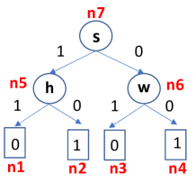
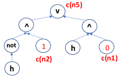
Figure 2: A decision tree and part of its compilation into an dDBC

5 Looking Ahead: Domain Knowledge

There are different approaches and methodologies to provide explanations in data management and artificial intelligence, with causality, counterfactuals and scores being prominent approaches that have a relevant role to play.

Much research is still needed on the use of contextual, semantic and domain knowledge in explainable data management and explainable machine learning, in particular, when it comes to define and compute attribution scores. Some approaches may be more appropriate in this direction, and we have argued that declarative, logic-based specifications can be successfully exploited [11]. For a particular application, maybe only some counterfactuals make sense, are reasonable or are useful; the latter becoming actionable or resources in that they may indicate feasible and achievable conditions (or courses of action) under which we could obtain a different result [46, 28].

Domain knowledge may come in different forms, among them:

1. In data management, via semantic constraints, in particular ICs, and ontologies that are fed by data sources or describe them. For example, satisfied ICs might make unnecessary (or prohibited) to consider certain counterfactual interventions on data. In this context, we might want to make sure that sub-instances associated to teams of tuples for Shapley computation satisfy a given set of ICs. Or, at the attribute level, that we do not violate constraints preventing certain attributes from taking null values.

2. In the context of machine learning, we could define an entity schema, basically a wide-predicate ${\it Ent}({\it Feat}_{1},\ldots,{\it Feat}_{n})$, on which certain constraints could be imposed. In our running example, we would have the entity schema ${\it Ent}(\mbox{\sf\small Name},\mbox{\sf\small Age},$ $\mbox{\sf\small Activity},\mbox{\sf\small Income},\mbox{\sf\small Debt},\mbox{\sf\small EdLevel})$; and depending on the application domain, local constraints, i.e. at the single entity level, such as:  (a) $\neg(\mbox{\sf\small Age}<\mbox{\sf\small 6}\wedge\mbox{\sf\small EdLevel}=\mbox{\sf\small phd})$, a denial constraint prohibiting that someone who is less than $6$ years old has a PhD;  (b) Or an implication  $\mbox{\sf\small Activity}=\mbox{\sf\small none}\rightarrow\mbox{\sf\small Income}=\mbox{\sf\small 0}$; etc.  Counterfactual interventions should be restricted by these constraints [11, sec. 6], or, if satisfied, they could be used to speed up a score computation. In [11, sec. 7], we showed how the underlying probability distribution, needed for Resp or Shap, can be conditioned by logical constraints of this kind.

   We could also have global constraints, e.g. requiring that any two entities whose values coincide for certain features must have their values for other features coinciding as well. This would be like a functional dependency in databases. This may have an impact of the subteams that are considered for Shap, for example.

3. Domain knowledge could also come in the form of probabilistic or statistical constraints, e.g. about the stochastic independence of certain features, or an explicit stochastic dependency of others via conditional distributions. In this direction, we could have a whole Bayesian network representing (in)dependencies among features. We could also have constraints indicating that certain probabilities are bounded above by a given number; etc. This kind of knowledge would have impact on attribution scores that are defined and computed on the basis of a given probability distribution.

The challenge becomes that of bringing these different forms of domain knowledge (and others) into the definitions or the computations of attribution scores.

Acknowledgments:  Part of this work was funded by ANID - Millennium Science Initiative Program - Code ICN17002; and NSERC-DG 2023-04650.

References

- [1]
- [2] Arora, S. and Barak, B. Computational Complexity. Cambridge University Press, 2009.
- [3] Arenas, M., Bertossi, L. and Chomicki, J. Consistent Query Answers in Inconsistent Databases. In Proc. ACM PODS 1999, pp. 68-79.
- [4] Arenas, M., Barcelo, P., Bertossi, L. and Monet, M. The Tractability of SHAP-scores over Deterministic and Decomposable Boolean Circuits. Proc. AAAI, 2021.
- [5] Arenas, M., Barcelo, P., Bertossi, L. and Monet, M. On the Complexity of SHAP-Score-Based Explanations: Tractability via Knowledge Compilation and Non-Approximability Results. Journal of Machine Learning Research, 2023, 24(63):1-58.
- [6] Bertossi. L. Database Repairing and Consistent Query Answering. Synthesis Lectures in Data Management. Morgan & Claypool, 2011.
- [7] Bertossi, L. and Salimi, B. From Causes for Database Queries to Repairs and Model-Based Diagnosis and Back. Theory of Computing Systems, 2017, 61(1):191-232.
- [8] Bertossi, L. Repair-Based Degrees of Database Inconsistency. Proc. LPNMR 2019, Springer LNCS 11481, pp. 195-209.
- [9] Bertossi, L. Specifying and Computing Causes for Query Answers in Databases via Database Repairs and Repair Programs. Knowledge and Information Systems, 2021, 63(1):199-231.
- [10] Bertossi, L., Li, J., Schleich, M., Suciu, D. and Vagena, Z. Causality-Based Explanation of Classification Outcomes. In Proceedings of the Fourth Workshop on Data Management for End-To-End Machine Learning, DEEM@SIGMOD 2020, pages 6:1-6:10, 2020.
- [11] Bertossi, L. Declarative Approaches to Counterfactual Explanations for Classification. Theory and Practice of Logic Programming, 23 (3): 559-593, 2023. arXiv Paper 2011.07423.
- [12] Bertossi, L. Attribution-Scores and Causal Counterfactuals as Explanations in Artificial Intelligence. In Reasoning Web: Causality, Explanations and Declarative Knowledge. Springer LNCS 13759, 2023.
- [13] Bertossi L. and Leon, J. E. Compiling Neural Network Classifiers into Boolean Circuits for Efficient Shap-Score Computation. Proc. AMW 2023, CEUR-WS Proc. Vol. 3409.
- [14] Bertossi L. and Leon, J. E. Efficient Computation of Shap Explanation Scores for Neural Network Classifiers via Knowledge Compilation. arXiv 2303.06516, 2023.
- [15] Bertossi, L., Kimelfeld, B., Livshits, E. and Monet, M. The Shapley Value in Database Management. ACM Sigmod Record, 2023, 52(2):6-17.
- [16] Bertossi, L. From Database Repairs to Causality in Databases and Beyond. To appear in special issue of Springer TLDKS dedicated to ‘Bases des Donnees Avances’ (BDA’22). arXiv 2306.09374, 2023.
- [17] Bryant, R. E. Graph-Based Algorithms for Boolean Function Manipulation. IEEE Tran. Com., C-35:677–691, 1986.
- [18] Chen, C., Lin, K., Rudin, C., Shaposhnik, Y., Wang, S. and Wang, T. An Interpretable Model with Globally Consistent Explanations for Credit Risk. arXiv 1811.12615, 2018.
- [19] Chockler, H. and Halpern, J. Responsibility and Blame: A Structural-Model Approach. J. Artif. Intell. Res., 2004, 22:93-115.
- [20] Darwiche, A. and Marquis, P. A Knowledge Compilation Map. Journal of Artificial Intelligence Research, 2002, 17:229–264.
- [21] Darwiche, A. On the Tractable Counting of Theory Models and its Application to Truth Maintenance and Belief Revision. Journal of Applied Non-Classical Logics, 2011, 11(1-2):11-34.
- [22] Flum, J. and Grohe, M. Parameterized Complexity Theory. Texts in Theoretical Computer Science, Springer, 2006.
- [23] Grant, J. and Martinez, M. V. (eds.) Measuring Inconsistency in Information. Studies in Logic 73, College Publications, 2018.
- [24] Halpern, J. and Pearl, J. Causes and Explanations: A Structural-Model Approach. Part I: Causes. The British journal for the philosophy of science, 2005, 56(4):843-887.
- [25] Halpern, J. Y. A Modification of the Halpern-Pearl Definition of Causality. In Proc. IJCAI 2015, pp. 3022-3033.
- [26] Holland, P.W. Statistics and Causal Inference. Journal of the American Statistical Association, 1986, 81(396):945-960.
- [27] Hunter, A. and Konieczny, S. On the Measure of Conflicts: Shapley Inconsistency Values. Artif. Intell., 174(14):1007–1026, 2010.
- [28] Karimi, A-H., Barthe, G., Schölkopf, B. and Valera, I. A Survey of Algorithmic Recourse: Contrastive Explanations and Consequential Recommendations. ACM Comput. Surv., 2023, 55(5):95:1-95:29.
- [29] Kivinen, J. and Mannila, H. Approximate Inference of Functional Dependencies from Relations. Theoretical Computer Science, 1995, 149:129-l49.
- [30] Livshits, E., Bertossi, L., Kimelfeld, B. and Sebag, M. The Shapley Value of Tuples in Query Answering. Logical Methods in Computer Science, 2021, 17(3):22.1-22.33.
- [31] Livshits, E., Bertossi, L., Kimelfeld, B. and Sebag, M. Query Games in Databases. ACM Sigmod Record, 2021, 50(1):78-85.
- [32] Livshits, E. and Kimelfeld, B. The Shapley Value of Inconsistency Measures for Functional Dependencies. Proc. ICDT 2021, pp. 15:1-15:19.
- [33] Lopatenko, A. and Bertossi, L. Complexity of Consistent Query Answering in Databases under Cardinality-Based and Incremental Repair Semantics. Proc. ICDT 2007, Springer LNCS 4353, pp. 179-193. Extended version with proofs: Arxiv cs.DB/1605.07159, 2016.
- [34] Lundberg, S. and Lee, S. A Unified Approach to Interpreting Model Predictions. In Proc. Advances in Neural Information Processing Systems, 2017, pp. 4765-4774.
- [35] Lundberg, S., Erion, G., Chen, H., DeGrave, A., Prutkin, J., Nair, B., Katz, R., Himmelfarb, J., Bansal, N. and Lee, S.-I. From Local Explanations to Global Understanding with Explainable AI for Trees. Nature Machine Intelligence, 2020, 2(1):2522-5839.
- [36] Meliou, A., Gatterbauer, W., Moore, K. F. and Suciu, D. The Complexity of Causality and Responsibility for Query Answers and Non-Answers. Proc. VLDB 2010, pp. 34-41.
- [37] Meliou, A., Gatterbauer, W., Halpern, J.Y., Koch, C., Moore, K. F. and Suciu, D. Causality in Databases. IEEE Data Engineering Bulletin, 2010, 33(3):59-67.
- [38] Papadimitriou, Ch. Computational Complexity. Addison-Wesley, 1994.
- [39] Pearl, J. Causality: Models, Reasoning and Inference. Cambridge University Press, 2nd edition, 2009.
- [40] Roth, A. E. (ed.) The Shapley Value: Essays in Honor of Lloyd S. Shapley. Cambridge University Press, 1988.
- [41] Rubin, D. B. Estimating Causal Effects of Treatments in Randomized and Nonrandomized Studies. Journal of Educational Psychology, 1974, 66:688-701.
- [42] Salimi, B., Bertossi, L., Suciu, D. and Van den Broeck, G. Quantifying Causal Effects on Query Answering in Databases. Proc. 8th USENIX Workshop on the Theory and Practice of Provenance (TaPP), 2016.
- [43] Gomes, C. P., Sabharwal, A. and Selman, B. Model Counting. Handbook of Satisfiability. IOS Press, 2009, pp. 993-1014.
- [44] Shapley, L. S. A Value for n-Person Games. Contributions to the Theory of Games, 1953, 2(28):307-317.
- [45] Shi, W., Shih, A., Darwiche, A. and Choi, A. On Tractable Representations of Binary Neural Networks. Proc. KR, 2020, pp. 882-892.
- [46] Ustun, B., Spangher, A. and Liu, Y. Actionable Recourse in Linear Classification. Proc. FAT 2019, pp. 10-19.
- [47] Valiant, L G. The Complexity Of Enumeration And Reliability Problems. Siam J. Comput., 1979, 8(3):410-421.
- [48] Van den Broeck, G., Lykov, A., Schleich, M. and Suciu, D. On the Tractability of SHAP Explanations. J. Artif. Intell. Res., 2022, 74: 851-886.
- [49] Wijsen, J. Database Repairing using Updates. ACM Trans. Database Syst., 2005, 30(3):722-768.