Learning Complex Motion Plans using Neural ODEs with Safety and Stability Guarantees

Abstract

We propose a Dynamical System (DS) approach to learn complex, possibly periodic motion plans from kinesthetic demonstrations using Neural Ordinary Differential Equations (NODE). To ensure reactivity and robustness to disturbances, we propose a novel approach that selects a target point at each time step for the robot to follow, by combining tools from control theory and the target trajectory generated by the learned NODE. A correction term to the NODE model is computed online by solving a quadratic program that guarantees stability and safety using control Lyapunov functions and control barrier functions, respectively. Our approach outperforms baseline DS learning techniques on the LASA handwriting dataset and complex periodic trajectories. It is also validated on the Franka Emika robot arm to produce stable motions for wiping and stirring tasks that do not have a single attractor, while being robust to perturbations and safe around humans and obstacles.

1 Introduction

Learning from Demonstrations (LfD) is a framework that enables transfer of skills to robots from observations of desired tasks (Khansari-Zadeh and Billard, 2011; Ijspeert et al., 2013; Yang et al., 2022). Typically, the observations are robot trajectories that are demonstrated through kinesthetic teaching, passively guiding the robot through the nominal motion to avoid the correspondence problem (Akgun and Subramanian, 2011). In such a framework, it is essential to learn motion plans from as few demonstrations as possible, while still providing required robustness, safety, and reactivity in a dynamic environment. While there are multiple approaches to represent the motion, we focus on Dynamical Systems (DS) based formulation (Billard et al., 2022a). DS based approaches have been shown to be particularly useful in Human-Robot Interaction (HRI) scenarios (Khansari-Zadeh and Billard, 2011; Figueroa and Billard, 2022; Khansari-Zadeh and Billard, 2014), where the robot inherently adapts to changes in the environment and can be compliant to human interactions, instead of following a stiff time-dependent reference motion that encodes the task.

Problem Formulation: A DS based motion plan for a robotic manipulator is defined in terms of the robot state variable $x\in\mathbb{R}^{d}$, where $x$ could be the robot’s end-effector Cartesian state or joint state. The motion planning layer is formulated as an autonomous DS

$$\dot{x}=f(x),$$ (1)

where $f(\cdot):\mathbb{R}^{d}\to\mathbb{R}^{d}$ is a nonlinear continuous function. The training data is $D$ demonstrations from kinesthetic teaching: $\mathcal{D}:=\{x_{i}(t_{1}),x_{i}(t_{2}),\ldots,x_{i}(t_{T})\}_{i=1}^{D}$, where, $x_{i}(t_{k})$ is the state of the robot at time $t_{k}$, for the $i^{th}$ demonstration. The discrete points in each demonstration are sampled uniformly at time $\{t_{1},t_{2},\ldots,t_{T}\}$. We assume that the training data trajectories $\mathcal{D}$ approximate an unknown nominal target trajectory $z^{*}(t)$ that encodes the task of the robot such as wiping, stirring, scooping, etc. Our aim is to design a vector field $f(\cdot)$ using the demonstrations $\mathcal{D}$ such that $x(t)$ follows the target trajectory $z^{*}(t)$. Previous work (Khansari-Zadeh and Billard, 2011; Figueroa and Billard, 2018) in the DS-based motion planning framework has considered convergence only to a single target. In this paper, we consider convergence to a trajectory $z^{*}(t)$ that can represent more complex, e.g., highly-nonlinear and periodic, motions. Under nominal circumstances, i.e., in the absence of disturbances or obstacles, the target trajectory $z^{*}(t)$ should be viewed as the reference for the low level controller to track. However, during deployment, the robot might not always follow the target trajectory because of tracking errors, disturbances, obstacles, etc. For example, there might be unanticipated perturbations during task execution which is generally not present while teaching a task for the robot. Consider the scenario in Fig. 1(a), where the target trajectory encodes a wiping task and the vector field is a unconstrained DS model (20) learned from demonstrations $\mathcal{D}$. As shown in Fig. 1(a), if the robot is perturbed by a disturbance during deployment to a region where there is no training data, the learned model commands the robot to a spurious attractor. However, the desired behaviour is to continue tracking the target trajectory so that the robot wipes the desired space as shown in Fig. 1(b). Ensuring robustness to perturbations is critical for deploying robots in human-centric environments, as disturbances can arise due to obstacles unseen in demonstrations and intentional or adversarial disturbances caused by humans (Billard et al., 2022a; Wang et al., 2022). This leads to our formal problem statement.

Problem 1

Given a set of training data $\mathcal{D}:=\{x_{i}(t_{1}),x_{i}(t_{2}),\ldots,x_{i}(t_{T})\}_{i=1}^{D}$, design a vector field $f(\cdot)$ for the dynamical system (20), such that it generates safe and stable motion plans at deployment for scenarios possibly not seen in the demonstrations, while ensuring that the robot’s trajectory $x(t)$ converges to the target trajectory $z^{*}(t)$.

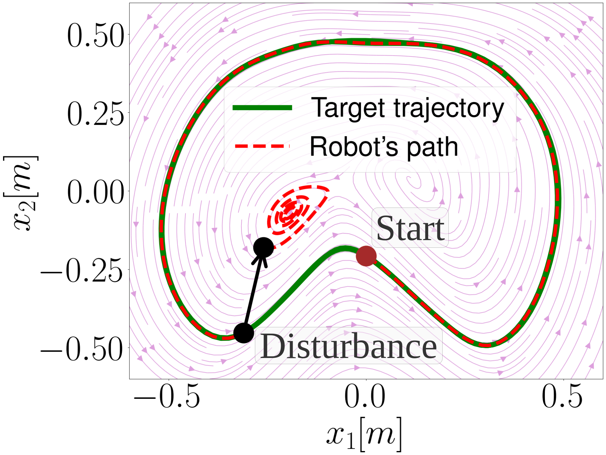
(a) Using standard NODE.

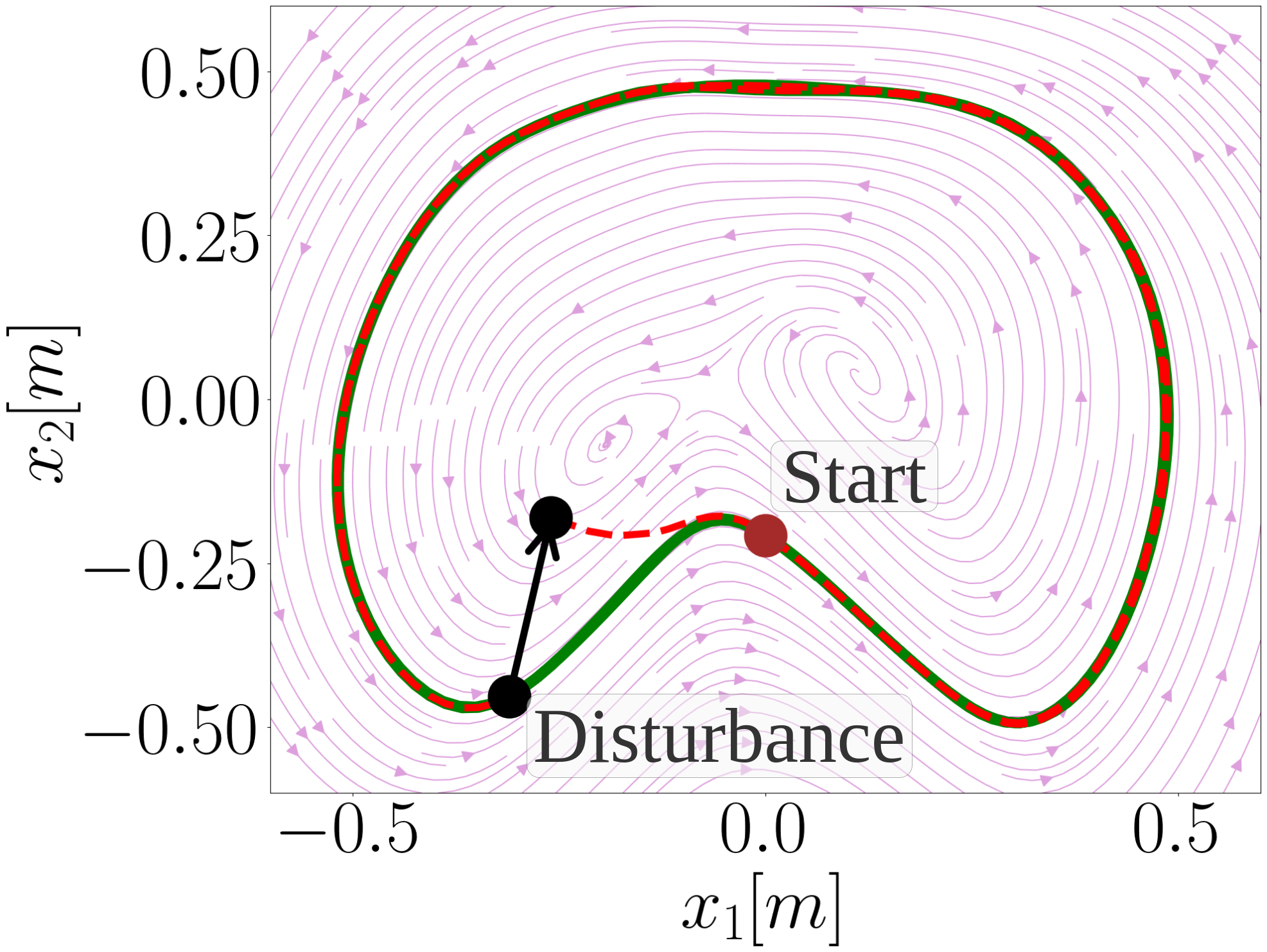
(b) Using CLF-NODE (ours)

Figure 1: An illustrative example of a spurious attractor when the robot’s path is guided by a DS-based motion plan in the presence of a disturbance is shown in (a) using NODE to encode the motion plan and (b) using the corrected CLF-NODE approach proposed in this work.

Related work: LfD is a widely used framework to learn the underlying motion policy of a task (Argall et al., 2009). Inverse Reinforcement Learning (IRL) and Behavior Cloning (BC) are popular methodologies that have been used to imitate motion from human demonstrations (Abbeel and Ng, 2004; Priess et al., 2014; Osa et al., 2018). In IRL, the underlying objective function of a task is learned and an optimization problem is solved to generate the robot motion. BC learns the state-action distribution of the task dynamics from demonstrations. IRL and BC typically require the demonstrator to explore the task space for learning the policy. Algorithms such as DAGGER (Ross et al., 2011) rely on online data collection for exploration. Exploration of the state space using large amounts of data may not be feasible for HRI applications, especially when the demonstrator is a human. We base our approach on DS-based LfD that has been shown to model stable motion plans from very few demonstrations (Khansari-Zadeh and Billard, 2011; Figueroa and Billard, 2022). One of the earliest work in DS-based LfD is called Dynamic Movement Primitives (Schaal, 2006) which estimates a nonlinear autonomous DS for various robotic applications such as walking, pouring, and grasping (Nakanishi et al., 2004; Ude et al., 2010). Stable Estimator of Dynamical Systems (SEDS) (Khansari-Zadeh and Billard, 2011) is a LfD method that learns globally stable dynamical systems with respect to a goal point using Gaussian Mixture Models (GMMs) and quadratic Lyapunov functions. An important limitation of SEDS is that it can only model trajectories whose distance to the target decrease monotonically in time. A method based on SEDS is presented in (Figueroa and Billard, 2018) via a Linear Parameter Varying (LPV) re-formulation of the model that learns more complex trajectories than SEDS. In (Ravichandar et al., 2017), contraction analysis is used to derive stability conditions on the learned trajectories. Recurrent Neural Networks (RNNs) have been used to model discrete motions (Reinhart and Steil, 2011; Lukoševičius and Jaeger, 2009). In (Chen et al., 2020), a Neural Network (NN) is used to learn the vector field $f(\cdot)$ in (20) and Lyapunov stability is imposed by a sampling algorithm that identifies unstable regions in a predefined workspace. In this work, we leverage the rich model class of NNs to capture the invariant features of the target trajectory, but use Neural Ordinary Differential Equations (Chen et al., 2019) instead of the standard regression model (Chen et al., 2020).

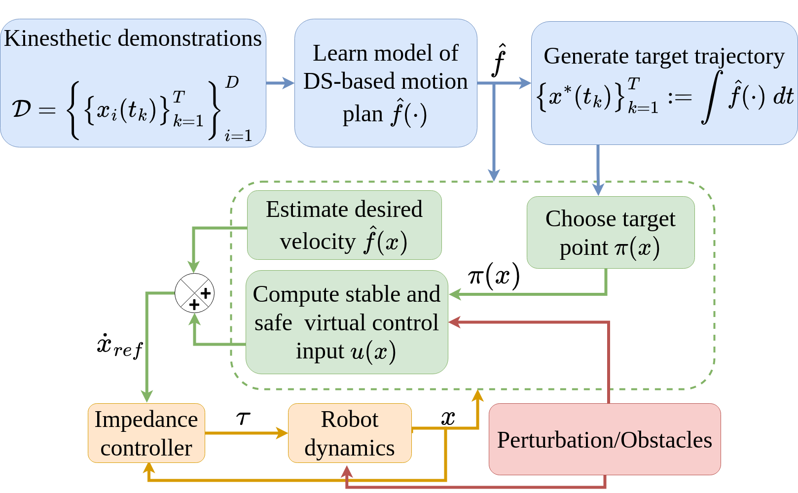
Figure 2: The modular control flow of our proposed pipeline using the CLF-CBF NODE approach. The state of the robot is $x$, the low level control input are the joint torques $\tau$, and the desired velocity in state space is $\dot{x}_{ref}$.

1.1 Proposed Approach

We parameterize the vector field (20) of the motion plan as

$$\dot{x}=\hat{f}(x)+u(x),$$ (2)

where, $\hat{f}(x)$ is used to encode the nominal system behavior, and $u(x)$ is used to enforce safety and disturbance rejection properties. We learn the nominal system $\hat{f}(\cdot)$ from demonstrations $\mathcal{D}$, and compute a correction term $u(x)$ based on control theoretic tools so that the goals of stability and safety are met in a composable, modular, and data efficient way. Similar to our objectives, the method proposed in (Figueroa and Billard, 2022) generates motion plans that not only converge to a global goal, but also has local stiff behaviours in regions around the target trajectory. Yet, they still lack in representing complex motions with high curvature and partial divergence. We use a modular approach similar to (Khansari-Zadeh and Billard, 2014), but, we define a CLF with respect to a time-varying target trajectory rather than a single goal point as assumed in (Khansari-Zadeh and Billard, 2014). Several DS-based obstacle avoidance methods (Hoffmann et al., 2009; Khansari-Zadeh and Billard, 2012) have been proposed that modulate the nominal dynamics of the motion by introducing a factor in the motion equation. Control Barrier Functions (CBFs) (Robey et al., 2020; Ames et al., 2019) are widely used to enforce safety of dynamical systems, and we adopt them in this work to generate safe motion plans.

A schematic of the proposed control flow is presented in Fig. 2. The blue blocks represent the offline learning component and the green blocks are the online computation modules. We use a neural network parameterized model $\hat{f}$ that we learn from demonstrations $\mathcal{D}$, but any other model class could be used within our proposed framework. Starting from an initial condition, we integrate $\hat{f}(\cdot)$ for the same time span of the task given in demonstrations to generate a target trajectory $x^{*}(t)$ that approximates the unknown nominal target trajectory $z^{*}(t)$. At deployment, the actual states of the robot $x$ are observed by our motion plan at every time $t$. Given the current state $x$, our architecture then chooses the target point $\pi(x)$ that the robot should follow at time $t$ using the pre-computed target trajectory $x^{*}(t)$. We estimate the nominal desired velocity $\hat{f}(x)$ using our learnt model. However, as illustrated in Fig. 8, the generated motion plan from $\hat{f}$ is neither guaranteed to be stable nor safe. Hence, we compute a virtual control input $u(x)$ as an additive correction term that generates the reference motion plan $\dot{x}$ using (2) so that the trajectory generated by $\dot{x}$ converges to the target trajectory even in the presence of disturbances and unsafe regions such as obstacles. We denote the reference velocity for the low level controller as $\dot{x}_{ref}$, which in general may be different from the real velocity $\dot{x}$ of the robot. The reference velocity $\dot{x}_{ref}$ is given as input to the impedance controller (Kronander and Billard, 2016a) that computes the low level control input $\tau$ (joint torques) for the physical robotic system. We emphasize that the virtual control input $u(x)$ is different from the low-level control inputs $\tau$ given in Fig. 2, and is a component of the motion planning DS (2).

Contributions Our contributions are given below.

1. We propose a Neural ODE (NODE) based offline learning methodology that captures the invariant features of complex nonlinear and periodic nominal motion plans, such as wiping and stirring, using only a few demonstrations from kinesthetic teaching.

2. We generate a DS-based reactive motion policy for HRI scenarios by solving an efficient Quadratic Program (QP) online at high frequency that integrates CLFs and CBFs as constraints on the nominal NODE-based motion plan to guarantee stability and safety, respectively.

3. We define a novel look-ahead strategy that chooses a target point at every time step for the robot to follow, enabling tracking of a time-varying target trajectory instead of a single target point.

4. We show significant performance improvements over existing methods on the LASA handwriting data set, and validate that our approach enables complex nonlinear and periodic motions for compliant robot manipulation on the Franka Emika robot arm.

2 Learning Nominal Motion Plans using Neural ODEs

We propose a neural network parameterized function class to learn the dynamics of the motion offline from demonstrations. Although existing work (Figueroa and Billard, 2022) has provided guarantees on stable learning of dynamical systems using mixture of linear models that converge to a single target, we aim to learn more complex trajectories that also generalize across the task space and scale to higher dimensions. Since neural networks have demonstrated high capability for accurate time-series modeling (Chen et al., 2020), we base our approach on Neural ODEs (Chen et al., 2019), which are the continuous limit (in depth) of ResNets (Haber and Ruthotto, 2017). We parameterize our models of nominal target trajectories as:

$$\frac{d\hat{x}(t)}{dt}=f_{\theta}(\hat{x}(t)),$$ (3)

where $f_{\theta}(\cdot):\mathbb{R}^{d}\to\mathbb{R}^{d}$ is a neural network with parameters $\theta$, and $\hat{x}(t)\in\mathbb{R}^{d}$ is the state variable predicted by $f_{\theta}(\cdot)$ at time $t$. In the forward pass, given the integration time interval $[a,b]$ and an initial point $\hat{x}(a)$, the model outputs the trajectory $\hat{x}(t)$ for $t\in[a,b]$. The trajectory is obtained by solving the differential equation in (19) using a general-purpose differential equation solver based on fifth-order Runge-Kutta (Butcher, 1996). We set $f_{\theta}(\cdot)$ to be a Multi-Layer Perceptron (MLP), where the inputs and outputs are in $\mathbb{R}^{d}$ so that the trajectory predictions evolve in the relevant state space.

We consider the supervised learning setup with training data $\mathcal{D}$. The predictions of the state $\hat{x}_{i}(t_{k})$ by the model $f_{\theta}$ are obtained via integration:

$$\hat{x}_{i}(t_{k+1}) =\hat{x}_{i}(t_{k})+\int_{t_{k}}^{t_{k+1}}f_{\theta}(\hat{x}_{i}(s))\ ds,\forall\ k\in\{1,2,\ldots,T-1\}$$ (4)

where we set $\hat{x}_{i}(t_{1})=x_{i}(t_{1}),\ \forall\ i\in\{1,2,\ldots,D\}$. We apply empirical risk minimization with loss

$$\min_{\theta}\frac{1}{DT}\sum_{i=1}^{D}\sum_{k=1}^{T}\Bigl{\|}x_{i}(t_{k})-\hat{x}_{i}(t_{k})\Bigr{\|}_{2}^{2},$$ (5)

to learn the parameters $\theta$, where the predictions $\hat{x}_{i}(t_{k})$ are generated as in (4). In contrast to previous work (Figueroa and Billard, 2022; Khansari-Zadeh and Billard, 2014) which learns a map $\hat{f}(x(t))$ using labeled data $\{x(t),\dot{x}(t)\}$, we do not assume access to velocity measurements as they are often not easily collected and/or noisy (Purwar et al., 2008; Xiao et al., 2020). Further, noisy velocity measurements might cause the map to overfit and lead to aggressive trajectories at inference that are not desirable for the low-level controller. From our results presented in Fig. 8 and Section 4, we observe that the NODE model generates smooth trajectories utilizing only state variables $x(t)$ to learn $f_{\theta}$ and not their derivatives $\dot{x}(t)$. While such a NODE-based vector field will behave reliably on and near the training data, if there are unanticipated disturbances or obstacles during deployment, the robot might deviate to regions of the state-space where the learned vector field is unreliable. Next, we present a methodology that computes a correction term to ensure that the robot robustly and safely tracks the learned target trajectory.

3 Enforcing Stability and Safety via Virtual Control Inputs

We begin with a review of control theoretic tools that provide sufficient conditions for stability and safety of dynamical systems. We consider a nonlinear control affine dynamical system

$$\dot{x}=g(x)+h(x)u,$$ (6)

where, $x\in\mathcal{X}\subset\mathbb{R}^{d}$ and $u\in\mathcal{U}\subset\mathbb{R}^{m}$ are the set of allowable states and control inputs, respectively. The DS-based motion plan (2) is a nonlinear control affine DS with $g(x)=\hat{f}(x)$ and $h(x)=1$.

3.1 Control Lyapunov Functions

We consider the objective of asymptotically stabilizing the DS (6). Without loss of generality, we focus on stabilizing the system to the origin: ${x^{*}=0}$. If we can find a control law $u$ that decreases a positive definite function $V(\cdot):\mathbb{R}^{d}\to\mathbb{R}_{\geq 0}$ to zero for the dynamics (6), then, asymptotic stability is guaranteed. Such a function $V(\cdot)$ is termed as a CLF and the formal definition is given below (Ames et al., 2019).

Definition 1

A continuously differentiable function $V(\cdot):\mathbb{R}^{d}\to\mathbb{R}_{\geq 0}$ is a Control Lyapunov Function (CLF) for the dynamical system (6) if it is positive definite and there exists a class $\mathcal{K}_{\infty}$ function $\alpha(\cdot):\mathbb{R}_{\geq 0}\to\mathbb{R}_{\geq 0}$ that satisfies

$$\inf_{u\in\mathcal{U}}\nabla_{x}V(x)^{\top}\left(g(x)+h(x)u\right)\leq-\alpha(V(x)),\ \forall\ x\in\mathcal{X}.$$ (7)

A function $\alpha(\cdot)$ belongs to class $\mathcal{K}_{\infty}$ if $\alpha(0)=0$ and $\alpha(\cdot)$ is strictly increasing. The set of all controllers that satisfy the condition in (7) for each $x\in\mathcal{X}$ is

$$K_{clf}(x):=\{u\in\mathcal{U}:\nabla_{x}V(x)^{\top}\left(g(x)+h(x)u\right)\leq-\alpha(V(x))\}.$$ (8)

The following result on asymptotic stability follows from (Ames et al., 2019).

Theorem 1

If there exists a Control Lyapunov Function (CLF) as given in Definition 7 for a nonlinear control affine system (6), then, any Lipschitz continuous feedback control law $u(x)\in K_{clf}(x)$ asymptotically stabilizes the dynamical system (6) to the origin ${x^{*}=0}$.

3.2 Control Barrier Functions

We define safety with respect to a safe set $\mathcal{C}\subseteq\mathcal{X}$ for the system (6). The safe set $\mathcal{C}$ is defined as the super-level set of a function $B(\cdot):\mathbb{R}^{d}\to\mathbb{R}$, that results in three important sets:

$$\mathcal{C}=\{x\in\mathcal{X}:B(x)\geq 0\},\ \mathcal{\partial C}=\{x\in\mathcal{X}:B(x)=0\},\ \textnormal{Int}(\mathcal{C})=\{x\in\mathcal{X}:B(x)>0\},$$ (9)

where $\mathcal{\partial C}$ is the boundary for safety and $\textnormal{Int}(\mathcal{C})$ is the interior of the safe set $\mathcal{C}$. Our safety objective is to find a control input $u$ such that the states $x$ that evolve according to the dynamics (6) always stay inside the safe set $\mathcal{C}$. Such an objective is formalized using forward invariance of the safe set $\mathcal{C}$. Let $u(x)$ be a feedback control law such that closed loop dynamical system

$$\dot{x}=g(x)+h(x)u(x)$$ (10)

is locally Lipschitz. The locally Lipschitz condition guarantees the existence of a unique solution $x(t)$ to (10) for a given initial condition $x_{0}=x(0)$ and all $t\in[0,t_{max})$. If $t_{max}=\infty$, then the system (10) is forward complete (Khalil, 2015). Forward invariance and CBFs are defined as follows (Ames et al., 2019).

Definition 2

The safe set $\mathcal{C}$ is forward invariant if for every initial point $x(0)=x_{0}\in\mathcal{C}$, the future states $x(t)\in\mathcal{C}$ for all $t\geq 0$.

Definition 3

Let $\mathcal{C}$ be the super-level set of a continuously differentiable function $B(\cdot):\mathbb{R}^{d}\to\mathbb{R}$ as given in (9). Then, $B$ is a Control Barrier Function (CBF) for the dynamical system (6) and safe set $\mathcal{C}$ if there exists an extended class $\mathcal{K}_{\infty}$ function $\gamma(\cdot)$ that satisfies

$$\sup_{u\in\mathcal{U}}\nabla_{x}B(x)^{\top}\left(g(x)+h(x)u\right)\geq-\gamma(B(x)),\ \forall\ x\in\mathcal{X}.$$ (11)

We aim to render the set $\mathcal{C}$ forward invariant for the system (10) through an appropriate choice of control input $u(x)$. The set of all control inputs that satisfy the condition in (11) for each $x\in\mathcal{X}$ is

$$K_{cbf}(x):=\{u\in\mathcal{U}:\nabla_{x}B(x)^{\top}\left(g(x)+h(x)u\right)\geq-\gamma(B(x))\}.$$ (12)

The formal result on safety follows from (Ames et al., 2019).

Theorem 2

Let $B$ be a Control Barrier Function (CBF) as given in Definition 11 for a safe set $\mathcal{C}$ and a nonlinear control affine system (6). Let $u(x)\in K_{cbf}(x)$ be a locally Lipschitz feedback control law. Then, the following holds: $x(0)\in\mathcal{C}\implies x(t)\in\mathcal{C}$ for all $t\in[0,t_{max})$. If the set $\mathcal{C}$ is compact, then, $\mathcal{C}$ is forward invariant, i.e., $t_{max}=\infty$, and $\mathcal{C}$ is asymptotically stable, i.e., $\lim_{t\to\infty}x(t)\in\mathcal{C}$ for all $x(0)\in\mathcal{X}$.

Since inequalities in (8) and (12) are affine in $u$, they can be included in efficient optimization-based controllers for control affine systems. We present such an optimization-based planner in Section 3.3 that has strong stability and safety guarantees as claimed in Theorems 1 and 2, respectively.

3.3 Computing the Virtual Control Input

We now show how to integrate CLFs and CBFs into the DS-based motion plan (2). In particular, we use the learned NODE $f_{\theta}$ to generate nominal motion plans, and compute $u(x)$ using CLFs and CBFs to enforce stability and safety, resulting in a DS-based motion plan of the form:

$$\dot{x}=f_{\theta}(x)+u(x),$$ (13)

where $x$ is the state of the robot, and $u(x)$ is the virtual control input.

Stability using Control Lyapunov Functions

We utilize CLFs described in Section 3.1 to generate a motion plan that always converge to the target trajectory $x^{*}(t)$ even in the presence of disturbances. Previous work (Khansari-Zadeh and Billard, 2014) have utilized CLFs only for convergence to a single target point using regression methods. In contrast, we present a framework that integrates Neural ODEs for rich behaviors, CBFs for safety, and CLFs to ensure convergence to a target trajectory $x^{*}(t)$. To that end, we first define the error $e(t)$ between the robot state and the target trajectory: $e(t)=x(t)-x^{*}(t)$. For ease of notation, we drop the explicit dependence on time $t$, and write $e$, $x$, and $x^{*}$ for the current error, state, and target point at time $t$, respectively. From (13), the error dynamics are given by

$$\dot{e}=\dot{x}-\dot{x}^{*}\Rightarrow\dot{e}=f_{\theta}(x)-\dot{x}^{*}+u(x)$$ (14)

The error dynamics (14) define a nonlinear control affine system  (6), where the state of the system is $e$, and $u(x)$ is the control input. Hence, by Theorem 1, if there exists a CLF $V(\cdot)$ for the error dynamics (14), then, any feedback virtual control law $u(\cdot)$ that satisfies

$$\nabla_{e(t)}V(e)^{\top}\left(f_{\theta}(x)-\dot{x}^{*}+u(x)\right)\leq-\alpha(V(e)),\ \forall\ e\in\mathbb{R}^{d}$$ (15)

will drive the error asymptotically to zero. During online motion planning, given the current state of the robot $x$ and information about the target trajectory $x^{*}$ that encodes the desired task, we compute the smallest $u(x)$ that satisfies (15) by setting

$$u(x)=\operatorname*{argmin}_{v}\bigl{\|}v\bigr{\|}^{2}_{2}\quad\textnormal{s.t.} \nabla_{e}V(e)^{\top}\left(f_{\theta}(x)-\dot{x}^{*}+v\right)\leq-\alpha(V(e)),$$ (16)

where $\alpha(\cdot)$ is a class $\mathcal{K}_{\infty}$ function that defines how aggressively the robot tracks the target trajectory. We described how we choose $x^{*}$ and $\dot{x}^{*}$ in detail in Section 3.3. The optimization problem (22) is a Quadratic Program (QP) with a single affine inequality and has a closed form solution (Khansari-Zadeh and Billard, 2014). The Lyapunov function we use is $V(e)=\|e\|_{2}^{2}$, but, note that any positive definite function is a valid CLF due to the presence of the virtual actuation term $v$, i.e., optimization problem (22) is always feasible. We refer the reader to Fig. 8 to differentiate between the paths generated by only $f_{\theta}(\cdot)$, and by (13) using the correction term $u(\cdot)$. We refer to this approach as the CLF-NODE.

Safety using Control Barrier Functions

We build on the framework presented in Section 3.2 by integrating CBFs into the virtual control input computation to guarantee safety for the generated motion plan. We define safety with respect to a safe set $\mathcal{C}\subseteq\mathcal{X}$ as described in Section 3.2 for the system (13). From Theorem 2, if there exists a CBF $B(\cdot)$ for the dynamics (13), then, any feedback control law $u(\cdot)$ that satisfies

$$\nabla_{x}B(x)^{\top}\left(f_{\theta}(x)+u(x)\right)\geq-\gamma(B(x)),\ \forall\ x\in\mathcal{X}$$ (17)

will render the system (13) safe, where, $\gamma(\cdot)$ is an extended class $\mathcal{K}_{\infty}$ function. At inference, the DS-based motion plan is still given by (13), but the virtual control input $u(x)$ is computed such that it satisfies the CBF condition in (17) for the dynamics $\dot{x}$ and a given CBF $B(\cdot)$ for the safe set $\mathcal{C}$.

In cases where an obstacle obstructs the robot moving along the nominal trajectory, the robot should automatically avoid the obstacle without human intervention, but converge back to complete the desired task when possible. However, this may lead to a conflict between preserving safety and stability: during the obstacle avoidance phase, the CLF constraint in (22) may be violated as the robot takes safety preserving actions that increase tracking error. We prioritize safety and obstacle avoidance and adapt the approach proposed in (Ames et al., 2019) for balancing these competing objectives to our setting, and solve an optimization problem with the CBF condition (17) as a hard constraint and the CLF condition (15) as a soft constraint. Given the current state of the robot $x$ and the target point $x^{*}$, the optimization problem that guarantees a safe motion plan is

$$(u(x),\_)=\operatorname*{argmin}_{\{v,\epsilon\}}\quad\bigl{\|}v\bigr{\|}^{2}_{2}+\lambda\epsilon^{2}\quad\textnormal{s.t.} \nabla_{x}B(x)^{\top}\left(f_{\theta}(x)+v\right)\geq-\gamma(B(x))$$ (18)

$$\nabla_{e}V(e)^{\top}\left(f_{\theta}(x)-\dot{x}^{*}+v\right)\leq-\alpha(V(e))+\epsilon$$

where $\epsilon$ is a relaxation variable to ensure feasibility of (24) and is penalized by $\lambda>0$. The problem in (24) is a parametric program, where the parameters of interest are $\{x,x^{*},\dot{x}^{*}\}$. We abuse notation and denote the optimal virtual control input $u(x)$ for (24) to be $u(x,x^{*},\dot{x}^{*})$ which will be used in the next section. Problem (24) is a QP that can be solved efficiently in real-time (Mattingley and Boyd, 2012). Multiple CBFs and CLFs can be composed in a way analogous to problem (24) to represent multiple obstacles. We refer to this approach as the CLF-CBF-NODE.

Choosing a Target Point

Input: $\mathcal{T}:=\{x^{*}(t_{k})\}_{k=1}^{T},f_{\theta}(\cdot),x,N$

Output: $\pi(x)$

$m\leftarrow\operatorname*{argmin}_{k}\big{\|}x-x^{*}(t_{k})\big{\|}_{2}$;

${\mathcal{T}_{N}:=\{x^{*}(t_{m}),x^{*}(t_{m+1}),\ldots,x^{*}(t_{N})\}}$;

Solve (24) with parameters $\{x,y,f_{\theta}(y)\}$ for each $y\in\mathcal{T}_{N}$;

$\pi(x)\leftarrow\operatorname*{argmin}_{y\in\mathcal{T}_{N}}\big{\|}u(x,y,f_{\theta}(y))\big{\|}_{2}^{2}$;

Algorithm 1 Choose target point

As shown in Fig. 2, we first integrate the learnt model $f_{\theta}(\cdot)$ offline to generate the target array ${\mathcal{T}:=\{x^{*}(t_{k})\}_{k=1}^{T}}$ from a given initial condition $x^{*}(t_{1})$. Given an observation of the current state of the robot $x$ at time $t$, and the target array $\mathcal{T}$, we select the next target point $x^{*}$ for the robot to follow using the map $\pi(x)$ defined in Algorithm 2. We remove the direct dependence of the target point $x^{*}$ on time $t$, which leads to a more reactive motion plan that adapts to both the time delays that are often present during online deployment, and to unforeseen perturbations of the robot away from the nominal plan, e.g., due to human interaction or obstacle avoidance. The look-ahead horizon length $N$ is used to construct the look-ahead array $\mathcal{T}_{N}$, consisting of $N$ future points starting at the current state $x^{*}(t_{m})$. We choose the target point $\pi(x)$ from $\mathcal{T}_{N}$ that results in the smallest norm of virtual control input when solving (24) amidst all points in $\mathcal{T}_{N}$. We use a forward looking horizon $N$ to ensure the robot moves forward along the target trajectory, and to the best of our knowledge, this is the first time that the norm of the correction input $u(\cdot)$ is used as a metric for choosing an appropriate nearest neighbor point in motion planning. We use $\dot{x}^{*}:=f_{\theta}(\pi(x))$, since $\pi(x)\in\mathcal{T}$ and we obtained the target array $\mathcal{T}$ by integrating $f_{\theta}(\cdot)$.

4 Experimental Validation and Results

LASA handwriting dataset We validate our approach on the LASA 2D handwriting data set (Khansari-Zadeh and Billard, 2011) that contains 30 nonlinear motion sets. Each set has $7$ demonstrations: we use 4 as the training data set, and the remaining three as the test data set. The performance metric we use is Dynamic Time Warping (DTW) distance (Salvador and Chan, 2007) to compare our NODE model with two existing DS-based learning approaches: SEDS (Khansari-Zadeh and Billard, 2011) and LPV-DS (Figueroa and Billard, 2018). DTW distance measures the dissimilarity between the shapes of the demonstrations and the corresponding reproductions starting from the same initial condition. The DTW distance comparison is given in Figs. 3(a) and 3(b). We note that although SEDS and LPV-DS use velocity data for regression, which our approach does not have access to, the DTW distance for our NODE approach is approximately half that of existing methods (Khansari-Zadeh and Billard, 2011; Figueroa and Billard, 2018). We illustrate disturbance rejection in Fig. 4(a) using CLF-NODE and obstacle avoidance in Fig. 4(b) using CLF-CBF-NODE. Further validation on other nonlinear shapes are given in the appendix.

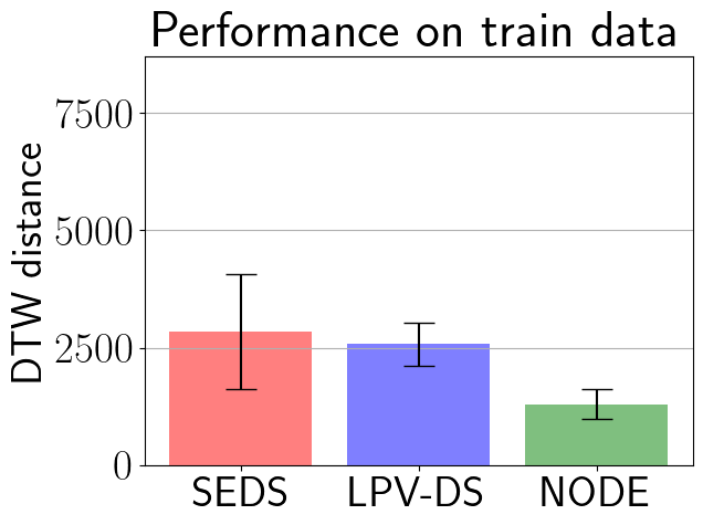
(a) Train data set

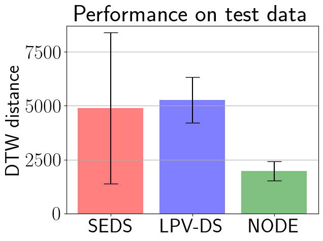
(b) Test data set

Figure 3: Comparison of DTW distance on the (a) Train data set and (b) Test data set from LASA.

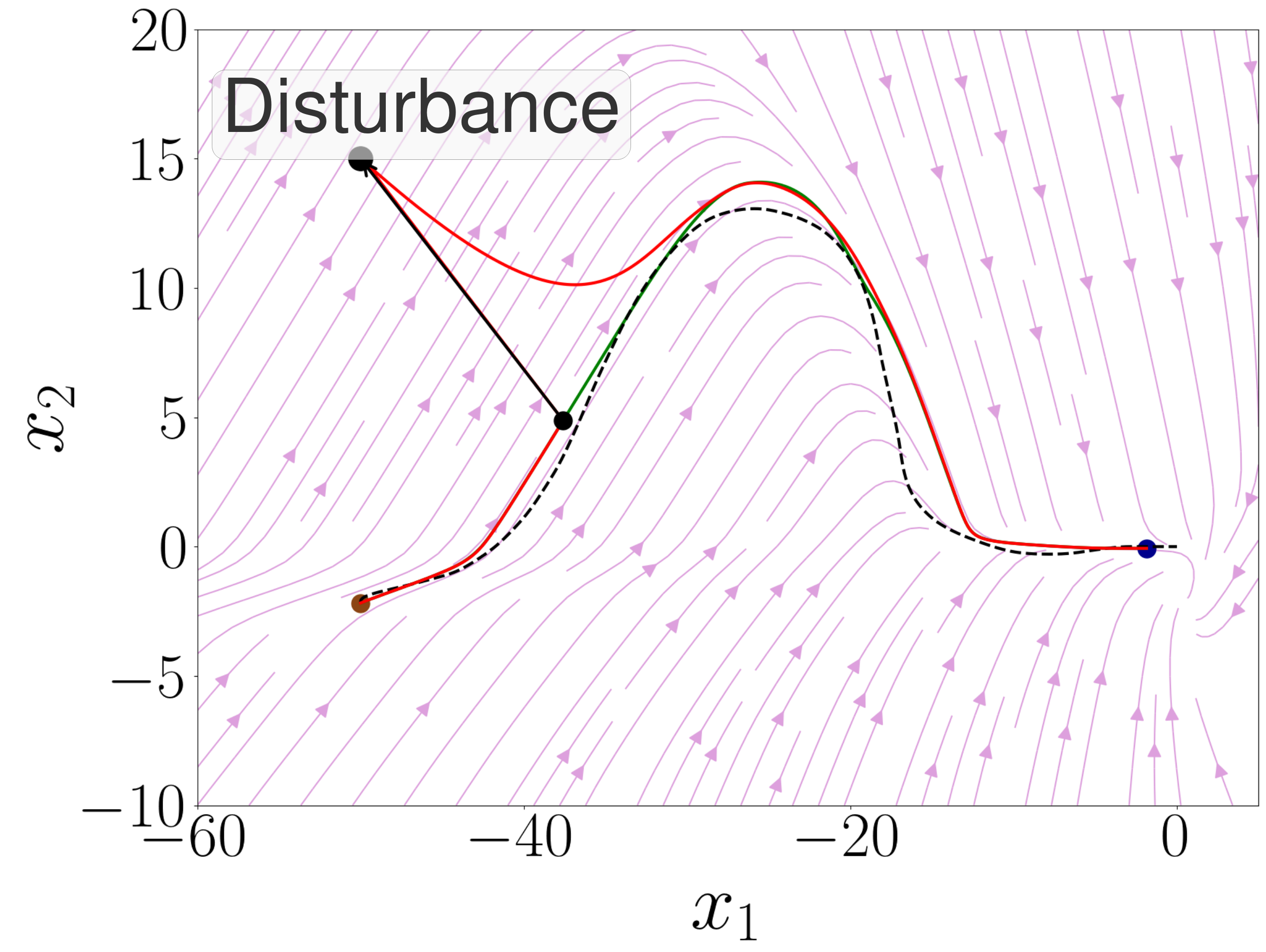
(a) Worm with disturbance.

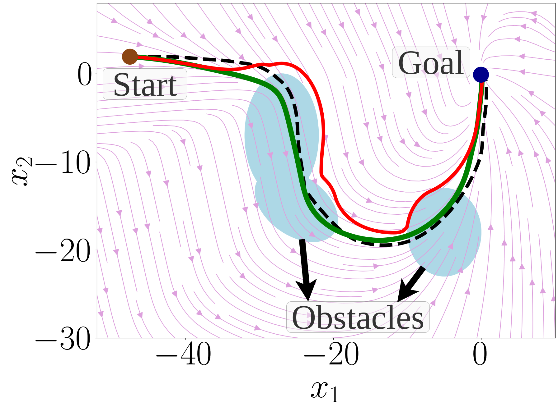
(b) Spoon with obstacles

Figure 4: Illustration of (a) disturbance rejection and (b) obstacle avoidance using our approach.

Periodic trajectories: We validate our approach on handwritten 2D periodic motions of the letters I, R, O and S given in (Urain et al., 2020) and 3D periodic trajectories that encode three wiping tasks as given in Figs. 5(e), 6, and 7. We compare our method with Imitation Flow (IFlow) (Urain et al., 2020) and a Gaussian Process (GP) (Jaquier et al., 2019) based approach. IFlow is based on normalizing flows that learns stable motions using prior knowledge on whether the underlying dynamics of the demonstrations has a single attractor or a limit cycle, but our approach requires no prior knowledge. We present the DTW distance in Fig. 5(a), training time in Fig. 5(b) and execution time in Fig. 5(c). The execution time is the computation time for a single forward pass of the model to generate the entire trajectory from a given initial point and the time span of the demonstration. We also compare the trajectory reproductions for the R shape in Fig. 5(d), and for the spiral wiping task by the Franka robot arm in Fig. 5(e). The IFlow approach is not able to learn the complex motion for spiral wiping, but our NODE approach learns with high accuracy and lesser computation time. The execution time comparison in Fig. 5(c) is plotted in $\log$ scale and we note that our approach (NODE) has much lesser execution time, which is important for real-time robot experiments. Although the GP based method (Jaquier et al., 2019) is able to learn complex trajectories with comparable accuracy and training time to NODE, the execution time is much smaller and they rely on time inputs for desired roll outs with no capability to generate safe and stable motion plans. All computations are performed on Google Colab.

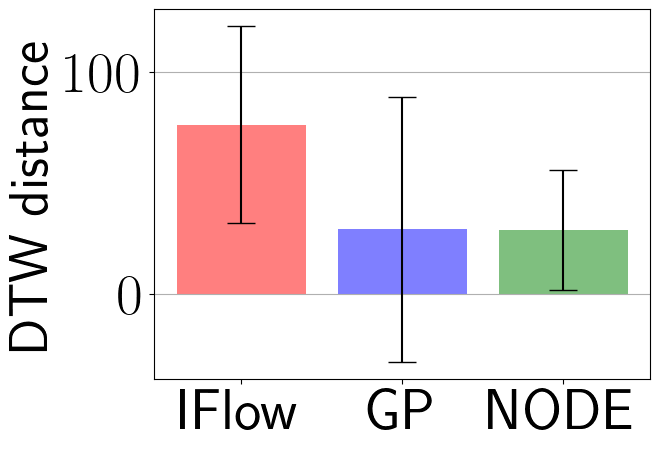
(a) DTW distance

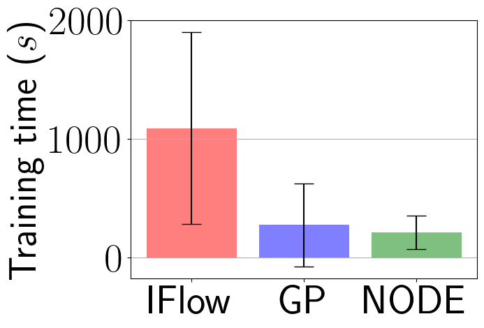
(b) Training time

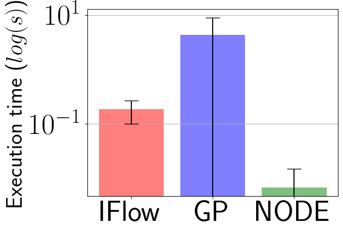
(c) Execution time

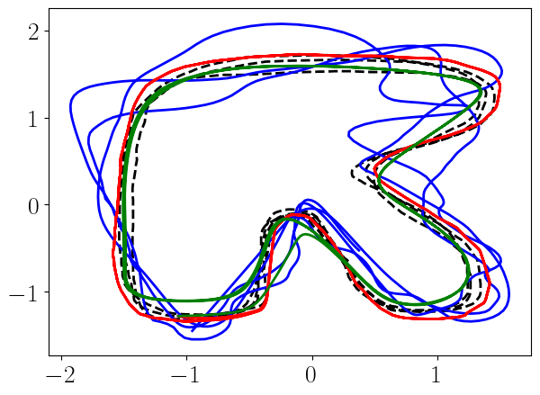
(d) R shape

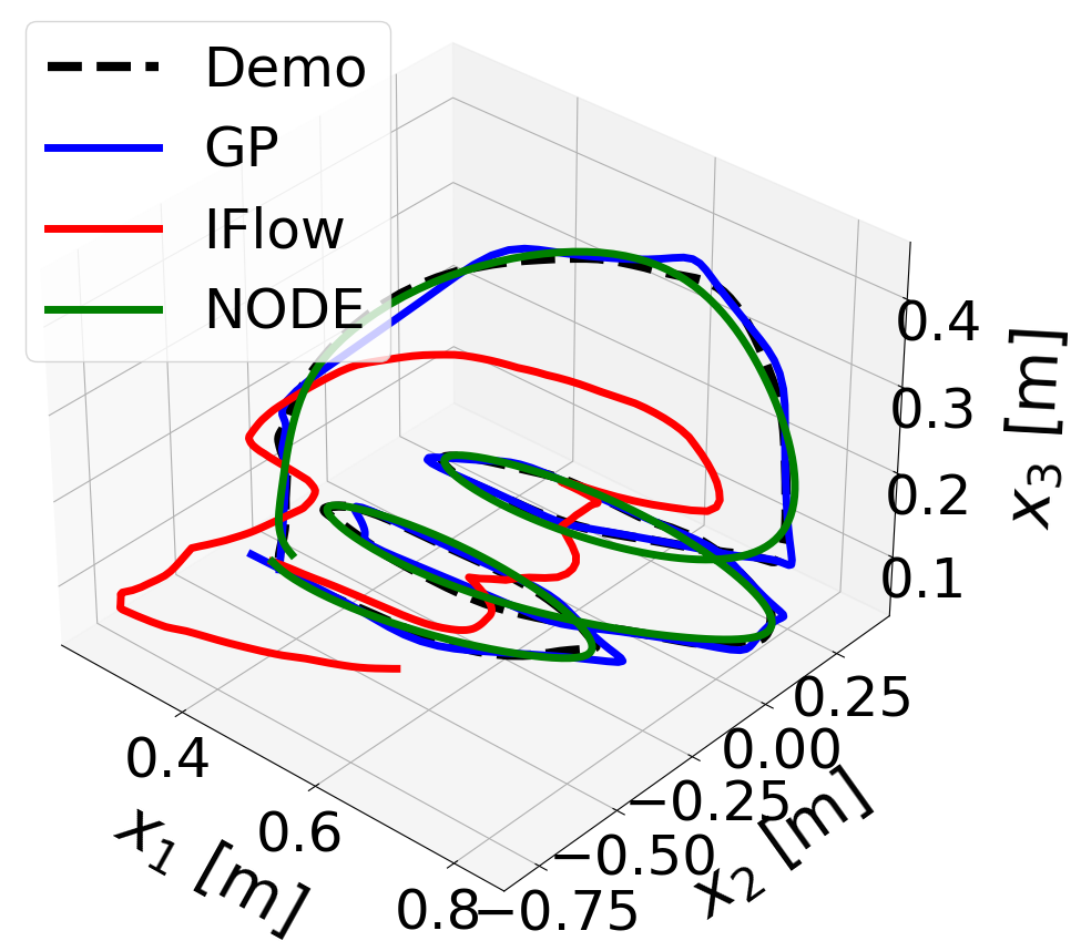
(e) Spiral wiping

Figure 5: Comparison of performance metrics and trajectory reproductions between IFlow, GP and our approach (NODE) on periodic trajectories.

Robotic experiments We validate our approach on the Franka Emika robot arm performing two complex nonlinear motions: wiping a human mannequin with a towel as shown in Fig. 6 and wiping a white board with an eraser as given in Fig. 7. We use the passive DS impedance controller given in (Kronander and Billard, 2016b). We used $D=2$ demonstrations for the mannequin tasks, and $D=3$ demonstrations for the board wiping tasks. Each demonstration had between $T=300$ and $T=600$ data samples. The average training time (offline) is $3-6$ minutes for each task on Google Colab. The obstacle shown in Fig. 7 at $t=2$ has markers on it that are tracked in real-time by OptiTrack motion capture system. We observe that the robot tracks the desired nominal trajectories while remaining compliant to human interaction, robust to perturbations, and safe with respect to unforeseen and dynamic obstacles. We include the stirring task and other implementation details in the appendix.

Further illustrations of disturbance rejection, obstacle avoidance and trajectory reproductions are presented in https://sites.google.com/view/lfd-node-clf-cbf/home.

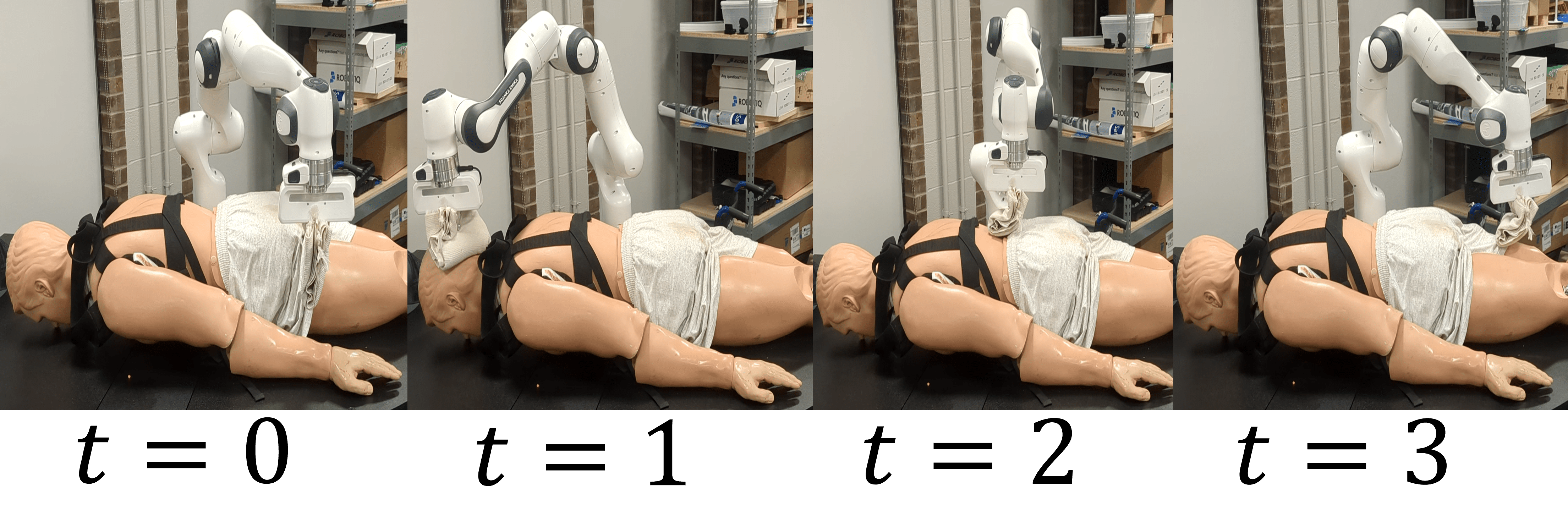
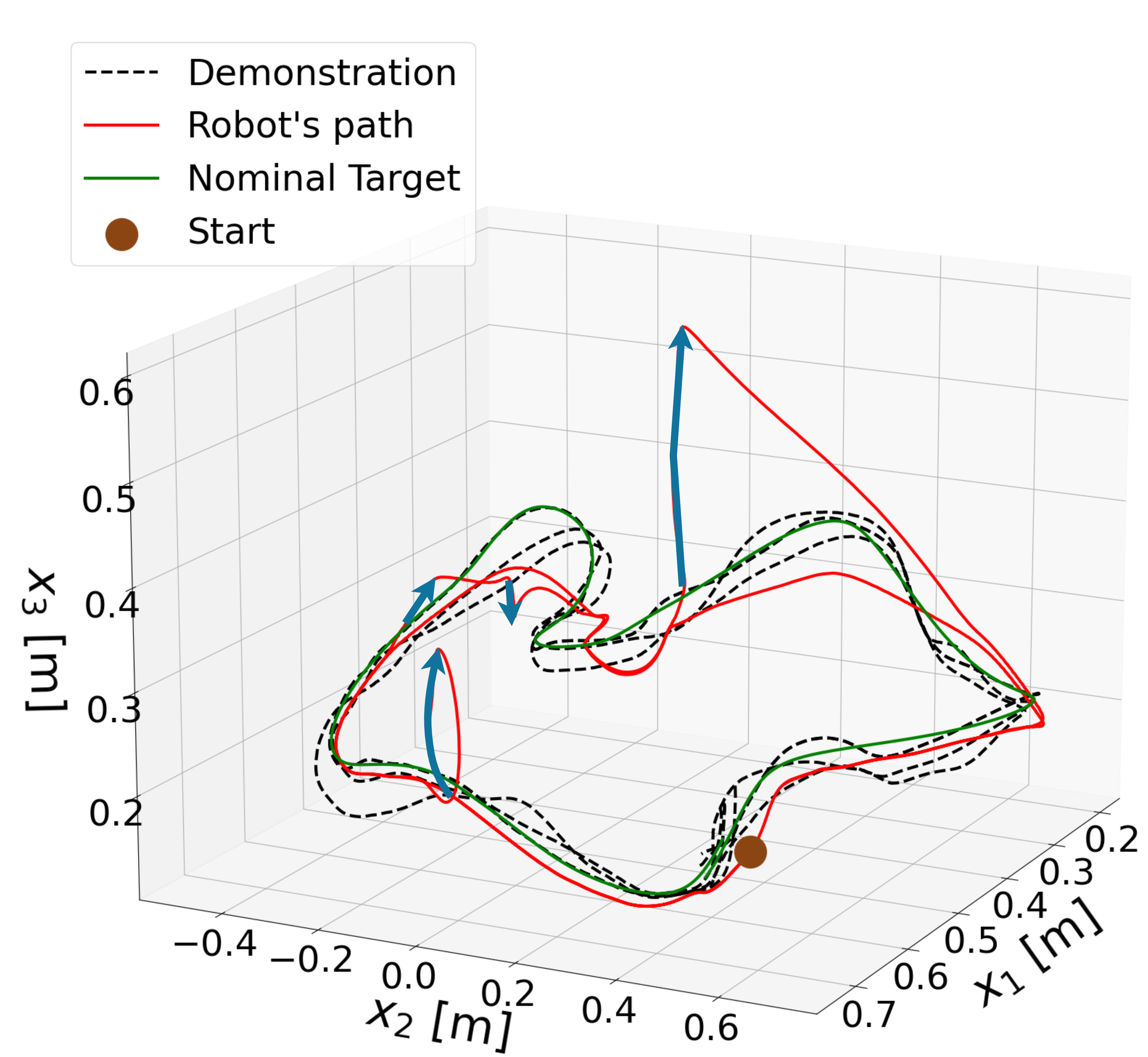
Figure 6: Franka Emika robot arm performing a periodic wiping task for a human mannequin. The blue arrows denote the perturbation.

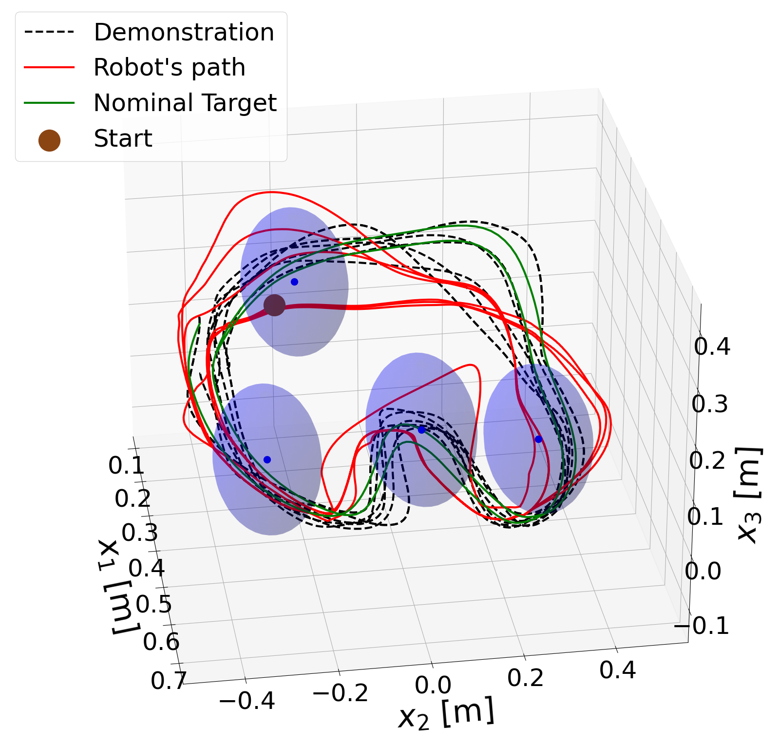
Figure 7: Franka Emika robot arm performing a periodic wiping task on a whiteboard. The purple spheres is the moving obstacle at different time.

5 Limitations & Future Work

The main contribution of this work is a NODE DS-based motion plan with an additive CBF and CLF-based correction term computed with respect to a time-varying target trajectory that ensures safety, stability, and when possible, task-completion. A limitation inherent to all CBF and CLF-based approaches is the risk of converging to a local minimum due to conflicting safety and task-completion constraints—this is a broader research question which falls beyond the scope of this paper. Our experiments are limited to using the Cartesian end-effector position $x\in\mathbb{R}^{3}$: future work will address this limitation by extending our approach to higher dimensional coordinate frames such as (a) orientation in $\mathcal{SO}(3)$ and position in $\mathbb{R}^{3}$ of the end-effector (Figueroa et al., 2020; Ravichandar and Dani, 2019; Zhang et al., 2022), (b) full pose of end-effector in $\mathcal{SE}(3)$ space (Urain et al., 2022), and (c) joint space (Shavit et al., 2018). Another limitation is our simple encoding of obstacles via sublevel sets of CBFs using closed-form expressions: to address this limitation, future work will explore novel (data-driven) representations of obstacles in joint space, e.g., via implicit distance functions (Koptev et al., 2023). Finally, since learning is performed offline, we can use a NN model that is more expensive to train than other DS-based motion planning methods (Khansari-Zadeh and Billard, 2011; Figueroa and Billard, 2022), which increases training time. Exploring different DS-based models that reduce training time without sacrificing expressivity is another important direction for future work.

Appendix A Illustration of disturbance rejection

In Fig. 9, we present a present a closer view of a disturbance rejection scenario given in Fig. 8, which is also given in Section 1. The paths generated using only the unconstrained Neural Ordinary Differential Equation (NODE) model, and the Control Lyapunov Function-NODE (CLF-NODE) approach is given in Fig. 9(a). The direction of the reference velocity computed using only NODE and the CLF-NODE is compared in Fig. 9(b).

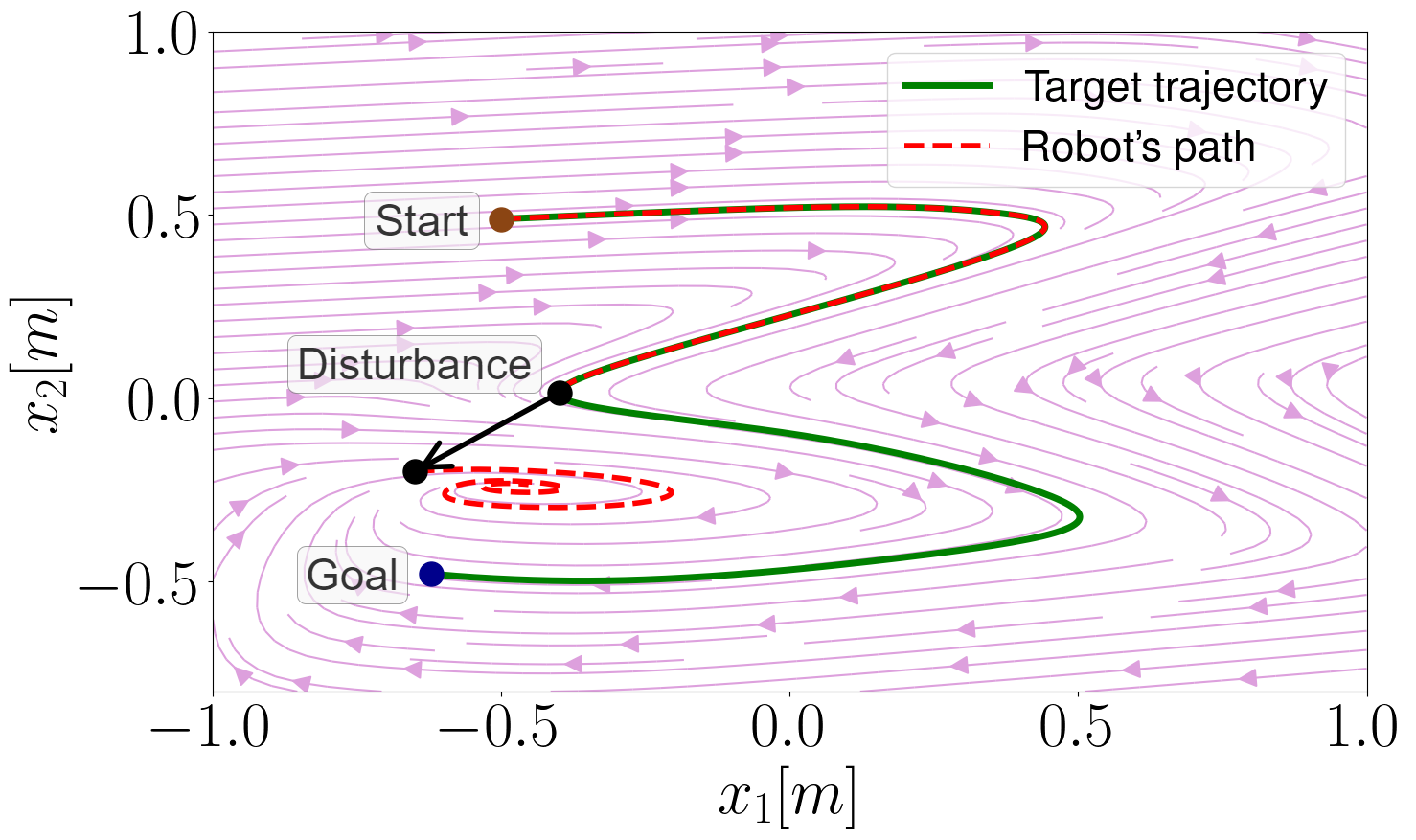
(a) Using standard NODE.

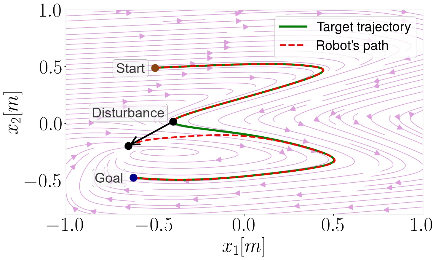
(b) Using CLF-NODE (ours).

Figure 8: An illustrative example of a spurious attractor when the robot’s path is guided by a DS-based motion plan in the presence of a disturbance.

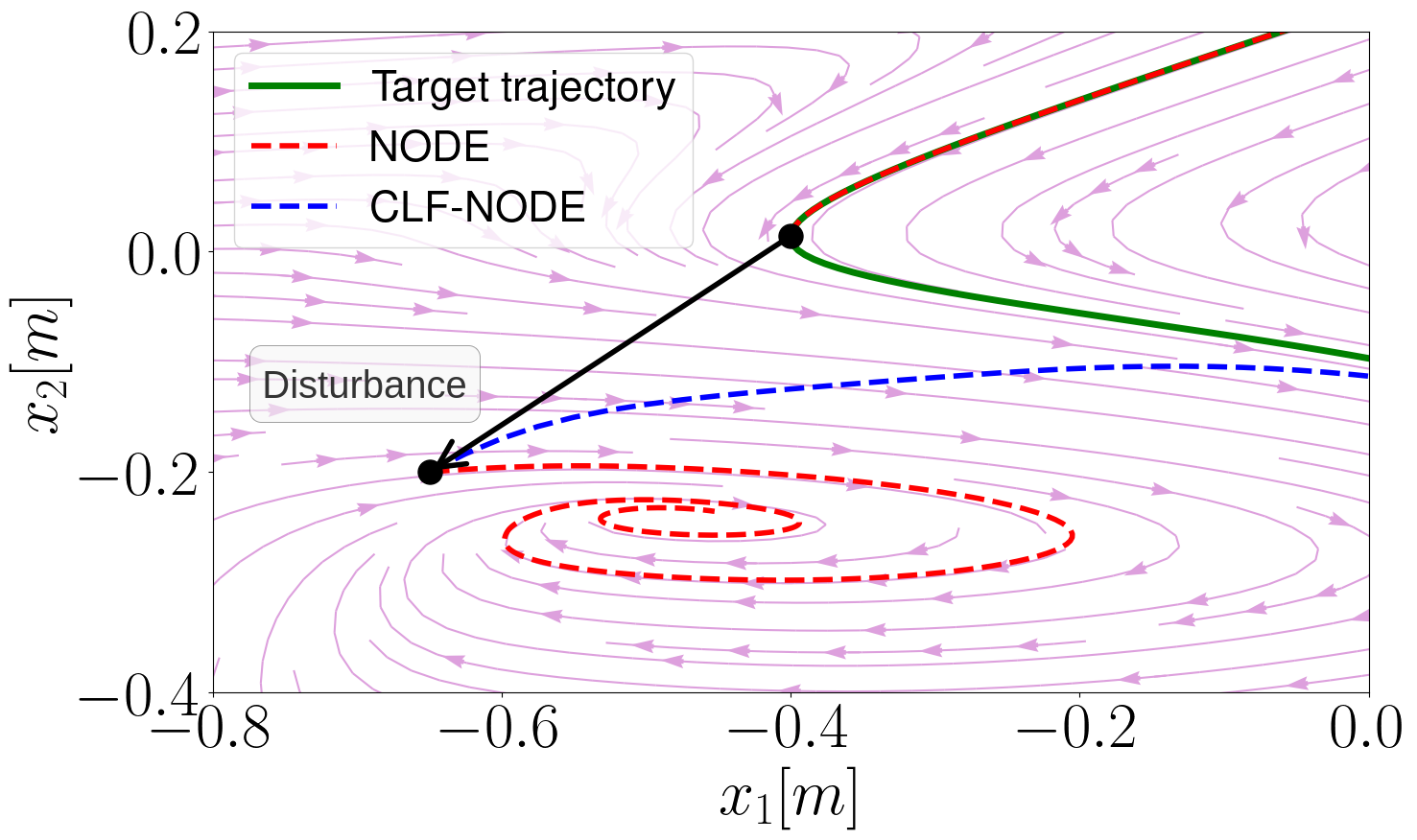
(a) Generated paths.

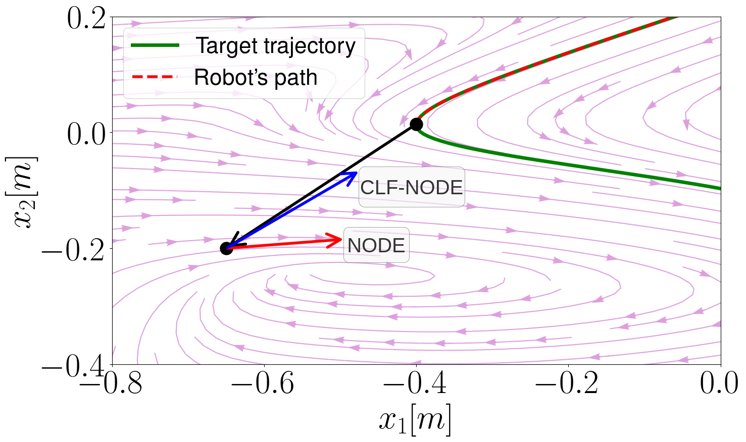
(b) Direction of generated reference velocity.

Figure 9: Closer view at the disturbance point of Fig. 8. Comparison of DS-based plan using only NODE, and with CLF-NODE.

Another example of tracking a target trajectory by a DS-based motion plan is given in Fig. 10. The scenario in Fig. 10(a) represents a path generated by the unconstrained DS-model using NODE that converge only to the goal. However, such a behaviour is also not ideal because the robot has to follow the target trajectory to wipe the desired space as given in Fig. 10(b).

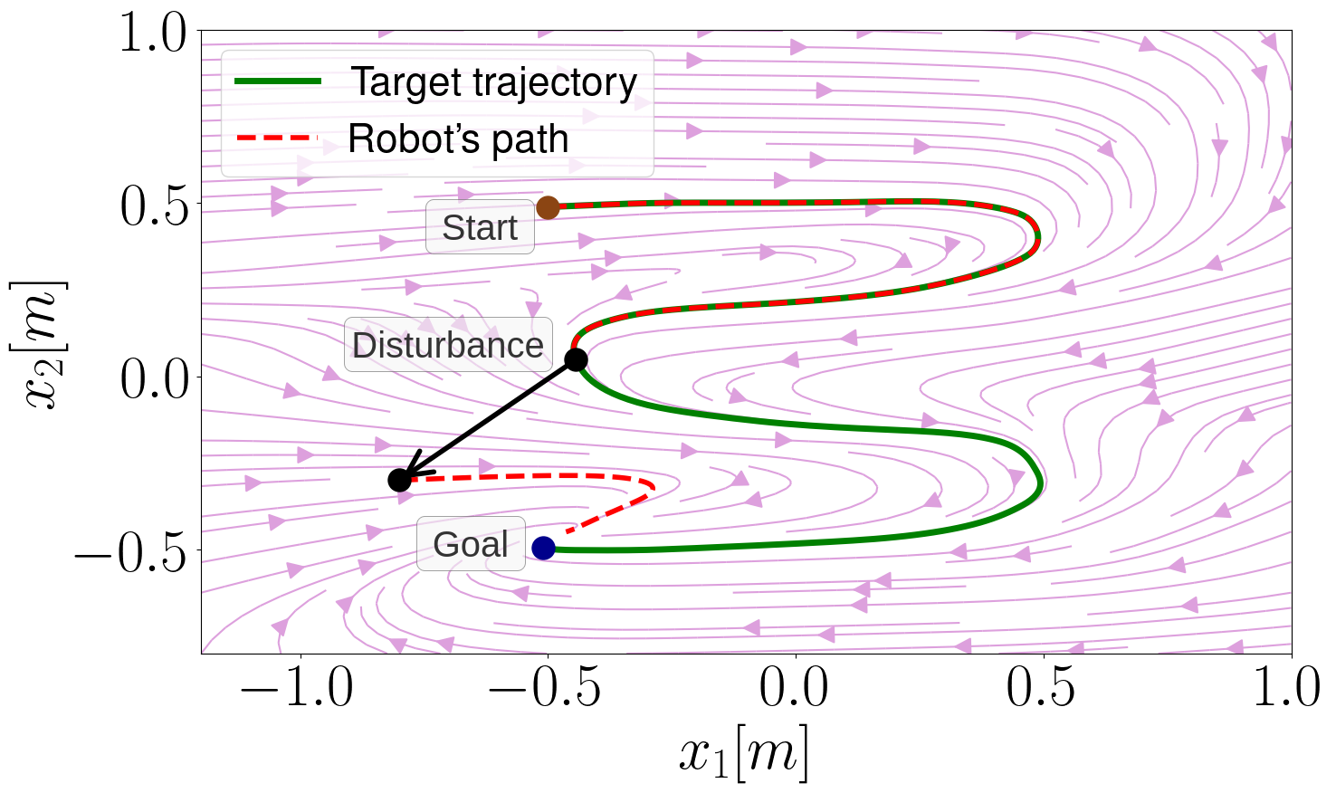
(a) Using standard NODE.

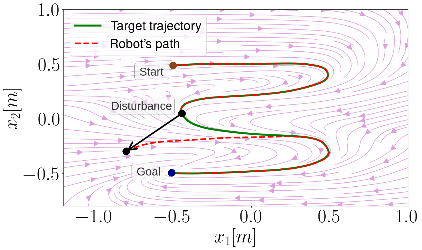
(b) Using CLF-NODE (ours).

Figure 10: An illustrative example of a robot’s path guided by a DS-based motion plan in the presence of a disturbance.

Appendix B Notes on implementation

Neural ODE We use a different modeling of the Neural ODE framework in (19), as opposed to (Chen et al., 2019; Rodriguez et al., 2022):

$$\frac{d\hat{x}(t)}{dt}=f_{\theta}(\hat{x}(t)),$$ (19)

where, $\hat{x}(t)$ is the state variable predicted by the NODE model $f_{\theta}(\cdot)$ at time $t$. Previous work (Rodriguez et al., 2022) assume an explicit input layer that transforms the input to a hidden state on which a differential equation is defined. The output is a transformation of the hidden state at each time $t$. In this work, there is no explicit input and output variables. Although such modeling allows us to learn more complex trajectories with a higher dimensional hidden state, the robot controller requires the reference velocity of the state variables $\dot{x}(t)$ for trajectory tracking (Billard et al., 2022b). Hence, we are interested in modeling the vector field of the physical state variable and not necessarily the hidden state.

Multiple tasks Our DS-based motion plan for a specific task defined by a nominal target trajectory $z^{*}(t)$ is given by an autonomous dynamical system:

$$\dot{x}=f(x),$$ (20)

where, $x$ is the state of the robot. We note that the model in (20) can incorporate scenarios where the robot has to switch between a finite number of tasks $N$. In such a case, we reformulate (20) such that $f(x,s(t))$ and $z^{*}(t,s(t))$ have an input signal $s(t)~{}\in~{}\{1,2,\ldots,N\}$ that commands the robot to follow a task $s(t)$ at any time $t$ when the robot is in motion. We design a vector field $f(\cdot)$ for each task using the task specific training data. At task execution, we manually command the robot using an external input signal $s(t)$ to switch between tasks and the corresponding learned DS models. We can also incorporate autonomous task switching mechanisms like (Khoramshahi and Billard, 2019) in our framework.

In the NODE framework, we solve the below empirical risk minimization problem for each task ${s\in\{1,2,\ldots,N\}}$:

$$\min_{\theta}\frac{1}{DT}\sum_{i=1}^{D}\sum_{k=1}^{T}\Bigl{\|}x_{i}^{s}(t_{k})-\hat{x}_{i}^{s}(t_{k})\Bigr{\|}_{2}^{2},$$ (21)

where, $\hat{x}_{i}^{s}(t_{k})$ is the state variable predicted by the model $f_{\theta(s)}$ at time $t_{k}$ for the $i^{th}$ demonstration of task $s\in\{1,2,\ldots,N\}$ . The training data for task $s$ is $\mathcal{D}_{s}:=\{\{x_{i}^{s}(t_{k})\}_{k=1}^{T}\}_{i=1}^{D}$. The weights of the model associated with task $s$ is $\theta(s)$. We note that switching between tasks using different models $\theta(s)$ could lead to non-smooth trajectories. We keep the problem of generating smooth switching strategies for future work.

The CLF optimization problem given below is also useful for scenarios where the robot has to switch between tasks.

$$u(x)=\operatorname*{argmin}_{v}\bigl{\|}v\bigr{\|}^{2}_{2}\quad\textnormal{s.t.} \nabla_{e}V(e)^{\top}\left(f_{\theta}(x)-\dot{x}^{*}+v\right)\leq-\alpha(V(e)).$$ (22)

Assume that the robot is following task $j$ with a learnt model $f_{\theta(j)}$ from time $t=0$. If we solve (22) for task $j$ at inference for every time $t$, the actual state of the robot $x(t)$ will be close to the target trajectory $x^{*}(t,j)$ that corresponds to task $j$, barring some process noise. Let at time $t=t_{k}$, an external input is commanding the robot to switch from task $j$ to task $k$ with a learnt model $f_{\theta(k)}$. Now, the state of the robot $x(t_{k})$ might be far away from the target trajectory $x^{*}(t,k)$ for the new task $k$. Since the model $f_{\theta(k)}$ is learnt only using demonstrations of task $k$, the model $f_{\theta(k)}$ alone will not guarantee convergence of $x(t)$ to $x^{*}(t,k)$. Hence, at time $t=t_{k}$, we switch to solving (22) with task $k$ so that the robot follows the model and target trajectory for task $k$. The CLF constraint in (22) will guarantee that the actual state of the robot $x(t)$ converges to the target trajectory of the new task $x^{*}(t,k)$.

Stability using CLF For the sake of completeness, we give the closed form expression to the optimization problem (22) that guarantees stability with respect to the time-varying target trajectory $x^{*}(t)$.

$$u(x)=\begin{cases}0,\ \textnormal{if}\ x=x^{*}\ \textnormal{(or)}\ \nabla_{e}V(e)^{\top}\left(f_{\theta}(x)-\dot{x}^{*}\right)\leq-\alpha(V(e))\\ -\left(\frac{\nabla_{e}V(e)^{\top}\left(f_{\theta}(x)-\dot{x}^{*}\right)+\alpha(V(e))}{\nabla_{e}V(e)^{\top}\nabla_{e}V(e)}\right)\nabla_{e}V(e),\ \textnormal{otherwise}.\end{cases}$$ (23)

Choosing Target point During deployment, given the current state $x$, target point $x^{*}$, and derivative at target point $\dot{x}^{*}$; we solve the CLF-CBF optimization problem given below at every time $t$.

$$(u(x),\_)=\operatorname*{argmin}_{\{v,\epsilon\}}\quad\bigl{\|}v\bigr{\|}^{2}_{2}+\lambda\epsilon^{2}\quad\textnormal{s.t.} \nabla_{x}B(x)^{\top}\left(f_{\theta}(x)+v\right)\geq-\gamma(B(x)),\forall\ x\in\mathcal{X},$$ (24)

$$\nabla_{e}V(e)^{\top}\left(f_{\theta}(x)-\dot{x}^{*}+v\right)\leq-\alpha(V(e))+\epsilon,\forall\ e\in\mathbb{R}^{d},$$

Then, we command the reference velocity $\dot{x}=f_{\theta}(x)+u(x)$ to the low level impedance controller. However, unanticipated disturbances and obstacles during task execution might perturb the robot away from the nominal target point $x^{*}$. Also, time synchronization might not be perfect between the different online computation blocks in the entire control flow. We remove the direct dependence of the target point $x^{*}$ on time $t$ by choosing $\pi(x)$ using Algorithm 2, which is also given in the main paper.

Input: $\mathcal{T}:=\{x^{*}(t_{k})\}_{k=1}^{T},f_{\theta}(\cdot),x,N$

Output: $\pi(x)$

$m\leftarrow\operatorname*{argmin}_{k\in\{1,2,\ldots,T\}}\big{\|}x-x^{*}(t_{k})\big{\|}_{2}$;

${\mathcal{T}_{N}:=\{x^{*}(t_{k})\ :\ k~{}\in~{}\{m,m+1,\ldots,\min(m+N,T)\}\}}$;

Solve (24) with parameters $\{x,y,f_{\theta}(y)\}$ for each $y\in\mathcal{T}_{N}$;

$\pi(x)\leftarrow\operatorname*{argmin}_{y\in\mathcal{T}_{N}}\big{\|}u(x,y,f_{\theta}(y))\big{\|}_{2}^{2}$;

Algorithm 2 Choose target point

The input to the algorithm is $\mathcal{T},f_{\theta},x,$ and a horizon length $N$ that describes how far to look forward along the target array to choose $\pi(x)$. In line 1, we choose the point $x^{*}(t_{m})$ in $\mathcal{T}$ that is closest to the current state of the robot. In line 2, we construct an array $\mathcal{T}_{N}$ of length at-most $N+1$ that contains $x^{*}(t_{m})$ and the next $N$ points along the target array $\mathcal{T}$. Then, we choose the target point $\pi(x)$ from $\mathcal{T}_{N}$ that results in the smallest norm of virtual control input when solving (24) amidst all points in $\mathcal{T}_{N}$. Finally, the virtual control input $u(x,\pi(x),f_{\theta}(\pi(x)))$ is used to compute the reference velocity $\dot{x}=f_{\theta}(x)+u(x)$.

Appendix C Further validation and results

LASA data set In Fig. 11, we compare the performance of our NODE model on four highly non-linear trajectories where existing approaches: SEDS (Khansari-Zadeh and Billard, 2011) and LPV-DS(Figueroa and Billard, 2022); either directly go to the target point or do not capture the entire shape. We also present the trajectories predicted by our model on other non-linear and multi modal shapes in Fig. 12. In Fig. 13(a) we present an additional disturbance rejection scenario by our CLF-NODE approach, and an obstacle avoidance scenario in Fig. 13(b). We model the obstacle as a circle in Fig. 13(b), where, the region outside the blue obstacle is the safe region $\mathcal{C}$ as defined for the Control Barrier Function (CBF). The safe region is described using the CBF $B(x)=\|x-c\|_{2}^{2}-r^{2}$, where $c$ and $r$ is the center and radius of the obstacle, respectively. We present the two scenarios in Fig. 14, where the robot switches from one mode to another during task execution. We use a linear form for the class $\mathcal{K}$ functions in (24): $\alpha(x)=k_{L}x,\gamma(x)=k_{B}x$; where, $k_{L}$ and $k_{B}$ are appropriate numerical constants for the CLF and CBF constraint, respectively. The forward looking horizon used is $N=3$ for Algorithm 2. We use $\lambda=900$ as the penalty term for the CLF-CBF QP.

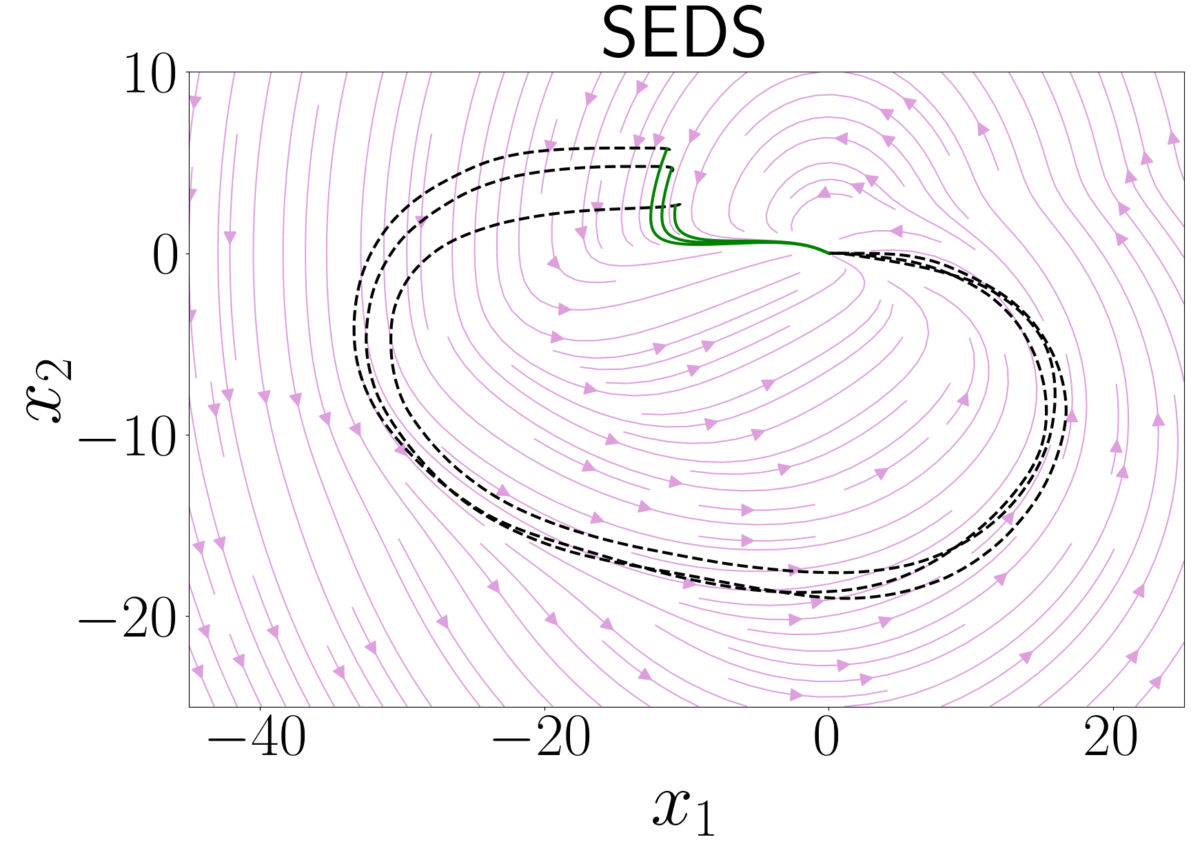
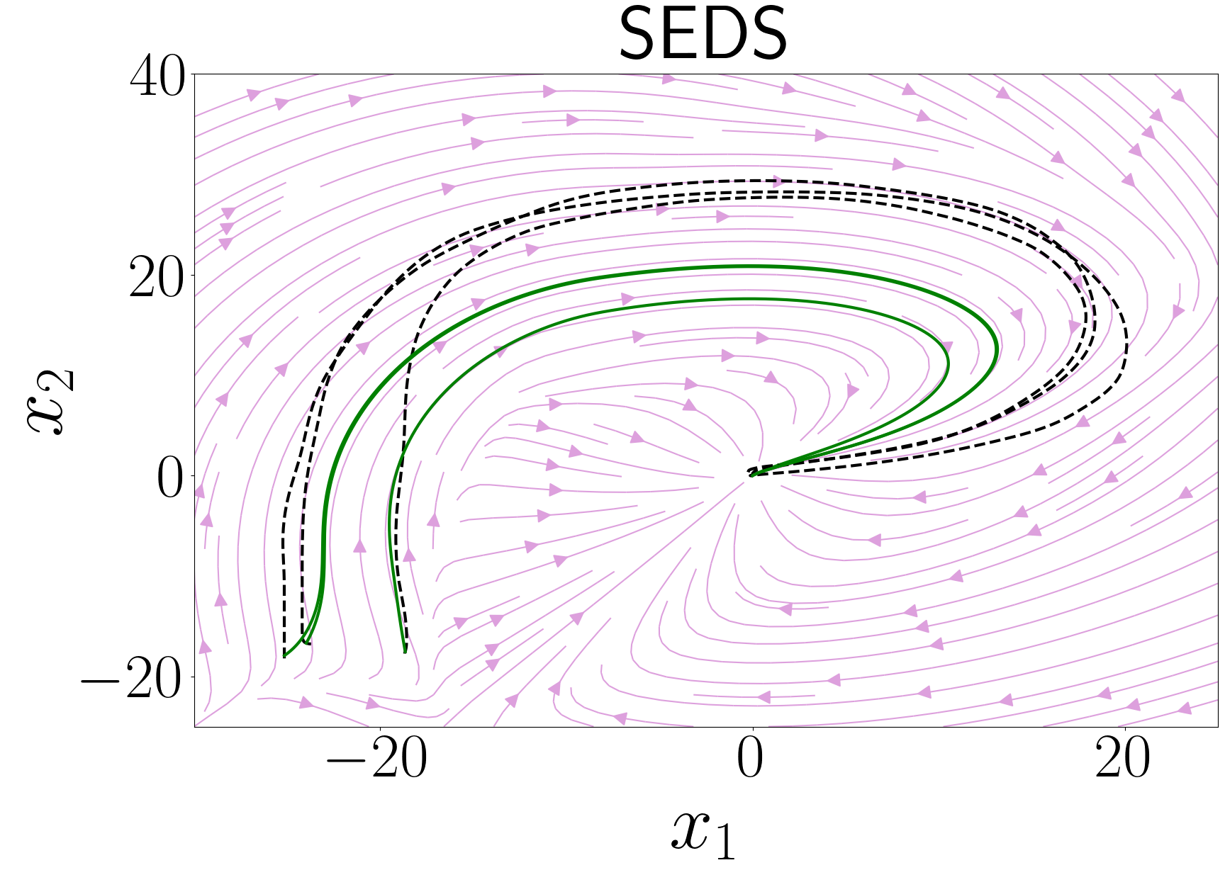
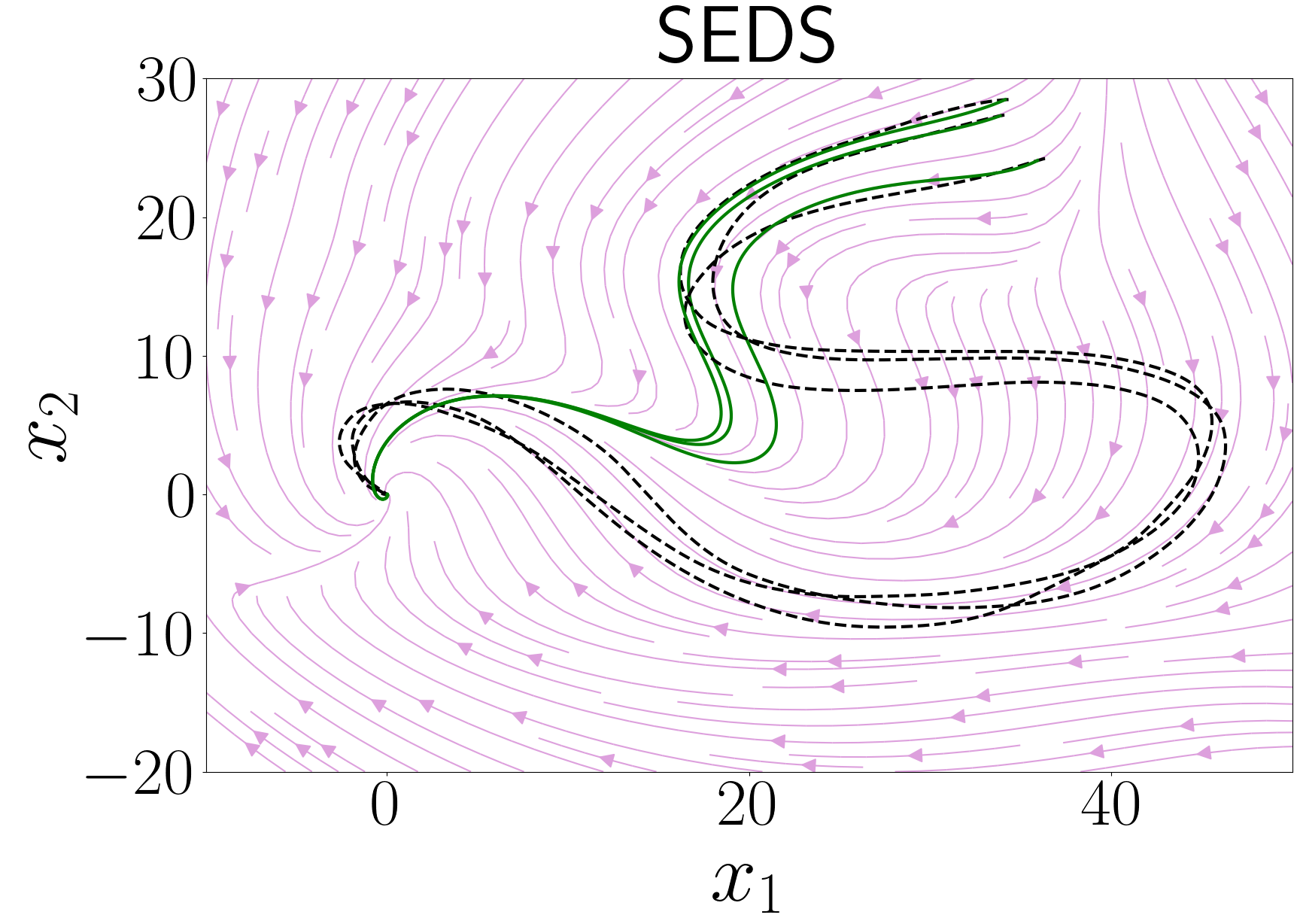
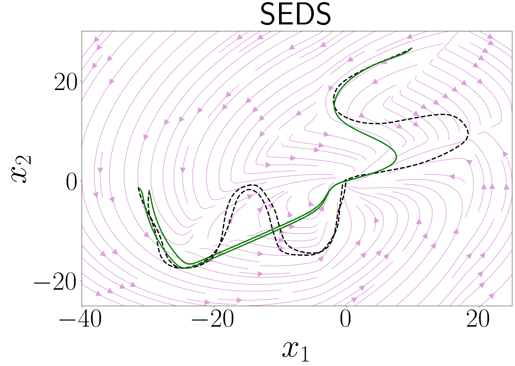
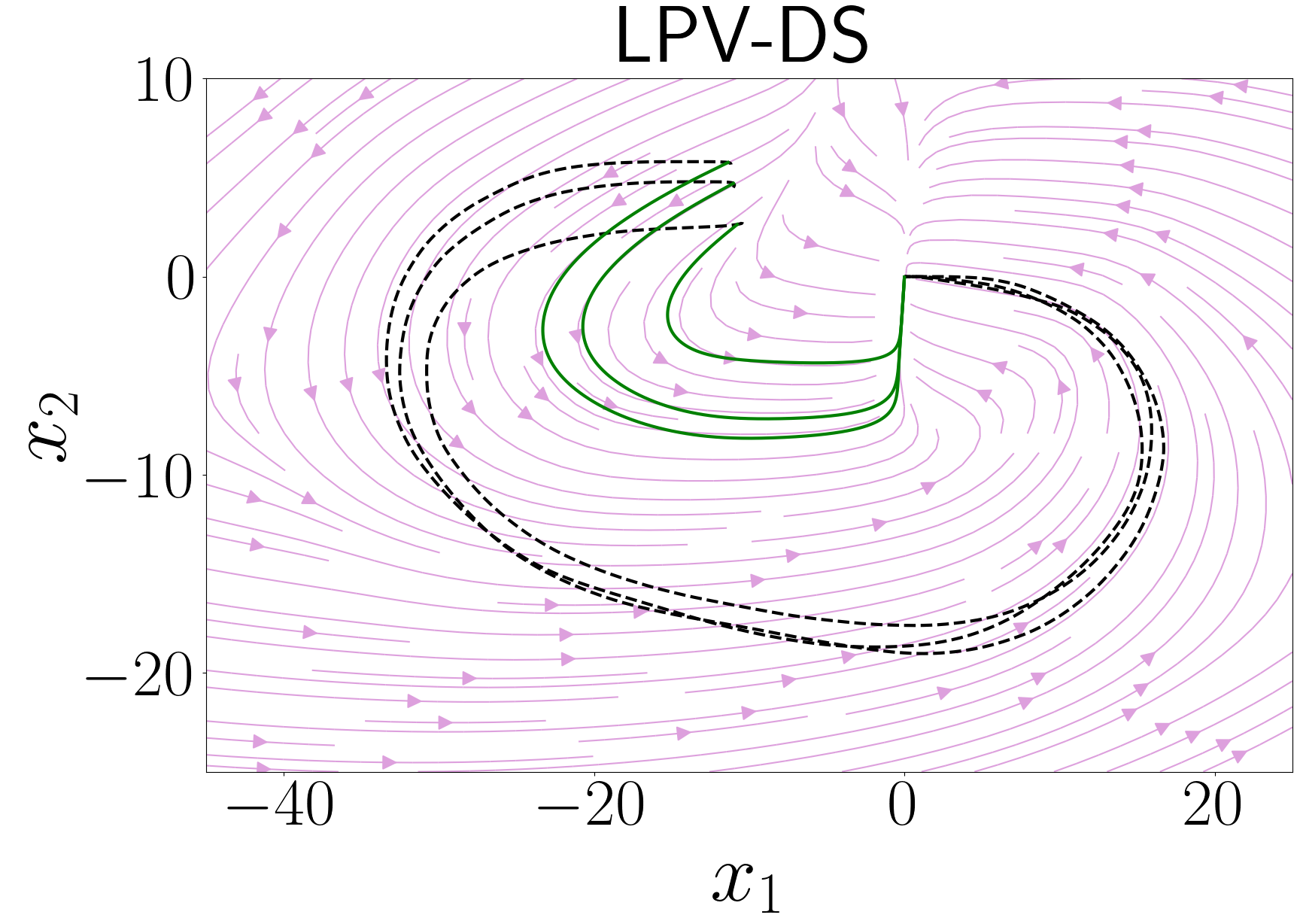
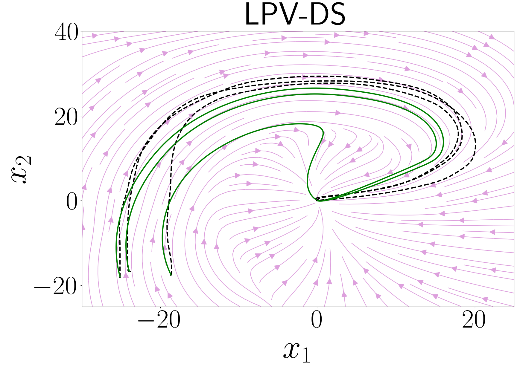
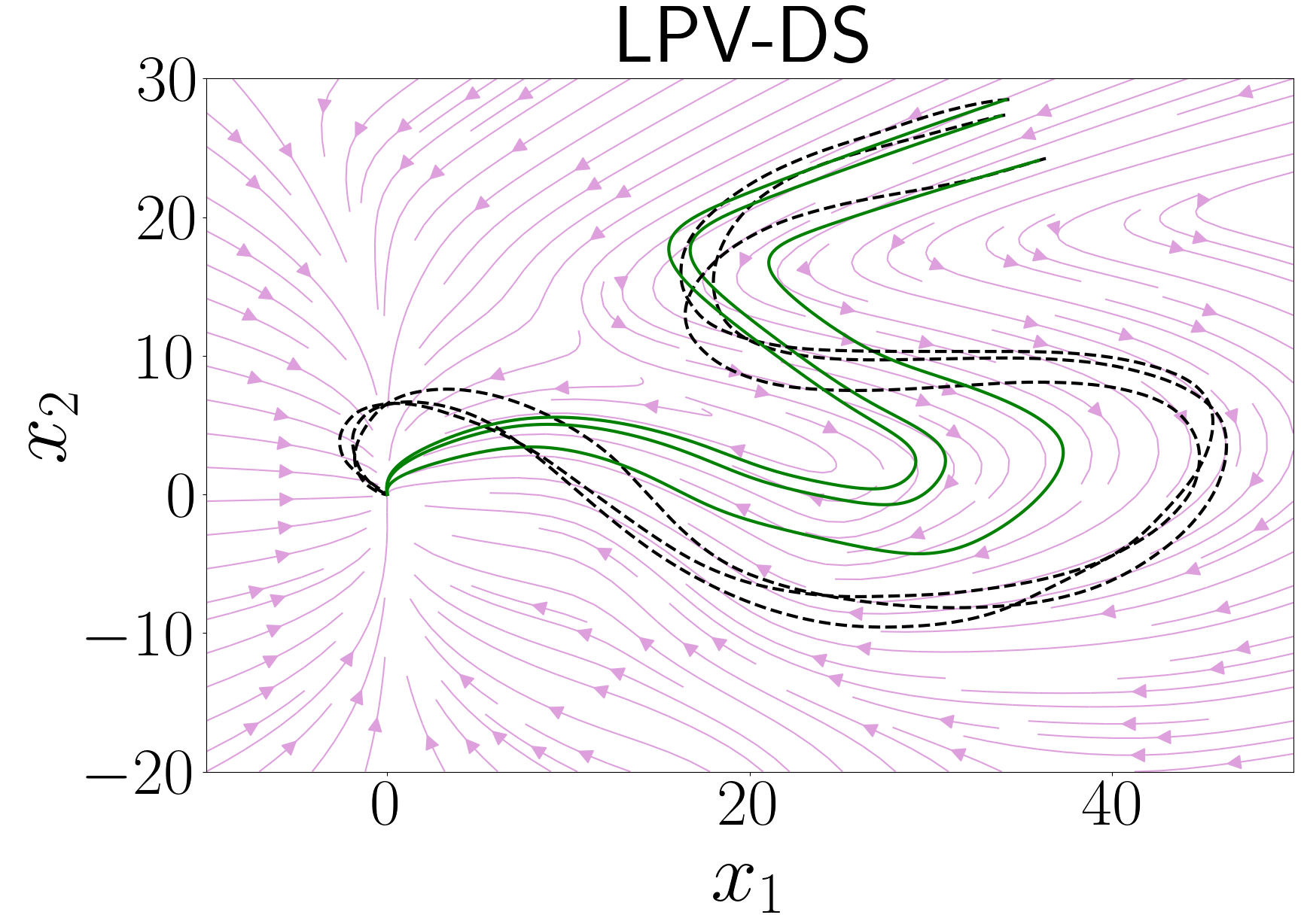
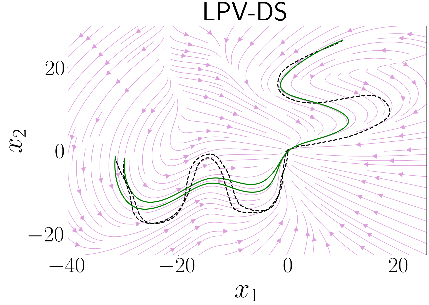
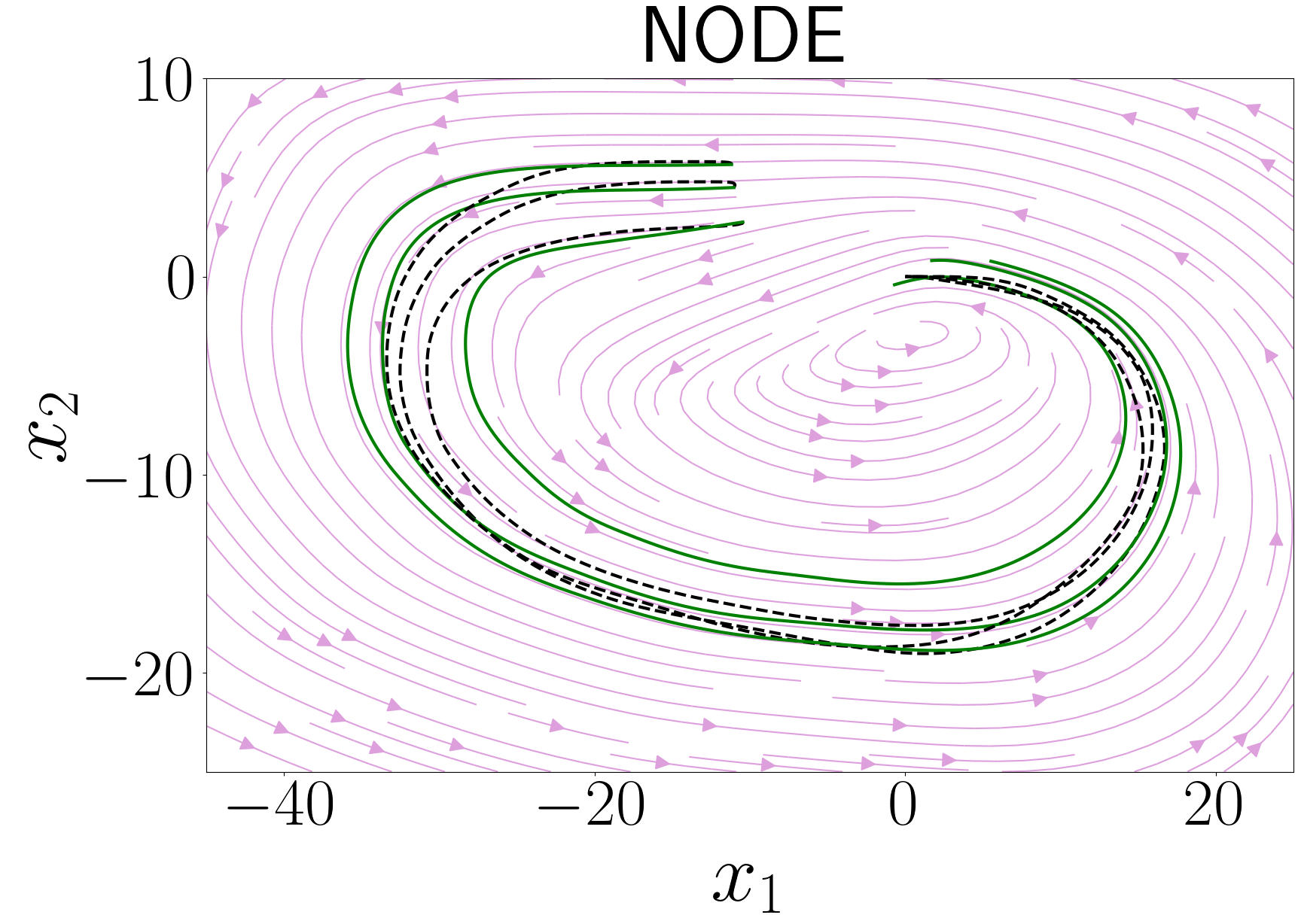
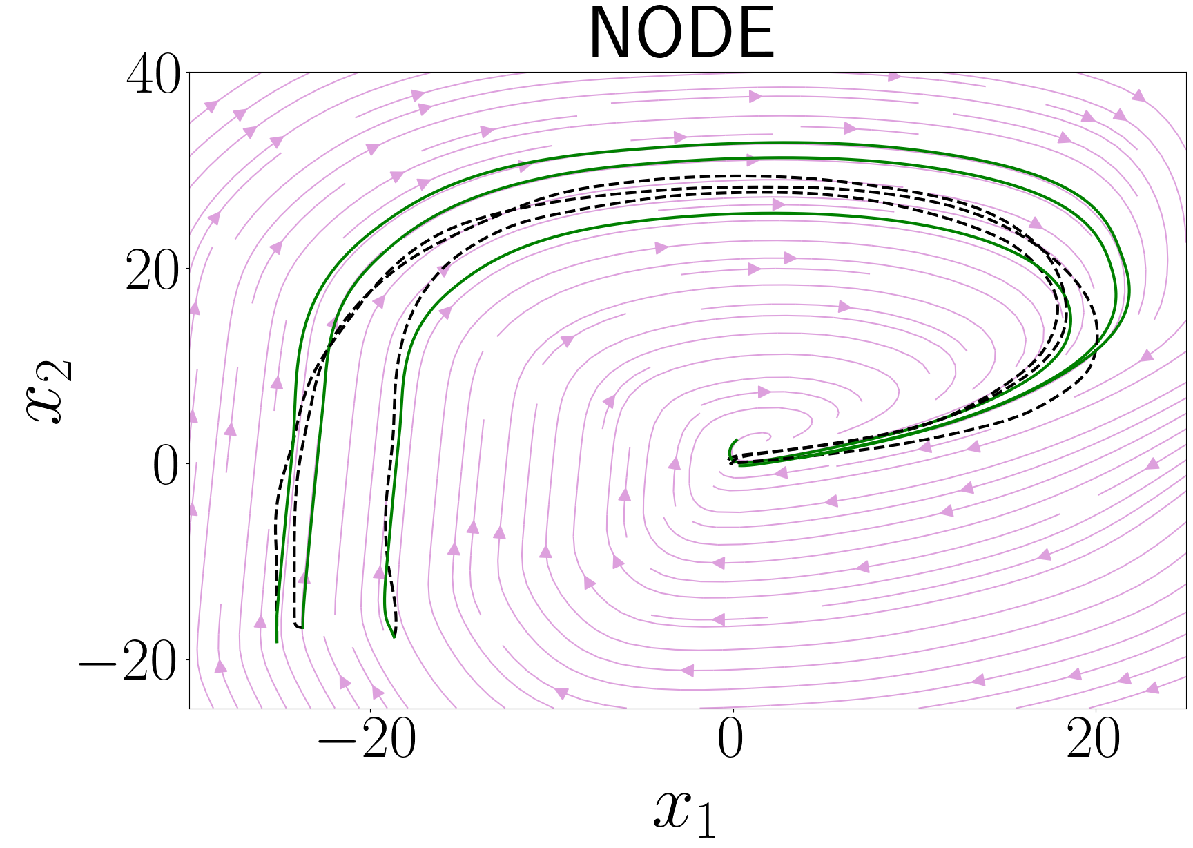
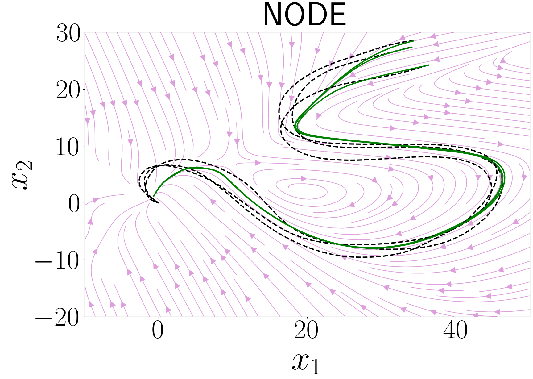
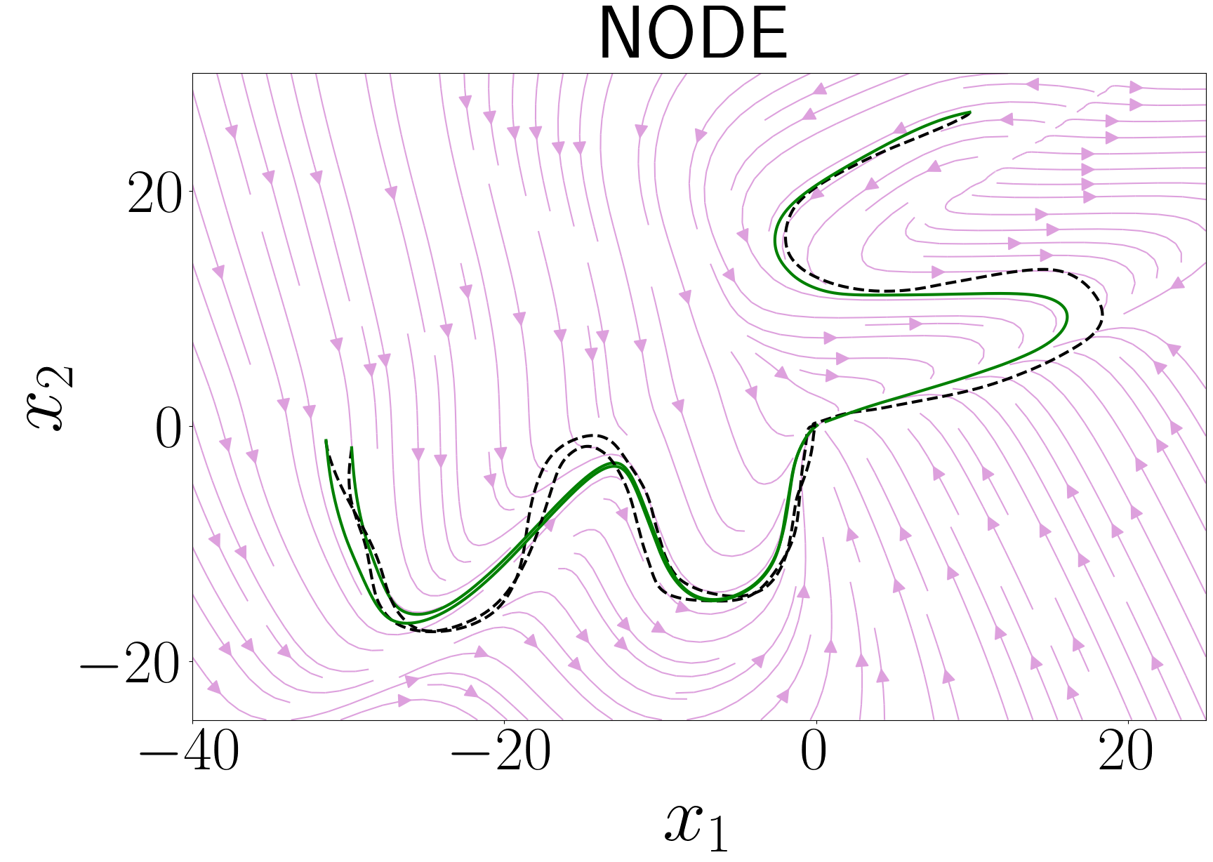
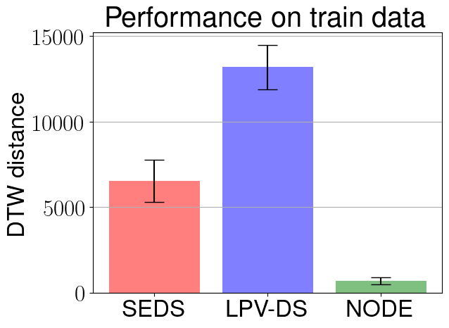
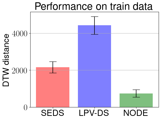
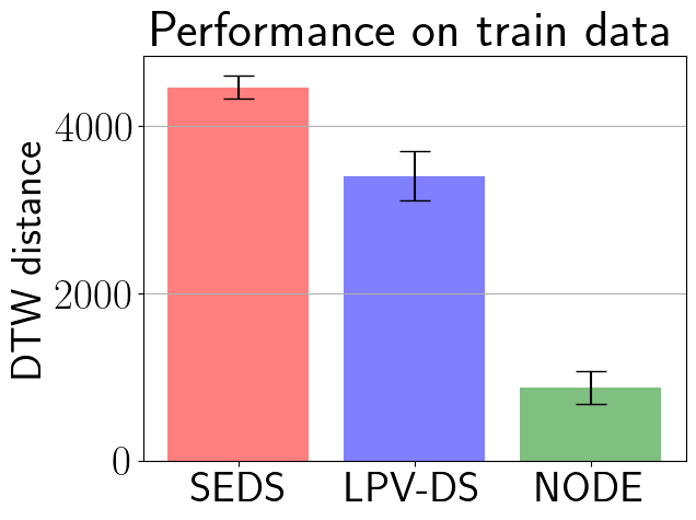
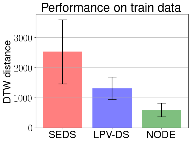
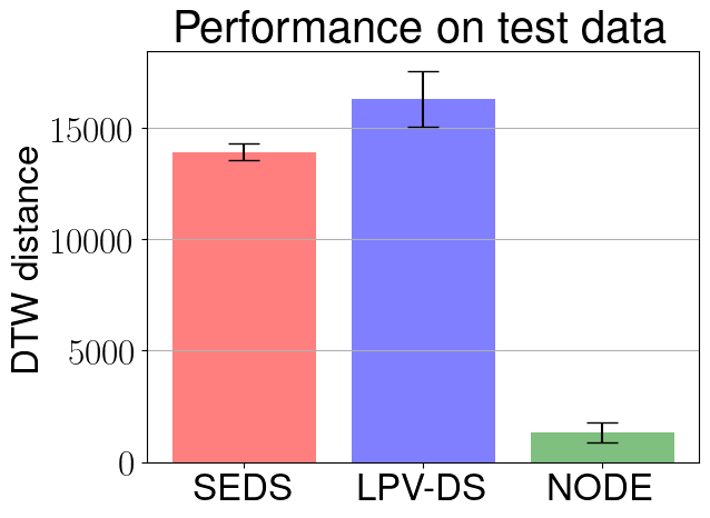
(a) DoubleBendedLine

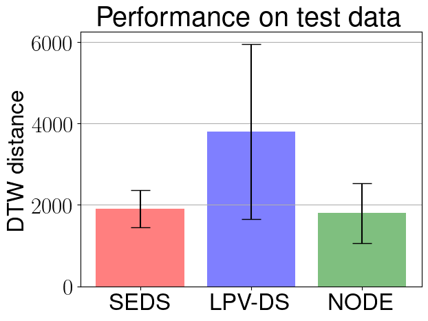
(b) PShape

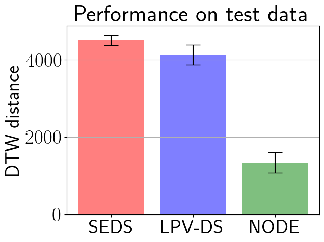
(c) Snake

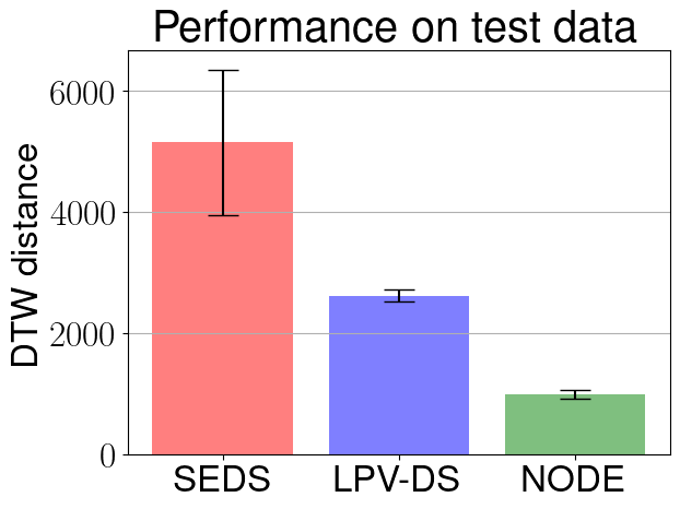
(d) MultiModels3

Figure 11: Trajectories predicted from the LASA test data set. The dashed black trajectories are from the data set. The solid green trajectories are predicted by the model. 1st row: Prediction from SEDS. 2nd row: Predictions from LPV-DS. 3rd row: Predictions by our Neural ODE (NODE) model. 4th row: DTW distance comparison on train data. 5th row: DTW distance comparison on test data.

(a) BendedLine

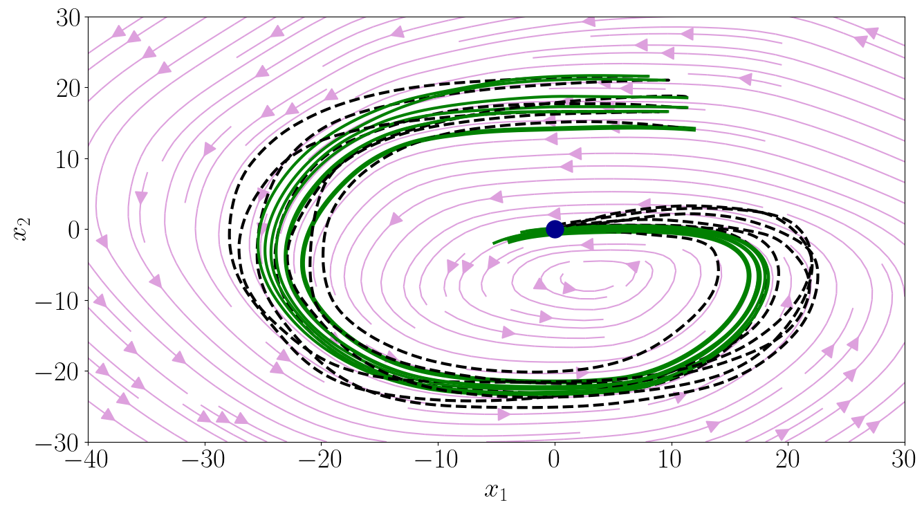
(b) GShape

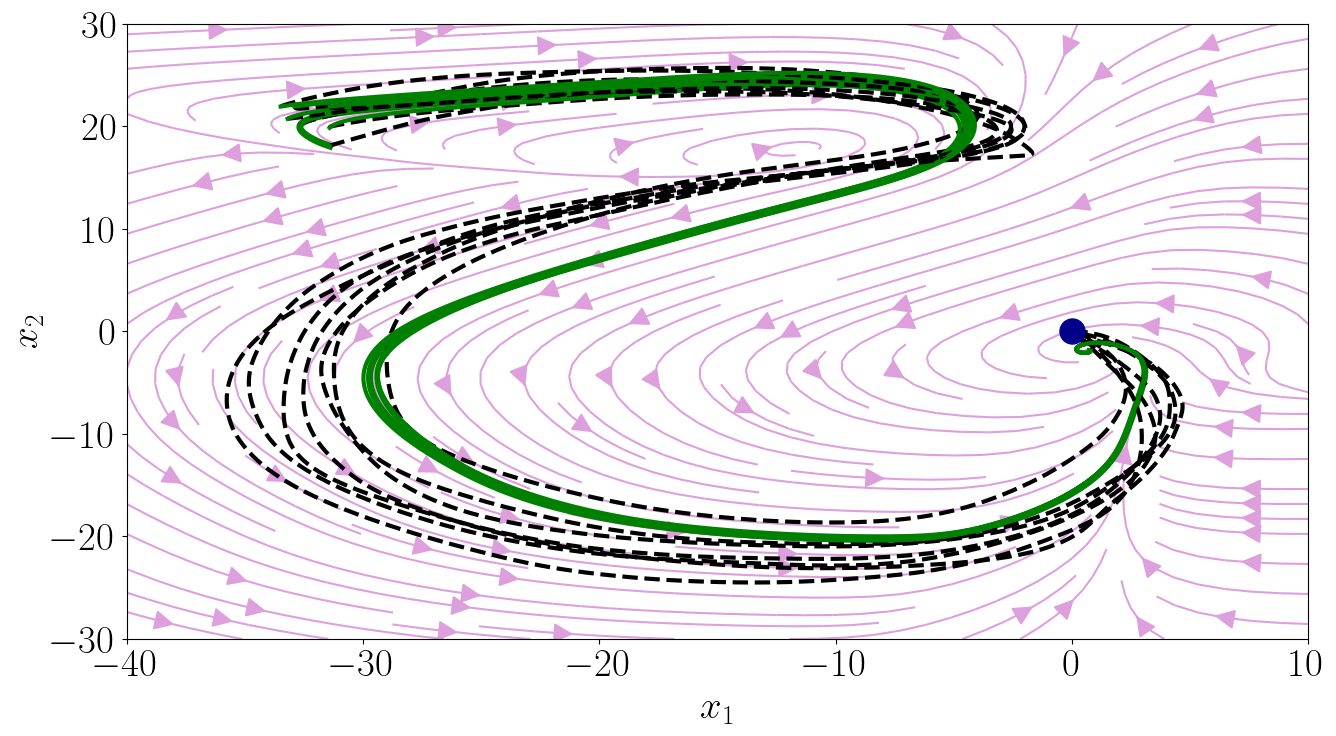
(c) heee

(d) NShape

(e) Leaf-1

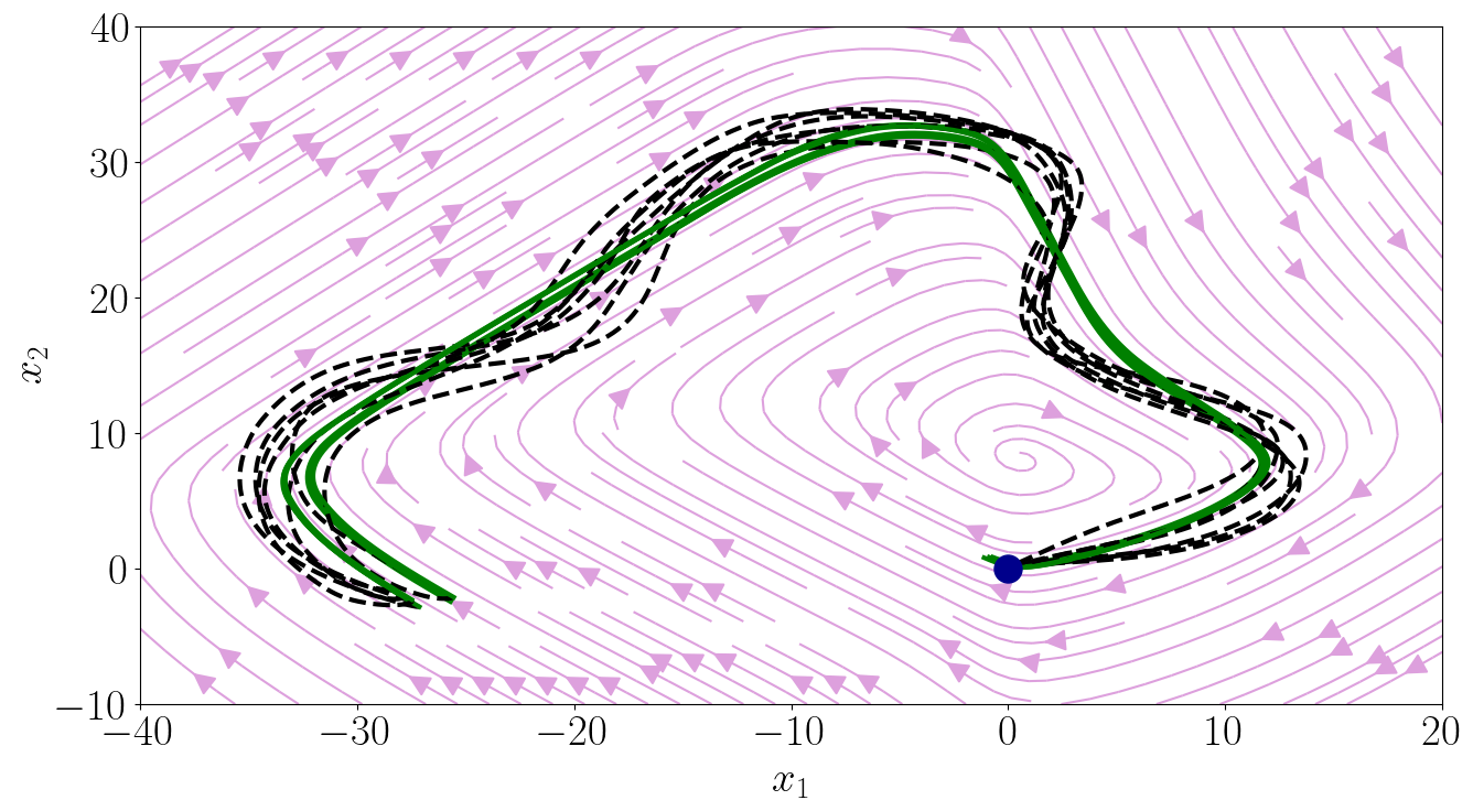
(f) Leaf-2

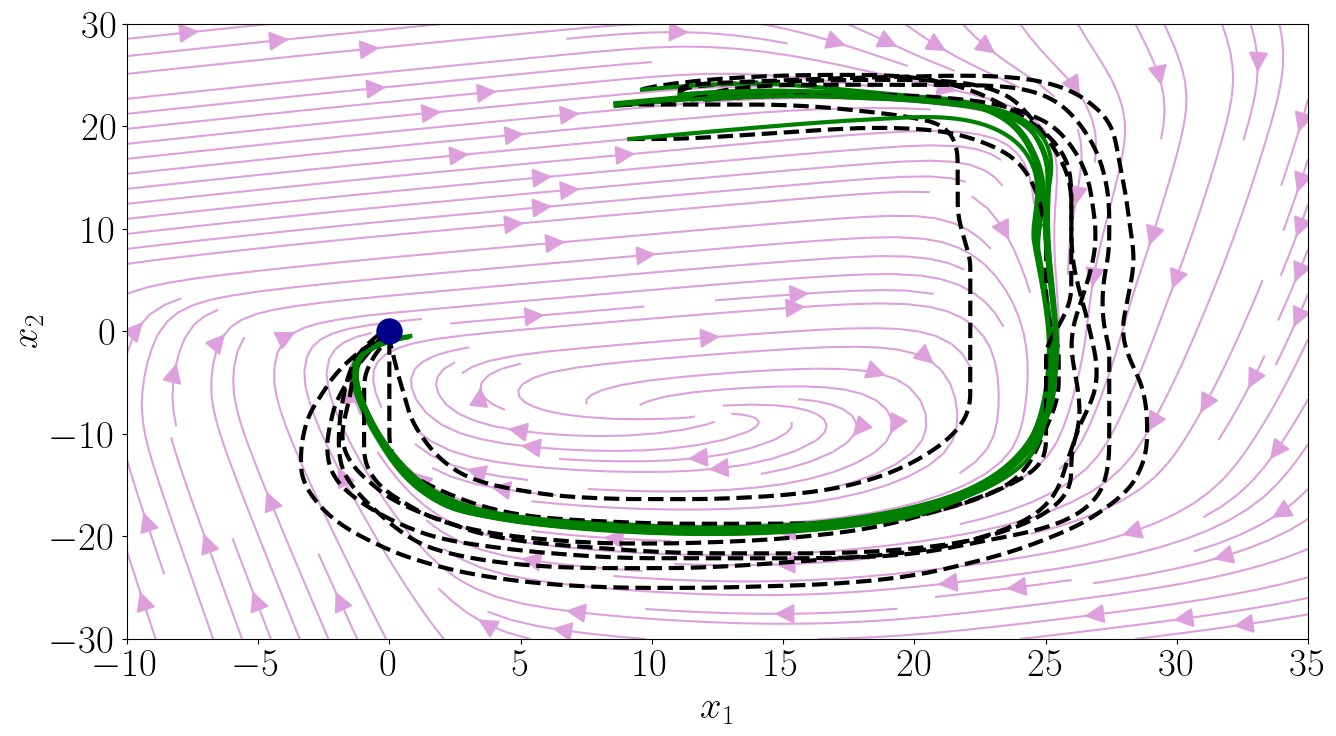
(g) JShape-2

(h) Spoon

(i) CShape

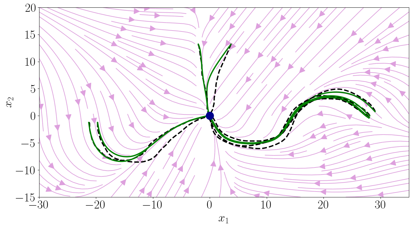
(j) MultiModels1

(k) MultiModels2

(l) MultiModels4

Figure 12: Trajectories predicted by the NODE model without any safety or stability constraints on some non-linear and multi modal trajectories from the LASA handwriting data set. The dashed black trajectories are from the data set. The solid green trajectories are predicted by our model.

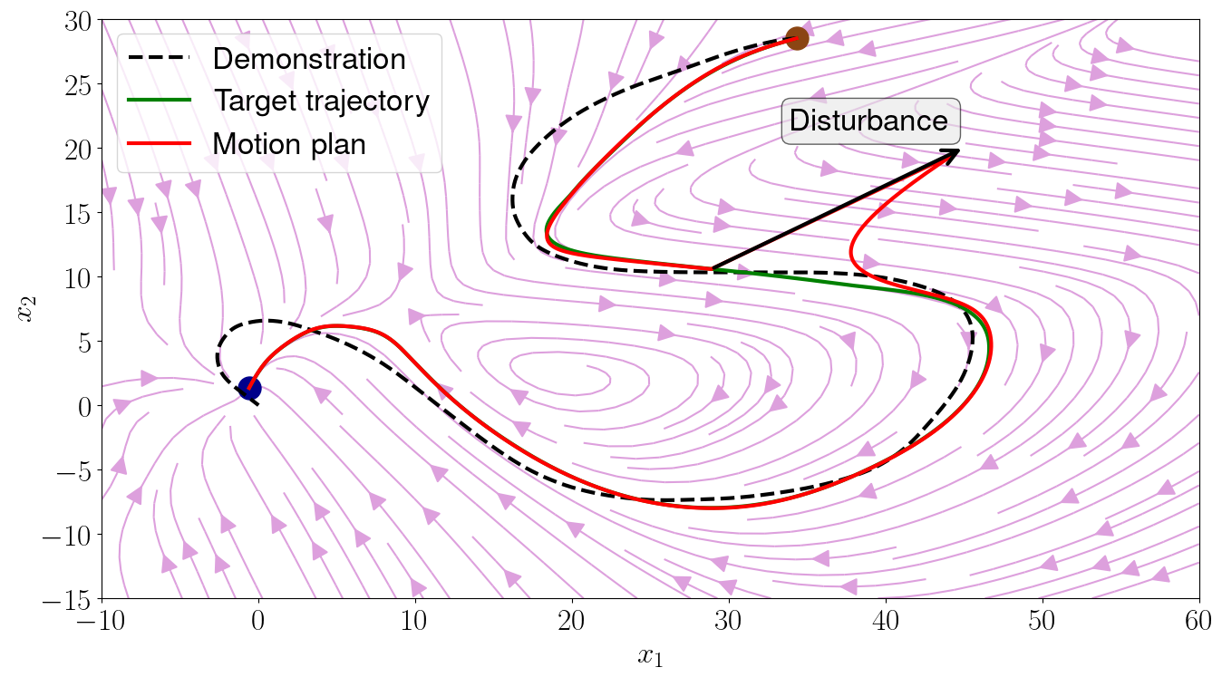
(a) Snake with disturbance

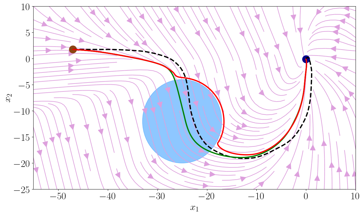
(b) Spoon with obstacle

Figure 13: Stable and safe motion plan generated by our CLF-NODE and CBF-CLF NODE, respectively. Brown dot is the initial point, and blue dot is the target point.

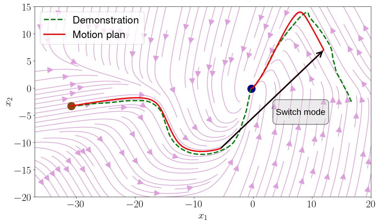
(a) MultiModels2

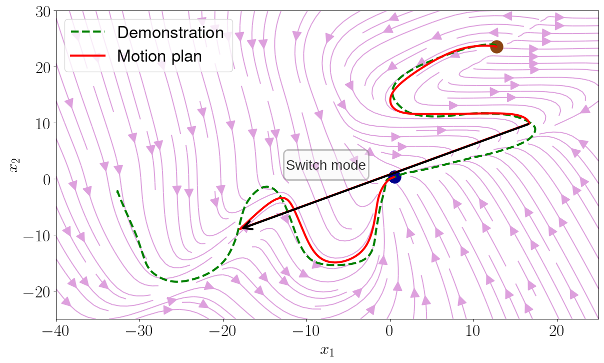
(b) MultiModels3

Figure 14: Motion plan generated by our method when switching between modes. Brown dot is the initial point, and blue dot is the target point.

Robot experiments We present the three dimensional trajectory and the snapshots of the Franka Emika robot arm performing a stirring task with a spoon in Fig. 15. We use 2 demonstrations and each has $300$ data samples. We parameterize the vector field $f_{\theta}(\cdot)$ as a Multi-Layer Perceptron with width = 64, depth = 3 for the stirring task, and width = 128, depth = 3 for the wiping tasks. At time $t=2$, the human perturbs the robot away from the nominal target trajectory to add something to the pan. The robot continues to follow the target trajectory even after the perturbation. We use the same linear form of the class $\mathcal{K}_{\infty}$ functions used for the LASA data set. The forward looking horizon used in Algorithm 2 is $N=3$ for the stirring task and $N=5$ for the wiping tasks. We use $\lambda=800$ as the penalty term for the CLF-CBF QP. We implemented both our training and online motion planning pipeline using JAX (Bradbury et al., 2018). We used the OSQP solver in JAXOPT (Blondel et al., 2021) to solve for the CLF-CBF QP and JIT compiled the entire code. Our online motion planning method runs at 1000 Hz: the same frequency as the low level passive DS impedance controller (Kronander and Billard, 2016b).

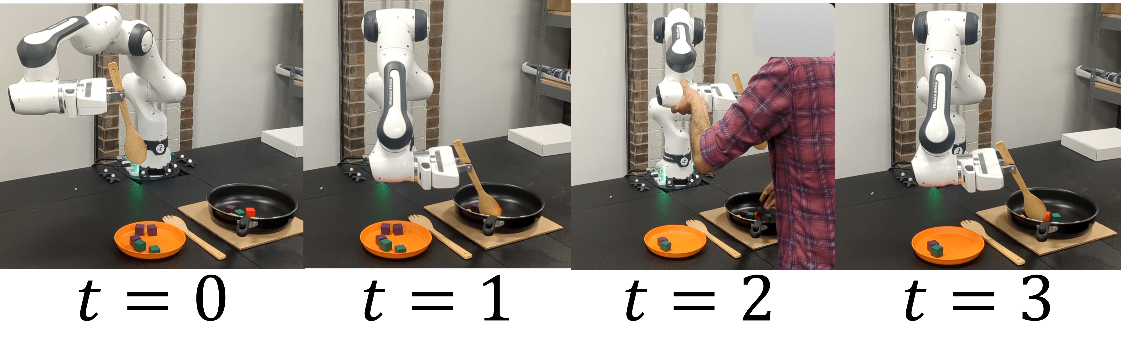
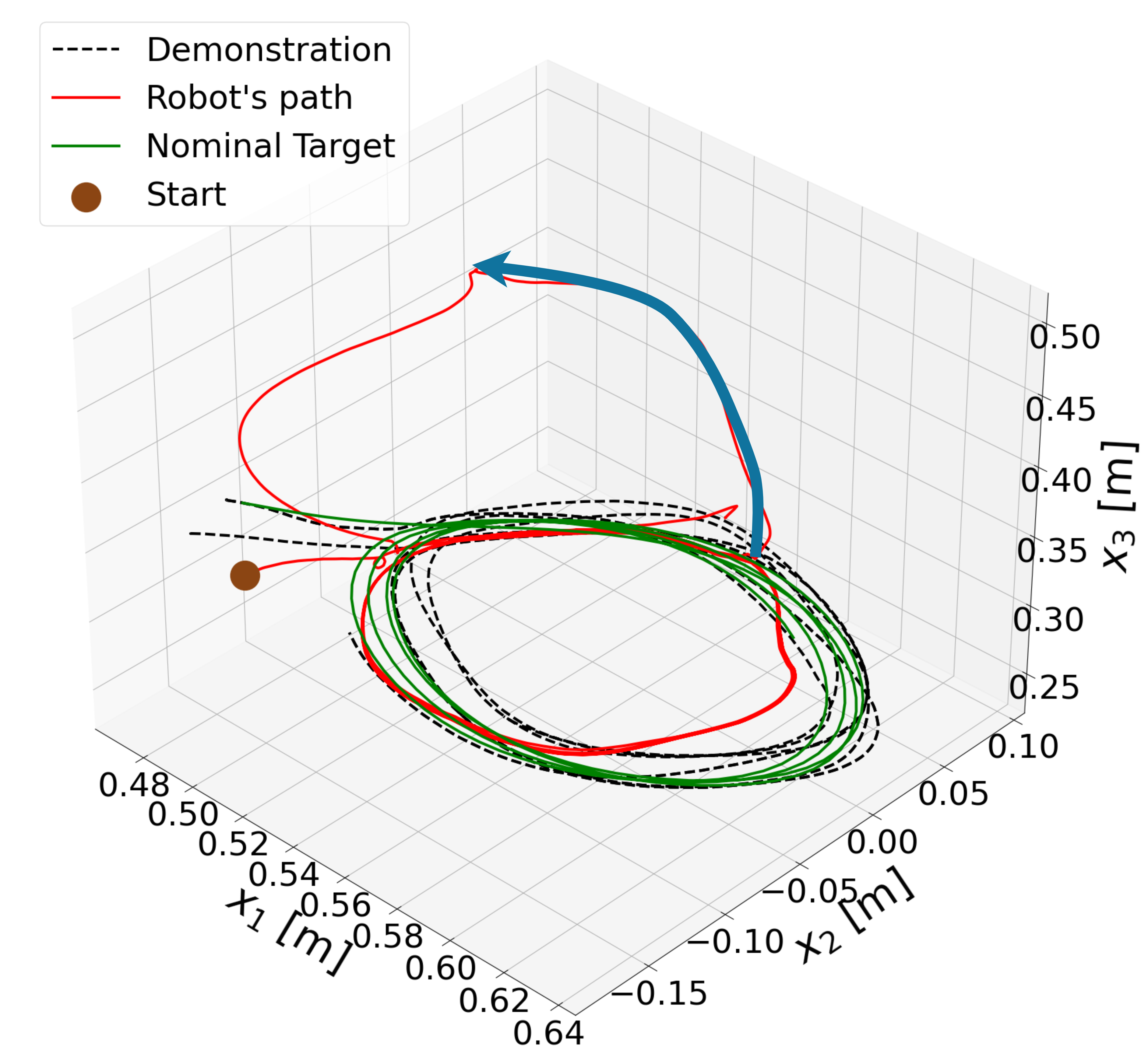
(a) Stirring a pan.

Figure 15: Franka Emika robot arm performing a periodic stirring task. The blue arrow denote the perturbation.

References

- Abbeel and Ng (2004) P. Abbeel and A. Y. Ng. Apprenticeship learning via inverse reinforcement learning. In Proceedings of the twenty-first international conference on Machine learning, page 1, 2004.
- Akgun and Subramanian (2011) B. Akgun and K. Subramanian. Robot learning from demonstration : Kinesthetic teaching vs . teleoperation. 2011.
- Ames et al. (2019) A. D. Ames, S. Coogan, M. Egerstedt, G. Notomista, K. Sreenath, and P. Tabuada. Control barrier functions: Theory and applications. In 2019 18th European control conference (ECC), pages 3420–3431. IEEE, 2019.
- Argall et al. (2009) B. D. Argall, S. Chernova, M. Veloso, and B. Browning. A survey of robot learning from demonstration. Robotics and autonomous systems, 57(5):469–483, 2009.
- Billard et al. (2022a) A. Billard, S. Mirrazavi, and N. Figueroa. Learning for Adaptive and Reactive Robot Control: A Dynamical Systems Approach. MIT Press, 2022a.
- Billard et al. (2022b) A. Billard, S. Mirrazavi, and N. Figueroa. Learning for Adaptive and Reactive Robot Control: A Dynamical Systems Approach. Mit Press, 2022b.
- Blondel et al. (2021) M. Blondel, Q. Berthet, M. Cuturi, R. Frostig, S. Hoyer, F. Llinares-López, F. Pedregosa, and J.-P. Vert. Efficient and modular implicit differentiation. arXiv preprint arXiv:2105.15183, 2021.
- Bradbury et al. (2018) J. Bradbury, R. Frostig, P. Hawkins, M. J. Johnson, C. Leary, D. Maclaurin, G. Necula, A. Paszke, J. VanderPlas, S. Wanderman-Milne, and Q. Zhang. JAX: composable transformations of Python+NumPy programs, 2018. URL http://github.com/google/jax.
- Butcher (1996) J. C. Butcher. A history of runge-kutta methods. Applied numerical mathematics, 20(3):247–260, 1996.
- Chen et al. (2020) R. T. Chen, B. Amos, and M. Nickel. Learning neural event functions for ordinary differential equations. arXiv preprint arXiv:2011.03902, 2020.
- Chen et al. (2019) R. T. Q. Chen, Y. Rubanova, J. Bettencourt, and D. Duvenaud. Neural ordinary differential equations, 2019.
- Figueroa and Billard (2018) N. Figueroa and A. Billard. A physically-consistent bayesian non-parametric mixture model for dynamical system learning. In A. Billard, A. Dragan, J. Peters, and J. Morimoto, editors, Proceedings of The 2nd Conference on Robot Learning, volume 87 of Proceedings of Machine Learning Research, pages 927–946. PMLR, 29–31 Oct 2018. URL https://proceedings.mlr.press/v87/figueroa18a.html.
- Figueroa and Billard (2022) N. Figueroa and A. Billard. Locally active globally stable dynamical systems: Theory, learning, and experiments. The International Journal of Robotics Research, 41(3):312–347, 2022.
- Figueroa et al. (2020) N. Figueroa, S. Faraji, M. Koptev, and A. Billard. A dynamical system approach for adaptive grasping, navigation and co-manipulation with humanoid robots. In 2020 IEEE International Conference on Robotics and Automation (ICRA), pages 7676–7682, 2020. doi: 10.1109/ICRA40945.2020.9197038.
- Haber and Ruthotto (2017) E. Haber and L. Ruthotto. Stable architectures for deep neural networks. Inverse problems, 34(1):014004, 2017.
- Hoffmann et al. (2009) H. Hoffmann, P. Pastor, D.-H. Park, and S. Schaal. Biologically-inspired dynamical systems for movement generation: Automatic real-time goal adaptation and obstacle avoidance. In 2009 IEEE international conference on robotics and automation, pages 2587–2592. IEEE, 2009.
- Ijspeert et al. (2013) A. J. Ijspeert, J. Nakanishi, H. Hoffmann, P. Pastor, and S. Schaal. Dynamical movement primitives: learning attractor models for motor behaviors. Neural computation, 25(2):328–373, 2013.
- Jaquier et al. (2019) N. Jaquier, D. Ginsbourger, and S. Calinon. Learning from demonstration with model-based gaussian process. arxiv preprint arxiv: 191005005. 2019.
- Khalil (2015) H. K. Khalil. Nonlinear control, volume 406. Pearson New York, 2015.
- Khansari-Zadeh and Billard (2011) S. M. Khansari-Zadeh and A. Billard. Learning stable nonlinear dynamical systems with gaussian mixture models. IEEE Transactions on Robotics, 27(5):943–957, 2011.
- Khansari-Zadeh and Billard (2012) S. M. Khansari-Zadeh and A. Billard. A dynamical system approach to realtime obstacle avoidance. Autonomous Robots, 32:433–454, 2012.
- Khansari-Zadeh and Billard (2014) S. M. Khansari-Zadeh and A. Billard. Learning control lyapunov function to ensure stability of dynamical system-based robot reaching motions. Robotics and Autonomous Systems, 62(6):752–765, 2014.
- Khoramshahi and Billard (2019) M. Khoramshahi and A. Billard. A dynamical system approach to task-adaptation in physical human–robot interaction. Autonomous Robots, 43:927–946, 2019.
- Kidger (2022) P. Kidger. On neural differential equations. arXiv preprint arXiv:2202.02435, 2022.
- Koptev et al. (2023) M. Koptev, N. Figueroa, and A. Billard. Neural joint space implicit signed distance functions for reactive robot manipulator control. IEEE Robotics and Automation Letters, 8(2):480–487, 2023. doi: 10.1109/LRA.2022.3227860.
- Kronander and Billard (2016a) K. Kronander and A. Billard. Passive interaction control with dynamical systems. IEEE Robotics and Automation Letters, 1(1):106–113, 2016a. doi: 10.1109/LRA.2015.2509025.
- Kronander and Billard (2016b) K. Kronander and A. Billard. Passive interaction control with dynamical systems. IEEE Robotics and Automation Letters, 1(1):106–113, 2016b. doi: 10.1109/LRA.2015.2509025.
- Lukoševičius and Jaeger (2009) M. Lukoševičius and H. Jaeger. Reservoir computing approaches to recurrent neural network training. Computer science review, 3(3):127–149, 2009.
- Mattingley and Boyd (2012) J. Mattingley and S. Boyd. Cvxgen: A code generator for embedded convex optimization. Optimization and Engineering, 13:1–27, 2012.
- Nakanishi et al. (2004) J. Nakanishi, J. Morimoto, G. Endo, G. Cheng, S. Schaal, and M. Kawato. Learning from demonstration and adaptation of biped locomotion. Robotics and autonomous systems, 47(2-3):79–91, 2004.
- Osa et al. (2018) T. Osa, J. Pajarinen, G. Neumann, J. A. Bagnell, P. Abbeel, J. Peters, et al. An algorithmic perspective on imitation learning. Foundations and Trends® in Robotics, 7(1-2):1–179, 2018.
- Priess et al. (2014) M. C. Priess, J. Choi, and C. Radcliffe. The inverse problem of continuous-time linear quadratic gaussian control with application to biological systems analysis. In Dynamic Systems and Control Conference, volume 46209, page V003T42A004. American Society of Mechanical Engineers, 2014.
- Purwar et al. (2008) S. Purwar, I. N. Kar, and A. N. Jha. Adaptive output feedback tracking control of robot manipulators using position measurements only. Expert systems with applications, 34(4):2789–2798, 2008.
- Ravichandar and Dani (2019) H. C. Ravichandar and A. Dani. Learning position and orientation dynamics from demonstrations via contraction analysis. Autonomous Robots, 43(4):897–912, 2019.
- Ravichandar et al. (2017) H. C. Ravichandar, I. Salehi, and A. P. Dani. Learning partially contracting dynamical systems from demonstrations. In CoRL, pages 369–378, 2017.
- Reinhart and Steil (2011) R. F. Reinhart and J. J. Steil. Neural learning and dynamical selection of redundant solutions for inverse kinematic control. In 2011 11th IEEE-RAS International Conference on Humanoid Robots, pages 564–569. IEEE, 2011.
- Robey et al. (2020) A. Robey, H. Hu, L. Lindemann, H. Zhang, D. V. Dimarogonas, S. Tu, and N. Matni. Learning control barrier functions from expert demonstrations. In 2020 59th IEEE Conference on Decision and Control (CDC), pages 3717–3724. IEEE, 2020.
- Rodriguez et al. (2022) I. D. J. Rodriguez, A. Ames, and Y. Yue. Lyanet: A lyapunov framework for training neural odes. In International Conference on Machine Learning, pages 18687–18703. PMLR, 2022.
- Ross et al. (2011) S. Ross, G. Gordon, and D. Bagnell. A reduction of imitation learning and structured prediction to no-regret online learning. In Proceedings of the fourteenth international conference on artificial intelligence and statistics, pages 627–635. JMLR Workshop and Conference Proceedings, 2011.
- Salvador and Chan (2007) S. Salvador and P. Chan. Toward accurate dynamic time warping in linear time and space. Intelligent Data Analysis, 11(5):561–580, 2007.
- Schaal (2006) S. Schaal. Dynamic movement primitives-a framework for motor control in humans and humanoid robotics. Adaptive motion of animals and machines, pages 261–280, 2006.
- Shavit et al. (2018) Y. Shavit, N. Figueroa, S. S. M. Salehian, and A. Billard. Learning augmented joint-space task-oriented dynamical systems: A linear parameter varying and synergetic control approach. IEEE Robotics and Automation Letters, 3(3):2718–2725, 2018. doi: 10.1109/LRA.2018.2833497.
- Ude et al. (2010) A. Ude, A. Gams, T. Asfour, and J. Morimoto. Task-specific generalization of discrete and periodic dynamic movement primitives. IEEE Transactions on Robotics, 26(5):800–815, 2010.
- Urain et al. (2020) J. Urain, M. Ginesi, D. Tateo, and J. Peters. Imitationflow: Learning deep stable stochastic dynamic systems by normalizing flows. In 2020 IEEE/RSJ International Conference on Intelligent Robots and Systems (IROS), pages 5231–5237. IEEE, 2020.
- Urain et al. (2022) J. Urain, D. Tateo, and J. Peters. Learning stable vector fields on lie groups. IEEE Robotics and Automation Letters, 7(4):12569–12576, 2022. doi: 10.1109/LRA.2022.3219019.
- Wang et al. (2022) Y. Wang, N. Figueroa, S. Li, A. Shah, and J. Shah. Temporal logic imitation: Learning plan-satisficing motion policies from demonstrations. In 6th Annual Conference on Robot Learning, 2022. URL https://openreview.net/forum?id=ndYsaoyzCWv.
- Xiao et al. (2020) B. Xiao, L. Cao, S. Xu, and L. Liu. Robust tracking control of robot manipulators with actuator faults and joint velocity measurement uncertainty. IEEE/ASME Transactions on Mechatronics, 25(3):1354–1365, 2020. doi: 10.1109/TMECH.2020.2975117.
- Yang et al. (2022) J. Yang, J. Zhang, C. Settle, A. Rai, R. Antonova, and J. Bohg. Learning periodic tasks from human demonstrations. In 2022 International Conference on Robotics and Automation (ICRA), pages 8658–8665. IEEE, 2022.
- Zhang et al. (2022) J. Zhang, H. B. Mohammadi, and L. Rozo. Learning riemannian stable dynamical systems via diffeomorphisms. In 6th Annual Conference on Robot Learning, 2022.