# FashionMNIST Labels per class	1	2	3	4	5	4000
Laplace/LP [56]	18.4 (7.3)	32.5 (8.2)	44.0 (8.6)	52.2 (6.2)	57.9 (6.7)	85.8 (0.0)
Poisson [12]	60.8 (4.6)	66.1 (3.9)	69.6 (2.6)	71.2 (2.2)	72.4 (2.3)	81.1 (0.4)
SSM	61.2 (5.3)	66.4 (4.1)	70.3 (2.3)	71.6 (2.0)	73.2 (2.1)	86.1 (0.1)
1-7 Poisson-MBO [12]	62.0 (5.7)	67.2 (4.8)	70.4 (2.9)	72.1 (2.5)	73.1 (2.7)	86.8 (0.2)
SSM-KL	65.8 (1.1)	69.2 (1.2)	71.6 (1.2)	73.0 (0.4)	73.4 (0.3)	93.5 (0.1)
# CIFAR-10
Laplace/LP [56]	10.4 (1.3)	11.0 (2.1)	11.6 (2.7)	12.9 (3.9)	14.1 (5.0)	80.9 (0.0)
Poisson [12]	40.7 (5.5)	46.5 (5.1)	49.9 (3.4)	52.3 (3.1)	53.8 (2.6)	70.3 (0.9)
SSM	40.9 (6.1)	47.3 (5.9)	50.2 (4.3)	52.1 (4.3)	54.7 (3.4)	80.9 (0.1)
1-7 Poisson-MBO [12]	41.8 (6.5)	50.2 (6.0)	53.5 (4.4)	56.5 (3.5)	57.9 (3.2)	80.1 (0.3)
SSM-KL	43.7 (1.4)	51.4 (1.3)	54.1 (2.1)	57.1 (1.3)	58.8 (1.9)	83.9 (0.0)

Table LABEL:tab:mainres above and 2, 5, 4, and 6 in the supplementary show the average accuracy and standard deviation over all $100$ trials for various label rates. Our SSM and SSM-KL methods consistently out-perform state-of-the-art. In particular, our method strictly improves over relevant methods on all datasets at a variety of label rates ranging from low (1 label) to high (4000). In the supplementary material, we expand on this evaluation—showing that the trend persists with medium label rate (100-1000 labels).

On all datasets, the proposed method exceeds the performance of related methods, particularly as the difficulty of the classification problem increases (i.e. CIFAR-10). In the supplementary material, we see that while Laplacian Eigenmaps SSL achieves better performance at higher label rates relative to Procrustes-SSL, at lower label rates Procrustes Analysis is significantly more accurate. We highlight the discrepancy between the approximate method (Procrustes-SSL) and our SSM-based refinement. This indicates the importance of SSM for recovering good critical points of eq. (LABEL:eq:rescaled_f).

We additionally evaluate the scaling behavior of our method at intermediate and high label rates. In Table 6 in the supplementary, we compare our method to Laplace learning and Poisson learning on MNIST and Fashion-MNIST with 500, 1000, 2000, and 4000 labels per class. We see significant degradation in the performance of Poisson Learning, however, our method maintains high-quality predictions in conjunction with Laplace learning. These results imply that while Laplace learning suffers degeneracy at low label rates and Poisson Learning seemingly degrades at large label rates, our framework performs reliably in both regimes—covering the spectrum of low and high supervised sampling rates. Furthermore, we highlight the practical efficacy of SSM in the appendix by comparing to existing standard open source implementations [44] of benchmark optimization algorithms [2].

5.3 Spectral algorithm for active learning

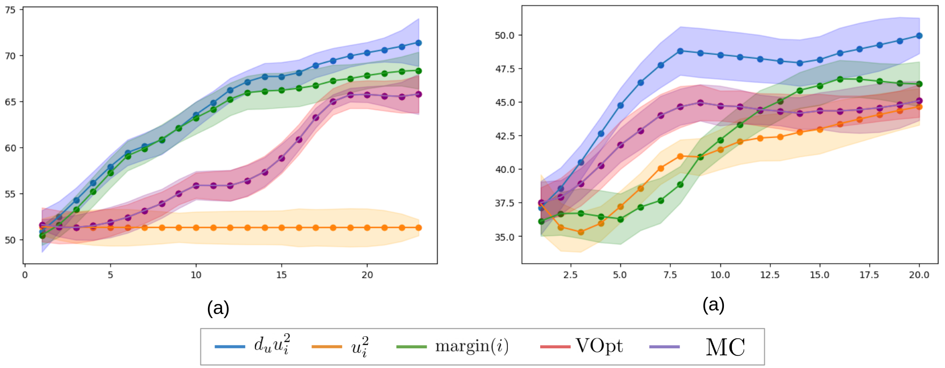
Figure 4: Performance of SSM with active learning on F-MNIST (a) and CIFAR-10 (b) Comparison between active learning methods using SSM-KL. X-axis denotes the number of vertices of the graph queries. Y-axis denotes the accuracy over 10-trials (initial labeled set). The shaded region denotes $0.5\sigma$.

We numerically evaluate our selection scheme for active learning on FashionMNIST and CIFAR-10 in Figure 4. We compare to minimum margin-based uncertainty sampling [38], VOpt [25], and Model Change (MC) [33]. Note that uncertainty sampling selects query points according to the following notion of margin: $\text{margin}(i)=\operatorname*{arg\,max}_{j}(X_{i})_{j}-\operatorname*{arg\,max}_{k\neq j}(X_{i})_{k}.$ One can interpret a smaller margin at a node as more uncertainty in the classification. We additionally note that MC and VOpt necessitate eigendecompositions of certain covariance matrices. Our score is implemented as s’(v_i) = s(v_i) - λ_t⋅margin(X), where $\lambda$ increases with $t$ via $\lambda_{t+1}=\left(1+\epsilon^{1/2k}\right)\lambda_{t}$ for some small value of $\epsilon=10^{-4}$. We show that when coupled with the proposed SSM algorithm in an iterative our active learning scheme outperforms related methods at low-label rates across all benchmarks. We also emphasize that due to certain features of SSM, the computation of $u_{i}$ is obtained for free after the first iteration.

6 Conclusion

We have proposed a novel formulation of semi supervised and active graph-based learning. Motivated by the robustness of semi-supervised Laplacian eigenmaps and spectral cuts in low label rate regimes, we introduced a formulation of Laplacian Eigenmaps with label constraints as a nonconvex Quadratically Constrained Quadratic Program. We have presented an approximate method as well as a generalization of a Sequential Subspace Method on the Stiefel Manifold. In a comprehensive numerical study on three image datasets, we have demonstrated that our approach consistently outperforms relevant methods with respect to semi-supervised accuracy in low, medium, and high label rate settings. We additionally demonstrate that selection of labeled vertices at low-label rates is critical. An active learning scheme is naturally derived from our formulation and we demonstrate it significantly improves performance, compared to competing methods. Future work includes a more rigorous analysis of the active learning score and of the problem in eq. (LABEL:eq:rescaled_f) and our algorithmic generalization of SSM—for example, conditions on $L$ and $\mathcal{U}$ that guarantee convergence to globally optimal solutions with convergence rates derived in Hager [21], Hager and Park [20], Absil et al. [2].

Overview of supplemental material. In Section A, we provide additional numerical evidence for the efficacy of our framework compared to a larger variety of methods for graph-based semi-supervised learning. We also explore the effect of the label rate at a higher resolution and compare our proposed SSM algorithm to existing open-source implementations of classic algorithms for Riemannian optimization. In Section B, we discuss an alternative perspective of our active learning score. This alternative perspective is inspired by recent literature on noise-robust sampling techniques developed in the context of graph signal processing. We derive a lower-bound on the smallest eigenvalue of $L_{\mathcal{U}}$ and demonstrate that our score is a good proxy for this bound. This implication of this bound is that our algorithm can be interpreted a greedy algorithm for degree-weighted uncertainty sampling that is robust to any underlying noise in the data or graph construction. In Section C, we provide a theoretical analysis of SSM with the goal of developing a convergence result for the algorithm. We conclude the supplemental material in Section LABEL:sec:limitations by discussing the limitations of our work and the broader societal impact of graph-based semi-supervised learning.

Appendix A Additional Results

Here, we provide additional numerical evidence for the efficacy of our framework, compared to a larger variety of graph-based semi-supervised learning algorithms.

A.1 Benchmarking graph-based semi-superivsed learning algorithms

In this section, we provide extended results on our proposed methods. First, we present average accuracy scores over additional label rates on MNIST, Fashion MNIST, and CIFAR-10. We compare our SSM approach and alignment-based approximation presented in section LABEL:sec:approx (Procrustes-SSL) against Laplace learning [56], Poisson learning [12], lazy random walks [52, 51], weighted nonlocal Laplacian (WNLL) [39], $p$-Laplace learning [16], and Laplacian Eigenmaps SSL (LE-SSL)[7]. We restrict our comparison to methods without additional cut-based refinement (e.g. PoissonMBO or KL), which we provide in the following table.

We conduct additional experiments to compare Procrustes-SSL + MBO, SSM + MBO, PoissonMBO, VolumeMBO at low ($1$, $3$, $5$) and high ($4000$) label-rates. Importantly, to conduct a fair comparison, we have augmented our proposed methods with the MBO-based refinement procedure proposed in Sec 2.4 of  Calder et al. [12] with the same set of parameters. This amounts to replacing the PoissonLearning step (line 3, Algorithm 2 of Calder et al. [12]) with either of our proposed methods (Procrustes-SSL or SSM). We show that when our method is augmented with this additional refinement step, we gain significant improvements in solution quality as well as smaller standard deviation while outperforming all MBO-based approaches. This trend notably persists through the high-label-rate regime.

Next, we evaluate the ability of our approach to retain strong predictive performance at medium and high label rates. Here, we show that Poisson Learning fails to retain superior results as compared to Laplace Learning.

Table 2: MNIST: Average accuracy over 100 trials with standard deviation in brackets. Best is bolded.

# Labels per class 1 2 3 4 5 Laplace/LP [56] 16.1 (6.2) 28.2 (10.3) 42.0 (12.4) 57.8 (12.3) 69.5 (12.2) Nearest Neighbor 55.8 (5.1) 65.0 (3.2) 68.9 (3.2) 72.1 (2.8) 74.1 (2.4) Random Walk [52] 66.4 (5.3) 76.2 (3.3) 80.0 (2.7) 82.8 (2.3) 84.5 (2.0) WNLL [39] 55.8 (15.2) 82.8 (7.6) 90.5 (3.3) 93.6 (1.5) 94.6 (1.1) p-Laplace [16] 72.3 (9.1) 86.5 (3.9) 89.7 (1.6) 90.3 (1.6) 91.9 (1.0) Poisson [12] 90.2 (4.0) 93.6 (1.6) 94.5 (1.1) 94.9 (0.8) 95.3 (0.7) LE-SSL [7] 43.1 (0.2) 87.4 (0.1) 88.2 (0.0) 90.5 (0.1) 93.7 (0.0) Procrustes-SSL 87.0 (0.1) 89.1 (0.0) 89.1 (0.0) 89.6 (0.1) 91.4 (0.0) SSM 90.6 (3.8) 94.1 (2.1) 94.7 (1.6) 95.1 (1.1) 96.3 (0.9)

Table 3: FashionMNIST: Average accuracy scores over 100 trials with standard deviation in brackets.

# Labels per class	1	2	3	4	5
Laplace/LP [56]	18.4 (7.3)	32.5 (8.2)	44.0 (8.6)	52.2 (6.2)	57.9 (6.7)
Nearest Neighbor	44.5 (4.2)	50.8 (3.5)	54.6 (3.0)	56.6 (2.5)	58.3 (2.4)
Random Walk [52]	49.0 (4.4)	55.6 (3.8)	59.4 (3.0)	61.6 (2.5)	63.4 (2.5)
WNLL [39]	44.6 (7.1)	59.1 (4.7)	64.7 (3.5)	67.4 (3.3)	70.0 (2.8)
p-Laplace [16]	54.6 (4.0)	57.4 (3.8)	65.4 (2.8)	68.0 (2.9)	68.4 (0.5)
Poisson [12]	60.8 (4.6)	66.1 (3.9)	69.6 (2.6)	71.2 (2.2)	72.4 (2.3)
LE-SSL [7]	22.0 (0.1)	51.3 (0.1)	62.0 (0.0)	65.4 (0.0)	63.2 (0.0)
Procrustes-SSL	50.1 (0.1)	55.6 (0.1)	62.0 (0.0)	63.4 (0.0)	61.3 (0.0)
SSM	61.2 (5.3)	66.4 (4.1)	70.3 (2.3)	71.6 (2.0)	73.2 (2.1)
# Labels per class	10	20	40	80	160
Laplace/LP [56]	70.6 (3.1)	76.5 (1.4)	79.2 (0.7)	80.9 (0.5)	82.3 (0.3)
Nearest Neighbor	62.9 (1.7)	66.9 (1.1)	70.0 (0.8)	72.5 (0.6)	74.7 (0.4)
Random Walk [52]	68.2 (1.6)	72.0 (1.0)	75.0 (0.7)	77.4 (0.5)	79.5 (0.3)
WNLL [39]	74.4 (1.6)	77.6 (1.1)	79.4 (0.6)	80.6 (0.4)	81.5 (0.3)
p-Laplace [16]	73.0 (0.9)	76.2 (0.8)	78.0 (0.3)	79.7 (0.5)	80.9 (0.3)
Poisson [12]	75.2 (1.5)	77.3 (1.1)	78.8 (0.7)	79.9 (0.6)	80.7 (0.5)
LE-SSL [7]	67.1 (0.0)	68.8 (0.0)	70.5 (0.0)	70.9 (0.0)	66.6 (0.0)
Procrustes-SSL	65.3 (0.0)	66.2 (0.0)	68.3 (0.0)	69.6 (0.0)	64.5 (0.0)
SSM	76.4 (1.4)	78.1 (1.3)	79.4 (0.9)	80.3 (0.7)	82.6 (0.4)

Table 4: CIFAR-10: Average accuracy scores over 100 trials with standard deviation in brackets.

# Labels per class 1 2 3 4 5 Laplace/LP [56] 10.4 (1.3) 11.0 (2.1) 11.6 (2.7) 12.9 (3.9) 14.1 (5.0) Nearest Neighbor 31.4 (4.2) 35.3 (3.9) 37.3 (2.8) 39.0 (2.6) 40.3 (2.3) Random Walk [52] 36.4 (4.9) 42.0 (4.4) 45.1 (3.3) 47.5 (2.9) 49.0 (2.6) WNLL [39] 16.6 (5.2) 26.2 (6.8) 33.2 (7.0) 39.0 (6.2) 44.0 (5.5) p-Laplace [16] 26.0 (6.7) 35.0 (5.4) 42.1 (3.1) 48.1 (2.6) 49.7 (3.8) Poisson [12] 40.7 (5.5) 46.5 (5.1) 49.9 (3.4) 52.3 (3.1) 53.8 (2.6) LE-SSL [7] 16.2 (0.1) 36.5 (0.1) 44.4 (0.1) 43.0 (0.0) 46.1 (0.0) Procrustes-SSL 36.2 (0.1) 40.6 (0.1) 44.8 (0.1) 42.9 (0.0) 45.6 (0.0) SSM 40.9 (6.1) 47.3 (5.9) 50.2 (4.3) 52.1 (4.3) 54.7 (3.4) # Labels per class 10 20 40 80 160 Laplace/LP [56] 21.8 (7.4) 38.6 (8.2) 54.8 (4.4) 62.7 (1.4) 66.6 (0.7) Nearest Neighbor 43.3 (1.7) 46.7 (1.2) 49.9 (0.8) 52.9 (0.6) 55.5 (0.5) Random Walk [52] 53.9 (1.6) 57.9 (1.1) 61.7 (0.6) 65.4 (0.5) 68.0 (0.4) WNLL [39] 54.0 (2.8) 60.3 (1.6) 64.2 (0.7) 66.6 (0.6) 68.2 (0.4) p-Laplace [16] 56.4 (1.8) 60.4 (1.2) 63.8 (0.6) 66.3 (0.6) 68.7 (0.3) Poisson [12] 58.3 (1.7) 61.5 (1.3) 63.8 (0.8) 65.6 (0.6) 67.3 (0.4) LE-SSL [7] 47.9 (0.0) 50.4 (0.0) 46.5 (0.0) 45.0 (0.0) 46.7 (0.0) Procrustes-SSL 46.1 (0.0) 50.0 (0.0) 46.9 (0.0) 45.5 (0.0) 46.9 (0.0) SSM 59.4 (2.3) 62.4 (1.7) 64.9 (1.1) 66.6 (0.4) 68.4 (0.4)

Table 5: Additional results comparing KL and MBO schemes at low and medium-high label rates.

MNIST  # Labels per class	1	3	5	4000
PoissonMBO [12]	96.5 (2.6)	97.2 (0.1)	97.2 (0.1)	97.3 (0.0)
VolumeMBO [23]	89.9 (7.3)	96.2 (1.2)	96.7 (0.6)	96.9 (0.1)
Procrustes-SSL + MBO	94.1 (0.1)	96.0 (0.0)	97.1 (0.0)	97.2 (0.0)
SSM + MBO	97.6 (0.1)	97.6 (0.1)	97.6 (0.1)	99.1 (0.0)
SSM-KL	97.6 (0.1)	97.6 (0.1)	97.6 (0.1)	99.1 (0.0)
FashionMNIST  # Labels per class	1	3	5	4000
PoissonMBO [12]	62.0 (5.7)	70.4 (2.9)	73.1 (2.7)	86.8 (0.2)
VolumeMBO [23]	54.7 (5.2)	66.1 (3.3)	70.1 (7.1)	85.5 (0.2)
Procrustes-SSL + MBO	53.6 (2.8)	60.3 (4.6)	66.5 (3.2)	70.1 (0.0)
SSM + MBO	65.3 (1.9)	71.4 (1.3)	73.2 (0.6)	93.4 (0.1)
SSM + KL	65.8 (1.1)	71.6 (1.2)	73.4 (0.3)	93.5 (0.1)
CIFAR-10  # Labels per class	1	3	5	4000
PoissonMBO [12]	41.8 (6.5)	53.5 (4.4)	57.9 (3.2)	80.1 (0.3)
VolumeMBO [23]	38.0 (7.2)	50.1 (5.7)	55.3 (3.8)	75.1 (0.2)
Procrustes-SSL + MBO	38.1 (4.7)	42.6 (3.3)	46.4 (2.9)	54.1 (0.1)
SSM + MBO	42.3 (1.5)	53.9 (2.5)	57.9 (2.1)	83.7 (0.0)
SSM-KL	43.7 (1.4)	54.1 (2.1)	58.8 (1.9)	83.9 (0.0)

Table 6: Scaling behavior as the number of labeled vertices increases beyond the low label rate regime: Average accuracy scores over 10 trials. Standard deviation across trials approaches zero for all methods. We use the publicly available implementation of Poisson Learning [11].

# Labels per class	500	1000	2000	4000
MNIST
Laplace/LP	97.8	97.9	98.1	98.3
Poisson	97.1	96.9	96.3	93.8
SSM	97.8	98.0	98.1	98.2
FashionMNIST
Laplace/LP	84.0	84.7	85.3	85.8
Poisson	82.2	78.9	74.9	58.6
SSM	84.3	84.8	85.9	86.1

A.2 Comparison with an open-source tool for Riemannian optimization

Table 7: Tool comparison: wall time per-iteration, # iterations to reach |grad| <= 10e-5 (– denotes no convergence), and accuracy using MNIST digits restricted to 0-5 with 1 label / class.

	wall time / iter	# iter to crit. point	accuracy
SSM	6.1	7	0.99
TR	145.5	10	0.94
RG	3.4	–	0.75

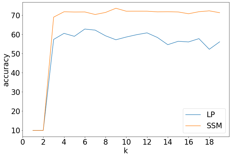
(a)

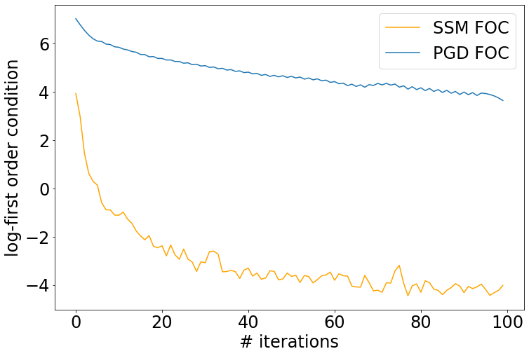
(b)

Figure 5: Robust performance of SSM on F-MNIST. (4(a)) robustness to different numbers of neighbors $k$ used to construct the graph, averaged over $10$ trials, 5 labels per-class. (4(b)) The log-first order condition, i.e. empirical rate of convergence of Projected gradient method and SSM on F-MNIST with 5 labels per-class.

Additionally, we include a comparison between the SSM component of our framework and the general first (RG) and second-order (TR) Riemannian optimization algorithms implemented in the Pymanopt package [44]. For submanifolds of Euclidean spaces, first-order methods for constrained problems that consist of iteratively taking a tangent step in the Euclidean space followed by a projection (i.e. our projected gradient method) are functionally equivalent to Riemannian Gradient methods [3, 1]. In our work, we consider the Euclidean Projection onto the Stiefel manifold given by the SVD. However, Pymanopt by default defines the retraction via the QR decomposition (although SVD-based retractions are also supported). In theory, this should yield similar convergence results in theory and practice.

We also consider the second-order trust-region method supported by Pymanopt [2]. We note that one contribution of our work is the extension of SSM, a state of the art method for large-scale trust-region subproblems to more general QCQPs. More generally, our generalization and application of SSM is motivated by its success on large scale trust-region subproblems (which our problem shares many characteristics with) - with remarkable empirical results and robust convergence guarantees, even for so-called “degenerate problems”. SSM has many advantages over typical methods for Riemannian optimization (including first and second-order trust-region methods). To summarize, we claim that our proposed SSM method + Procrustes initialization, designed specifically for the problem we propose should outperform the more general techniques implemented in Pymanopt.

We show in Fig. 4(b) that the choice of subspaces play a critical role in the rate and quality of convergence of our method (compared to first-order methods). One may also ask how our method compares to traditional second-order methods (e.g. Riemannian Trust-region). In theory, SSM employs a special set of vectors to estimate the Hessian information to update the search direction via subspace minimization. As a result, the Hessian information estimated from SSM is usually better than the Hessian estimated from CG or BFGS methods typically used for trust-region type approaches.

Figure 4(a) shows the accuracy of SSM at 5 labels per class as a function of the number of neighbors $K$ used in constructing the graph, showing that the algorithm is not significantly sensitive to this choice.

In Figure 4(b), we demonstrate the convergence behavior of SSM and the projected gradient method discussed previously by plotting the norm of the first order condition (FOC): $||LX_{t}C-BC^{1/2}-X_{t}\Lambda_{t}||$. Note that while both methods are guaranteed to monotonically reduce the objective of eq. (LABEL:eq:rescaled_f) via line search, SSM rapidly converges to a critical point, while the projected gradient method fails to converge, even after 100 iterations.

Appendix B Graph-Based Active Learning

In this section, we provide additional justification for the sampling score proposed in the main text. As mentioned in the main text, the component of score involving the eigenvector of $L_{\mathcal{U}}$ associated with the smallest eigenvalue is motivated primarily by previous work that investigates features encoded by the eigenvectors of the Laplacian of a graph with grounded vertices [14]. These features specifically facilitate efficient methods to diversely sample the graph. Additionally, our score has connections to the graph signal processing literature [24, 6] which aims to robustly recover a graph signal by sampling a sparse set of vertices. It has been demonstrated that one ideal sampling strategy that is robust to noise aims to maximize the smallest eigenvalue of the principal submatrix of the Laplacian, analogous to $L_{\mathcal{U}}$. Below, we demonstrate that our method, namely squaring the entries of $u$ and weighting by $\tilde{d}_{i}$, is directly related to one lower bound of the smallest eigenvalue of $L_{\mathcal{U}}$.

B.0.1 Lower bound estimate for eigenvalues of $L_{\mathcal{U}}$

Consider a grounded Laplacian $L_{\mathcal{U}}$ and the associated perturbation implied by labeling a vertex $E^{i}=\sum_{j\in\mathcal{U}}A_{ij}(E_{ij}+E_{ji})$, where $E_{ij}$ is an $n\times n$ matrix with $(L_{\mathcal{U}})_{ij}$ in the $ij$-th position (and, to be clear, $A_{ij}$ is a scalar). Let $u$ be one eigenvector of $L_{\mathcal{U}}$. Then, we have that the bound essentially follows from a proof of Weyl’s inequality [22]. If $G$ is connected or $|\mathcal{U}^{c}|>0$, the eigenvectors of $L_{\mathcal{U}}$ form a basis for $\mathbb{R}^{n}$. Let $v$ be a unit eigenvector of $L_{\mathcal{U}}-E^{i}$ with eigenvector decomposition (where $u^{(j)}$ is the eigenvector associated with the $j$-th eigenvalue of $L_{\mathcal{U}}$ ). v = ∑_j=1^n t_j u^(j) for some coefficients $t_{j}$ s.t. $\sum_{j}t_{j}^{2}=1$. Then the eigenvalue $\lambda^{\prime}$ of $L_{\mathcal{U}}-E^{i}$ is

$$\lambda^{\prime}=v^{\top}(L_{\mathcal{U}}-E^{i})v=\sum_{j=1}^{n}t_{j}^{2}(\lambda_{j}-\langle u^{(j)},E^{i}u^{(j)}\rangle)\geq\min_{j=1,\ldots,n}\{\lambda_{j}-\langle u^{(j)},E^{i}u^{(j)}\rangle\}$$ (17)

Thus, the maximum perturbation of the smallest eigenvalue of $L_{\mathcal{U}}-E^{i}$ is bounded below by the largest eigenvalue of $E^{i}$ (recall that $E^{i}$ has nonzero entries associated with the $i$-th column and $i$-th row of $L_{\mathcal{U}}$). Hence, to increase the eigenvalue of $L_{\mathcal{U}}$, a greedy selection implies the choice of $i$ that maximizes $-\langle u^{(j)},E^{i}u^{(j)}\rangle=2u^{(j)}_{i}\sum_{k\in\mathcal{U}}A_{ij}u^{(j)}_{k}$.

Note that when the spectral gap of $L_{\mathcal{U}}$ is large, $j$ need not be taken over $[n]$. More concretely, suppose $\lambda_{k^{\prime}+1}-\lambda_{1}>\epsilon$, where $\epsilon$ is the largest eigenvalue of $\{E^{i}\>\>:\>\>i=1,\ldots,n\}$. Note that $\lambda^{\prime}\geq\lambda$. Then,

$$\lambda^{\prime}\geq\min\{\min_{j=1,\ldots,k^{\prime}}\{\lambda_{j}-\langle u^{(j)},E^{i}u^{(j)}\rangle\},\lambda_{k^{\prime}+1}-\epsilon\}\geq\min_{j=1,\ldots,k^{\prime}}\{\lambda_{j}-\langle u^{(j)},E^{i}u^{(j)}\rangle\}$$ (18)

We highlight that the spectral gap of graph Laplacians of graphs constructed on data, particularly KNN graphs, exhibit fast growth of the eigenvalues [45, 26] and large spectral gaps. On such graphs, the low-frequency eigenvectors (eigenvectors corresponding to the smallest eigenvalues of the Laplacian) are “smooth” over the graph and the score presented in the main text is a good proxy for the above bound, i.e. $2u^{(j)}_{i}\sum_{k\in\mathcal{U}}A_{ij}u^{(j)}_{k}\approx 2\tilde{d}_{i}(u_{i})^{2}$. As we show below, using the ranking implied by just $u_{i}$ corresponds to a diversity selection strategy that iteratively selects vertices that are far from the set of labeled nodes. Intuitively, weighting this measure by $\tilde{d}_{i}$ encourages selection of vertices that are well connected. Experimentally, as shown in the main text, this also has the effect of improving results.

B.1 Spectral active learning score

For the purposes of this section, we will consider a slightly different scoring function than the one presented in the main text. Let $s(v_{i})=|u_{i}|$, where $u_{i}$ is the $i$-th component of the eigenvector of $L_{\mathcal{U}}$ corresponding to the smallest eigenvalue of $L_{\mathcal{U}}$. Note that when the graph is connected, from the Perron-Frobenius theorem [32, 22], the eigenvector associated with the smallest eigenvalue of $L_{\mathcal{U}}$ can be chosen to be elementwise nonnegative.

Proposition B.1.

Let $N_{i}$ denote the neighborhood of vertex $i$. Consider the score at vertex $v_{a}$, $s(v_{a})=|u_{i}|$. For any connected pair of vertices $v_{a}$ and $v_{b}$ such that $v_{a}\not\in N_{k}$, $v_{b}\in N_{k}$ for any $k\in\mathcal{U}^{c}$, there is a path from $v_{a}$ to $v_{b}$ such that the sequence of entries $(s(v_{a}),\ldots,s(v_{c}),\ldots s(v_{b}))$ is nonincreasing.

Proof. We will consider a vertex $v_{i}$ and its score $s(v_{i})$ when its neighborhood does not contain a labeled vertex and its score $s^{\prime}(v_{i})$ when its neighborhood does contain a labeled vertex, $v_{\ell}$. First, note that the $ith$ entry of the eigenvectors of $L_{\mathcal{U}}$ are characterized by the system d_i u_i - ∑_v_j ∈UA_iju_j = λu_i. Then, write $u_{i}=\frac{\sum_{v_{j}\in\mathcal{U}}A_{ij}u_{j}}{d_{i}-\lambda}$ and consider labeleing a single neighbor $v_{\ell}$ in the neighborhood of $v_{i}$:

$$s(v_{i})=|u_{i}|=\left|\frac{\sum_{j\in\mathcal{U}}A_{ij}u_{j}}{d_{i}-\lambda}\right| =\frac{\sum_{j\in\mathcal{U}}A_{ij}|u_{j}|}{|d_{i}-\lambda|}$$ (19)

$$\geq\frac{\sum_{j\in\mathcal{U}}A_{ij}|u_{j}|-|u_{\ell}|}{|d_{i}-\lambda|}=\left|\frac{\sum_{j\in\mathcal{U}\setminus\{u_{\ell}\}}A_{ij}u_{j}}{d_{i}-\lambda}\right|$$ (20)

$$=s^{\prime}(v_{i})$$ (21)

Naturally, the implication is that the score of a vertex decreases as its neighbors are labeled. Furthermore we have that

$$s(v_{i})=|u_{i}| =\left|\frac{\sum_{j\in\mathcal{U}}A_{ij}u_{j}}{d_{i}-\lambda}\right|\geq\frac{1}{d_{i}}\left|\sum_{j\in\mathcal{U}}A_{ij}u_{j}\right|=\frac{1}{d_{i}}\sum_{j\in\mathcal{U}}A_{ij}s(v_{j})$$ (22)

Thus, the score of a vertex $v_{i}$ is greater than the average score of its neighbors, and therefore, there must be a neighbor of $v_{i}$ with score less than $s(v_{i})$. Since each vertex has a neighbor with smaller score, starting from any vertex there is a path consisting of vertices that have decreasing scores that must finish at a vertex with neighbor in $\mathcal{U}^{c}$. ∎

Again, we emphasize that this is not necessarily true when $|u_{i}|$ is weighted by the degree $\tilde{d_{i}}$. Including this weight is intuitively motivated by the principle of connectnedness. In other words, our score selects vertices that are both distant from the set of labeled vertices, and well-connected.

Appendix C Convergence of SSM and Additional Computational Results

C.1 Preliminaries

$$\min_{X:X\in\textrm{St}(n,k)}\langle X,LXC\rangle-\langle X,BC^{1/2}\rangle$$ (23)

Quadratic minimization over the Stiefel manifold is a generalization of the well-known nonconvex quadratic over the unit ball or sphere. These problems often arise in trust region methods [42, 15]. Notably, there could exist many local solutions in 23. We will demonstrate convergence to critical points of two iterative methods: a gradient projection method and the Sequential Subspace Method proposed in this work. Furthermore, when the subspaces component to the SSM algorithm contain the span of the first $k$ nontrivial eigenvectors of $L$, we show that the quality of the stationary point is characterized by the eigenvalues of the Lagranage multipliers $\Lambda$.

First denote the the eigenvector decomposition of $L$ be given by L = [v_1, v_2, …, v_n]diag(d_1, …, d_n)[v_1, v_2, …, v_n].T

To summarize, we will show the following:

• We propose a gradient projection method to solve 23. We prove convergence with the Armijo rule in Prop. LABEL:prop:pgd_convergence.

• We analyze the proposed iterative method in the framework of SSM, constructing a sequence of subspaces to reach one approximation of local solutions, where the subspace consists of columns of $X_{t}$, $LX_{t}C-BC^{1/2}$ and eigenvectors associated with $d_{i}$, $i=1,\ldots,k$. Each sub-problem can be solved by the aforementioned gradient projection method. We demonstrate global convergence to high-quality critical points. Theoretically, when $C=I$ and the multiplicity of the first nontrivial eigenvalue is greater than or equal to $k$, a local solution is actually a global solution. However, we leave this analysis as future work.

First, we review some known results in the spherical case, i.e., $\text{St}(n,1)$. Next, we derive convergence of a projected gradient method to solutions satisfying the first order condition eq. (LABEL:eq:rescaled_f_foc). Finally, Theorem 1 states the convergence of SSM to a high-quality local solution is guaranteed.

C.1.1 Notation

We assume $k$ is a positive integer (much) less than $n$. Let $K$ denote the set $\{1,2,\ldots,k\}$. Let $I_{n,k}$ denote the sub matrix of the identity matrix $I_{n}$, consisting of the first $k$ columns. Let $O_{k}$ be the orthogonal group, i.e., $Q\in O_{k}$ if and only if $Q\in\mathbb{R}_{k,k}$ and $Q^{\top}Q=I_{k}$.

C.2 Preliminary results in the spherical case

eq. (23) is one natural generalization of the constrained problem [21, 20]

$$\min_{x}\{x^{\top}Ax-2\langle x,b\rangle:||x||=1,x\in\mathbb{R}^{n}\}$$ (24)

This problem is related to the trust region subproblem:

$$\min_{x}\{x^{\top}Ax-2\langle x,b\rangle:||x||\leq 1,x\in\mathbb{R}^{n}\}$$ (25)

The following two propositions describe the global solution of 24. See [42]. The condition 26 states that the global solution $x$ is the critical point associated with $\lambda$ bounded above by the smallest eigenvalue $d_{1}$ of $A$.

Proposition C.1 (Hager and Park [20]).

A vector $x\in\mathbb{R}^{n}$ is a global solution of 24, if and only if $||x||=1$, and

$$A-\lambda I\succcurlyeq 0,\>\>(A-\lambda I)x=b$$ (26)

holds for some $\lambda\in\mathbb{R}$

Proposition C.2 (Hager [21]).

Consider the eigenvector decomposition A = [v_1, v_2, …, v_n]diag(d_1, …, d_n)[v_1, v_2, …, v_n].T. Let $V_{1}$ be the matrix whose columns are eigenvectors of $L$ with eigenvalue $d_{1}$. Then, $x=Vc$ is a solution for a vector $c$ chosen in the following way:

• Degenerate case: suppose $V_{1}^{\top}b=0$ and $c_{\perp}:=||(A-d_{1}I)^{\dagger}b||\leq 1$ Then, $\lambda=d_{1}$ and $x=(1-c_{\perp}^{2})^{1/2}v_{1}+(A-d_{1}I)^{\dagger}b$

• Nondegenerate case: $\lambda<d_{1}$ is chosen so that $x=(A-\lambda I)^{-1}b$ with $||x||=1$.

Remark C.1 (Hager and Park [20]).

Note that $||(A-\lambda I)^{-1}b||$ decreases monotonically with respect to $\lambda\leq d_{1}$. A proper value of $\lambda$ meets the condition $||x||=1$. A tighter bound on $\lambda$ can be estimated from (d_1 - λ) ||V_1b||^2 ≤1 = ||(A - λI)^-1b||^2 ≤(d_1 - λ)^-2||b||^2 With $||V_{1}b||>0$, $\lambda$ lies in the interval $[d_{1}-||b||,d_{1}-||V_{1}b||]$

C.3 Computational results

In this section, we provide the precise computations involved in the derivation of eq. (LABEL:eq:rescaled_f) from eq. (LABEL:eq:supervised_lapeig).

C.3.1 Derivation of $B$ and $C$

Given $\mathbf{1}^{\top}X=0$ and $X^{\top}X=pI$, we have that $\mathbf{1}^{\top}X_{\mathcal{U}}=-r^{\top}$ and $X_{\mathcal{U}}^{\top}X_{\mathcal{U}}=pI-X_{l}^{\top}X_{l}=(p-\widetilde{p})I$, where $r=\mathbf{1}^{\top}X_{l}$.

Let $(\widetilde{X}_{\mathcal{U}})_{i}=(X_{\mathcal{U}})_{i}+\frac{1}{n}r$. We have the following:

1. $\mathbf{1}^{\top}\widetilde{X}_{\mathcal{U}}=0$

2. $X_{\mathcal{U}}^{\top}X_{\mathcal{U}}=\widetilde{X}_{\mathcal{U}}^{\top}\widetilde{X}_{\mathcal{U}}+\frac{1}{n}r^{\top}r$

Thus, $\widetilde{X}_{\mathcal{U}}^{\top}\widetilde{X}_{\mathcal{U}}=(p-\widetilde{p})I-\frac{1}{n}r^{\top}r$

Consider $\langle X_{0},LX_{0}\rangle=X_{\mathcal{U}}^{\top}L_{\mathcal{U}}X_{\mathcal{U}}+2X_{\mathcal{U}}^{\top}L_{\mathcal{U}l}X_{l}+X_{l}^{\top}L_{l}X_{l}$. Let $R=\frac{1}{n}\left[\begin{smallmatrix}r^{\top}\\ \vdots\\ r^{\top}\end{smallmatrix}\right]\in\mathbb{R}^{n\times k}$ We have that

$$\langle X_{0},LX_{0}\rangle =\widetilde{X}_{\mathcal{U}}^{\top}L_{\mathcal{U}}\widetilde{X}_{u}-2\widetilde{X}_{\mathcal{U}}^{\top}L_{\mathcal{U}}R$$

$$+R\top L_{\mathcal{U}}R+2\widetilde{X}_{\mathcal{U}}^{\top}L_{\mathcal{U}l}X_{l}-2R^{\top}L_{\mathcal{U}l}X_{l}+X_{l}^{\top}L_{l}X_{l}$$

$$=\widetilde{X}_{\mathcal{U}}^{\top}L_{\mathcal{U}}\widetilde{X}_{\mathcal{U}}+2\widetilde{X}_{\mathcal{U}}^{\top}(-L_{\mathcal{U}}R+L_{\mathcal{U}l}X_{l})$$

$$+R^{\top}L_{\mathcal{U}}R-2R^{\top}L_{\mathcal{U}l}X_{l}+X_{l}^{\top}L_{l}X_{l}$$

C.3.2 Pseudo-inverse of $PLP$, definiteness conditions of $X^{\top}B$, SQP Direction $Z$

Several of the algorithms we describe necessitate computation of pseudoinverse-vector products of the perturbed Laplacian $PLP$—i.e. $(PLP)^{\dagger}u$. Here, we demonstrate that the computation of $(PLP)^{\dagger}u$ is computationally comparable to computing a standard laplacian pseudoinverse-vector product, $L^{\dagger}u$, for which there exist nearly linear-time solvers [43].

Proposition C.3 (Psudo-inverse of $PL^{-1}P$).

Let $P=I-vv^{\top}$ for a unit vector $v$. Let $r_{k}=\{PL^{-1}P\}^{\dagger}u_{k-1}$. Then, the projection of $r_{k}$ is Pr_k = {PL^-1P}^†u_k-1 = (I - ¯v⊤vv⊤¯v)L^-1u_k-1, ¯v = L^-1v

Proposition C.4 (Definiteness conditions of $X^{\top}B$).

Assume $C=I$. Note the first term of $F$ satisfies the invariance $\text{tr}(X^{\top}PLPX)=\text{tr}(\widetilde{X}^{\top}PLP\widetilde{X})$, where $\widetilde{X}=XQ$ for any orthogonal $Q\in\mathbb{R}^{2\times 2}$. $X$ is a local minimizer if $X^{\top}B\succcurlyeq 0$ and symmetric.

Proof. Note that by assumption, $X$ is feasible—i.e. $X^{\top}X=I$. Consider the substitution $X\to XQ$ for some orthogonal matrix $Q$. Since $C=I$, $F(XQ)=\langle XQ,LXQ\rangle-\langle Q,X^{\top}B\rangle$.

Fix $X$. Note that the first term satisfies the invariance $\langle X,LX\rangle=\langle XQ,LXQ\rangle$. For any orthogonal $Q\in\mathbb{R}^{k\times k}$. The optimal choice of $Q$ is determined by the second term. A standard result from matrix analysis yields its minimizer [22]. Let $X^{\top}B=UDV^{\top}$ be the SVD of $X^{\top}B$. Then, $Q=U_{B}V_{B}^{\top}$ and $\langle XQ,B\rangle=\langle Q,X^{\top}B\rangle=\langle I,D\rangle=tr(D)\geq 0$. ∎

Proposition C.5 (SQP Direction of the Lagrangian Eq. eq. (LABEL:eq:rescaled_f_lagrangian)).

Assume $\Lambda$ symmetric. Let $P$ and $\Lambda C^{-1}=U\text{diag}([\lambda_{1},\ldots\lambda_{k}])U^{-1}$ be the eigenvector decomposition of $\Lambda C^{-1}$. The solution to the newton direction $Z$ of $X$ via the linearization of the FOC is given by

$$Z=OU^{\top}$$ (27)

where each column of $O$, $o_{j}=(PLP-\lambda_{j}P)^{\dagger}BC^{-1}u_{j}$.

Proof. Recall the FOC and its associated linearization with respect to descent directions of $X,\Lambda$; $(Z,\Delta)$:

$$(LZC-Z\Lambda)-X\Delta=E:=BC^{1/2}-(LXC-X\Lambda)$$

$$X^{\top}Z=0$$

Applying the projection $P^{\perp}=I-XX^{\top}$ eliminates the $X\Delta$ term: PLZ - ZΛC^-1 = PLPZ - ZUdiag([λ_1, …, λ_k])U^-1 = PEC^-1 Equivalently, PLPZU - ZUdiag([λ_1, …, λ_k]) = PEC^-1U. Let $O=ZU=[o_{1},\ldots,o_{k}]$ lie in the range of $P$. Then, PLo_j - λ_j = PEC

References

- Absil and Malick [2012] P.-A. Absil and J. Malick. Projection-like retractions on matrix manifolds. SIAM Journal on Optimization, 22(1):135–158, 2012. doi: 10.1137/100802529. URL https://doi.org/10.1137/100802529.
- Absil et al. [2007a] P.-A. Absil, C. G. Baker, and K. A. Gallivan. Trust-region methods on Riemannian manifolds. Found. Comput. Math., 7(3):303–330, July 2007a. doi: 10.1007/s10208-005-0179-9.
- Absil et al. [2007b] P.-A. Absil, R. Mahony, and R. Sepulchre. Optimization Algorithms on Matrix Manifolds. Princeton University Press, USA, 2007b. ISBN 0691132984.
- Alaoui [2016] A. E. K. Alaoui. Asymptotic behavior of -based laplacian regularization in semi-supervised learning. In Annual Conference Computational Learning Theory, 2016.
- Ando and Zhang [2006] R. Ando and T. Zhang. Learning on graph with laplacian regularization. In B. Schölkopf, J. Platt, and T. Hoffman, editors, Advances in Neural Information Processing Systems, volume 19. MIT Press, 2006. URL https://proceedings.neurips.cc/paper/2006/file/d87c68a56bc8eb803b44f25abb627786-Paper.pdf.
- Anis et al. [2015] A. Anis, A. Gadde, and A. Ortega. Efficient sampling set selection for bandlimited graph signals using graph spectral proxies. IEEE Transactions on Signal Processing, 64, 10 2015. doi: 10.1109/TSP.2016.2546233.
- Belkin and Niyogi [2002] M. Belkin and P. Niyogi. Using manifold structure for partially labelled classification. In Proceedings of the 15th International Conference on Neural Information Processing Systems, NIPS’02, page 953–960, Cambridge, MA, USA, 2002. MIT Press.
- Belkin and Niyogi [2003] M. Belkin and P. Niyogi. Laplacian eigenmaps for dimensionality reduction and data representation. Neural Computation, 15:1373–1396, 2003.
- Bertsekas [1999] D. Bertsekas. Nonlinear Programming. Athena Scientific, 1999.
- Calder [2018] J. Calder. The game theoretic p-laplacian and semi-supervised learning with few labels. Nonlinearity, 32(1):301, dec 2018. doi: 10.1088/1361-6544/aae949. URL https://dx.doi.org/10.1088/1361-6544/aae949.
- Calder [2019] J. Calder. Consistency of lipschitz learning with infinite unlabeled data and finite labeled data. SIAM Journal on Mathematics of Data Science, 1(4):780–812, 2019. doi: 10.1137/18M1199241. URL https://doi.org/10.1137/18M1199241.
- Calder et al. [2020] J. Calder, B. Cook, M. Thorpe, and D. Slepčev. Poisson learning: Graph based semi-supervised learning at very low label rates. In Proceedings of the 37th International Conference on Machine Learning, ICML’20. JMLR.org, 2020.
- Cesa-Bianchi et al. [2013] N. Cesa-Bianchi, C. Gentile, F. Vitale, and G. Zappella. Active learning on trees and graphs. CoRR, abs/1301.5112, 2013. URL http://arxiv.org/abs/1301.5112.
- Cheng et al. [2019] X. Cheng, M. Rachh, and S. Steinerberger. On the diffusion geometry of graph laplacians and applications. Applied and Computational Harmonic Analysis, 46(3):674–688, 2019. ISSN 1063-5203. doi: https://doi.org/10.1016/j.acha.2018.04.001. URL https://www.sciencedirect.com/science/article/pii/S1063520318300745.
- Conn et al. [2000] A. R. Conn, N. I. M. Gould, and P. L. Toint. Trust Region Methods. Society for Industrial and Applied Mathematics, 2000. doi: 10.1137/1.9780898719857. URL https://epubs.siam.org/doi/abs/10.1137/1.9780898719857.
- Flores et al. [2019] M. Flores, J. Calder, and G. Lerman. Analysis and algorithms for -based semi-supervised learning on graphs, 2019. URL https://arxiv.org/abs/1901.05031.
- Gerschgorin [1931] S. Gerschgorin. Uber die abgrenzung der eigenwerte einer matrix. Izvestija Akademii Nauk SSSR, Serija Matematika, 7(3):749–754, 1931.
- Golub and Van Loan [1996] G. H. Golub and C. F. Van Loan. Matrix Computations. The Johns Hopkins University Press, third edition, 1996.
- Guillory and Bilmes [2009] A. Guillory and J. A. Bilmes. Label selection on graphs. In Y. Bengio, D. Schuurmans, J. Lafferty, C. Williams, and A. Culotta, editors, Advances in Neural Information Processing Systems, volume 22. Curran Associates, Inc., 2009. URL https://proceedings.neurips.cc/paper_files/paper/2009/file/90794e3b050f815354e3e29e977a88ab-Paper.pdf.
- Hager and Park [2005] W. Hager and S. Park. Global convergence of ssm for minimizing a quadratic over a sphere. Math. Comput., 74:1413–1423, 07 2005. doi: 10.1090/S0025-5718-04-01731-4.
- Hager [2001] W. W. Hager. Minimizing a quadratic over a sphere. volume 12, 2001.
- Horn and Johnson [2013] R. A. Horn and C. R. Johnson. Matrix Analysis. Cambridge University Press, Cambridge; New York, 2nd edition, 2013. ISBN 9780521839402.
- Jacobs et al. [2018] M. Jacobs, E. Merkurjev, and S. Esedoḡlu. Auction dynamics: A volume constrained mbo scheme. Journal of Computational Physics, 354:288–310, 2018. ISSN 0021-9991. doi: https://doi.org/10.1016/j.jcp.2017.10.036. URL https://www.sciencedirect.com/science/article/pii/S0021999117308033.
- Jayawant and Ortega [2018] A. Jayawant and A. Ortega. A distance-based formulation for sampling signals on graphs. In 2018 IEEE International Conference on Acoustics, Speech and Signal Processing (ICASSP), pages 6318–6322, 2018. doi: 10.1109/ICASSP.2018.8461725.
- Ji and Han [2012] M. Ji and J. Han. A variance minimization criterion to active learning on graphs. In N. D. Lawrence and M. Girolami, editors, Proceedings of the Fifteenth International Conference on Artificial Intelligence and Statistics, volume 22 of Proceedings of Machine Learning Research, pages 556–564, La Palma, Canary Islands, 21–23 Apr 2012. PMLR. URL https://proceedings.mlr.press/v22/ji12.html.
- Keller et al. [2006] Y. Keller, R. R. Coifman, and S. Lafon. Data fusion and multicue data matching by diffusion maps. IEEE Transactions on Pattern Analysis & Machine Intelligence, 28(11):1784–1797, nov 2006. ISSN 1939-3539. doi: 10.1109/TPAMI.2006.223.
- Kernighan and Lin [1970] B. W. Kernighan and S. Lin. An efficient heuristic procedure for partitioning graphs. The Bell System Technical Journal, 49(2):291–307, 1970. doi: 10.1002/j.1538-7305.1970.tb01770.x.
- Kingma and Welling [2014] D. P. Kingma and M. Welling. Auto-Encoding Variational Bayes. In 2nd International Conference on Learning Representations, ICLR 2014, Banff, AB, Canada, April 14-16, 2014, Conference Track Proceedings, 2014.
- Krizhevsky and Hinton [2009] A. Krizhevsky and G. Hinton. Learning multiple layers of features from tiny images. (0), 2009.
- Lecun et al. [1998] Y. Lecun, L. Bottou, Y. Bengio, and P. Haffner. Gradient-based learning applied to document recognition. Proceedings of the IEEE, 86(11):2278–2324, 1998. doi: 10.1109/5.726791.
- Ma et al. [2023] J. Ma, Z. Ma, J. Chai, and Q. Mei. Partition-based active learning for graph neural networks. Transactions on Machine Learning Research, 2023. ISSN 2835-8856. URL https://openreview.net/forum?id=e0xaRylNuT. Survey Certification.
- Miekkala [1993] U. Miekkala. Graph properties for splitting with grounded laplacian matrices. BIT, 33(3):485–495, sep 1993. ISSN 0006-3835. doi: 10.1007/BF01990530. URL https://doi.org/10.1007/BF01990530.
- Miller and Bertozzi [2021] K. Miller and A. L. Bertozzi. Model-change active learning in graph-based semi-supervised learning, 2021.
- Miller and Calder [2022] K. Miller and J. Calder. Poisson reweighted laplacian uncertainty sampling for graph-based active learning, 2022.
- Miller et al. [2022] K. Miller, J. Mauro, J. Setiadi, X. Baca, Z. Shi, J. Calder, and A. L. Bertozzi. Graph-based active learning for semi-supervised classification of sar data, 2022.
- Nadler et al. [2009] B. Nadler, N. Srebro, and X. Zhou. Semi-supervised learning with the graph laplacian: The limit of infinite unlabelled data. In Proceedings of the 22nd International Conference on Neural Information Processing Systems, NIPS’09, page 1330–1338, Red Hook, NY, USA, 2009. Curran Associates Inc. ISBN 9781615679119.
- Nocedal and Wright [1999] J. Nocedal and S. J. Wright, editors. Sequential Quadratic Programming, pages 526–573. Springer New York, New York, NY, 1999. ISBN 978-0-387-22742-9. doi: 10.1007/0-387-22742-3_18. URL https://doi.org/10.1007/0-387-22742-3_18.
- Settles [2012] B. Settles. Active Learning. Synthesis Lectures on Artificial Intelligence and Machine Learning. Morgan & Claypool Publishers, 2012.
- Shi et al. [2017] Z. Shi, S. Osher, and W. Zhu. Weighted nonlocal laplacian on interpolation from sparse data. Journal of Scientific Computing, 73(2-3), 4 2017. ISSN 0885-7474. doi: 10.1007/s10915-017-0421-z. URL https://www.osti.gov/biblio/1537761.
- Silva et al. [2005] J. Silva, J. Marques, and J. a. Lemos. Selecting landmark points for sparse manifold learning. In Y. Weiss, B. Schölkopf, and J. Platt, editors, Advances in Neural Information Processing Systems, volume 18. MIT Press, 2005. URL https://proceedings.neurips.cc/paper_files/paper/2005/file/780965ae22ea6aee11935f3fb73da841-Paper.pdf.
- Slepčev and Thorpe [2019] D. Slepčev and M. Thorpe. Analysis of $p$-laplacian regularization in semisupervised learning. SIAM Journal on Mathematical Analysis, 51(3):2085–2120, 2019. doi: 10.1137/17M115222X. URL https://doi.org/10.1137/17M115222X.
- Sorensen [1982] D. C. Sorensen. Newton’s method with a model trust region modification. SIAM Journal on Numerical Analysis, 19(2):409–426, 1982. doi: 10.1137/0719026. URL https://doi.org/10.1137/0719026.
- Spielman and Teng [2014] D. A. Spielman and S.-H. Teng. Nearly linear time algorithms for preconditioning and solving symmetric, diagonally dominant linear systems. SIAM J. Matrix Anal. Appl., 35(3):835–885, jan 2014. ISSN 0895-4798.
- Townsend et al. [2016] J. Townsend, N. Koep, and S. Weichwald. Pymanopt: A python toolbox for optimization on manifolds using automatic differentiation. J. Mach. Learn. Res., 17:137:1–137:5, 2016. URL http://dblp.uni-trier.de/db/journals/jmlr/jmlr17.html#TownsendKW16.
- von Luxburg [2007] U. von Luxburg. A tutorial on spectral clustering. CoRR, abs/0711.0189, 2007. URL http://arxiv.org/abs/0711.0189.
- Wang and Mahadevan [2008] C. Wang and S. Mahadevan. Manifold alignment using procrustes analysis. In Proceedings of the 25th International Conference on Machine Learning, ICML ’08, page 1120–1127, New York, NY, USA, 2008. Association for Computing Machinery. ISBN 9781605582054. doi: 10.1145/1390156.1390297. URL https://doi.org/10.1145/1390156.1390297.
- Xiao et al. [2017] H. Xiao, K. Rasul, and R. Vollgraf. Fashion-mnist: a novel image dataset for benchmarking machine learning algorithms. ArXiv, abs/1708.07747, 2017.
- Xu et al. [2015] H. Xu, H. Zha, R.-C. Li, and M. A. Davenport. Active manifold learning via gershgorin circle guided sample selection. In AAAI Conference on Artificial Intelligence, 2015.
- Yang et al. [2006] X. Yang, H. Fu, H. Zha, and J. Barlow. Semi-supervised nonlinear dimensionality reduction. In Proceedings of the 23rd International Conference on Machine Learning, ICML ’06, page 1065–1072, New York, NY, USA, 2006. Association for Computing Machinery. ISBN 1595933832. doi: 10.1145/1143844.1143978. URL https://doi.org/10.1145/1143844.1143978.
- Zhang et al. [2023] W. Zhang, S. Pan, S. Zhou, T. Walsh, and J. C. Weiss. Fairness amidst non-iid graph data: Current achievements and future directions, 2023.
- Zhou et al. [2003] D. Zhou, O. Bousquet, T. N. Lal, J. Weston, and B. Schölkopf. Learning with local and global consistency. In NIPS, 2003.
- Zhou et al. [2004] D. Zhou, B. Schölkopf, C. Rasmussen, H. Bülthoff, and M. Giese. Learning from labeled and unlabeled data using random walks. volume 3175, 08 2004. ISBN 978-3-540-22945-2. doi: 10.1007/978-3-540-28649-3_29.
- Zhou et al. [2005] D. Zhou, J. Huang, and B. Schölkopf. Learning from labeled and unlabeled data on a directed graph. In Proceedings of the 22nd International Conference on Machine Learning, ICML ’05, page 1036–1043, New York, NY, USA, 2005. Association for Computing Machinery. ISBN 1595931805. doi: 10.1145/1102351.1102482. URL https://doi.org/10.1145/1102351.1102482.
- Zhou and Belkin [2011] X. Zhou and M. Belkin. Semi-supervised learning by higher order regularization. In G. Gordon, D. Dunson, and M. Dudík, editors, Proceedings of the Fourteenth International Conference on Artificial Intelligence and Statistics, volume 15 of Proceedings of Machine Learning Research, pages 892–900, Fort Lauderdale, FL, USA, 11–13 Apr 2011. PMLR. URL https://proceedings.mlr.press/v15/zhou11b.html.
- Zhou and Srebro [2011] X. Zhou and N. Srebro. Error analysis of laplacian eigenmaps for semi-supervised learning. In G. Gordon, D. Dunson, and M. Dudík, editors, Proceedings of the Fourteenth International Conference on Artificial Intelligence and Statistics, volume 15 of Proceedings of Machine Learning Research, pages 901–908, Fort Lauderdale, FL, USA, 11–13 Apr 2011. PMLR. URL https://proceedings.mlr.press/v15/zhou11c.html.
- Zhu et al. [2003] X. Zhu, Z. Ghahramani, and J. Lafferty. Semi-supervised learning using gaussian fields and harmonic functions. In Proceedings of the Twentieth International Conference on International Conference on Machine Learning, ICML’03, page 912–919. AAAI Press, 2003. ISBN 1577351894.
- Zhu [2005] X. J. Zhu. Semi-supervised learning literature survey. Technical report, University of Wisconsin-Madison Department of Computer Sciences, 2005.