Formally Explaining Neural Networks
within Reactive Systems

Abstract

Deep neural networks (DNNs) are increasingly being used as controllers in reactive systems. However, DNNs are highly opaque, which renders it difficult to explain and justify their actions. To mitigate this issue, there has been a surge of interest in explainable AI (XAI) techniques, capable of pinpointing the input features that caused the DNN to act as it did. Existing XAI techniques typically face two limitations: (i) they are heuristic, and do not provide formal guarantees that the explanations are correct; and (ii) they often apply to “one-shot” systems, where the DNN is invoked independently of past invocations, as opposed to reactive systems. Here, we begin bridging this gap, and propose a formal DNN-verification-based XAI technique for reasoning about multi-step, reactive systems. We suggest methods for efficiently calculating succinct explanations, by exploiting the system’s transition constraints in order to curtail the search space explored by the underlying verifier. We evaluate our approach on two popular benchmarks from the domain of automated navigation; and observe that our methods allow the efficient computation of minimal and minimum explanations, significantly outperforming the state of the art. We also demonstrate that our methods produce formal explanations that are more reliable than competing, non-verification-based XAI techniques.

1 Introduction

Deep neural networks (DNNs) [61] are used in numerous key domains, such as computer vision [58], natural language processing [26], computational biology [10], and more [23]. However, despite their tremendous success, DNNs remain “black boxes”, uninterpretable by humans. This issue is concerning, as DNNs are prone to critical errors [19, 108] and unexpected behaviors [11, 31].

DNN opacity has prompted significant research on explainable AI (XAI) techniques [85, 86, 67], aimed at explaining the decisions made by DNNs, in order to increase their trustworthiness and reliability. Modern XAI methods are useful and scalable, but they are typically heuristic; i.e., there is no provable guarantee that the produced explanation is correct [48, 20]. This hinders the applicability of these approaches to critical systems, where regulatory bars are high [72].

These limitations provide ample motivation for formally explaining DNN decisions [42, 72, 36, 20]. And indeed, the formal verification community has suggested harnessing recent developments in DNN verification [102, 73, 29, 79, 77, 39, 76, 95, 90, 32, 103, 14, 22] to produce provable explanations for DNNs [47, 17, 42]. Typically, such approaches consider a particular input to the DNN, and return a subset of its features that caused the DNN to classify the input as it did. These subsets are called abductive explanations, prime implicants or PI-explanations [93, 47, 17]. This line of work constitutes a promising step towards more reliable XAI; but so far, existing work has focused on explaining decisions of “one-shot” DNNs, such as image and tabular data classifiers [47, 17, 46], and has not addressed more complex systems.

Modern DNNs are often used as controllers within elaborate reactive systems, where a DNN’s decisions affect its future invocations. A prime example is deep reinforcement learning (DRL) [64], where DNNs learn control policies for complex systems [94, 106, 62, 68, 18, 12, 80]. Explaining the decisions of DRL agents (XRL) [82, 69, 35, 54] is an important domain within XAI; but here too, modern XRL techniques are heuristic, and do not provide formally correct explanations.

In this work, we make a first attempt at formally defining abductive explanations for multi-step decision processes. We propose novel methods for computing such explanations and supply the theoretical groundwork for justifying the soundness of these methods. Our framework is model-agnostic, and could be applied to diverse kinds of models; but here, we focus on DNNs, where producing abductive explanations is known to be quite challenging [15, 47, 17]. With DNNs, our technique allows us to reduce the number of times a network has to be unrolled, circumventing a potential exponential blow-up in runtime; and also allows us to exploit the reactive system’s transition constraints, as well as the DNN’s sensitivity to small input perturbations, to curtail the search space even further.

For evaluation purposes, we implemented our approach as a proof-of-concept tool, which is publicly available as an artifact accompanying this paper [16]. We used this tool to automatically generate explanations for two popular DRL benchmarks: a navigation system on an abstract, two-dimensional grid, and a real-world robotic navigation system. Our evaluation demonstrates that our methods significantly outperform state-of-the-art, rigorous methods for generating abductive explanations, both in terms of efficiency and in the size of the explanation generated. When comparing our approach to modern, heuristic-based XAI approaches, our explanations were found to be significantly more precise. We regard these results as strong evidence of the usefulness of applying verification in the context of XAI.

The rest of this paper is organized as follows: Sec. 2 contains background on DNNs, their verification, and their formal explainability. Sec. 3 contains our definitions for formal abductive explanations and contrastive examples for reactive systems. In Sec. 4 we propose different methods for computing such abductive explanations. We then evaluate these approaches in Sec. 5, followed by a discussion of related work in Sec. 6; and we conclude in Sec. 7.

2 Background

DNNs. Deep neural networks (DNNs) [61] are directed, layered graphs, whose nodes are referred to as neurons. They propagate data from the first (input) layer, through intermediate (hidden) layers, and finally onto an output layer. A DNN’s output is calculated by assigning values (representing input features) to the input layer, and then iteratively calculating the neurons’ values in subsequent layers. In classification, each output neuron corresponds to a class, and the input is classified as the class matching the greatest output. Fig. 1 depicts a toy DNN. The input layer has three neurons and is followed by a weighted-sum layer that calculates an affine transformation of the input values. For example, given input $V_{1}=[1,1,1]^{T}$, the second layer evaluates to $V_{2}=[7,8,11]^{T}$. This is followed by a ReLU layer, which applies the $\text{ReLU}(x)=\max(0,x)$ function to each value in the previous layer, resulting in $V_{3}=[7,8,11]^{T}$. The output layer computes the weighted sum $V_{4}=[15,-4]^{T}$. Because the first output neuron has the greatest value, $V_{1}$ is classified as the output class corresponding to that neuron.

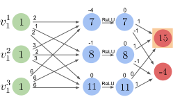
Figure 1: A toy DNN.

DNN Verification. We define a DNN verification query as a tuple $\langle P,N,Q\rangle$, where $N$ is a DNN that maps an input vector $x$ to an output vector $y=N(x)$, $P$ is a predicate over $x$, and $Q$ is a predicate over $y$ [55]. A DNN verifier needs to answer whether there exists some input $x^{\prime}$ that satisfies $P(x^{\prime})\wedge Q(N(x^{\prime}))$ (a SAT result) or not (an UNSAT result). It is common to express $P$ and $Q$ in the logic of real arithmetic [66]. The problem of verifying DNNs is known to be NP-Complete [55].

Formal Explanations for Classification DNNs. A classification problem is a tuple $\langle F,D,K,N\rangle$, where (i) $F=\{1,\ldots,m\}$is the feature set; (ii) $D=\{D_{1},D_{2},\ldots,D_{m}\}$are the domains of individual features, and the entire feature space is $\mathbb{F}=({D_{1}\times D_{2}\times\ldots\times D_{m}}$); (iii) $K=\{c_{1},c_{2},\ldots,c_{n}\}$represents the set of all classes; and (iv) $N:\mathbb{F}\to K$is the classification function, represented by a neural network. A classification instance is a pair $(v,c)$, where $v\in\mathbb{F}$, $c\in K$, and $c=N(v)$. Intuitively, this means that $N$ maps the input $v$ to class $c$.

Formally explaining the instance $(v,c)$ entails determining why $v$ is classified as $c$. An explanation (also known as an abductive explanation) is defined as a subset of features, $E\subseteq F$, such that fixing these features to their values in $v$ guarantees that the input is classified as $c$, regardless of features in $F\setminus E$. The features not part of the explanation are “free” to take on any arbitrary value, but cannot affect the classification. Formally, given an input $v=(v_{1},\ldots,v_{m})\in\mathbb{F}$ classified by the neural network to $N(v)=c$, we define an explanation as a subset of features $E\subseteq F$, such that:

$$\forall x\in\mathbb{F}.\quad\bigwedge_{i\in E}(x_{i}=v_{i})\to(N(x)=c)$$ (1)

We demonstrate formal explanations using the running example from Fig. 1. For simplicity, assume that each input can only take the values $0$ or $1$. Fig. 2 shows that the set $\{v_{1}^{1},v_{1}^{2}\}$ is an explanation for the input vector $V_{1}=[1,1,1]^{T}$: setting the first two features in $V_{1}$ to $1$ ensures that the classification is unchanged, regardless of the values the third feature takes.

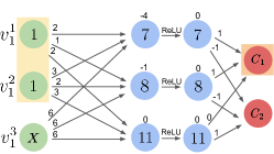
Figure 2: $\{v_{1}^{1},v_{1}^{2}\}$ is an explanation for input $V_{1}=[1,1,1]^{T}$.

A candidate explanation $E$ can be verified through a verification query $\langle P,N,Q\rangle=\langle E=v,N,Q_{\neg c}\rangle$, where $E=v$ means that all of the features in $E$ are set to their corresponding values in $v$, and $Q_{\neg c}$ implies that the classification of this query is not $c$. If this query is UNSAT, then $E$ is a valid explanation for the instance $(v,c)$.

It is straightforward to show that the set of all features is a trivial explanation. However, smaller explanations typically provide more meaningful information regarding the decision of the classifier; and we thus focus on finding minimal and minimum explanations. A minimal explanation is an explanation $E\subseteq F$ that ceases to be an explanation if any of its features are removed:

$$(\forall x\in\mathbb{F}.\quad\bigwedge_{i\in E}(x_{i}=v_{i})\to(N(x)=c))\ \wedge$$ (2)

$$(\forall j\in E.\ \exists y\in\mathbb{F}.\quad\bigwedge_{i\in E\setminus j}(y_{i}=v_{i})\wedge(N(y)\neq c))$$

A minimal explanation for our running example, $\{v_{1}^{1},v_{1}^{2}\}$, is depicted in Fig. 15 of the appendix.

A minimum explanation is a subset $E\subseteq F$ which is a minimal explanation of minimum size; i.e., there is no other minimal explanation $E^{\prime}\neq E$ such that $|E^{\prime}|<|E|$. Fig. 16 of the appendix shows that $\{v_{1}^{3}\}$ is a minimal explanation of minimal cardinality, and is hence a minimum explanation in our example.

Contrastive Examples. We define a contrastive example (also known as a contrastive explanation (CXP)) as a subset of features $C\subseteq F$, whose alteration may cause the classification of $v$ to change. More formally:

$$\exists x\in\mathbb{F}.\quad\bigwedge_{i\in F\setminus C}(x_{i}=v_{i})\wedge(N(x)\neq c)$$ (3)

A contrastive example for our running example appears in Fig. 3.

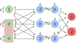
Figure 3: $\{v_{1}^{2},v_{1}^{3}\}$ is a contrastive example for $V_{1}=[1,1,1]^{T}$.

Checking whether $C$ is a contrastive example can be performed using the query $\langle P,N,Q\rangle=\langle(F\setminus C)=v,N,Q_{\neg c}\rangle$: $C$ is contrastive iff the quest is SAT. Any set containing a contrastive example is contrastive, and so we consider only contrastive examples that are minimal, i.e., which do not contain any smaller contrastive examples.

Contrastive examples have an important property: every explanation contains at least one element from every contrastive example [46, 17]. This can be used for showing that a minimum hitting set (MHS; see Sec. 2 of the appendix) of all contrastive examples is a minimum explanation [44, 84]. In addition, there exists a duality between contrastive examples and explanations [46, 50]: minimal hitting sets of all contrastive examples are minimal explanations, and minimal hitting sets of all explanations are minimal contrastive examples. This relation can be proved by reducing explanations and contrastive examples to minimal unsatisfiable sets and minimal correction sets, respectively, where this duality is known to hold [46]. Calculating an MHS is NP-hard, but can be performed in practice using modern MaxSAT or MILP solvers [63, 41]. The duality is thus useful since computing contrastive examples and calculating their MHS is often more efficient than directly computing minimum explanations [47, 46, 17].

3 K-Step Formal Explanations

A reactive system is a tuple $R=\langle S,A,I,T\rangle$, where $S$ is a set of states, $A$ is a set of actions, $I$ is a predicate over the states of $S$ that indicates initial states, and $T\subseteq S\times A\times S$ is a transition relation. In our context, a reactive system has an associated neural network $N:S\to A$. A $k$-step execution $\mathcal{E}$ of $R$ is a sequence of $k$ states $(s_{1},\ldots,s_{k})$, such that $I(s_{1})$ holds, and for all $1\leq i\leq k-1$ it holds that $T(s_{i},N(s_{i}),s_{i+1})$. We use $\mathcal{E}_{S}=(s_{1},\ldots,s_{k})$ to denote the sequence of $k$ states visited in $\mathcal{E}$, and $\mathcal{E}_{A}=(a_{1},\ldots,a_{k})$ to denote the sequence of $k$ actions selected in these states. More broadly, a reactive system can be considered as a deterministic, finite-state transducer Mealy automaton [91]. Our goal is to better understand $\mathcal{E}$, by finding abductive explanations and contrastive examples that explain why $N$ selected the actions in $\mathcal{E}_{A}$.

K-Step Abductive Explanations. Informally, we define an explanation $E$ for a $k$-step execution $\mathcal{E}$ as a subset of features of each of the visited states in $\mathcal{E}_{S}$, such that fixing these features (while freeing all other features) is sufficient for forcing the DNN to select the actions in $\mathcal{E}_{A}$. More formally, $E=(E_{1},\ldots,E_{k})$, such that $\forall x_{1},x_{2},\ldots,x_{k}\in\mathbb{F}$,

$$\big{(}\bigwedge_{i=1}^{k-1}T(x_{i},N(x_{i}),x_{i+1})\wedge\bigwedge_{i=1}^{k}\bigwedge_{j\in E_{i}}(x^{j}_{i}=s^{j}_{i})\big{)}\to\bigwedge_{i=1}^{k}N(x_{i})=a_{i}$$ (4)

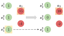
Figure 4: $(\{s^{3}\},\emptyset)$ is a (minimum) multi-step explanation for $\mathcal{E}$.

We continue with our running example. Consider the transition relation $T=\{(s,a,s^{\prime})\ |\ s^{3}=s^{\prime 3}\}$; i.e., we can transition from state $s$ to state $s^{\prime}$ provided that the third input neuron has the same value in both states, regardless of the action selected in $s$. Observe the $2$-step execution $\mathcal{E}:s_{1}=(1,1,1)\stackrel{{\scriptstyle c_{1}}}{{\to}}s_{2}=(1,0,1)\stackrel{{\scriptstyle c_{1}}}{{\to}}$, depicted in Fig. 4 (for simplicity, we omit the network’s hidden neurons), and suppose we wish to explain $\mathcal{E}_{A}=\{c_{1},c_{1}\}$. Because $\{s^{3}\}$ is an explanation for the first step, and because fixing $s^{3}_{1}$ also fixes the value of $s_{2}^{3}$, it follows that fixing $s_{1}^{3}$ is sufficient to guarantee that action $c_{1}$ is selected twice — i.e., $(\{s^{3}\},\emptyset)$ is a multi-step explanation for $\mathcal{E}$.

Given a candidate $k$-step explanation, we can check its validity by encoding Eq. 4 as a DNN verification query. This is achieved by unrolling the network $N$ for $k$ subsequent steps; i.e., by encoding a network that is $k$ times larger than $N$, with input and output vectors that are $k$ times larger than the original. We must also encode the transition relation $T$ as a set of constraints involving the input values, to mimic $k$ time-steps within a single feed-forward pass. We use $N_{[i]}$ to denote an unrolling of the neural network $N$ for $i$ steps, for $1\leq i\leq k$.

Using the unrolled network $N_{[k]}$, we encode the negation of Eq. 4 as the query $\langle P,N,Q\rangle=\langle E=\mathcal{E}_{S},N_{[k]},Q_{\neg\mathcal{E}_{A}}\rangle$, where $E=\mathcal{E}_{S}$ means that we restrict the features in each subset $E_{i}\in E$ to their corresponding values in $s_{i}$; and $Q_{\neg\mathcal{E}_{A}}$ indicates that in some step $i$, an action that is not $a_{i}$ was selected by the DNN. An UNSAT result for this query indicates that $E$ is an explanation for $\mathcal{E}$, because fixing $E$’s features to their values forces the given sequence of actions to occur.

We can naturally define a minimal $k$-step explanation as a $k$-step explanation that ceases to be a $k$-step explanation when we remove any of its features. A minimum $k$-step explanation is a minimal $k$-step explanation of the lowest possible cardinality; i.e., there does not exist a $k$-step explanation $E^{\prime}=(E^{\prime}_{1},E^{\prime}_{2},\ldots,E^{\prime}_{k})$ such that $\sum_{i=1}^{k}|E^{\prime}_{i}|<\sum_{i=1}^{k}|E_{i}|$.

K-Step Contrastive Examples. A contrastive example $C$ for an execution $\mathcal{E}$ is a subset of features whose alteration can cause the selection of an action not in $\mathcal{E}_{A}$. A $k$-step contrastive example is depicted in Fig. 5: altering the features $s_{1}^{3}$ and $s_{2}^{3}$ may cause action $c_{2}$ to be chosen instead of $c_{1}$ in the second step. Formally, $C$ is an ordered set of (possibly empty) subsets $C=(C_{1},C_{2},\ldots,C_{k})$, such that $C_{i}\subseteq F$, and for which $\exists x_{1},x_{2},\ldots,x_{k}\in\mathbb{F}$ such that

$$\begin{split}&\big{(}\bigwedge_{i=1}^{k-1}T(x_{i},N(x_{i}),x_{i+1})\big{)}\wedge\\ &\big{(}\bigwedge_{i=1}^{k}\bigwedge_{j\in F\setminus C_{i}}(x^{j}_{i}=s^{j}_{i})\big{)}\wedge\big{(}\bigvee_{i=1}^{k}N(x_{i})\neq a_{i}\big{)}\end{split}$$ (5)

Similarly to multi-step explanations, $C$ is a multi-step contrastive example iff the verification query: $\langle P,N,Q\rangle=\langle(F\setminus C_{1},F\setminus C_{2},\ldots,F\setminus C_{k})=\mathcal{E}_{S},N_{[k]},Q_{\neg\mathcal{E}_{A}}\rangle$ is SAT.

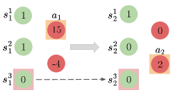
Figure 5: $(\{s^{3}\},\{s^{3}\})$ is a multi-step contrastive example for $\mathcal{E}$.

4 Computing Formal K-Step Explanations

We now propose four different methods for computing formal $k$-step explanations, focusing on minimal and minimum explanations. All four methods use an underlying DNN verifier to check candidate explanations, but differ in how they enumerate different explanation candidates until ultimately converging to an answer. We begin with the more straightforward methods.

Method 1: A Single, K-Sized Step. The first method is to encode the negation of Eq. 4 by unrolling all $k$ steps of the network, as described in Sec. 3. This transforms the problem into explaining a non-reactive, single-step system (e.g., a “one-shot” classifier). We can then use any existing abductive explanation algorithm for explaining the unrolled DNN (e.g., [47, 17, 46]).

This method is likely to produce small explanation sets but is extremely inefficient. Encoding $N_{[k]}$ results in an input space roughly $k$ times the size of any single-step encoding. Such an unrolling for our running example is depicted in Fig. 6. Due to the NP-completeness of DNN verification, this may cause an exponential growth in the verification time of each query. Since finding minimal explanations requires a linear number of queries (and for minimum explanations — a worst-case exponential number), this may cause a substantial increase in runtime.

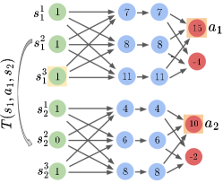
Figure 6: Finding explanations using a 2-step unrolling.

Method 2: Combining Independent, Single-Step Explanations. Here, we dismantle any $k$-step execution into $k$ individual steps. Then, we independently compute an explanation for each step, using any existing algorithm, and without taking the transition relation into account. Finally, we concatenate these explanations to form a multi-step explanation. Fixing the features of the explanation in each step ensures that the ensuing action remains the same, guaranteeing the soundness of the combined explanation.

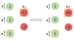
Figure 7: Explaining each step individually.

The downside of this method is that the resulting $E$ need not be minimal or minimum, even if its constituent $E_{i}$ explanations are minimal or minimum themselves; see Fig. 7. In this instance, finding a minimum explanation for each step results in the 2-step explanation $(\{s^{3}\},\{s^{3}\})$, which is not minimal — even though its components are minimum explanations for their respective steps. The reason for this phenomenon is that this method ignores the transition constraints and information flow across time-steps. This can result in larger and less meaningful explanations, as we later show in Sec. 5.

Method 3: Incremental Explanation Enumeration. We now suggest a scheme that takes into consideration the transition constraints between steps (unlike Method 2), but which encodes the verification queries for validating explanations in a more efficient manner than Method 1. The scheme relies on the following lemma:

Lemma 1.

Let $E=(E_{1},E_{2},\ldots,E_{k})$ be a $k$-step explanation for execution $\mathcal{E}$, and let $1\leq i\leq k$ such that $\forall j>i$ it holds that $E_{j}=F$. Let $E^{\prime}$ be the set obtained by removing a set of features $F^{\prime}\subseteq E_{i}$ from $E_{i}$, i.e., $E^{\prime}=(E_{1},\ldots,E_{i-1},E_{i}\setminus F^{\prime},E_{i+1},\ldots,E_{k})$. In this case, fixing the features in $E^{\prime}$ prevents any changes in the first $i-1$ actions $(a_{1},\ldots,a_{i-1})$; and if any of the last $k-i+1$ actions $(a_{i},\ldots,a_{k})$ change, then $a_{i}$ must also change.

A proof appears in Sec. 3 of the appendix. The lemma states that “breaking” an explanation $E$ of $\mathcal{E}$ at some step $i$ (by removing features from the $i$’th step), given that the features in steps $i+1,\ldots,k$ are fixed, causes $a_{i}$ to change before any other action. In this scenario, we can determine whether $E$ explains $\mathcal{E}$ using a simplified verification query: we can check whether $(E_{1},\ldots,E_{i})$ explains the first $i$ steps of $\mathcal{E}$, regardless of steps $i+1,...,k$. If so, then $a_{i}$ cannot change; and from Lemma 1, no action in $\mathcal{E}_{A}$ can change, and $(E_{1},\ldots,E_{k})$ is an explanation for $\mathcal{E}$. Otherwise, $E$ allows an action in $\mathcal{E}_{A}$ to change, and it does not explain $\mathcal{E}$. We can leverage this property to efficiently enumerate candidates as part of a search for a minimal/minimum explanation for $\mathcal{E}$, as explained next.

Finding Minimal Explanations with Method 3. A common approach for finding minimal explanations for a “one-shot” classification instance is via a greedy algorithm, which dispatches a linear number of queries to the underlying verifier [47]. Such an algorithm can start with the explanation set to be the entire feature space, and then iteratively attempt to remove features. If removing a feature allows misclassification, the algorithm keeps it as part of the explanation; otherwise, it removes the feature and continues. A pseudo-code for this approach appears in Alg. 1.

Algorithm 1 Greedy-Minimal-Explanation

Input $N$ (DNN), $F$ ($N$’s features), $v$ (values), $c$ (predicted class)

1:Explanation $\leftarrow\ F$

2:for each $f\in F$ do

3:     if verify ((Explanation$\setminus${f})=v,N,$Q_{\neg c}$) is UNSAT then

4:         Explanation $\leftarrow$ Explanation $\setminus\{f\}$      

5:return Explanation

We suggest performing a similar process for explaining $\mathcal{E}$. We start by fixing all features in all states of $\mathcal{E}$ to their values; i.e., we start with $E=(E_{1},\ldots,E_{k})$ where $E_{i}=F$ for all $i$, and then perform the following steps:

First, we iteratively remove individual features from $E_{1}$, each time checking whether the modified $E$ remains an explanation for $\mathcal{E}$. Since all features in steps $2,\ldots,k$ are fixed, it follows from Lemma 1 that checking whether the modified $E$ explains $\mathcal{E}$ is equivalent to checking whether the modified $E_{1}$ explains the selection of $a_{1}$. Thus, we perform a process that is identical to the one in the greedy Alg. 1 for finding a minimal explanation for a “one-shot” classification DNN. At the end of this phase, we are left with $E=(E_{1},\ldots,E_{k})$ where $E_{i}=F$ for all $i>1$ and $E_{1}$ was reduced by removing features from it. We keep all current features in $E$ fixed for the following steps.

Second, we begin to iteratively remove features from $E_{2}$, each time checking whether the modified $E$ still explains $\mathcal{E}$. Since the features in steps $3,\ldots,k$ are entirely fixed, it suffices (from Lemma 1) to check whether the modified $(E_{1},E_{2})$ explains the selection of the first two actions $(a_{1},a_{2})$ of $\mathcal{E}_{A}$. This is performed by checking whether

$$(\forall x_{1},x_{2}\in\mathbb{F}.\quad T(x_{1},a_{1},x_{2})\wedge\bigwedge_{j\in E_{1}}(x^{j}_{1}=s^{j}_{1})\wedge$$ (6)

$$\bigwedge_{j\in E_{2}}(x^{j}_{2}=s^{j}_{2}))\to N(x_{2})=a_{2}$$

We do not need to require that $N(x_{1})=a_{1}$ (as in Method 1) — this is guaranteed by Lemma 1. This is significant, because it exempts us from encoding the neural network twice as part of the verification query. We denote the negation of Eq. 6 for validating $(E_{1},E_{2})$ as: $\langle P,N,Q\rangle=\langle(E_{1},E_{2})=\mathcal{E}_{S_{[2]}},N,Q_{\neg a_{2}}\rangle$.

Third, we continue this iterative process for all $k$ steps of $\mathcal{E}$, and find the minimal explanation for each step separately. In step $i$, for each query we encode $i$ transitions and check whether the modified $E$ still explains the first $i$ steps of $\mathcal{E}$ (by encoding $\langle(E_{1},\ldots,E_{i})=\mathcal{E}_{S_{[i]}},N,Q_{\neg a_{i}}\rangle$), which does not require encoding the DNN $i$ times. The correctness of each step follows directly from Lemma 1.

The pseudo-code for this process appears in Alg. 2. The minimality of the resulting explanation holds because removing any feature from this explanation would allow the action in that step to change (since minimality is maintained in each step of the algorithm). An example of the first two iterations of this process on our running example appears in Fig. 8: in the first iteration, we attempt to remove features from the first step, until converging to an explanation $E_{1}$. In the second iteration, while the features in $E_{1}$ remain fixed to their values, we encode the constraints of the transition relation $T(s_{1},a_{1},s_{2})$ between the first two steps, and dispatch queries to verify candidate explanations for the second step — until converging to a minimal explanation $(E_{1},E_{2})$. In this case, $E_{2}=\emptyset$, and $(\{s^{3}\},\emptyset)$ is a valid explanation for the 2-step execution, since fixing the value of $s_{1}^{3}$ determines the value of $s_{2}^{3}$ — which forces the selection of $a_{2}$ in the second step.

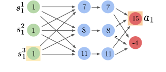
(a) First iteration

(b) Second iteration

Figure 8: Running Method 3 for finding minimal explanations, for two iterations.

We emphasize that incrementally enumerating candidate explanations for a $k$-step execution in this way is preferable to simply finding a minimal explanation by encoding verification queries that encompass all $k$-steps, à la Method 1: (i) in each iteration, we dispatch a verification query involving only a single invocation of the DNN, thus circumventing the linear growth in the network’s size — which causes an exponential worst-case increase in verification times; and (ii) in each iteration, we do not need to encode the entire set of $k$ disjuncts (from the negation of Eq. 4), since we only need to validate $a_{i}$ on the $i$’th iteration, and not all actions of $\mathcal{E}_{A}$.

Input $N$ (DNN), $F$ ($N$’s features), $\mathcal{E}$ (execution of length $k$ to explain)

Algorithm 2 Incremental-Minimal-Explanation
-Enumeration

1:Explanation $\leftarrow(E_{1},\ldots,E_{k})$ where $E_{i}=F$ for all $1\leq i\leq k$

2:for each $i\in\{1,...,k\}$ and $f\in E_{i}$ do

3:     if verify ($(E_{1},\ldots,E_{i}\setminus f)$=$\mathcal{E}_{S_{[i]}},N,Q_{\neg a_{i}}$) is UNSAT then

4:         $E_{i}\leftarrow E_{i}\setminus f$      

5:return Explanation

Finding Minimum Explanations with Method 3. We can also use our proposed enumeration to efficiently find minimum explanations, using a recursive approach. In each step $i=1,\ldots,k$, we iterate over all the possible explanations, each time considering a candidate explanation and recursively invoking the procedure for step $i+1$. In this way, we iterate over all the possible multi-step explanation candidates and can return the smallest one that we find. This process is described in Alg. 3.

Finding a minimum explanation in this manner is superior to using Method 1, for the same reasons noted before. In addition, the exponential blowup here is in the number of explanations in each step, and not in the entire number of features in each step — which is substantially smaller in many cases. Nevertheless, as the method advances through steps, it is expected to be significantly harder to iterate over all the candidate explanations. We discuss more efficient ways for finding global minimum explanations in Method 4.

Algorithm 3 Incremental-Minimum-Explanation-
Enumeration

Input $N$ (DNN), $F$ ($N$’s features), $\mathcal{E}$ (execution to explain) $\triangleright$ Global Variables

1:AllExplanations $\leftarrow$ All-Explanation-

2:Recursive-Search($\emptyset$, 1)

3:return $E\in$ AllExplanations such that $E$ is with minimum cardinality

Algorithm 4 All-Explanation-Recursive-Search

Input E (explanation), i (step number)

1:if i = k then

2:     return E

3:AllExplanations $\leftarrow\emptyset$

4:for each subset $F^{\prime}$ of $F$ do

5:     if verify ($E\cdot(F^{\prime})$=$\mathcal{E}_{S_{[i]}},N,Q_{\neg a_{i}}$) is UNSAT then

6:         Explanations $\leftarrow$ All-Explanation-

7:Recursive-Search (E $\cdot\ (F^{\prime})$, i+1)

8:         AllExplanations $\leftarrow$ AllExplanations $\cup$ Explanations      

9:return AllExplanations

Method 4: Multi-Step Contrastive Example Enumeration. As mentioned earlier, a common approach for finding minimum explanations is to find all contrastive examples, and then calculate their minimum hitting set (MHS). Because DNNs tend to be sensitive to small input perturbations [96], small contrastive examples are often easy to find, and this can expedite the process significantly [17]. When performing this procedure on a multi-step execution $\mathcal{E}$, we show that it is possible to enumerate contrastive example candidates in a more efficient manner than simply using the encoding from Method 1.

Lemma 2.

Let $\mathcal{E}$ be a $k$-step execution, and let $C=(C_{1},\ldots,C_{k})$ be a minimal contrastive example for $\mathcal{E}$; i.e., altering the features in $C$ can cause at least one action in $\mathcal{E}_{A}$ to change. Let $1\leq i\leq k$ denote the index of the first action $a_{i}$ that can be changed by features in $C$. It holds that: $C_{i}\neq\emptyset$; $C_{j}=\emptyset$ for all $j>i$; and if there exists some $l<i$ such that $C_{l}\neq\emptyset$, then all sets $\{C_{l},C_{l+1},\ldots,C_{i}\}$ are not empty.

The lemma gives rise to the following scheme. We examine some contrastive example $C^{\prime}$ of a set of subsequent steps of $\mathcal{E}$. For simplicity, we discuss the case where $C^{\prime}=(C^{\prime}_{i})$ involves only a single step $i$; but the technique generalizes to subsets of steps, as well. Such a $C^{\prime}_{i}$ can be found using a “one-shot” verification query on step $i$, without encoding the transition relation or unrolling the network. Our goal is to use $C^{\prime}$ to find many contrastive examples for $\mathcal{E}$, and use them in computing the MHS. We observe that there are three possible cases:

1. $C=(\emptyset,\ldots,\emptyset,C^{\prime}_{i},\emptyset,\ldots,\emptyset)$ already constitutes a contrastive example for $\mathcal{E}$. In this case, we say that $C^{\prime}=(C^{\prime}_{i})$ is an independent contrastive example.

2. The features in $C^{\prime}_{i}$ can cause a skew from $\mathcal{E}$ only when features from preceding steps $l,\ldots,i-1$ (for some $l<i$) are also altered. In this case, we say that $C^{\prime}$ is a dependent contrastive example, and that it depends on steps $l,\ldots,i-1$; and together, the features from all these steps form the contrastive example $C=(\emptyset,\ldots,\emptyset,C_{l},\ldots,C_{i-1},C^{\prime}_{i},\emptyset,\ldots,\emptyset)$ for $\mathcal{E}$.

3. $C^{\prime}$ is a spurious contrastive example: the first $i-1$ steps in $\mathcal{E}$, and the constraints that the transition relation imposes, prevent the features freed by $C^{\prime}_{i}$ from causing any action besides $a_{i}$ to be selected in step $i$.

Fig. 9 illustrates the three cases. The first case is identical to the one from Fig. 5, where $(\{s^{3}\})$ is a dependent contrastive example of the second step, which depends on the previous step and is part of a larger contrastive example: $(\{s^{3}\},\{s^{3}\})$. In the second case, assume that $T$ requires that $s_{3}^{1}+s_{3}^{2}\neq 1$ for any feasible transition. Thus, the assignment for $s_{2}^{3}$ which may cause the second action in the sequence to change is not reachable from the previous step, and hence $(\{s^{3}\})$ is a spurious contrastive example of the second step. In the third case, assume that $T$ allows all transitions, and hence $(\{s^{3}\})$ is an independent contrastive example for the second step; and so $(\emptyset,\{s^{3}\})$ is a contrastive example of the entire execution.

(a) Dependent

(b) Spurious

(c) Independent

Figure 9: $(\{s^{3}\})$ as a dependent, spurious and independent contrastive example.

It follows from Lemma 2 that one of these three cases must always apply. We next explain how verification can be used to classify each contrastive example of a subset of steps into one of these three categories. If $C^{\prime}$ is independent, it can be used as-is in computing the MHS; and if it is spurious, it should be ignored. In the case where $C^{\prime}$ is dependent, our goal is to find all multi-step contrastive examples that contain it, for the purpose of computing the MHS. We next describe a recursive algorithm, termed reverse incremental enumeration (RIE), that achieves this.

Reverse Incremental Enumeration. Given a contrastive example $C^{\prime}$ containing features from a set of subsequent steps of $\mathcal{E}$, we propose to classify it into one of the three categories by iteratively dispatching queries that check the reachability of $C^{\prime}$ from the previous steps of the sequence. We execute this procedure by recursively enumerating contrastive examples in previous steps. For simplicity, we assume again that $C^{\prime}=(C^{\prime}_{i})$ is a single-step contrastive example of step $i$.

1. For checking whether $C^{\prime}$ is an independent contrastive example of $\mathcal{E}$, we set $C_{i-1}=\emptyset$ and $C_{i}=C^{\prime}_{i}$, and check whether $C=(C_{i-1},C_{i})$ is a contrastive example for steps $i-1$ and $i$. This is achieved by dispatching the following query: $\exists x_{i-1},x_{i}\in\mathbb{F}$ such that:

   $$T(x_{i-1},N(x_{i-1}),x_{i})\wedge$$ (7)

   $$\big{(}\bigwedge_{l=i-1}^{i}\bigwedge_{j\in F\setminus C_{l}}(x^{j}_{l}=s^{j}_{l})\big{)}\wedge(N(x_{i})\neq a_{i})$$

   If the verifier returns SAT, $C^{\prime}_{i}$ is independent of step $i-1$, and hence independent of all steps $1,\ldots,i-1$. Hence, $C^{\prime}$ is an independent contrastive example of $\mathcal{E}$.

2. If the query from Eq. LABEL:eq:contrastive_examples_for_second_step_case_1 returns UNSAT, we now attempt to decide whether $C^{\prime}$ is dependent. We achieve this through additional verification queries, again setting $C_{i}=C^{\prime}_{i}$, but now setting $C_{i-1}$ to a non empty set of features — once for every possible set of features, separately. We again generate a query using the encoding from Eq. LABEL:eq:contrastive_examples_for_second_step_case_1, and if the verifier returns SAT it follows that $C^{\prime}$ is dependent on step $i-1$, and that $C^{\prime\prime}=(C_{i-1},C_{i})$ is a contrastive example for steps $i-1$ and $i$. We recursively continue with this enumeration process, to determine whether $C^{\prime\prime}$ is independent, dependent of step $i-2$, or a spurious contrastive example.

3. In case the previous phases determine that $C^{\prime}$ is neither independent nor part of a larger contrastive example, we conclude that it is spurious.

An example of a single reverse incremental enumeration step on a contrastive example $C^{\prime}$ in our running example is depicted in Fig. 10, and its recursive call is shown in Alg. 5 (Cxps denotes the set of all multi-step contrastive examples containing the initial $C^{\prime}$).

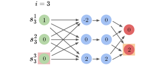
(a) First iteration

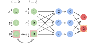
(b) Second iteration

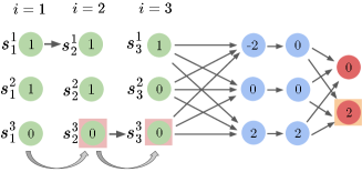
(c) Third iteration

Figure 10: An illustration of reverse incremental enumeration. We start with a single-step contrastive example, $C^{\prime}_{3}=\{s^{3}\}$ for the third step of the execution. In the second iteration, we find that $(C^{\prime}_{3})$ is dependent on the previous step, and that $(\{s^{3}\},\{s^{3}\})$ constitutes a contrastive example for steps 2 and 3. In the third iteration, $(\{s^{3}\},\{s^{3}\})$ is found to be independent of the first step, and hence $(\emptyset,\{s^{3}\},\{s^{3}\})$ is a contrastive example for $\mathcal{E}$.

Algorithm 5 Reverse Incremental Enumeration (RIE)

Input i (starting index), j (reversed index), $C^{\prime}=(C^{\prime}_{j},\ldots,C^{\prime}_{i})$

1:if j=1 then

2:     return C’ $\triangleright$ C’ is trivially independent of steps $j<1$

3:if $(\emptyset,C^{\prime}_{j},\ldots,C^{\prime}_{i})$ is a contrastive example of steps $j-1\ldots i$ then

4:     return $(C_{l}\ |\ \forall 1\leq l\leq j-1,\ C_{l}=\emptyset)\cdot C^{\prime}$ $\triangleright$ C’ is independent of step $j-1$

5:Cxps $\leftarrow\emptyset$

6:for each subset $C_{f}$ of F do

7:     if $(C_{f},C^{\prime}_{j},\ldots,C^{\prime}_{i})$ is a contrastive example of steps $j-1\ldots i$ then

8:         Cxps $\leftarrow$ Cxps $\cup$ RIE($i,j-1,C_{f}$)$\triangleright$ C’ is dependent of step $j-1$      

9:return Cxps $\triangleright$ if Cxps is empty, C’ is spurious

Using reverse incremental enumeration, we can find all multi-step contrastive examples of $\mathcal{E}$:

1. First, we find all contrastive examples for the first step of $\mathcal{E}$. This is again the same as finding contrastive examples of a “one-shot” classification problem, and can be performed efficiently [17], via Alg. 7. We first enumerate all contrastive examples of size $1$ (i.e., contrastive singletons); then all contrastive examples of size $2$ that do not contain contrastive singletons within them; and then continue this process for all $1\leq i\leq|F|$ (“skipping” all non-minimal cases).

2. Next, we search for all contrastive examples for the second step of $\mathcal{E}$, in the same manner. We perform a reverse incremental enumeration on each contrastive example found, obtaining all contrastive examples for steps 1 and 2.

3. We continue iteratively, each time visiting a new step $i$ and reversely enumerating all contrastive examples that affect steps $1,\ldots,i$. We stop when we reach the final step, $i=k$.

The full enumeration process for finding all contrastive examples of $\mathcal{E}$ is described fully in Alg. 6, which invokes Alg. 7.

Algorithm 6 Enumerate-All-Cxps

Input $N$ (DNN), $F$ ($N$’s features), $\mathcal{E}$ (execution to explain) $\triangleright$ Global Variables

1:Cxps $\leftarrow\emptyset$

2:for each $i\in\{1,...,k\}$ do

3:     CxpCandidates $\leftarrow$ Enumerate-All-Cxps-In-

4:Single-Step(i)

5:     for each Cxp $\in$ CxpCandidates do

6:         Cxps $\leftarrow$ Cxps $\cup$ RIE((Cxp), i, i)      

7:return Cxps

Algorithm 7 Enumerate-All-Cxps-In-Single-Step

Input $N$ (DNN), $F$ ($N$’s features), $\mathcal{E}$ (execution to explain), i (step number)

1:Cxps $\leftarrow\emptyset$ $\triangleright$ denotes the set of all contrastive examples

2:for each $1\leq i\leq|F|$ do

3:     for each subset $c$ of $F$ of length $i$ not containing sets from Cxps do

4:         if verify ($F\setminus c=s_{i}$,$N$,$Q_{\neg a_{i}}$) is SAT then

5:              Cxps $\leftarrow$ Cxps $\cup$ c               

6:return Cxps

We also make the following observation: we can further expedite the enumeration process by discarding sets that contain contrastive examples within them since we are specifically searching for minimal contrastive examples. For instance, in the given example in Fig. 10, if we find $(\emptyset,{s^{1}},\emptyset)$ as a contrastive example for the entire multi-step instance, we no longer need to consider sets in step $2$ that contain $s^{1}$ when iterating in reverse from step $3$ to step $2$. Our evaluation shows that this approach can significantly improve performance as the increasing number of contrastive examples found in previous steps greatly reduces the search space.

Of course, our approach’s worst-case complexity is still exponential in the number of steps, $k$, because each dependent contrastive example requires a recursive call that potentially enumerates all contrastive examples for the previous step. However, the number of recursive iterations is limited by the dependency between steps. For instance, if contrastive examples in step $i$ are only dependent on step $i-1$ and not on step $i-2$, the recursive iterations will be limited to $2$. Additionally, skipping the verification of candidates containing contrastive examples found in previous steps can also significantly reduce runtime.

5 Evaluation

Implementation and Setup. We created a proof-of-concept implementation of all aforementioned approaches and benchmarks [16]. To search for explanations, our tool [16] dispatches verification queries using a backend DNN verifier (we use Marabou [56], previously employed in additional studies [4, 7, 6, 8, 3, 5, 21, 83], although other engines may also be used). The queries encode the architecture of the DNN in question, the transition constraints between consecutive steps of the reactive system, and the candidate explanation or contrastive example being checked. Calculating the MHS, when relevant, was done using RC-2, a MaxSAT-based tool of the PySat toolkit [45].

Benchmarks. We trained DRL agents for two well-known reactive system benchmarks: GridWorld [97] and TurtleBot [99] (see Fig. 11). GridWorld involves an agent moving in a 2D grid, while TurtleBot is a real-world robotic navigation platform. These benchmarks have been extensively studied in the DRL literature. GridWorld has 8 input features per state, including agent coordinates, target coordinates, and sensor readings for obstacle detection. The agent can take $4$ possible actions: UP, DOWN, LEFT, or RIGHT. TurtleBot has $9$ input features per state, including lidar sensor readings, target distance, and target angle. The agent has $3$ possible actions: LEFT, RIGHT, or FORWARD. We trained our DRL agents with the state-of-the-art PPO algorithm [88]. Additional details appear in Sec. 5 and 6 of the appendix.

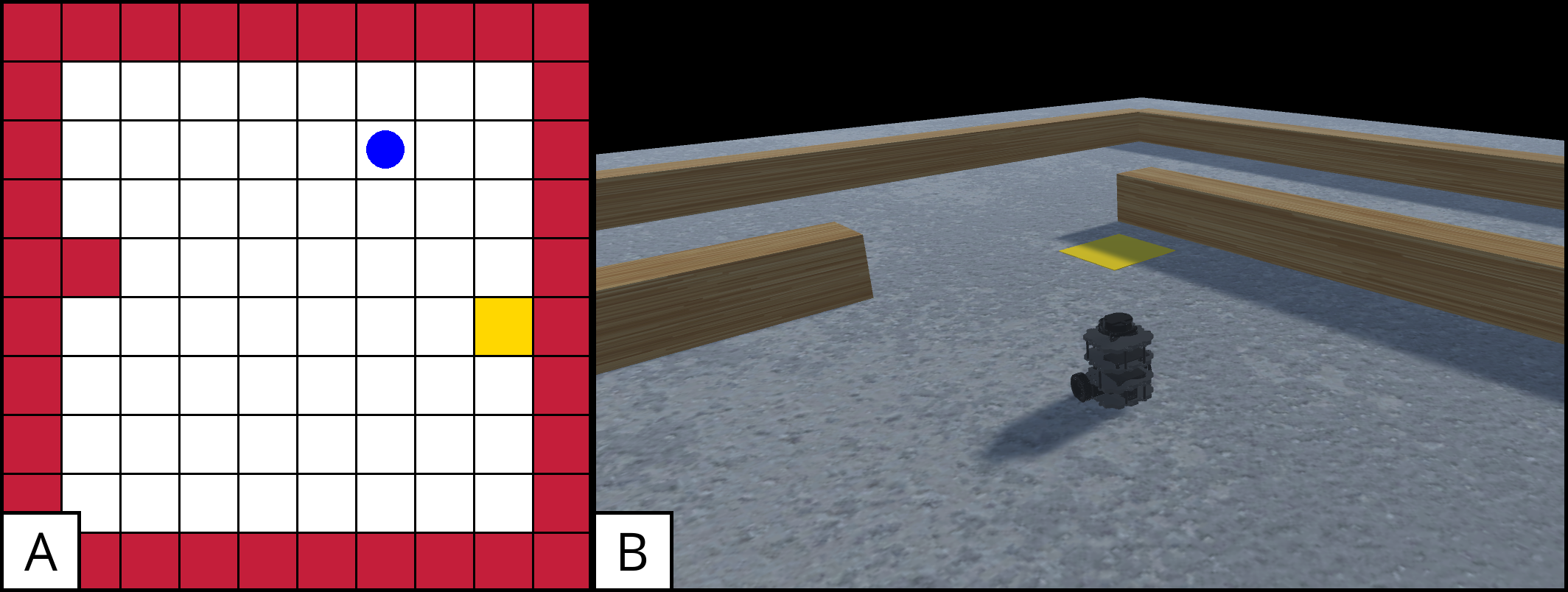
Figure 11: Benchmarks: (A) GridWorld; and (B) TurtleBot.

Generating Executions. We generated 200 unique multi-step executions of our two benchmarks: $100$ GridWorld executions (using $10$ agents, each producing $10$ unique executions of lengths $6\leq k\leq 14$), and $100$ TurtleBot executions (using $100$ agents, each producing a single execution of length $6\leq k\leq 8$). Next, from each $k$-step execution, we generated $k$ unique sub-executions, each representing the first $i$ steps of the original execution ($1\leq i\leq k$). This resulted in a total of $931$ GridWorld executions and $647$ Turtlebot executions. We used these executions to assess the different methods for finding minimal and minimum explanations. Each experiment ran with a timeout value of $3\cdot i$ hours, where $i$ is the execution’s length.

Experiments. We begin by comparing the performance of the four methods discussed in Sec. 4: (i) encoding the entire network as a “one-shot” query; (ii) computing individual explanations for each step; (iii) incrementally enumerating explanations; and (iv) reversely enumerating contrastive examples and calculating their MHS. We note that we use Methods 1–3 to generate both minimal and minimum explanations, whereas Method $4$ is only used to generate minimum explanations. To generate minimum explanations using the “one-shot” encodings of Methods $1$ and $2$, we use the state-of-the-art approach of Ignatiev et al. [47]. We use two common criteria for comparison [47, 17, 46]: the size of the generated explanations (small explanations tend to be more meaningful), and the overall runtime and timeout ratios.

Results. Results for the GridWorld benchmark are presented in Table 1. These results clearly indicate that Method 2 (generating explanations in independent steps) was significantly faster in all experiments, but generated drastically larger explanations — about two times larger when searching for a minimal explanation, and about five times larger for a minimum explanation, on average. This is not surprising; as noted earlier, the explanations produced by such an approach do not take the transition constraints into account, and hence, may be quite large. In addition, we note again that this approach does not guarantee the minimality of the combined explanation, even when combining minimal/minimum explanations for each step. The corresponding results for TurtleBot appear in Sec. 7 of the appendix, and also demonstrate similar outcomes.

Table 1: GridWorld: columns from left to right: experiment type, method name (and number), time and size of returned explanation (out of experiments that terminated), and the percent of solved instances (the rest timed out). The bold highlighting indicates the method that generated the explanation with the optimal size.

setting	experiment	time (s)	size			solved (%)
		avg.	min	avg.	max
minimal (local)	one-shot (1)	304	5	33	112	98
	independent (2)	1	5	34	97	99.9
	incremental (3)	1	5	18	78	99.7
minimum (global)	one-shot (1)	405	5	14	32	29.8
	independent (2)	4	5	35	98	98.3
	incremental (3)	1,396	5	7	9	17.9
	reversed (4)	39	5	7	16	99.7

When comparing the three approaches that can guarantee minimal explanations, the incremental enumeration approach (Method 3) is clearly more efficient than the “one-shot” scheme (running for about $1$ second compared to above $5$ minutes, on average, across all solved instances), as depicted in Fig. 12. For the minimum explanation comparison, the results show that the reversed-enumeration-based strategy (Method 4) ran significantly faster than all other methods that can find guaranteed minimum explanations: on average, it ran for $39$ seconds, while the other methods ran for more than $6$ and $23$ minutes. In addition, out of all methods guaranteed to produce a minimum explanation, experiments that ran with the “reversed” strategy hit significantly fewer timeouts. The “reversed” strategy outperforms the competing methods significantly, on both benchmarks (see Fig. 13).

Next, we analyzed the strategies at a higher resolution — focusing on a step-wise level comparison, i.e., on analyzing how the length of the execution affected runtime. The results (see Figs. 17- 20 of the appendix) demonstrate the drastic performance gain of our “reversed” strategy as $k$ increases: this strategy can efficiently find explanations for longer executions, while the competing “one-shot” strategy fails. This again is not surprising: when dealing with large numbers of steps, the transition function, the unrolling of the network, and the underlying enumeration scheme become more taxing on the underlying verifier. A full analysis of both benchmarks, and all explanation types, appears in Sec. 7 of the appendix.

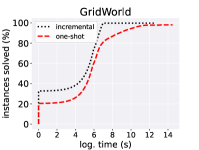
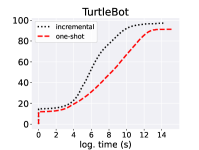
Figure 12: Minimal explanation: number of solved instances depending on (accumulative) time, for the methods that guarantee minimality.

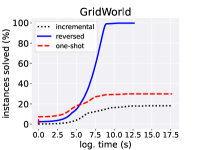
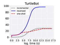
Figure 13: Minimum explanation: number of solved instances depending on (accumulative) time, for the methods that guarantee minimality.

Explanation Example. We provide a visual example of an instance from our GridWorld experiment identified as a minimum explanation. The results (depicted in Fig. 14) include a minimum explanation for an execution of $8$ steps. They show the following meaningful insight: fixing part of the agent’s location sensors at the initial step, and a single sensor in the sixth step, is sufficient for forcing the agent to move along the original path, regardless of any other sensor reading.

Figure 14: GridWorld: a $5$-sized explanation for an $8$-step execution. The steps are numbered (in blue circles), the target is the yellow square, and the obstacles are depicted in red.

Comparison to Heuristic XAI Methods. We also compared our results to popular, non-verification-based, heuristic XAI methods. Although these methods proved scalable, they often returned unsound explanations when compared to our approach. For additional details, see Section 8 of the appendix.

6 Related Work

This work joins recent efforts on utilizing formal verification to explain the decisions of ML models [47, 93, 92, 17, 104, 28, 59]. Prior studies primarily focused on formally explaining classification over various domains [47, 17, 104, 47, 48, 59] or specific model types [38, 71, 51, 43, 49]. while others explored alternative ways of defining explanations over classification tasks [104, 59, 52, 101, 9, 81, 74, 37].

Methods closer to our own have focused on formally explaining DNNs [47, 17, 104, 59, 40], where the problem is known to be complex [65, 47]. This work relies on the rapid development of DNN verification [55, 105, 30, 13, 57, 14, 1, 33]. There has also been ample work on heuristic XAI [85, 86, 67, 34, 89], including approaches for explaining the decisions of reinforcement-learning-based reactive systems (XRL) [82, 69, 35, 54]. However, these methods do not provide formal guarantees.

7 Conclusion

Although DNNs are used extensively within reactive systems, they remain “black-box” models, uninterpretable to humans. We seek to mitigate this concern by producing formal explanations for executions of reactive systems. As far as we are aware, we are the first to provide a formal basis of explanations in this context, and to suggest methods for efficiently producing such explanations — significantly outperforming the competing approaches. We also note that our approach is agnostic to the type of reactive system, and can be generalized beyond DRL systems, to any k-step reactive DNN system (including RNNs, LSTMs, GRUs, etc.). Moving forward, a main extension could be scaling our method, beyond the simple DRLs evaluated here, to larger systems of higher complexity. Another interesting extension could include evaluating the attribution of the hidden-layer features, rather than just the input features.

Acknowledgments. The work of Bassan, Amir, Refaeli, and Katz was partially supported by the Israel Science Foundation (grant number 683/18). The work of Amir was supported by a scholarship from the Clore Israel Foundation. The work of Corsi was partially supported by the “Dipartimenti di Eccellenza 2018-2022” project, funded by the Italian Ministry of Education, Universities, and Research (MIUR).

Appendix

1 Examples of Minimal and Minimum Explanations

We present figures depicting a minimal explanation, and a minimum explanation, for the toy DNN (depicted in Fig. 1), and the input $V_{1}=[1,1,1]^{T}$.

Figure 15: $\{v_{1}^{1},v_{1}^{2}\}$ is a minimal explanation for input $V_{1}=[1,1,1]^{T}$.

Figure 16: $\{v_{1}^{3}\}$ is a minimum explanation for input $V_{1}=[1,1,1]^{T}$.

2 Minimum Hitting Set (MHS)

Given a collection $\mathbb{S}$ of sets from a universe U, a hitting set $h$ for $\mathbb{S}$ is a set such that $\forall S\in\mathbb{S},h\cap S\neq\emptyset$. A hitting set $h$ is said to be minimal if none of its subsets is a hitting set, and minimum if it has the smallest possible cardinality among all existing hitting sets.

3 Additional Proofs

We present the full proofs for the three lemmas mentioned in this work.

Lemma 1.

Let $E=\{E_{1},E_{2},\ldots E_{k}\}$ be a $k$-step explanation for execution $\mathcal{E}$, and let $1\leq i\leq k$. Let $E^{\prime}$ be the set obtained by removing a set of features $F^{\prime}\subseteq E_{i}$ from $E_{i}$, i.e., $E^{\prime}=(E_{1},\ldots,E_{i-1},E_{i}\setminus F^{\prime},E_{i+1},\ldots,E_{k})$. In this case, fixing the features in $E^{\prime}$ prevents the first $i-1$ actions, $(a_{1},a_{2},\ldots a_{i-1})$, from changing.

Proof.

After removing $F^{\prime}$ from $E$, when validating if $E^{\prime}$ is an explanation for $\mathcal{E}$, then all features in $(E_{1},\ldots,E_{i-1})$ are still fixed to their corresponding values. Assume by contradiction that one of the actions $(a_{1},a_{2},\ldots a_{i-1})$ changed, then $(E_{1},\ldots,E_{i-1})$ is not an explanation for the first $i-1$ steps of $\mathcal{E}$, contradicting the assumption. Hence, actions $(a_{1},a_{2},\ldots a_{i-1})$ were selected. ∎

Lemma 2.

Let $E=(E_{1},E_{2},\ldots,E_{k})$ be a $k$-step explanation for execution $\mathcal{E}$, and let $1\leq i\leq k$ such that $\forall j>i$ it holds that $E_{j}=F$. Let $E^{\prime}$ be the set obtained by removing a set of features $F^{\prime}\subseteq E_{i}$ from $E_{i}$, i.e., $E^{\prime}=(E_{1},\ldots,E_{i-1},E_{i}\setminus F^{\prime},E_{i+1},\ldots,E_{k})$. In this case, fixing the features in $E^{\prime}$ prevents any changes in the first $i-1$ actions $(a_{1},\ldots,a_{i-1})$, and if at least one of the last $k-i+1$ actions $(a_{i},\ldots,a_{k})$ changed, then $a_{i}$ must have changed.

Proof.

When fixing the features of $E^{\prime}$ to their corresponding values, it holds from Lemma 1 that actions $(a_{1},\ldots,a_{i-1})$ were selected. Assume by contradiction that some $a_{j}$ such that $j>i$ changed, and that $a_{i}$ did not. If $a_{i}$ did not change, hence $(E_{1},\ldots,E_{i})$ is an explanation for the first $i$ steps of $\mathcal{E}$. More formally, $\forall x_{1},x_{2},\ldots,x_{i}\in\mathbb{F}$:

$$\big{(}\bigwedge_{l=1}^{i}T(x_{l},N(x_{l}),x_{l+1})\wedge\bigwedge_{l=1}^{i}\bigwedge_{r\in E_{l}}(x^{r}_{l}=s^{r}_{l})\big{)}\to\bigwedge_{l=1}^{i}N(x_{l})=a_{l}$$ (8)

Since we know that $a_{i}$ occurred then we know that $T(x_{i},N(x_{i}),x_{i+1})$ holds, and since all features in steps $i+1,\ldots,k$ are fixed to their original values then fixing them clearly determines $N(x_{l})=a_{l}$ for all $l\geq i$ and that the transitions $T(x_{l},N(x_{l}),x_{l+1})$ also hold. Overall we get that $\forall x_{1},x_{2},\ldots,x_{k}\in\mathbb{F}$:

$$\big{(}\bigwedge_{l=1}^{k}T(x_{l},N(x_{l}),x_{l+1})\wedge\bigwedge_{l=1}^{k}\bigwedge_{r\in E_{l}}(x^{r}_{l}=s^{r}_{l})\big{)}\to\bigwedge_{l=1}^{k}N(x_{l})=a_{l}$$ (9)

meaning that $(E_{1},\ldots,E_{k})$ is an explanation for $\mathcal{E}$. Hence, it is not possible for $a_{j}$ to be altered, contradicting the assumption. ∎

Lemma 3.

Let $\mathcal{E}$ be a $k$-step execution, and let $C=\{C_{1},\ldots,C_{k}\}$ be a minimal contrastive example for $\mathcal{E}$; i.e., altering the features in $C$ can cause at least one action in $\mathcal{E}_{A}$ to change. Let $1\leq i\leq k$ denote the index of the first action $a_{i}$ that can be changed by features in $C$. It holds that: $C_{i}\neq\emptyset$; $C_{j}=\emptyset$ for all $j>i$; and if there exists some $l<i$ such that $C_{l}\neq\emptyset$, then all sets $\{C_{l},C_{l+1},\ldots,C_{i}\}$ are not empty.

Proof.

Since $a_{i}$ denotes the first action that can be potentially changed by altering the values of $C$, then all actions $(a_{1},...,a_{i-1})$ were selected, and thus $(F\setminus C_{1},\ldots,F\setminus C_{i-1})$ is an explanation for the first $i-1$ steps of $\mathcal{E}$. It also holds that $(C_{1},\ldots,C_{i})$ is a contrastive example for the first $i$ steps of $\mathcal{E}$, since altering its values can cause $a_{i}$ to change.

First, assume by contradiction that there exists some $C_{j}\neq\emptyset$ for some $j>i$. Since $(C_{1},\ldots,C_{i})$ is a contrastive example for the first $i$ steps of $\mathcal{E}$, then there exists some contrastive example $C^{\prime}=(C_{1},\ldots,C_{i},\emptyset\ldots,\emptyset)$ for $\mathcal{E}$. Since $|C^{\prime}|<|C|$, it thus holds that $C=(C_{1},\ldots,C_{k})$ is not minimal. Hence, $C_{j}=\emptyset$ for all $j>i$.

Second, assume by contradiction that $C_{i}=\emptyset$. Since we proved that $C_{j}=\emptyset$ for all $j>i$ then $C=\{C_{1},\ldots,C_{i-1},\emptyset,\ldots,\emptyset\}$. Let there be some $E=\{E_{1},\ldots,E_{k}\}$ such that for all $1\leq i\leq k$ it holds that $E_{i}=F\setminus C_{i}$. Since $C_{j}=\emptyset$ for all $j>i$ then it holds that for all $j>i$, $E_{j}=F$. Since we also know that $(F\setminus C_{1},\ldots,F\setminus C_{i-1})$ is an explanation for the first $i-1$ steps then it follows from Lemma 2 that when fixing the values of $E$, and allowing the values of $C$ to alternate freely, then it holds that if some $a_{l}$ changed such that $l>i-1$ then $a_{i-1}$ must also change. But we know that $a_{i}$ was changed and that $a_{i-1}$ was selected, contradicting the assumption. Hence, $C_{i}\neq\emptyset$.

Third, assume that there exists some $l<i$ such that $C_{l}\neq\emptyset$. Assume by contradiction that not all sets $\{C_{l},C_{l+1},\ldots,C_{i}\}$ are not empty, i.e, there exists some $C_{d}=\emptyset$ such that $l\leq d\leq i$. Since $C_{l}\neq\emptyset$ and $C_{i}\neq\emptyset$, it follows that $l<d<i$. Let there be some $E=(F\setminus C_{1},\ldots,F\setminus C_{k})$. Since $(F\setminus C_{1},\ldots,F\setminus C_{i-1})$ is an explanation for the first $i-1$ steps of $\mathcal{E}$, and $d\leq i-1$, then $(F\setminus C_{1},\ldots,F\setminus C_{d})$ is an explanation for the first $d$ steps. Thus, fixing the features in $E$ to their corresponding values (and allowing the features in $C$ to alternate arbitrarily) forces the first $d$ actions to occur. Since $C_{d}=\emptyset$ then $E_{d}=F$, meaning it is entirely fixed, and thus alternating the values of any one of the sets: $(C_{1},\ldots,C_{d-1})$ clearly cannot affect any of the actions $(a_{d},\ldots,a_{k})$. Particularly, since $l<d$, alternating the values of $C_{l}$ cannot cause actions $(a_{d},\ldots,a_{k})$ to change. Hence, there exists some $C^{\prime}=(C_{1},\ldots,C_{l-1},\emptyset,C_{l+1},\ldots,C_{k})$, which is also a contrastive example for $\mathcal{E}$. $|C^{\prime}|<|C|$, and hence, it again holds that $C$ is not minimal, contradicting the assumption.

∎

4 Deep Reinforcment Learning

Deep reinforcement learning (DRL) [64] is a specific paradigm in machine learning that seeks to learn models that will be deployed within complex and reactive environments. In DRL, a DNN agent is trained to learn a policy $\pi$, that maps an observed state $s$ to an action $a$. The policy can be either deterministic or stochastic, depending on the chosen setting and the various learning algorithms. During training, a reward $r_{t}$ is assigned to the agent at each time-step $t\in{0,1,2...}$, based on the action $a_{t}$ performed at time-step $t$. Various DRL training algorithms leverage the reward differently [97, 98, 88]. However, the final goal is to find the optimal policy $\pi$ that maximizes the expected cumulative discounted reward. In recent years, DRL-trained agents have demonstrated promising results in a large variety of tasks, from game playing [75] to robotic navigation [70], and more. Since DRL-based agents are deployed within reactive systems — various DRL verification tools unroll the DRL agent for a finite number of steps, before verifying the property of interest among these encoded time-steps [6, 27].

5 Training the DRL Models

In the following section, we go into further detail about the hyperparameters applied during training and the specific implementation methods used. The training process was executed using the BasicRL baselines.

General parameters and algorithmic implementation. For the training, we exploited the Proximal Policy Optimization (PPO) algorithm based on an Actor-Critic structure. The strategy for the critic’s training is a pure Monte Carlo approach without temporal difference rollouts. The actor network is updated periodically after a sequence of data collection episodes. The actor update rule follows the original implementation of [88]. For reproducibility, we set the same random seed for the Random, NumPy and TensorFlow Python modules.

Parameters for the GridWorld environment.

• memory limit: None

• gamma: 0.99

• trajectory update frequency: 10

• trajectory reduction strategy: sum

• actor-network size: 2 layers of 8 neurons each

• critic batch size: 128

• critic epochs: 60

• critic-network size: same as actor

• PPO clip: 0.2

• reward: $+1$ for reaching the target and $0$ otherwise

• random seeds: $[207,700]$

Parameters for the TurtleBot environment.

• memory limit: None

• gamma: 0.99

• trajectory update frequency: 10

• trajectory reduction strategy: sum

• actor-network size: 2 layers of 32 neurons each

• critic batch size: 128

• critic epochs: 60

• critic-network size: same as actor

• PPO clip: 0.2

• reward: same as [3]

• random seeds: $[49,80,99,211,233]$

All original agents can be found in our publicly-available artifact accompanying this paper [16].

6 Property Constraints & Transition Functions

Next, we provide details regarding the transition functions of both benchmarks. This, in turn, defined the queries which we dispatched to our backend verifier (we used Marabou [56], which was previously used in additional settings [7, 8, 4, 5, 21, 24, 83, 78, 60, 53]). We also note that in order to speed verification for the GridWorld queries, we also configured Marabou to incorporate the Gurobi LP solver.

6.1 GirdWorld

Inputs. The DRL-based agent has $8$ inputs in total. These represent the location of the agent and the target, as well as discrete sensor reading values indicating the closest obstacle in each direction. More specifically, the DRL-based agent receives:

• $2$ inputs ($x_{0}$,$x_{1}$) representing the discrete 2D coordinates of the agent.

• $2$ inputs ($x_{2}$,$x_{3}$) representing the discrete 2D coordinates of the target.

• $4$ input sensor readings ($x_{4}$,$x_{5}$,$x_{6}$,$x_{7}$) indicating if the agent senses an obstacle in one of four directions: UP, DOWN, LEFT, or RIGHT.

Outputs. The agent has $4$ outputs, each representing one of four possible actions to move in the current step: UP, DOWN, LEFT, or RIGHT.

Trivial Bounds.

• all the DNN’s inputs are normalized to the range $[0,1]$.

• the location inputs (i.e., $x_{i}$ for $i\in[0,1,2,3]$) have a value $v\in\{0.1,0.2,\ldots,1\}$. Each of these values represents a separate location on one of the axes of the $10X10$ grid.

• the sensor reading inputs (i.e., $x_{i}$ for $i\in[4,5,6,7]$) have a value $v\in\{0,\frac{1}{2},1\}$ indicating if, and how far, an obstacle is in the relevant direction. For example, if for the RIGHT input sensor reading, the value is $1$, then if the agent will decide to move RIGHT, it will collide; if the sensor reading value is $\frac{1}{2}$, then there is an obstacle two steps to the right (and hence two subsequent RIGHT actions will result in a collision). If the sensor reading is zero, then the closest obstacle on the right direction is at least three steps away from the current state.

Transitions. We will elaborate on the transitions for moving in a given direction $d\in\{\texttt{LEFT},\texttt{RIGHT},\texttt{UP},\texttt{DOWN}\}$ (the transition function is symmetric along all axes and so it encodes all possible transitions). For a movement in direction $d$ at some time-step $t$:

• agent’s location on the axis matching the direction d: $x_{d-axis}^{t}=x_{d-axis}^{t+1}\pm 0.1$ (the sign depends on d)

• agent’s location on the axis orthogonal to the direction d: $x_{orthogonal-d-axis}^{t}=x_{orthogonal-d-axis}^{t+1}$

• target’s location does not change: $x_{2}^{t}=x_{2}^{t+1}$, $x_{3}^{t}=x_{3}^{t+1}$

• obstacle sensor reading in the direction of movement:
  $x_{sensor-d}^{t}\leq x_{sensor-d}^{t+1}\leq x_{sensor-d}^{t}+\frac{1}{2}$

• obstacle sensor reading in the direction of movement:
  $x_{sensor-d}^{t}+x_{sensor-d}^{t+1}\in\{0,\frac{1}{2},1\}$

• obstacle sensor reading in the opposite direction of movement:
  $x_{sensor-opposite-d}^{t}-\frac{1}{2}\leq x_{sensor-opposite-d}^{t+1}\leq x_{sensor-opposite-d}^{t}$

• obstacle sensor reading in the opposite direction of movement:
  $x_{sensor-opposite-d}^{t}+x_{sensor-opposite-d}^{t+1}\in\{0,\frac{1}{2},1\}$

6.2 TurtleBot

Inputs. The DRL-based agent has $9$ inputs in total:

• $7$ inputs: ($x_{0},x_{1},\ldots,x_{6}$) representing the lidar sensors. Each set of subsequent inputs represents lidar sensors aimed at $30\degree$ between one another.

• $1$ input ($x_{7}$) indicating the angle between the agent and the target.

• $1$ input ($x_{8}$) indicating the distance between the agent and the target.

Outputs. The agent also has $3$ outputs: $<y_{0},y_{1},y_{2}>$, that correspond to the actions $<\texttt{FORWARD},\texttt{LEFT},\texttt{RIGHT}>$.

Trivial Bounds. all the DNN’s inputs are normalized to the range $[0,1]$.

Transitions. For simplicity, we focused on properties in which each one of the steps (except, perhaps, the last) is either RIGHT or LEFT (see [3]):

• RIGHT action (output at time-step $t$):

  • bounds: $x_{i}^{t}\in[0.2,1]\text{ for }i=[0,1,2,3,4,5,6,8]\text{ and }\land x_{7}^{t}\in[0,1]$

  • lidar “sliding window”: $\text{ for }i=[1,2,3,4,5,6]$: $x_{i}^{t}=x_{i-1}^{t+1}$

  • turn $30\degree$ to the right: $x_{7}^{t+1}=x_{7}^{t}-\frac{1}{12}$

  • distance to target does not change: $x_{8}^{t}=x_{8}^{t+1}$

• LEFT action (output at time-step $t$):

  • bounds: $x_{i}^{t}\in[0.2,1]\text{ for }i=[0,1,2,3,4,5,6,8]\text{ and }\land x_{7}^{t}\in[0,1]$

  • lidar “sliding window”: $\text{ for }i=[1,2,3,4,5,6]$: $x_{i-1}^{t}=x_{i}^{t+1}$

  • turn $30\degree$ to the left: $x_{7}^{t+1}=x_{7}^{t}+\frac{1}{12}$

  • distance to target does not change: $x_{8}^{t}=x_{8}^{t+1}$

7 Supplementary Results

TurtleBot Results. Table. 2 presents the full results of the four aforementioned approaches on the TurtleBot benchmark.

Table 2: TurtleBot: columns from left to right: experiment type, method name, method number, time and size of the returned explanation (out of experiments that terminated), the percent of solved instances (the rest timed out), and a column indicating whether the explanation is guaranteed to be minimal. The bold highlighting indicates the method that generated the explanation with the optimal size.

setting	experiment	M	time (s)	size			solved (%)	guaranteed minimality
			avg.	min	avg.	max
minimal (local)	one-shot	1	1,084	2	6	12	91.2	✔
	independent	2	1	4	24	54	100	✘
	incremental	3	764	2	6	10	97.1	✔
minimum (global)	one-shot	1	2,228	2	6	10	27.1	✔
	independent	2	77	2	17	37	100	✘
	incremental	3	637	2	6	11	28.8	✔
	reversed	4	267	2	5	10	96.8	✔

Full Evaluation by Execution Size. We present here the full analysis of the results, evaluated under different execution sizes (number of steps) both for the minimal and minimum explanation settings, for the two benchmarks. Fig. 17 presents the results for GridWorld under the minimal explanation setting, and Fig. 18 for the minimum explanation setting. Fig. 19 presents the results for TurtleBot under the minimal explanation setting, and Fig. 20 for the minimum explanation setting

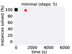
Figure 17: GridWorld: solved instances of minimal explanation search, by (accumulative) time, and $1\leq k\leq 8$ steps.

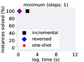
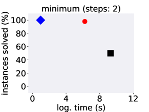
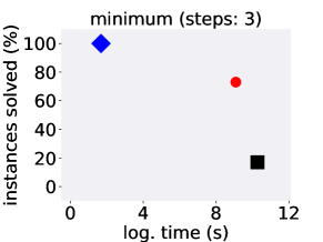
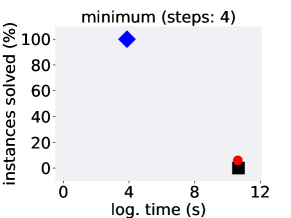
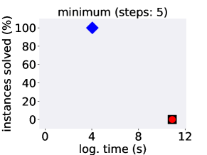
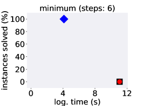
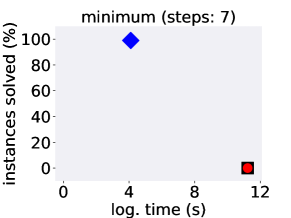
Figure 18: GridWorld: solved instances of minimum explanation search, by (accumulative) time, and $1\leq k\leq 8$ steps.

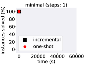
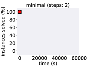
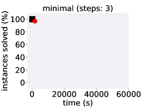
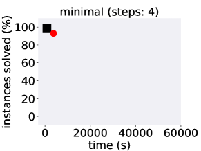
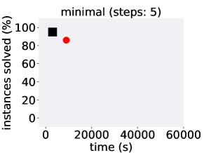
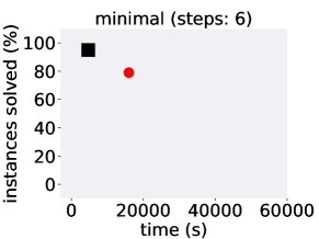
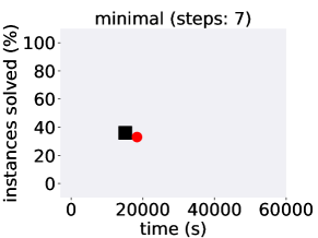
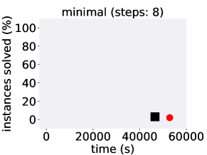
Figure 19: TurtleBot: solved instances of minimal explanation search, by (accumulative) time, and $1\leq k\leq 8$ steps.

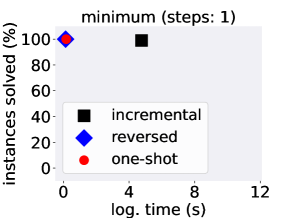
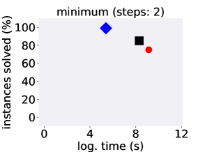
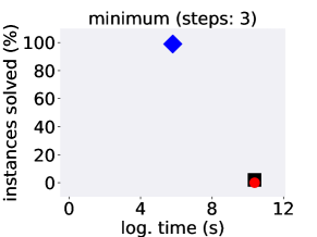
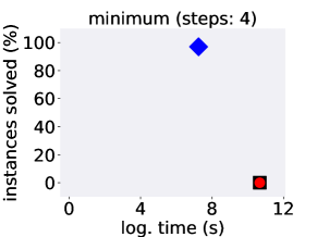
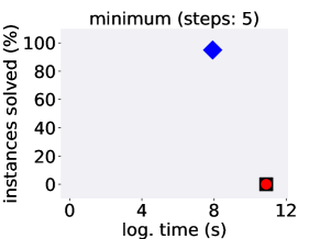
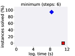
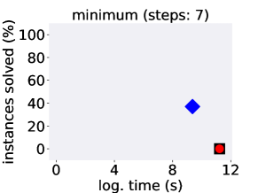
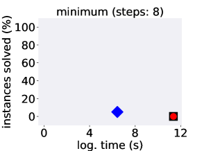
Figure 20: TurtleBot: solved instances of minimum explanation search, by (accumulative) time, and $1\leq k\leq 8$ steps.

8 Comparison to Heuristic XAI Methods

Many heuristic explainable RL (XRL) methods intervene in the training phase [54, 2, 69], and are thus unsuitable for providing a feature-level, post-hoc explanation — and consequently, are incomparable to our approach. Instead, we focused on approaches similar to the ones suggested in [100, 87, 107, 25], which generate explanations for DRL agents using feature-level XAI methods. We studied two popular methods: LIME [85], and SHAP [67]. Specifically, we compared our best-performing method, i.e., the reverse incremental enumeration method (Method 4) to these approaches. We follow common conventions [48] for comparing between these heuristic methods and (our) formal XAI methods — and allow LIME and SHAP to select explanations of the same size as our generated explanations. For each trace, we check whether the explanation produced by these competing methods (on this multi-step sequence) is valid. This is done by checking whether it is a valid hitting set of the produced contrastive examples [47, 46].

Our results (summarized in Table 3) demonstrate the usefulness of our verification-driven method. Although LIME and SHAP are highly scalable, they tend to generate skewed explanations. This is often the case even for a single-step execution. This finding is in line with previous research [48, 20]. In addition, it is apparent that when increasing the number of steps in the execution, the correctness of the explanations provided by these approaches decreases drastically. We believe this is compelling evidence for the significance of our approach in generating formally provable, multi-step explanations of executions, which can only rarely be correctly generated by competing XAI approaches.

Table 3: Comparing non-verification approaches to our formal explainability method. The columns indicate the ratio of correct results, per step.

verified as formal explanations (%)
benchmark	approach	steps (k)
		1	2	3	4	5	6	$\geq$7
GridWorld	LIME	15.0	1.0	2.0	0	0	0	0
	SHAP	2.0	0	0	0	0	0	0
TurtleBot	LIME	20.0	0	0	2.1	1.1	0	0
	SHAP	23.0	2.0	2.0	1.0	0	0	0

References

- [1] A. Albarghouthi. Introduction to Neural Network Verification. verifieddeeplearning.com, 2021.
- [2] D. Amir and O. Amir. Highlights: Summarizing Agent Behavior to People. In Proc. 17th Int. Conf. on Autonomous Agents and Multi Agent Systems (AAMAS), pages 1168–1176, 2018.
- [3] G. Amir, D. Corsi, R. Yerushalmi, L. Marzari, D. Harel, A. Farinelli, and G. Katz. Verifying Learning-Based Robotic Navigation Systems. In Proc. 29th Int. Conf. on Tools and Algorithms for the Construction and Analysis of Systems (TACAS), pages 607–627, 2023.
- [4] G. Amir, Z. Freund, G. Katz, E. Mandelbaum, and I. Refaeli. veriFIRE: Verifying an Industrial, Learning-Based Wildfire Detection System. In Proc. 25th Int. Symposium on Formal Methods (FM), pages 648–656, 2023.
- [5] G. Amir, O. Maayan, T. Zelazny, G. Katz, and M. Schapira. Verifying Generalization in Deep Learning. In Proc. 35th Int. Conf. on Computer Aided Verification (CAV), pages 438–455, 2023.
- [6] G. Amir, M. Schapira, and G. Katz. Towards Scalable Verification of Deep Reinforcement Learning. In Proc. 21st Int. Conf. on Formal Methods in Computer-Aided Design (FMCAD), pages 193–203, 2021.
- [7] G. Amir, H. Wu, C. Barrett, and G. Katz. An SMT-Based Approach for Verifying Binarized Neural Networks. In Proc. 27th Int. Conf. on Tools and Algorithms for the Construction and Analysis of Systems (TACAS), pages 203–222, 2021.
- [8] G. Amir, T. Zelazny, G. Katz, and M. Schapira. Verification-Aided Deep Ensemble Selection. In Proc. 22nd Int. Conf. on Formal Methods in Computer-Aided Design (FMCAD), pages 27–37, 2022.
- [9] G. Anderson, S. Pailoor, I. Dillig, and S. Chaudhuri. Optimization and Abstraction: a Synergistic Approach for Analyzing Neural Network Robustness. In Proc. 40th ACM SIGPLAN Conf. on Programming Languages Design and Implementations (PLDI), pages 731–744, 2019.
- [10] C. Angermueller, T. Pärnamaa, L. Parts, and O. Stegle. Deep Learning for Computational Biology. Molecular Systems Biology, 12(7):878, 2016.
- [11] J. Angwin, J. Larson, S. Mattu, and L. Kirchner. Machine Bias. Ethics of Data and Analytics, pages 254–264, 2016.
- [12] S. Aradi. Survey of Deep Reinforcement Learning for Motion Planning of Autonomous Vehicles. IEEE Transactions on Intelligent Transportation Systems, 2020.
- [13] G. Avni, R. Bloem, K. Chatterjee, T. Henzinger, B. Könighofer, and S. Pranger. Run-Time Optimization for Learned Controllers through Quantitative Games. In Proc. 31st Int. Conf. on Computer Aided Verification (CAV), pages 630–649, 2019.
- [14] T. Baluta, S. Shen, S. Shinde, K. Meel, and P. Saxena. Quantitative Verification of Neural Networks and its Security Applications. In Proc. ACM SIGSAC Conf. on Computer and Communications Security (CCS), pages 1249–1264, 2019.
- [15] P. Barceló, M. Monet, J. Pérez, and B. Subercaseaux. Model Interpretability through the Lens of Computational Complexity. In Proc. 33rd Conf. on Neural Information Processing Systems (NeurIPS), 2020.
- [16] S. Bassan, G. Amir, D. Corsi, I. Refaeli, and G. Katz. Formally Explaining Neural Networks within Reactive Systems: Artifact, 2023. https://zenodo.org/record/8197762.
- [17] S. Bassan and G. Katz. Towards Formal Approximated Minimal Explanations of Neural Networks. In Proc. 29th Int. Conf. on Tools and Algorithms for the Construction and Analysis of Systems (TACAS), pages 187–207, 2023.
- [18] L. Brunke, M. Greeff, A. Hall, Z. Yuan, S. Zhou, J. Panerati, and A. Schoellig. Safe Learning in Robotics: From Learning-Based Control to Safe Reinforcement Learning. Annual Review of Control, Robotics, and Autonomous Systems, 5:411–444, 2022.
- [19] CACM Staff. A Case Against Mission-Critical Applications of Machine Learning. Communications of the ACM, 62(8):9–9, 2019.
- [20] O. Camburu, E. Giunchiglia, J. Foerster, T. Lukasiewicz, and P. Blunsom. Can I Trust the Explainer? Verifying Post-Hoc Explanatory Methods, 2019. Technical Report. http://arxiv.org/abs/1910.02065.
- [21] M. Casadio, E. Komendantskaya, M. Daggitt, W. Kokke, G. Katz, G. Amir, and I. Refaeli. Neural Network Robustness as a Verification Property: A Principled Case Study. In Proc. 34th Int. Conf. on Computer Aided Verification (CAV), pages 219–231, 2022.
- [22] D. Corsi, E. Marchesini, and A. Farinelli. Formal Verification of Neural Networks for Safety-Critical Tasks in Deep Reinforcement Learning. In Proc. 37th Int. Conf. on Uncertainty in Artificial Intelligence (UAI), 2021.
- [23] D. Corsi, L. Marzari, A. Pore, A. Farinelli, A. Casals, P. Fiorini, and D. Dall’Alba. Constrained Reinforcement Learning and Formal Verification for Safe Colonoscopy Navigation. In Proc. IEEE Int. Conf. on Intelligent Robots and Systems (IROS), 2023.
- [24] D. Corsi, R. Yerushalmi, G. Amir, A. Farinelli, D. Harel, and G. Katz. Constrained Reinforcement Learning for Robotics via Scenario-Based Programming, 2022. Technical Report. https://arxiv.org/abs/2206.09603.
- [25] A. Dethise, M. Canini, and S. Kandula. Cracking Open the Black Box: What Observations Can Tell Us About Reinforcement Learning Agents. In Proc. 2019 Workshop on Network Meets AI & ML, pages 29–36, 2019.
- [26] J. Devlin, M.-W. Chang, K. Lee, and K. Toutanova. Bert: Pre-Training of Deep Bidirectional Transformers for Language Understanding, 2018. Technical Report. https://arxiv.org/abs/1810.04805.
- [27] T. Eliyahu, Y. Kazak, G. Katz, and M. Schapira. Verifying Learning-Augmented Systems. In Proc. Annual Conf. of the ACM Special Interest Group on Data Communication on the Applications, Technologies, Architectures, and Protocols for Computer Communication (SIGCOMM), 2021.
- [28] T. Fel, M. Ducoffe, D. Vigouroux, R. Cadène, M. Capelle, C. Nicodème, and T. Serre. Don’t Lie to Me! Robust and Efficient Explainability with Verified Perturbation Analysis, 2022. Technical Report. https://arxiv.org/abs/2202.07728.
- [29] T. Gehr, M. Mirman, D. Drachsler-Cohen, E. Tsankov, S. Chaudhuri, and M. Vechev. AI2: Safety and Robustness Certification of Neural Networks with Abstract Interpretation. In Proc. 39th IEEE Symposium on Security and Privacy (S&P), 2018.
- [30] C. Geng, N. Le, X. Xu, Z. Wang, A. Gurfinkel, and X. Si. Toward Reliable Neural Specifications, 2022. Technical Report. https://arxiv.org/abs/2210.16114.
- [31] I. Goodfellow, J. Shlens, and C. Szegedy. Explaining and Harnessing Adversarial Examples, 2014. Technical Report. http://arxiv.org/abs/1412.6572.
- [32] D. Gopinath, G. Katz, C. Pǎsǎreanu, and C. Barrett. DeepSafe: A Data-Driven Approach for Checking Adversarial Robustness in Neural Networks. In Proc. 16th. Int. Symp. on on Automated Technology for Verification and Analysis (ATVA), pages 3–19, 2018.
- [33] D. Guidotti, L. Pulina, and A. Tacchella. pyNeVer: A Framework for Learning and Verification of Neural Networks. In Proc. 19th. Int. Symposium on Automated Technology for Verification and Analysis (ATVA), pages 357–363, 2021.
- [34] D. Gunning, M. Stefik, J. Choi, T. Miller, S. Stumpf, and G.-Z. Yang. XAI—Explainable Artificial Intelligence. Science Robotics, 4(37):eaay7120, 2019.
- [35] A. Heuillet, F. Couthouis, and N. Díaz-Rodríguez. Explainability in Deep Reinforcement Learning. Knowledge-Based Systems, 214:106685, 2021.
- [36] R. Hoffman, S. Mueller, G. Klein, and J. Litman. Metrics for Explainable AI: Challenges and Prospects, 2018. Technical Report. https://arxiv.org/abs/1812.04608.
- [37] X. Huang, M. Cooper, A. Morgado, J. Planes, and J. Marques-Silva. Feature Necessity & Relevancy in ML Classifier Explanations. In Proc. 29th Int. Conf. on Tools and Algorithms for the Construction and Analysis of Systems (TACAS), pages 167–186, 2023.
- [38] X. Huang, Y. Izza, A. Ignatiev, and J. Marques-Silva. On Efficiently Explaining Graph-Based Classifiers, 2021. Technical Report. https://arxiv.org/abs/2106.01350.
- [39] X. Huang, M. Kwiatkowska, S. Wang, and M. Wu. Safety Verification of Deep Neural Networks. In Proc. 29th Int. Conf. on Computer Aided Verification (CAV), pages 3–29, 2017.
- [40] X. Huang and J. Marques-Silva. From Robustness to Explainability and Back Again, 2023. Technical Report. https://arxiv.org/abs/2306.03048.
- [41] IBM. The CPLEX optimizer, 2018.
- [42] A. Ignatiev. Towards Trustable Explainable AI. In Proc. 29th Int. Joint Conf. on Artificial Intelligence (IJCAI), pages 5154–5158, 2020.
- [43] A. Ignatiev and J. Marques-Silva. SAT-Based Rigorous Explanations for Decision Lists. In Proc. 24th Int. Conf. on Theory and Applications of Satisfiability Testing (SAT), pages 251–269, 2021.
- [44] A. Ignatiev, A. Morgado, and J. Marques-Silva. Propositional Abduction with Implicit Hitting Sets, 2016. Technical Report. http://arxiv.org/abs/1604.08229.
- [45] A. Ignatiev, A. Morgado, and J. Marques-Silva. PySAT: A Python Toolkit for Prototyping with SAT Oracles. In Proc. 21st Int. Conf. on Theory and Applications of Satisfiability Testing (SAT), pages 428–437, 2018.
- [46] A. Ignatiev, N. Narodytska, N. Asher, and J. Marques-Silva. From Contrastive to Abductive Explanations and Back Again. In Proc. 19th Int. Conf. of the Italian Association for Artificial Intelligence (AIxIA), pages 335–355, 2020.
- [47] A. Ignatiev, N. Narodytska, and J. Marques-Silva. Abduction-Based Explanations for Machine Learning Models. In Proc. 33rd AAAI Conf. on Artificial Intelligence (AAAI), pages 1511–1519, 2019.
- [48] A. Ignatiev, N. Narodytska, and J. Marques-Silva. On Validating, Repairing and Refining Heuristic ML Explanations, 2019. Technical Report. http://arxiv.org/abs/1907.02509.
- [49] A. Ignatiev, F. Pereira, N. Narodytska, and J. Marques-Silva. A SAT-Based Approach to Learn Explainable Decision Sets. In Proc. 9th Int. Joint Conf. on Automated Reasoning (IJCAR), pages 627–645, 2018.
- [50] A. Ignatiev, A. Previti, M. Liffiton, and J. Marques-Silva. Smallest MUS Extraction with Minimal Hitting Set Dualization. In Proc. 21st Int. Conf. on Principles and Practice of Constraint Programming (CP), pages 173–182, 2015.
- [51] Y. Izza, A. Ignatiev, and J. Marques-Silva. On Explaining Decision Trees, 2020. Technical Report. http://arxiv.org/abs/2010.11034.
- [52] Y. Izza, A. Ignatiev, N. Narodytska, M. Cooper, and J. Marques-Silva. Efficient Explanations with Relevant Sets, 2021. Technical Report. http://arxiv.org/abs/2106.00546.
- [53] Y. Jacoby, C. Barrett, and G. Katz. Verifying Recurrent Neural Networks using Invariant Inference. In Proc. 18th Int. Symposium on Automated Technology for Verification and Analysis (ATVA), pages 57–74, 2020.
- [54] Z. Juozapaitis, A. Koul, A. Fern, M. Erwig, and F. Doshi-Velez. Explainable Reinforcement Learning via Reward Decomposition. In Proc. IJCAI/ECAI Workshop on Explainable Artificial Intelligence, 2019.
- [55] G. Katz, C. Barrett, D. Dill, K. Julian, and M. Kochenderfer. Reluplex: An Efficient SMT Solver for Verifying Deep Neural Networks. In Proc. 29th Int. Conf. on Computer Aided Verification (CAV), pages 97–117, 2017.
- [56] G. Katz, D. Huang, D. Ibeling, K. Julian, C. Lazarus, R. Lim, P. Shah, S. Thakoor, H. Wu, A. Zeljić, D. Dill, M. Kochenderfer, and C. Barrett. The Marabou Framework for Verification and Analysis of Deep Neural Networks. In Proc. 31st Int. Conf. on Computer Aided Verification (CAV), pages 443–452, 2019.
- [57] B. Könighofer, F. Lorber, N. Jansen, and R. Bloem. Shield Synthesis for Reinforcement Learning. In Proc. Int. Symposium on Leveraging Applications of Formal Methods, Verification and Validation (ISoLA), pages 290–306, 2020.
- [58] A. Krizhevsky, I. Sutskever, and G. Hinton. Imagenet Classification with Deep Convolutional Neural Networks. In Proc. 30rd Conf. on Neural Information Processing Systems (NeurIPS), 2017.
- [59] E. La Malfa, A. Zbrzezny, R. Michelmore, N. Paoletti, and M. Kwiatkowska. On Guaranteed Optimal Robust Explanations for NLP Models, 2021. Technical Report. https://arxiv.org/abs/2105.03640.
- [60] O. Lahav and G. Katz. Pruning and Slicing Neural Networks using Formal Verification. In Proc. 21st Int. Conf. on Formal Methods in Computer-Aided Design (FMCAD), pages 183–192, 2021.
- [61] Y. LeCun, Y. Bengio, and G. Hinton. Deep Learning. Nature, 521(7553):436–444, 2015.
- [62] A. Lekharu, K. Moulii, A. Sur, and A. Sarkar. Deep Learning Based Prediction Model for Adaptive Video Streaming. In Proc. Int. Conf. on Communication Systems & NETworkS (COMSNETS), pages 152–159, 2020.
- [63] C. Li and F. Manya. MaxSAT, Hard and Soft Constraints. In Handbook of Satisfiability, pages 903–927. IOS Press, 2021.
- [64] Y. Li. Deep Reinforcement Learning: An Overview, 2017. Technical Report. http://arxiv.org/abs/1701.07274.
- [65] P. Liberatore. Redundancy in Logic I: CNF Propositional Formulae. Artificial Intelligence, 163(2):203–232, 2005.
- [66] C. Liu, T. Arnon, C. Lazarus, C. Barrett, and M. Kochenderfer. Algorithms for Verifying Deep Neural Networks, 2020. Technical Report. http://arxiv.org/abs/1903.06758.
- [67] S. Lundberg and S.-I. Lee. A Unified Approach to Interpreting Model Predictions. In Proc. 31st Conf. on Neural Information Processing Systems (NeurIPS), 2017.
- [68] N. Luong, D. Hoang, S. Gong, D. Niyato, P. Wang, Y.-C. Liang, and D. Kim. Applications of Deep Reinforcement Learning in Communications and Networking: A Survey. IEEE Communications Surveys & Tutorials, 21(4):3133–3174, 2019.
- [69] P. Madumal, T. Miller, L. Sonenberg, and F. Vetere. Explainable Reinforcement Learning through a Causal Lens. In Proc. 34th AAAI Conf. on Artificial Intelligence (AAAI), pages 2493–2500, 2020.
- [70] E. Marchesini, D. Corsi, and A. Farinelli. Exploring Safer Behaviors for Deep Reinforcement Learning. In Proc. 35th AAAI Conf. on Artificial Intelligence (AAAI), 2021.
- [71] J. Marques-Silva, T. Gerspacher, M. Cooper, A. Ignatiev, and N. Narodytska. Explaining Naive Bayes and Other Linear Classifiers with Polynomial Time and Delay. In Proc. 33rd Conf. on Neural Information Processing Systems (NeurIPS), pages 20590–20600, 2020.
- [72] J. Marques-Silva and A. Ignatiev. Delivering Trustworthy AI through formal XAI. In Proc. 36th AAAI Conf. on Artificial Intelligence (AAAI), pages 3806–3814, 2022.
- [73] L. Marzari, D. Corsi, F. Cicalese, and A. Farinelli. The #DNN-Verification Problem: Counting Unsafe Inputs for Deep Neural Networks. In Proc. 32nd Int. Joint Conf. on Artificial Intelligence (IJCAI), 2023.
- [74] K. McMillan. Bayesian Interpolants as Explanations for Neural Inferences, 2020. Technical Report. https://arxiv.org/abs/2004.04198.
- [75] V. Mnih, K. Kavukcuoglu, D. Silver, A. Graves, I. Antonoglou, D. Wierstra, and M. Riedmiller. Playing Atari with Deep Reinforcement Learning, 2013. Technical Report. https://arxiv.org/abs/1312.5602.
- [76] M. Müller, G. Makarchuk, G. Singh, M. Püschel, and M. Vechev. PRIMA: General and Precise Neural Network Certification via Scalable Convex Hull Approximations, 2021. Technical Report. https://arxiv.org/abs/2103.03638.
- [77] T. Okudono, M. Waga, T. Sekiyama, and I. Hasuo. Weighted Automata Extraction from Recurrent Neural Networks via Regression on State Spaces. In Proc. 34th AAAI Conf. on Artificial Intelligence (AAAI), pages 5037–5044, 2020.
- [78] M. Ostrovsky, C. Barrett, and G. Katz. An Abstraction-Refinement Approach to Verifying Convolutional Neural Networks. In Proc. 20th. Int. Symposium on Automated Technology for Verification and Analysis (ATVA), pages 391–396, 2022.
- [79] E. Polgreen, R. Abboud, and D. Kroening. Counterexample Guided Neural Synthesis, 2020. Technical Report. https://arxiv.org/abs/2001.09245.
- [80] A. Pore, D. Corsi, E. Marchesini, D. Dall’Alba, A. Casals, A. Farinelli, and P. Fiorini. Safe Reinforcement Learning using Formal Verification for Tissue Retraction in Autonomous Robotic-Sssisted Surgery. In Proc. IEEE/RSJ Int. Conf. on Intelligent Robots and Systems (IROS), 2021.
- [81] P. Prabhakar and Z. Afzal. Abstraction Based Output Range Analysis for Neural Networks, 2020. Technical Report. https://arxiv.org/abs/2007.09527.
- [82] E. Puiutta and E. Veith. Explainable Reinforcement Learning: A Survey. In Proc. Int. Cross-Domain Conf. for Machine Learning and Knowledge Extraction (CD-MAKE), pages 77–95, 2020.
- [83] I. Refaeli and G. Katz. Minimal Multi-Layer Modifications of Deep Neural Networks. In Proc. 5th Workshop on Formal Methods for ML-Enabled Autonomous Systems (FoMLAS), 2022.
- [84] R. Reiter. A Theory of Diagnosis from First Principles. Artificial Intelligence, 32(1):57–95, 1987.
- [85] M. Ribeiro, S. Singh, and C. Guestrin. “Why should I Trust You?” Explaining the Predictions of any Classifier. In Proc. 22nd Int. Conf. on Knowledge Discovery and Data Mining (KDD), pages 1135–1144, 2016.
- [86] M. Ribeiro, S. Singh, and C. Guestrin. Anchors: High-Precision Model-Agnostic Explanations. In Proc. 32nd AAAI Conf. on Artificial Intelligence (AAAI), 2018.
- [87] S. Rizzo, G. Vantini, and S. Chawla. Reinforcement Learning with Explainability for Traffic Signal Control. In Proc. IEEE Intelligent Transportation Systems Conference (ITSC), pages 3567–3572, 2019.
- [88] J. Schulman, F. Wolski, P. Dhariwal, A. Radford, and O. Klimov. Proximal Policy Optimization Algorithms, 2017. Technical Report. http://arxiv.org/abs/1707.06347.
- [89] R. Selvaraju, M. Cogswell, A. Das, R. Vedantam, D. Parikh, and D. Batra. Grad-Cam: Visual Explanations from Deep Networks via Gradient-Based Localization. In Proc. 20th IEEE Int. Conf. on Computer Vision (ICCV), pages 618–626, 2017.
- [90] S. Seshia, A. Desai, T. Dreossi, D. Fremont, S. Ghosh, E. Kim, S. Shivakumar, M. Vazquez-Chanlatte, and X. Yue. Formal Specification for Deep Neural Networks. In Proc. 16th Int. Symposium on Automated Technology for Verification and Analysis (ATVA), pages 20–34, 2018.
- [91] M. Shahbaz and R. Groz. Inferring Mealy Machines. In Proc. Conf. on Formal Methods (FM), pages 207–222, 2009.
- [92] W. Shi, A. Shih, A. Darwiche, and A. Choi. On Tractable Representations of Binary Neural Networks, 2020. Technical Report. http://arxiv.org/abs/2004.02082.
- [93] A. Shih, A. Choi, and A. Darwiche. A Symbolic Approach to Explaining Bayesian Network Classifiers, 2018. Technical Report. http://arxiv.org/abs/1805.03364.
- [94] D. Silver, J. Schrittwieser, K. Simonyan, I. Antonoglou, A. Huang, A. Guez, T. Hubert, L. Baker, M. Lai, A. Bolton, et al. Mastering the Game of Go Without Human Knowledge. nature, 550(7676):354–359, 2017.
- [95] M. Sotoudeh and A. Thakur. Correcting Deep Neural Networks with Small, Generalizing Patches. In Proc. Workshop on Safety and Robustness in Decision Making, 2019.
- [96] J. Su, D. Vargas, and K. Sakurai. One Pixel Attack for Fooling Deep Neural Networks. IEEE Transactions on Evolutionary Computation, 23(5):828–841, 2019.
- [97] R. Sutton and A. Barto. Reinforcement Learning: An Introduction. MIT press, 2018.
- [98] R. Sutton, D. McAllester, S. Singh, and Y. Mansour. Policy Gradient Methods for Reinforcement Learning with Function Approximation. In Proc. 12th Conf. on Advances in Neural Information Processing Systems (NeurIPS), 1999.
- [99] L. Tai, G. Paolo, and M. Liu. Virtual-to-Real Deep Reinforcement Learning: Continuous Control of Mobile Robots for Mapless Navigation. In Proc. IEEE/RSJ Int. Conf. on Intelligent Robots and Systems (IROS), 2017.
- [100] G. Vouros. Explainable Deep Reinforcement Learning: State of the Art and Challenges. ACM Computing Surveys, 55(5):1–39, 2022.
- [101] S. Waeldchen, J. Macdonald, S. Hauch, and G. Kutyniok. The Computational Complexity of Understanding Binary Classifier Decisions. Journal of Artificial Intelligence Research, 70:351–387, 2021.
- [102] S. Wang, H. Zhang, K. Xu, X. Lin, S. Jana, C.-J. Hsieh, and J. Z. Kolter. Beta-Crown: Efficient Bound Propagation with Per-Neuron Split Constraints for Neural Network Robustness Verification. In Proc. 34th Conf. on Neural Information Processing Systems (NeurIPS), volume 34, pages 29909–29921, 2021.
- [103] H. Wu, A. Ozdemir, A. Zeljić, A. Irfan, K. Julian, D. Gopinath, S. Fouladi, G. Katz, C. Păsăreanu, and C. Barrett. Parallelization Techniques for Verifying Neural Networks. In Proc. 20th Int. Conf. on Formal Methods in Computer-Aided Design (FMCAD), pages 128–137, 2020.
- [104] M. Wu, H. Wu, and C. Barrett. VeriX: Towards Verified Explainability of Deep Neural Networks, 2022. Technical Report. https://arxiv.org/abs/2212.01051.
- [105] H. Zhang, M. Shinn, A. Gupta, A. Gurfinkel, N. Le, and N. Narodytska. Verification of Recurrent Neural Networks for Cognitive Tasks via Reachability Analysis. In Proc. 24th European Conf. on Artificial Intelligence (ECAI), pages 1690–1697, 2020.
- [106] J. Zhang, Y. Liu, K. Zhou, G. Li, Z. Xiao, B. Cheng, J. Xing, Y. Wang, T. Cheng, L. Liu, et al. An End-to-End Automatic Cloud Database Tuning System using Deep Reinforcement Learning. In Proc. Int. Conf. on Management of Data (SIGMOD), pages 415–432, 2019.
- [107] K. Zhang, P. Xu, and J. Zhang. Explainable AI in Deep Reinforcement Learning Models: A Shap Method Applied in Power System Emergency Control. In Proc. 4th IEEE Conf. on Energy Internet and Energy System Integration (EI2), pages 711–716, 2020.
- [108] Z. Zhou and L. Sun. Metamorphic Testing of Driverless Cars. Communications of the ACM, 62(3):61–67, 2019.