Vicsek Model Meets DBSCAN: Cluster Phases in the Vicsek Model

Abstract

The Vicsek model, which was originally proposed to explain the dynamics of bird flocking, exhibits a phase transition with respect to the absolute value of the mean velocity. Although clusters of agents can be easily observed via numerical simulations of the Vicsek model, qualitative studies are lacking. We study the clustering structure of the Vicsek model by applying DBSCAN, a recently-introduced clustering algorithm, and report that the Vicsek model shows a phase transition with respect to the number of clusters: from $\mathcal{O}(N)$ to $\mathcal{O}(1)$, with $N$ being the number of agents, when increasing the magnitude of noise for a fixed radius that specifies the interaction of the Vicsek model. We also report that the combination of the order parameter proposed by Vicsek et al. and the number of clusters defines at least four phases of the Vicsek model.

I Introduction

The dynamics of self-propelling agents, often referred to as active matter, has attracted much attention since the discovery of the phase transition of the Vicsek model, which was originally proposed as a model of bird flocking [1, 2, 3, 4]. Active matter covers a wide range of systems, including animal flocks [5], bacterial colonies [6], molecular motors [7], tissue dynamics [8], crowd dynamics [9, 8], collective motion in rare events [10], collective motion in disordered systems [11], and nonreciprocal systems [12, 13], and so far numerical simulations have been performed to investigate systems these systems. In addition to numerical studies, nonequilibrium statistical-mechanical approaches based on the Boltzmann equation and the hydrodynamic approach have also contributed to clarifying the nature of active matter and the dynamics of self-propelling agents [14, 15, 16, 17]. Motivated by topological condensed matter physics, the study of the robust structure of active matter, known as topological active matter systems, is also an area of active research [18].

Another important trend that is accelerating research in active matter is machine learning [19, 20]. Recent studies on the application of machine learning to active matter are discussed in Refs. [21, 22, 23, 24]. In particular, clustering algorithms are of special significance since clustering structures appear ubiquitously in science and engineering, including active matter. Reference [25] summarizes several clustering algorithms – both well-known ones, as well as those that have been introduced recently – such as $k$-means, the EM algorithm with the Gaussian mixture model [26, 27], OPTICS [28], agglomerative clustering, and DBSCAN (density based spatial clustering of applications with noise) [29]. Depending on the choice of clustering algorithms, estimates of clusters present in a given data set can drastically change and often fail to capture the correct structure. More importantly, research on cluster phases in active matter is still limited [30, 31, 32].

In this paper, we investigate the clustering structure of the Vicsek model by applying DBSCAN, a recently-introduced clustering algorithm inspired by topological properties of data sets [29]. First, we state a mathematical connection between the Vicsek model and DBSCAN by rewriting the Vicsek model in the form of the overdamped Langevin equation and then showing that one can identify a cost function of DBSCAN that matches the potential function of a Vicsek model. We then report our numerical results showing that the Vicsek model exhibits phase transitions in the number of clusters, as determined by DBSCAN. Specifically, we observe a phase transition from $\mathcal{O}(N)$ to $\mathcal{O}(1)$ in the dependence of the number of clusters on the number of agents for a fixed density, as the magnitude of noise is increased for a fixed radius that specifies the interaction among agents in the Vicsek model. Additionally, by combining the order parameter proposed in Ref. [1], we identify multiple phases in the Vicsek model.

The rest of this paper is organized as follows. In Sec. II, we introduce the Vicsek model [1]. In Sec. III, we explain DBSCAN [29]. In Sec. IV, we show numerical simulations of the Vicsek model and the results of DBSCAN. In Sec. V, we discuss the numerical simulations using the schematic picture of the phases of the Vicsek model. Finally, Sec. VI summarize our findings and concludes this paper.

II Vicsek model

We first introduce the Vicsek model [1], which was proposed as a possible explanation for bird flocking and has been successful in describing the phase transition of agents forming a flock. Next, we derive its continuous-time variant, also known as the overdamped Langevin equation, and the potential energy of the Vicsek model. This potential energy is minimized via the overdamped Langevin equation of the Vicsek model. The potential energy of the Vicsek model plays an important role in discussing the correspondence between the Vicsek model and DBSCAN.

II.1 Definition

Let us consider a two-dimensional system of $n_{\mathrm{ag}}$ self-propelling agents. We denote, by $\bm{x}_{i}(t)$ and $\bm{v}_{i}(t)$, the position and velocity of agent $i$ at time $t$, respectively. The direction of $\bm{v}_{i}(t)$ is computed as

$$\bm{v}_{i}(t) =v_{\mathrm{abs}}\begin{bmatrix}\cos\theta_{i}(t)\\ \sin\theta_{i}(t)\end{bmatrix},$$ (2.1)

and

$$\theta_{i}(t+\Delta t) =\frac{1}{N_{i,r_{\mathrm{V}}}}\sum_{\begin{subarray}{c}j:\\ \|\bm{x}_{i}(t)-\bm{x}_{j}(t)\|_{\mathrm{F}}<r_{\mathrm{V}}\end{subarray}}\theta_{j}(t)+\Xi_{i}(t),$$ (2.2)

$$\Xi_{i}(t) \sim[-\eta/2,\eta/2],$$ (2.3)

where $N_{i,r_{\mathrm{V}}}$ is the number of elements that satisfy $\|\bm{x}_{i}(t)-\bm{x}_{j}(t)\|_{\mathrm{F}}<r_{\mathrm{V}}$, while the magnitude of the velocity of each agent is constant: $\|\bm{v}_{i}(t)\|_{\mathrm{F}}=v_{\mathrm{abs}}$ where $\|\cdot\|_{\mathrm{F}}$ is the Frobenius norm. Then the position of agent $i$ is updated by

$$\bm{x}_{i}(t+\Delta t) =\bm{x}_{i}(t)+\bm{v}_{i}(t)\Delta t.$$ (2.4)

Eq. (2.2) is often called the metric interaction since the summation is taken over all the agents that satisfy the metric condition. Eq. (2.3) means $\Xi_{i}(t)$ is randomly sampled from the uniform distribution whose upper and lower bounds are $\eta/2$ and $-\eta/2$, respectively. Note that the variance of this uniform distribution is $\eta^{2}/12$.

II.2 Overdamped Langevin equation for the Vicsek model

For small $\Delta t$, we can use the following approximation:

$$\theta_{i}(t+\Delta t) \approx\theta_{i}(t)+\frac{d}{dt}\theta_{i}(t)\cdot\Delta t.$$ (2.5)

From Eq. (2.2) and (2.5), we have

$$\frac{d}{dt}\theta_{i}(t) =\frac{1}{N_{i,r_{\mathrm{V}}}\Delta t}\sum_{\begin{subarray}{c}j:\\ \|\bm{x}_{i}(t)-\bm{x}_{j}(t)\|_{\mathrm{F}}<r_{\mathrm{V}}\end{subarray}}\theta_{j}(t)-\frac{\theta_{i}(t)}{\Delta t}+\xi(t).$$ (2.6)

where $N_{i,r_{\mathrm{V}}}$ is the number of elements ($j$) that satisfy $\|\bm{x}_{i}-\bm{x}_{j}\|_{\mathrm{F}}\leq r_{\mathrm{V}}$ and $\xi(t)\coloneqq\frac{d}{dt}\Xi(t)$.

Assuming $N_{i,r_{\mathrm{V}}}=N_{j,r_{\mathrm{V}}}$ for $i$ and $j$ that belongs to the same cluster, we can rewrite Eq. (2.6) in the following form:

$$\frac{d}{dt}\theta_{i}(t) =-\frac{\partial}{\partial\theta_{i}}V_{r_{\mathrm{V}}}(\{\theta_{i}\}_{i=1}^{n_{\mathrm{ag}}})\bigg{|}_{\{\theta_{i}\}_{i=1}^{n_{\mathrm{ag}}}=\{\theta_{i}(t)\}_{i=1}^{n_{\mathrm{ag}}}}+\xi(t),$$ (2.7)

where

$$V_{r_{\mathrm{V}}}(\{\theta_{i}\}_{i=1}^{n_{\mathrm{ag}}}) \coloneqq-\frac{1}{2\Delta t}\sum_{i=1}^{n_{\mathrm{ag}}}\frac{1}{N_{i,r_{\mathrm{V}}}}\theta_{i}\bBigg@{4.0}(\sum_{\begin{subarray}{c}j:\\ \|\bm{x}_{i}-\bm{x}_{j}\|_{\mathrm{F}}\leq r_{\mathrm{V}}\end{subarray}}\theta_{j}\bBigg@{4.0}$$

$$\quad+\frac{1}{2\Delta t}\theta_{i}^{2}$$ (2.8)

$$=-\frac{1}{2}\sum_{i=1}^{n_{\mathrm{ag}}}\sum_{\begin{subarray}{c}j:\\ \|\bm{x}_{i}-\bm{x}_{j}\|_{\mathrm{F}}\leq r_{\mathrm{V}}\end{subarray}}\frac{\theta_{i}\theta_{j}}{N_{i,r_{\mathrm{V}}}}+\frac{1}{2\Delta t}\theta_{i}^{2}.$$ (2.9)

In the Vicsek model, Eq. (2.9) is minimized via Eq. (2.7). Note that the condition of $N_{i,r_{\mathrm{V}}}=N_{j,r_{\mathrm{V}}}$ for $i$ and $j$ that belongs to the same cluster is not assumed in the Vicsek model and it implies that the interaction of the Vicsek model is not reciprocal.

II.3 Order parameter of the Vicsek model

In Ref. [1], the following function was investigated as the order parameter:

$$v_{\mathrm{op}}(t) \coloneqq\frac{1}{v_{\mathrm{abs}}n_{\mathrm{ag}}}\bigg{\|}\sum_{i=1}^{n_{\mathrm{ag}}}\bm{v}_{i}(t)\bigg{\|}_{\mathrm{F}}.$$ (2.10)

Vicsek et al. reported that Eq. (2.10) describes the phase transition of the Vicsek model.

III DBSCAN

To investigate the clustering structure of the Vicsek model, we apply DBSCAN to the Vicsek model. We first review DBSCAN [29, 33, 34, 35, 36]. Then, we derive a cost function of DBSCAN. To the best of our knowledge, the cost function of DBSCAN has not been explicitly stated in the literature. We show a correspondence between the cost function of DBSCAN and the potential function derived for the Vicsek model in the previous section. This correspondence also explains why we have chosen DBSCAN. At the end of this section, we introduce new order parameters to define new phases of the Vicsek model.

III.1 Algorithm

Clustering is an important task in many fields, and many different algorithms have been proposed [25]. Among these, DBSCAN  is widely used [29, 33, 34, 35, 36]. In this section, we describe the problem setting and the novelties of this approach. Let $D_{\mathrm{all}}\coloneqq\{\bm{x}_{i}\}_{i=1}^{n_{\mathrm{ag}}}$ be the dataset comprising $n_{\mathrm{ag}}$ data points. The problem is to estimate $\{l_{i}\}_{i=1}^{n_{\mathrm{ag}}}$, where $l_{i}\in\{0,1,2,\dots,n_{\mathrm{cl}}\}$ is the label of the $i$-th data point, with $l_{i}\geq 1$ meaning that the $i$-th data point belongs to the $l_{i}$-th cluster, and $l_{i}=0$ meaning that the $i$-th data point is an outlier and does not belong to any of the clusters (numbered, $1,\ldots,n_{\mathrm{cl}})$. There are two key points in this problem setting. The first is to estimate the number of clusters, $n_{\mathrm{cl}}$, which is not a given number as in the $k$-means algorithm. The second is that data points may be outliers, denoted by $l_{i}=0$. This feature allows one to estimate a robust clustering structure.

Before delving into the details of DBSCAN, let us introduce the parameters of DBSCAN and explain the underlying concept behind DBSCAN. The first parameter is the radius $r_{\mathrm{D}}$ that defines the neighbors of each data point, and the second parameter is the minimum number of data points $n_{\mathrm{min}}$ that each cluster must have. Otherwise, data points are recognized as outliers. Additionally, we must specify a metric function for DBSCAN. In this paper, we focus on the Euclidean distance. The fundamental concept of DBSCAN is to classify data points into three categories: core points, border points, and outliers. Core points have $n_{\mathrm{min}}$ or more neighbors, border points are reachable from core points but have fewer neighbors than $n_{\mathrm{min}}$, and outliers are not reachable from any data point that belongs to a cluster. Moreover, core points and border points that belong to a cluster must form a cluster of which the number of agents is $n_{\mathrm{min}}$ or more.

We now describe the details of DBSCAN. At the beginning of DBSCAN, we create the sets of visited data points $D_{\mathrm{vst}}$ and outliers $D_{\mathrm{out}}$ and initialize the two sets to the empty set: $D_{\mathrm{vst}}=\emptyset$ and $D_{\mathrm{out}}=\emptyset$. We also set $n_{\mathrm{cl}}=0$, where $n_{\mathrm{cl}}$ is the number of clusters. Then, we randomly pick a data point from $D_{\mathrm{all}}\backslash D_{\mathrm{vst}}$ and run the following main loop. In the main loop, we first add the selected data point to $D_{\mathrm{vst}}$ and compute the $r_{\mathrm{D}}$-neighbors of the selected data point. We refer to the set of $r_{\mathrm{D}}$-neighbors of the selected data point as $D_{\mathrm{ngh}}$. If the number of elements in $D_{\mathrm{ngh}}$ is smaller than $n_{\mathrm{min}}$, then the data points in $D_{\mathrm{ngh}}$ are added to $D_{\mathrm{out}}$. Otherwise, we create a new cluster, increment $n_{\mathrm{cl}}$ by one, add the data points in $D_{\mathrm{ngh}}$ to the new cluster, and expand $D_{\mathrm{ngh}}$ by adding neighbors of $D_{\mathrm{ngh}}\backslash\bm{x}$ as much as possible. We repeat the above main loop until $D_{\mathrm{all}}\backslash D_{\mathrm{vst}}=\emptyset$. The role of the main loop is to find a core point and expand a cluster associated with the core point as much as possible. Note that the first conditional branch of the main loop distinguishes core points from reachable points and outliers. In Algo. 1, the pseudocode of DBSCAN is shown [33, 34, 35]. Therein, two subroutines are used. In Algos. 2 and 3, $\mathrm{region\_query}(\bm{x},r_{\mathrm{D}})$ and $\mathrm{expand\_cluster}(\bm{x},\{C_{k}\}_{k=1}^{n_{\mathrm{cl}}},D_{\mathrm{vst}},r_{\mathrm{D}},n_{\mathrm{min}})$ are shown, respectively. Note that, by definition, $\bm{x}\in\mathrm{region\_query}(\bm{x},r_{\mathrm{D}})$ is always satisfied.

Input : Data set $D_{\mathrm{all}}\coloneqq\{\bm{x}_{i}\}_{i=1}^{n_{\mathrm{ag}}}$, radisu $r_{\mathrm{D}}$, minimum number of nodes in any cluster $n_{\mathrm{min}}$

Output : Label set $\{l_{i}\}_{i=1}^{n_{\mathrm{ag}}}$

1 set $D_{\mathrm{vst}}=\emptyset$, $D_{\mathrm{out}}=\emptyset$, and $n_{\mathrm{cl}}=0$

2 set $l_{i}=0$ for $i=1,2,\dots,n_{\mathrm{ag}}$

3 for $\bm{x}\in D_{\mathrm{all}}\backslash D_{\mathrm{vst}}$ do

4       $D_{\mathrm{vst}}\leftarrow D_{\mathrm{vst}}\cup\{\bm{x}\}$

5       $D_{\mathrm{nbh}}=\mathrm{region\_query}(\bm{x},r_{\mathrm{D}})$

6       if $|D_{\mathrm{nbh}}|<n_{\mathrm{min}}$ then

7             $D_{\mathrm{out}}\leftarrow D_{\mathrm{out}}\cup\{\bm{x}\}$

8            

9       else

10             $n_{\mathrm{cl}}\leftarrow n_{\mathrm{cl}}+1$

11             create $C_{n_{\mathrm{cl}}}$

12             $C_{n_{\mathrm{cl}}},D_{\mathrm{vst}}=\mathrm{expand\_cluster}(\bm{x},\{C_{k}\}_{k=1}^{n_{\mathrm{cl}}},D_{\mathrm{vst}},r_{\mathrm{D}},n_{\mathrm{min}})$

13            

14      

15for $i=1$ to $n_{\mathrm{ag}}$ do

16       for $k=1$ to $n_{\mathrm{cl}}$ do

17             if $\bm{x}_{i}\in C_{k}$ then

18                   $l_{i}=k$

19                  

20            

21      

22return $\{l_{i}\}_{i=1}^{n_{\mathrm{ag}}}$

ALGO. 1 DBSCAN.

1 Function $\mathrm{region\_query}(\bm{x},r_{\mathrm{D}})$:

2       return $\{\bm{x}^{\prime}\}_{\|\bm{x}-\bm{x}^{\prime}\|_{\mathrm{F}}\leq r_{\mathrm{D}}}$

3      

ALGO. 2 $\mathrm{region\_query}(\bm{x},r_{\mathrm{D}})$.

1 Function $\mathrm{expand\_cluster}(\bm{x},\{C_{k}\}_{k=1}^{n_{\mathrm{cl}}},D_{\mathrm{vst}},r_{\mathrm{D}},n_{\mathrm{min}})$:

2       $C_{n_{\mathrm{cl}}}\leftarrow C_{n_{\mathrm{cl}}}\cup\{\bm{x}\}$

3       $D_{\mathrm{nbh}}=\mathrm{region\_query}(\bm{x},r_{\mathrm{D}})$

4       for $\bm{x}^{\prime}\in D_{\mathrm{nbh}}$ do

5             if $\bm{x}^{\prime}\not\in D_{\mathrm{vst}}$ then

6                   $D_{\mathrm{vst}}\leftarrow D_{\mathrm{vst}}\cup\{\bm{x}^{\prime}\}$

7                   $D_{\mathrm{nbh}}^{\prime}=\mathrm{region\_query}(\bm{x}^{\prime},r_{\mathrm{D}})$

8                   if $|D_{\mathrm{nbh}}^{\prime}|\geq n_{\mathrm{min}}$ then

9                         $D_{\mathrm{nbh}}\leftarrow D_{\mathrm{nbh}}\cup D_{\mathrm{nbh}}^{\prime}$

10                        

11                  

12             if $\bm{x}^{\prime}\not\in\bigcup_{k=1,2,\dots,n_{\mathrm{cl}}}C_{k}$ then

13                   $C_{n_{\mathrm{cl}}}\leftarrow C_{n_{\mathrm{cl}}}\cup\{\bm{x}^{\prime}\}$

14                  

15            

16      return $C_{n_{\mathrm{cl}}},D_{\mathrm{vst}}$

17      

ALGO. 3 $\mathrm{expand\_cluster}(\bm{x},\{C_{k}\}_{k=1}^{n_{\mathrm{cl}}},D_{\mathrm{vst}},r_{\mathrm{D}},n_{\mathrm{min}})$.

In Fig. 1, we show the schematic of DBSCAN. In Fig. 1(a), red, blue, and green points are core points, boarder points, and outliers, respectively. We also set $n_{\mathrm{min}}\in(1,4]$. In Fig. 1(b), red and blue points form clusters, and green points are outliers. We also set $n_{\mathrm{min}}$ to any value from $\{3,\ldots,15\}$. As shown in Fig. 1(b), DBSCAN is applicable to linearly nonseparable datasets because it constructs a cluster by using a local structure of data points.

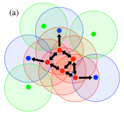
Figure 1: Schematics of DBSCAN. (a) Red, blue, green points are core points, boarder points, and outliers, respectively. Red and blue points form one cluster. These definitions are consistent with setting $n_{\mathrm{min}}$ to any value in the set $\{2,3,4\}$. (b) Red and blue data points form clusters and green data points are outliers. DBSCAN is applicable to linearly nonseparable datasets. These clustering results correspond to setting $n_{\mathrm{min}}$ to any value in the set $\{3,4,\cdots,15\}$.

DBSCAN is usually applied to systems or datasets with the open boundary condition, but the Vicsek model has the periodic boundary condition. With small modification, DBSCAN is applicable to a periodic boundary condition in Ref. [37].

III.2 Cost function of DBSCAN

We first introduce a cost function and show that the DBSCAN algorithm yield solutions that are close to minima of this cost function, and that the DBSCAN algorithm implements an approximate version of a local update rule for minimizing the cost function. We thus establish an optimization basis for DBSCAN.

Let $l_{i}\in\{0,1,\ldots,N_{\mathrm{cl}}\}$ be the label assigned to the $i^{th}$ data point $x_{i}$, where $N_{\mathrm{cl}}$ is an integer sufficiently larger than the actual number of clusters $n_{\mathrm{cl}}$ that DBSCAN would determine or present in the dataset. Also, let $N_{l}$ be the number of data points that have been assigned the label $l$. We then define a free-energy type of cost function:

$$F_{\beta}(\{l_{i}\}_{i=1}^{n_{\mathrm{ag}}}) \coloneqq U_{r_{\mathrm{D}},n_{\mathrm{min}}}(\{l_{i}\}_{i=1}^{n_{\mathrm{ag}}})-\beta S(\{l_{i}\}).$$ (3.1)

The individual terms are then defined as:

$$U_{r_{\mathrm{D}},n_{\mathrm{min}}}(\{l_{i}\}_{i=1}^{n_{\mathrm{ag}}}) \coloneqq-J\sum_{i=1}^{n_{\mathrm{ag}}}\delta_{l_{i},\tilde{l}_{i}(r_{\mathrm{D}},n_{\mathrm{min}})},$$ (3.2)

$$S(\{l_{i}\}) \coloneqq-\bigg{(}\sum_{l=1}^{N_{\mathrm{cl}}}N_{l}\ln N_{l}\bigg{)}+\bigg{(}\sum_{l=1}^{N_{\mathrm{cl}}}N_{l}\bigg{)}\ln\bigg{(}\sum_{l=1}^{N_{\mathrm{cl}}}N_{l}\bigg{)},$$ (3.3)

where

$$\tilde{l}_{i}(r_{\mathrm{D}},n_{\mathrm{min}})$$

$$\quad\coloneqq\begin{dcases}\operatorname*{arg\,max}_{l=1,2,\dots,n_{\mathrm{cl}}}N_{i,l}(r_{\mathrm{D}},n_{\mathrm{min}})&(\exists l\in\{k\}_{k=1}^{n_{\mathrm{ag}}},N_{i,l}(r_{\mathrm{D}},n_{\mathrm{min}})>0),\\ 0&(\text{otherwise}),\end{dcases}$$ (3.4)

and

$$N_{i,l}(r_{\mathrm{D}},n_{\mathrm{min}}) \coloneqq\begin{cases}\tilde{N}_{i,l}(r_{\mathrm{D}})&(\tilde{N}_{i,l}(r_{\mathrm{D}})\geq n_{\mathrm{min}})\\ 0&(\text{otherwise}).\end{cases},$$ (3.5)

$$\tilde{N}_{i,l}(r_{\mathrm{D}}) \coloneqq\sum_{\begin{subarray}{c}j=1,2,\dots,n_{\mathrm{ag}}:\\ \|\bm{x}_{i}-\bm{x}_{j}\|_{\mathrm{F}}\leq r_{\mathrm{D}}\end{subarray}}\delta_{l,l_{j}}.$$ (3.6)

Furthermore, $\beta$ is a small real number $(0<\beta\ll 1$), and $J>0$ is a positive number.

The choice of the cost function in Eq. (3.1) and how it is related to the output of DBSCAN can be understood by explaining each term in it, and how a Monte Carlo optimization method can be applied to minimize the cost function. Given any assignment of $x_{i}$’s to respective labels $l_{i}$’s a local update rule can be designed as follows. First, for each data point $x_{i}$ and any given label $l$ we evaluate Eq.(3.6) to get the number of data points within radius $r_{\mathrm{D}}$ from the $i$-th datapoint that also have the label $l$. Then, Eq. (3.5) is used to discard the information of labels that do not satisfy the minimum number of datapoints in a cluster $n_{\mathrm{min}}$. Then, we conduct the majority voting with respect to labels by Eq. (3.4): that is, for each $x_{i}$ we find the label $\tilde{l}_{i}(r_{\mathrm{D}},n_{\mathrm{min}})$ that has the maximum number of points assigned to it. Finally, we update the label assignments by minimizing Eq. (3.2) under the constraint of Eq. (3.3). A greedy strategy could be to assign the majority label as the new label of a datapoint. However, without Eq. (3.3), the number of clusters is more likely to be underestimated; thus Eq. (3.3) is necessary. For instance, even when dealing with two well-separated clusters, combining them into a single cluster yields the same value for Eq. (3.2).

Returning to DBSCAN, the first and the dominant term of the cost function in Eq. (3.2), favors the same label of a node as obtained by a majority voting, as computed in Eq. (3.4). In this sense, the minimization of Eq. (3.1) and DBSCAN have locally almost the same dynamics. Moreover, since DBSCAN provides a method for starting a new cluster label when a new core node is encountered, it automatically incorporates the constraint in Eq. (3.3). Thus, any labeling assignment obtained by DBSCAN is already very close to a local minimum of the cost function. That is, performing local updates for our cost function starting from a DBSCAN label assignment would keep it mostly unchanged.

III.3 Why DBSCAN

We have chosen DBSCAN to analyze the cluster phases of the Vicsek model although there have been many clustering algorithms proposed in the literature [25]. The simplest explanation is that its cost function, Eq. (3.1), shares similarities with the cost function of the Vicsek model, Eq. (2.9). As mentioned in Ref. [1], the Vicsek model becomes the random $XY$ model, in which agents interact with radius $r_{\mathrm{V}}$, in the limit $v_{\mathrm{abs}}\to 0$. As shown in Eq. (3.1), datapoints within radius $r_{\mathrm{V}}$ also interact in DBSCAN. Then, the cost function of DBSCAN can be seen as a discretized version of the cost function of the Vicsek model. The continuous state variables $\theta_{i}$’s in the Vicsek model are replaced by the discrete label assignments $l_{i}$’s in DBSCAN. Moreover in equation 2.9, instead of taking the average of $\theta_{i}$’s in a neighborhood $r_{\mathrm{V}}$, the majority of the labels of the datapoints in a neighborhood $r_{\mathrm{V}}$ is computed. With these substitutions, the first term in Eq.3.2 is almost identical to 2.9. Because the state variables are discrete in the DBSCAN formulation, the term Eq. (3.3) is necessary to prevent mode collapse. However, their dynamical behaviors are different: the dynamics of DBSCAN is described by a greedy algorithm (where only randomness is in the order in which datapoints are visited), while the dynamics of the Vicsek model is a stochastic process. Additionally, in the case of the Vicsek model, each agent moves at a constant speed $v_{\mathrm{abs}}$; by taking the limit of $v_{\mathrm{abs}}\to 0$, their dynamical behaviors become more similar.

III.4 Definition of new order parameters

Introducing two parameters $\alpha$ and $\beta$ as new order parameters, we consider the following relationship between $n_{\mathrm{ag}}$ and $n_{\mathrm{cl}}$:

$$n_{\mathrm{cl}} =\alpha+\beta n_{\mathrm{ag}}.$$ (3.7)

Note that numerical simulations shown later indicates that $\alpha\in[0,1]$ and $\beta\geq 0$. In the section of numerics, we will observe the following ”phase transitions”:

$$(\alpha=0,\beta=0) \Leftrightarrow(\alpha=0,\beta>0),$$ (3.8)

$$(\alpha=0,\beta>0) \Leftrightarrow(\alpha=1,\beta=0).$$ (3.9)

We also see, via numerical simulations, that the phase of $(\alpha=1,\beta>0)$ does not exist.

IV Numerical simulations

In Fig. 2, we plot the dependence of $n_{\mathrm{cl}}$ and $v_{\mathrm{op}}(t)$ on $r_{\mathrm{V}}$ and $\eta$ for the Vicsek model with metric interaction. We set $r_{\mathrm{V}}=r_{\mathrm{D}}$, $n_{\mathrm{ag}}=400$, $L=10.0$, $\Delta t=1.0$, $v_{\mathrm{abs}}=0.030$, $n_{\mathrm{min}}=5$, and $t=100$. We repeated the same calculations 10 times to compute the statistical means. Here after we write the number of repetition $n_{\mathrm{rep}}$.

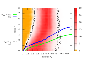
Figure 2: Dependence of $n_{\mathrm{cl}}$ (heat map) and $v_{\mathrm{op}}(t)$ (solid lines) on $r_{\mathrm{V}}$ (horizontal) and $\eta$ (vertical) for the Vicsek model with the metric interaction. We set $r_{\mathrm{V}}=r_{\mathrm{D}}$, $n_{\mathrm{ag}}=400$, $L=10.0$, $\Delta t=1.0$, $v_{\mathrm{abs}}=0.030$, $n_{\mathrm{min}}=5$, $t=100$, and $n_{\mathrm{rep}}=10$. The black dotted and dashed lines are contour lines for the number of estimated number of clusters.

Figure 2 implies that the number of clusters $n_{\mathrm{cl}}$ exhibits phase transitions or crossovers twice upon increasing $r_{\mathrm{V}}$ with fixed $\eta$: from the orange regime to the red regime, and from the red regime to the white regime. By combining the order parameter proposed in Ref.[1], Eq. (2.10), with $n_{\mathrm{cl}}$, we identify at least five regimes, as the red and white regimes are each divided into two in addition to the orange regime.

To examine the robustness of the phases shown in Fig. 2 with respect to $n_{\mathrm{min}}$, we plot the dependence of $n_{\mathrm{cl}}$ and $v_{\mathrm{op}}(t)$ on $r_{\mathrm{V}}$ and $\eta$ for the Vicsek model with the metric interaction when $n_{\mathrm{min}}=1$ in Fig. 3. We use the same parameter values as in Fig. 2 for all other parameters.

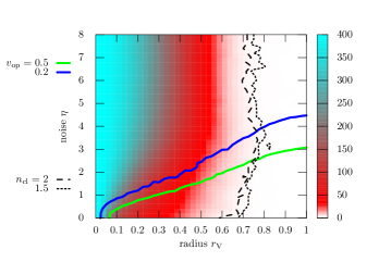
Figure 3: Dependence of $n_{\mathrm{cl}}$ (heat map) and $v_{\mathrm{op}}(t)$ (lines) on $r_{\mathrm{V}}$ (horizontal) and $\eta$ (vertical) for the Vicsek model with the metric interaction. We set $r_{\mathrm{V}}=r_{\mathrm{D}}$, $n_{\mathrm{ag}}=400$, $L=10.0$, $\Delta t=1.0$, $v_{\mathrm{abs}}=0.030$, $n_{\mathrm{min}}=1$, $t=100$, and $n_{\mathrm{rep}}=10$. The black dotted and dashed lines are contour lines for the number of estimated number of clusters.

The colorbars of Fig. 3 and 2 are identical from 0 to 35. The main difference between the two figures is the orange regime in Fig. 2 and the cyan regime in Fig. 3. This is because, in this regime, all the agents move almost randomly due to small $r_{\mathrm{V}}$ and large $\eta$. In Fig. 2, no clusters are found because of $n_{\mathrm{min}}=5$, resulting in $n_{\mathrm{cl}}=0$, whereas in Fig. 3, all the agents are considered as clusters because of $n_{\mathrm{min}}=1$, resulting in $n_{\mathrm{cl}}=400$. Moreover, the red and white regimes in both figures are the same, regardless of the difference in $n_{\mathrm{min}}$.

So far, we have discussed the phases for fixed $n_{\mathrm{ag}}$, but it is important to understand the behavior of the phases for large $n_{\mathrm{ag}}$, as we are interested in the thermodynamic limit. In Fig. 4, we plot the dependence of $n_{\mathrm{cl}}$ on $n_{\mathrm{ag}}$ for the Vicsek model with metric interaction. We set $r_{\mathrm{V}}=r_{\mathrm{D}}=0.40$, $\eta=4.0$, $L=10.0$, $\Delta t=1.0$, $v_{\mathrm{abs}}=0.030$, $n_{\mathrm{min}}=5$, $t=100$, and $n_{\mathrm{rep}}=10$. We vary $L$ such that $n_{\mathrm{ag}}/L^{2}=400/10.0^{2}$, i.e., we use parameters that belong to the red regime of Fig. 2 and Fig. 3.

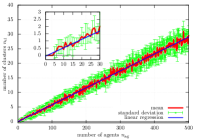
Figure 4: Dependence of $n_{\mathrm{cl}}$ on $n_{\mathrm{ag}}$ for the Vicsek model with the metric interaction. We set $r_{\mathrm{V}}=r_{\mathrm{D}}=0.40$, $\eta=4.0$, $L=10.0$, $\Delta t=1.0$, $v_{\mathrm{abs}}=0.030$, $n_{\mathrm{min}}=5$, $t=100$, and $n_{\mathrm{rep}}=10$. We vary $L$ such that $n_{\mathrm{ag}}/L^{2}=400/10.0^{2}$. The linear regression function is $f(x)=0.0581236x-0.0630702$. We used the data in the range of $n_{\mathrm{ag}}\in[10,500]$ to estimate the linear regression function.

Figure 4 clearly shows a linear relationship between $n_{\mathrm{ag}}$ and $n_{\mathrm{cl}}$, crossing the origin. We also plot the linear regression function: $f(x)=0.0581236x-0.0630702$. We used the data in the range of $n_{\mathrm{ag}}in[10,500]$ to estimate this linear regression function. Note that for small values of $n_{\mathrm{ag}}$, the estimate of $n_{\mathrm{cl}}$ may not be reliable because of the discreteness affecting the estimates. This estimated linear regression function supports that $\alpha=0$ and $\beta>0$, where $\alpha$ and $\beta$ are defined in Eq. (3.7).

In Fig. 5, we also show the dependence of $n_{\mathrm{cl}}$ on $n_{\mathrm{ag}}$ for the Vicsek model with the metric interaction in the case of $r_{\mathrm{V}}=r_{\mathrm{D}}=1.0$. We use the same values with Fig. 4 for the other parameters. That is, we use parameters that belong to the white regime of Fig. 2 and Fig. 3.

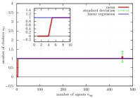
Figure 5: Dependence of $n_{\mathrm{cl}}$ on $n_{\mathrm{ag}}$ for the Vicsek model with the metric interaction. We set $r_{\mathrm{V}}=r_{\mathrm{D}}=1.0$, $\eta=4.0$, $L=10.0$, $\Delta t=1.0$, $v_{\mathrm{abs}}=0.030$, $n_{\mathrm{min}}=5$, $t=100$, and $n_{\mathrm{rep}}=10$. We vary $L$ such that $n_{\mathrm{ag}}/L^{2}=400/10.0^{2}$. The linear regression function is $f(x)=4.06521\times 10^{-6}x+0.999371$. We used the data in the range of $n_{\mathrm{ag}}\in[10,500]$ to estimate the linear regression function.

Figure 4 also clearly shows that $n_{\mathrm{cl}}=1$ independently of $n_{\mathrm{ag}}$. The linear regression function is $f(x)=4.06521\times 10^{-6}x+0.999371$. We used the data in the range of $n_{\mathrm{ag}}\in[10,500]$ to estimate the linear regression function. This estimated linear regression function implies that $\alpha=1$ and $\beta=0$ for $\alpha$ and $\beta$ defined in Eq. (3.7). Thus, we can see the discontinuous transition of $\alpha$ across the red and white regimes of Fig. 2 and Fig. 3.

V Discussions

In Fig. 6, we present the schematic of the phase of the Vicsek model. Therein we define new symbols: (A1) non-Vicsek-ordered state with no clusters, (A2, A2’) non-Vicsek-ordered state with multiple clusters, (A3) non-Vicsek-ordered state with one cluster, (B1) Vicsek-ordered state with no clusters, (B2) Vicsek-ordered state with multiple clusters, and (B3) Vicsek-ordered state with one cluster .

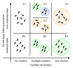
Figure 6: Schematic of the phases of the Vicsek model: (A1) non-Vicsek-ordered state with no clusters, (A2, A2’) non-Vicsek-ordered state with multiple clusters, (A3) non-Vicsek-ordered state with one cluster, (B1) Vicsek-ordered state with no clusters, (B2) Vicsek-ordered state with multiple clusters, and (B3) Vicsek-ordered state with one cluster. The difference between phase A2 and phase A2’ is whether agents within clusters are Vicsek-ordered or not.

In Fig. 2, either phase A2 or phase A2’ is expected to occur in the regime of $\eta\geq 3.0$ and $r_{\mathrm{V}}\in[0.3,0.5]$. To identify the phase, in addition to $v_{\mathrm{op}}(t)$ in Eq. (2.10), we also define the following clusterwise order parameters for $j=1,2,\dots,n_{\mathrm{cl}}$:

$$v_{\mathrm{op}}^{(j)}(t) \coloneqq\frac{1}{v_{\mathrm{abs}}|C_{j}|}\bigg{\|}\sum_{i\in C_{j}}\bm{v}_{i}(t)\bigg{\|}_{\mathrm{F}},$$ (5.1)

where $C_{j}$ is the set of labels that belong to cluster $j$. In Fig. 7, we plot the time dependence of $v_{\mathrm{op}}(t)$ in Eq. (2.10) and $v_{\mathrm{op}}^{(j)}(t)$ in Eq. (5.1) for $j=1,2,3$ in the case of $r_{\mathrm{V}}=r_{\mathrm{D}}=0.40$, $n_{\mathrm{ag}}=400$, $\eta=4.0$, $L=10.0$, $\Delta t=1.0$, $v_{\mathrm{abs}}=0.030$, and $n_{\mathrm{min}}=5$. Note that the chosen parameter set corresponds to the regime in which the system exhibits non-Vicsek-ordered states with multiple clusters. We computed the time averages of $v_{\mathrm{op}}^{(j)}(t)$ and $v_{\mathrm{op}}(t)$ using data in the range $t\in[10,100]$ and plotted them. The clusters were randomly selected, although the total number of clusters $n_{\mathrm{cl}}$ is much greater than three.

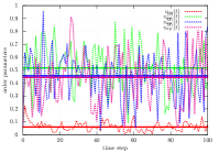
Figure 7: (dashed lines) Time depednece of $v_{\mathrm{op}}(t)$ and $v_{\mathrm{op}}^{(j)}(t)$ for $j=1,2,3$. We set $r_{\mathrm{V}}=r_{\mathrm{D}}=0.40$, $n_{\mathrm{ag}}=400$, $\eta=4.0$, $L=10.0$, $\Delta t=1.0$, $v_{\mathrm{abs}}=0.030$, and $n_{\mathrm{min}}=5$. (solid lines) We also draw the time averages of $v_{\mathrm{op}}(t)$ and $v_{\mathrm{op}}^{(j)}(t)$ for $j=1,2,3$. We used the data in the range of $[10,100]$ to compute the time averages.

First, $v_{\mathrm{op}}(t)$ is very small as the parameter set in the regime of non-Vicsek-ordered states. However, $v_{\mathrm{op}}^{(j)}(t)$ is much larger for $j=1,2,3$. This result implies that agents are not Vicsek-ordered from the macroscopic viewpoint, but Vicsek-ordered within clusters. Note that cluster labels may not be consistent because clusters often merge or split during the dynamics of the Vicsek model and the results shown in Fig. 7 represent one realization.

In Fig. 8, we added the labels (A1, A2, A2’, A3, B1, B2, B3) defined in Fig. 6 to Fig. 2.

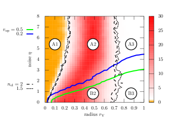
Figure 8: Phase diagram of the Vicsek model with the labels of phases. The numerical setup is the same with Fig. 2 and the labels of the phases are defined in Fig. 6.

First, phase B1 does not exist in the phase diagram simply because $v_{\mathrm{op}}(t)$ in Eq. (2.10) cannot be nonzero without a global cluster or local clusters. Second, Fig. 7 implies that phase A2’ also does not exist in the phase diagram. Finally, the existence of phase A1 depends on $n_{\mathrm{min}}$ in DBSCAN as shown in Fig. 3.

VI Conclusions

In this paper, we investigate the cluster dynamics of the Vicsek model. We first examine the relationship between the Vicsek model and DBSCAN, focusing on their cost functions. We use DBSCAN, a widely used machine learning algorithm, to estimate the cluster structure of the Vicsek model. Our findings are important for two reasons. Firstly, we identify new phases in the well-known Vicsek model, which has significant implications for natural science. Secondly, we discover a mathematical relationship between the Vicsek model and DBSCAN. A cost function of DBSCAN was not explicitly defined in the original paper, so this relationship was not previously understood. Our work bridges two different fields and opens up new directions for research by combining them.

Appendix A Additional numerical simulations (phase diagrams)

In Fig. 9, we plot the dependence of $n_{\mathrm{cl}}$ and $v_{\mathrm{op}}(t)$ on $r_{\mathrm{V}}$ and $\eta$ for the Vicsek model with metric interaction. We set $r_{\mathrm{V}}=r_{\mathrm{D}}$, $n_{\mathrm{ag}}=400$, $L=10.0$, $\Delta t=1.0$, $v_{\mathrm{abs}}=0.030$, $n_{\mathrm{min}}=3$, and $t=100$. We repeated the same calculations 10 times to compute the statistical means. Here after we write the number of repetition $n_{\mathrm{rep}}$.

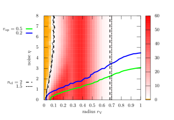
Figure 9: Dependence of $n_{\mathrm{cl}}$ (heat map) and $v_{\mathrm{op}}(t)$ (solid lines) on $r_{\mathrm{V}}$ (horizontal) and $\eta$ (vertical) for the Vicsek model with the metric interaction. We set $r_{\mathrm{V}}=r_{\mathrm{D}}$, $n_{\mathrm{ag}}=400$, $L=10.0$, $\Delta t=1.0$, $v_{\mathrm{abs}}=0.030$, $n_{\mathrm{min}}=3$, $t=100$, and $n_{\mathrm{rep}}=10$. The black dotted and dashed lines are contour lines for the number of estimated number of clusters.

In Fig. 10, we plot the dependence of $n_{\mathrm{cl}}$ and $v_{\mathrm{op}}(t)$ on $r_{\mathrm{V}}$ and $\eta$ for the Vicsek model with metric interaction. We set $r_{\mathrm{V}}=r_{\mathrm{D}}$, $n_{\mathrm{ag}}=400$, $L=10.0$, $\Delta t=1.0$, $v_{\mathrm{abs}}=0.030$, $n_{\mathrm{min}}=7$, and $t=100$. We repeated the same calculations 10 times to compute the statistical means. Here after we write the number of repetition $n_{\mathrm{rep}}$.

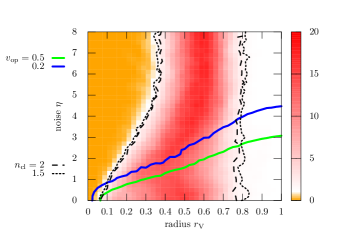
Figure 10: Dependence of $n_{\mathrm{cl}}$ (heat map) and $v_{\mathrm{op}}(t)$ (solid lines) on $r_{\mathrm{V}}$ (horizontal) and $\eta$ (vertical) for the Vicsek model with the metric interaction. We set $r_{\mathrm{V}}=r_{\mathrm{D}}$, $n_{\mathrm{ag}}=400$, $L=10.0$, $\Delta t=1.0$, $v_{\mathrm{abs}}=0.030$, $n_{\mathrm{min}}=7$, $t=100$, and $n_{\mathrm{rep}}=10$. The black dotted and dashed lines are contour lines for the number of estimated number of clusters.

In Fig. 11, we plot the dependence of $n_{\mathrm{cl}}$ and $v_{\mathrm{op}}(t)$ on $r_{\mathrm{V}}$ and $\eta$ for the Vicsek model with metric interaction. We set $r_{\mathrm{V}}=r_{\mathrm{D}}$, $n_{\mathrm{ag}}=400$, $L=10.0$, $\Delta t=1.0$, $v_{\mathrm{abs}}=0.030$, $n_{\mathrm{min}}=10$, and $t=100$. We repeated the same calculations 10 times to compute the statistical means. Here after we write the number of repetition $n_{\mathrm{rep}}$.

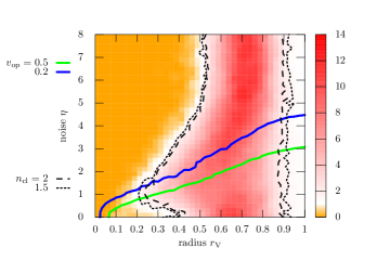
Figure 11: Dependence of $n_{\mathrm{cl}}$ (heat map) and $v_{\mathrm{op}}(t)$ (solid lines) on $r_{\mathrm{V}}$ (horizontal) and $\eta$ (vertical) for the Vicsek model with the metric interaction. We set $r_{\mathrm{V}}=r_{\mathrm{D}}$, $n_{\mathrm{ag}}=400$, $L=10.0$, $\Delta t=1.0$, $v_{\mathrm{abs}}=0.030$, $n_{\mathrm{min}}=10$, $t=100$, and $n_{\mathrm{rep}}=10$. The black dotted and dashed lines are contour lines for the number of estimated number of clusters.

Appendix B Additional numerical simulations (system size dependence)

We show additional numerical simulations on the dependence of $n_{\mathrm{cl}}$ on $n_{\mathrm{ag}}$ for the Vicsek model with metric interaction near the boundary between $(\alpha=0,\beta>0)$ and $(\alpha=1.0,\beta=0)$.

In Fig. 12, we plot the dependence of $n_{\mathrm{cl}}$ on $n_{\mathrm{ag}}$ for the Vicsek model with metric interaction. We set $r_{\mathrm{V}}=r_{\mathrm{D}}=0.6$, $\eta=4.0$, $L=10.0$, $D=2$, $\Delta t=1.0$, $v_{\mathrm{abs}}=0.030$, $n_{\mathrm{rep}}=10$, $n_{\mathrm{min}}=5$, and $t=100$. We vary $L$ such that $n_{\mathrm{ag}}/L^{2}=400/10.0^{2}$.

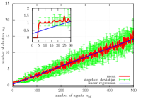
Figure 12: Dependence of $n_{\mathrm{cl}}$ on $n_{\mathrm{ag}}$ for the Vicsek model with the metric interaction. We set $r_{\mathrm{V}}=r_{\mathrm{D}}=0.6$, $\eta=4.0$, $L=10.0$, $D=2$, $\Delta t=1.0$, $v_{\mathrm{abs}}=0.030$, $n_{\mathrm{rep}}=10$, $n_{\mathrm{min}}=5$, and $t=100$. We vary $L$ such that $n_{\mathrm{ag}}/L^{2}=400/10.0^{2}$. The linear regression function is $f(x)=0.0277741x+0.289242$. We used the data in regime of $n)\mathrm{ag}\in[10,500]$ to estimate the linear regression function.

In this setup, $n_{\mathrm{cl}}$ increases linearly with $n_{\mathrm{ag}}$ though $n_{\mathrm{cl}}$ shows a step function-like behavior on $n_{\mathrm{ag}}$ for small $n_{\mathrm{ag}}$.

In Fig. 13, we plot the dependence of $n_{\mathrm{cl}}$ on $n_{\mathrm{ag}}$ for the Vicsek model with metric interaction. We set $r_{\mathrm{V}}=r_{\mathrm{D}}=0.7$, $\eta=4.0$, $L=10.0$, $D=2$, $\Delta t=1.0$, $v_{\mathrm{abs}}=0.030$, $n_{\mathrm{rep}}=10$, $n_{\mathrm{min}}=5$, and $t=100$. We vary $L$ such that $n_{\mathrm{ag}}/L^{2}=400/10.0^{2}$.

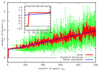
Figure 13: Dependence of $n_{\mathrm{cl}}$ on $n_{\mathrm{ag}}$ for the Vicsek model with the metric interaction. We set $r_{\mathrm{V}}=r_{\mathrm{D}}=0.7$, $\eta=4.0$, $L=10.0$, $D=2$, $\Delta t=1.0$, $v_{\mathrm{abs}}=0.030$, $n_{\mathrm{rep}}=10$, $n_{\mathrm{min}}=5$, and $t=100$. We vary $L$ such that $n_{\mathrm{ag}}/L^{2}=400/10.0^{2}$. The linear regression function is $f(x)=0.00421017x+0.832924$. We used the data in the regime of $n_{\mathrm{ag}}\in[10,500]$ to estimate the linear regression function.

In this setup, $(\alpha\approx 1.0,\beta>0)$ is realized. However, this parameter regime is quite small. Further investigation is necessary to verify the robustness of this phase in the thermodynamic limit.

Appendix C Additional numerical simulations (system size dependence) (cont’d)

In Fig. 14, we plot the dependence of $n_{\mathrm{cl}}$ on $n_{\mathrm{ag}}$ for the Vicsek model with metric interaction. We set $r_{\mathrm{V}}=r_{\mathrm{D}}=0.5$, $\eta=4.0$, $L=10.0$, $D=2$, $\Delta t=1.0$, $v_{\mathrm{abs}}=0.030$, $n_{\mathrm{rep}}=10$, $n_{\mathrm{min}}=5$, and $t=100$. We vary $L$ such that $n_{\mathrm{ag}}/L^{2}=400/10.0^{2}$.

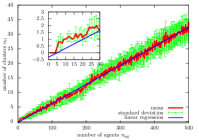
Figure 14: Dependence of $n_{\mathrm{cl}}$ on $n_{\mathrm{ag}}$ for the Vicsek model with the metric interaction. We set $r_{\mathrm{V}}=r_{\mathrm{D}}=0.5$, $\eta=4.0$, $L=10.0$, $D=2$, $\Delta t=1.0$, $v_{\mathrm{abs}}=0.030$, $n_{\mathrm{rep}}=10$, $n_{\mathrm{min}}=5$, and $t=100$. We vary $L$ such that $n_{\mathrm{ag}}/L^{2}=400/10.0^{2}$. The linear regression function is $f(x)=0.0652563x-0.324467$. We used the data in regime of $n)\mathrm{ag}\in[10,500]$ to estimate the linear regression function.

In Fig. 15, we plot the dependence of $n_{\mathrm{cl}}$ on $n_{\mathrm{ag}}$ for the Vicsek model with metric interaction. We set $r_{\mathrm{V}}=r_{\mathrm{D}}=0.8$, $\eta=4.0$, $L=10.0$, $D=2$, $\Delta t=1.0$, $v_{\mathrm{abs}}=0.030$, $n_{\mathrm{rep}}=10$, $n_{\mathrm{min}}=5$, and $t=100$. We vary $L$ such that $n_{\mathrm{ag}}/L^{2}=400/10.0^{2}$.

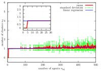
Figure 15: Dependence of $n_{\mathrm{cl}}$ on $n_{\mathrm{ag}}$ for the Vicsek model with the metric interaction. We set $r_{\mathrm{V}}=r_{\mathrm{D}}=0.8$, $\eta=4.0$, $L=10.0$, $D=2$, $\Delta t=1.0$, $v_{\mathrm{abs}}=0.030$, $n_{\mathrm{rep}}=10$, $n_{\mathrm{min}}=5$, and $t=100$. We vary $L$ such that $n_{\mathrm{ag}}/L^{2}=400/10.0^{2}$. The linear regression function is $f(x)=0.00040936x+0.971784$. We used the data in regime of $n)\mathrm{ag}\in[10,500]$ to estimate the linear regression function.

In Fig. 16, we plot the dependence of $n_{\mathrm{cl}}$ on $n_{\mathrm{ag}}$ for the Vicsek model with metric interaction. We set $r_{\mathrm{V}}=r_{\mathrm{D}}=0.9$, $\eta=4.0$, $L=10.0$, $D=2$, $\Delta t=1.0$, $v_{\mathrm{abs}}=0.030$, $n_{\mathrm{rep}}=10$, $n_{\mathrm{min}}=5$, and $t=100$. We vary $L$ such that $n_{\mathrm{ag}}/L^{2}=400/10.0^{2}$.

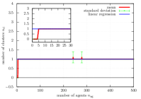
Figure 16: Dependence of $n_{\mathrm{cl}}$ on $n_{\mathrm{ag}}$ for the Vicsek model with the metric interaction. We set $r_{\mathrm{V}}=r_{\mathrm{D}}=0.9$, $\eta=4.0$, $L=10.0$, $D=2$, $\Delta t=1.0$, $v_{\mathrm{abs}}=0.030$, $n_{\mathrm{rep}}=10$, $n_{\mathrm{min}}=5$, and $t=100$. We vary $L$ such that $n_{\mathrm{ag}}/L^{2}=400/10.0^{2}$. The linear regression function is $f(x)=9.12391\times 10^{-08}x+1.00038$. We used the data in regime of $n)\mathrm{ag}\in[10,500]$ to estimate the linear regression function.

References

- Vicsek et al. [1995] T. Vicsek, A. Czirók, E. Ben-Jacob, I. Cohen, and O. Shochet, Novel type of phase transition in a system of self-driven particles, Phys. Rev. Lett. 75, 1226 (1995).
- Cavagna and Giardina [2014] A. Cavagna and I. Giardina, Bird flocks as condensed matter, Annual Review of Condensed Matter Physics 5, 183 (2014).
- Cavagna et al. [2015] A. Cavagna, L. Del Castello, I. Giardina, T. Grigera, A. Jelic, S. Melillo, T. Mora, L. Parisi, E. Silvestri, M. Viale, et al., Flocking and turning: a new model for self-organized collective motion, Journal of Statistical Physics 158, 601 (2015).
- Ramaswamy [2010] S. Ramaswamy, The mechanics and statistics of active matter, Annual Review of Condensed Matter Physics 1, 323 (2010).
- Parrish [1997] J. K. Parrish, ed., Animal Groups in Three Dimensions: How Species Aggregate (Cambridge University Press, 1997).
- Bonner [1998] J. T. Bonner, A way of following individual cells in the migrating slugs of ¡i¿dictyostelium discoideum¡/i¿, Proceedings of the National Academy of Sciences 95, 9355 (1998), https://www.pnas.org/doi/pdf/10.1073/pnas.95.16.9355 .
- Harada et al. [1987] Y. Harada, A. Noguchi, A. Kishino, and T. Yanagida, Sliding movement of single actin filaments on one-headed myosin filaments, Nature 326, 805 (1987).
- Angelini et al. [2011] T. E. Angelini, E. Hannezo, X. Trepat, M. Marquez, J. J. Fredberg, and D. A. Weitz, Glass-like dynamics of collective cell migration, Proceedings of the National Academy of Sciences 108, 4714 (2011), https://www.pnas.org/doi/pdf/10.1073/pnas.1010059108 .
- Helbing et al. [2000] D. Helbing, I. Farkas, and T. Vicsek, Simulating dynamical features of escape panic, Nature 407, 487 (2000).
- Keta et al. [2021] Y.-E. Keta, E. Fodor, F. van Wijland, M. E. Cates, and R. L. Jack, Collective motion in large deviations of active particles, Phys. Rev. E 103, 022603 (2021).
- Keta et al. [2022] Y.-E. Keta, R. L. Jack, and L. Berthier, Disordered collective motion in dense assemblies of persistent particles, Phys. Rev. Lett. 129, 048002 (2022).
- Fruchart et al. [2021] M. Fruchart, R. Hanai, P. B. Littlewood, and V. Vitelli, Non-reciprocal phase transitions, Nature 592, 363 (2021).
- Hanai and Littlewood [2020] R. Hanai and P. B. Littlewood, Critical fluctuations at a many-body exceptional point, Physical Review Research 2, 033018 (2020).
- Bertin et al. [2006] E. Bertin, M. Droz, and G. Grégoire, Boltzmann and hydrodynamic description for self-propelled particles, Phys. Rev. E 74, 022101 (2006).
- Bertin et al. [2009] E. Bertin, M. Droz, and G. Grégoire, Hydrodynamic equations for self-propelled particles: microscopic derivation and stability analysis, Journal of Physics A: Mathematical and Theoretical 42, 445001 (2009).
- Marchetti et al. [2013] M. C. Marchetti, J. F. Joanny, S. Ramaswamy, T. B. Liverpool, J. Prost, M. Rao, and R. A. Simha, Hydrodynamics of soft active matter, Rev. Mod. Phys. 85, 1143 (2013).
- Ãtienne Fodor and Cristina Marchetti [2018] Ãtienne Fodor and M. Cristina Marchetti, The statistical physics of active matter: From self-catalytic colloids to living cells, Physica A: Statistical Mechanics and its Applications 504, 106 (2018), lecture Notes of the 14th International Summer School on Fundamental Problems in Statistical Physics.
- Shankar et al. [2020] S. Shankar, A. Souslov, M. J. Bowick, M. C. Marchetti, and V. Vitelli, Topological active matter, arXiv preprint arXiv:2010.00364 (2020).
- Carleo et al. [2019] G. Carleo, I. Cirac, K. Cranmer, L. Daudet, M. Schuld, N. Tishby, L. Vogt-Maranto, and L. Zdeborová, Machine learning and the physical sciences, Rev. Mod. Phys. 91, 045002 (2019).
- Das Sarma et al. [2019] S. Das Sarma, D.-L. Deng, and L.-M. Duan, Machine learning meets quantum physics, Physics Today 72, 48 (2019).
- Guo et al. [2020] W.-c. Guo, B.-q. Ai, and L. He, Reveal flocking of birds flying in fog by machine learning, arXiv preprint arXiv:2005.10505 (2020).
- Chen and Qiu [2020] X. Chen and Y. Qiu, An effective multi-level synchronization clustering method based on a linear weighted vicsek model, Applied Intelligence 50, 4063 (2020).
- de Koning [2020] M. de Koning, Machine learning phases of active matter: Finite size scaling in the vicsek model by means of a principle component analysis and neural networks (2020).
- Bhaskar et al. [2019] D. Bhaskar, A. Manhart, J. Milzman, J. T. Nardini, K. M. Storey, C. M. Topaz, and L. Ziegelmeier, Analyzing collective motion with machine learning and topology, Chaos: An Interdisciplinary Journal of Nonlinear Science 29, 123125 (2019).
- [25] scikit learn, Clustering.
- Bishop [2006] C. M. Bishop, Pattern recognition and machine learning (springer, 2006).
- Murphy [2012] K. P. Murphy, Machine learning: a probabilistic perspective (MIT press, 2012).
- Ankerst et al. [1999] M. Ankerst, M. M. Breunig, H.-P. Kriegel, and J. Sander, Optics: Ordering points to identify the clustering structure, ACM Sigmod record 28, 49 (1999).
- Ester et al. [1996] M. Ester, H.-P. Kriegel, J. Sander, X. Xu, et al., A density-based algorithm for discovering clusters in large spatial databases with noise., in kdd, Vol. 96 (1996) pp. 226–231.
- López [2004] C. López, Clustering transition in a system of particles self-consistently driven by a shear flow, Phys. Rev. E 70, 066205 (2004).
- Ginot et al. [2018] F. Ginot, I. Theurkauff, F. Detcheverry, C. Ybert, and C. Cottin-Bizonne, Aggregation-fragmentation and individual dynamics of active clusters, Nature communications 9, 696 (2018).
- Ferdinandy et al. [2017] B. Ferdinandy, K. Ozogány, and T. Vicsek, Collective motion of groups of self-propelled particles following interacting leaders, Physica A: Statistical Mechanics and its Applications 479, 467 (2017).
- Schubert et al. [2017] E. Schubert, J. Sander, M. Ester, H. P. Kriegel, and X. Xu, Dbscan revisited, revisited: Why and how you should (still) use dbscan, ACM Trans. Database Syst. 42, 10.1145/3068335 (2017).
- Gao [2013] J. Gao, Data mining and bioinformatics (2013).
- Kang et al. [2018] C.-P. Kang, H.-C. Tu, T.-F. Fu, J.-M. Wu, P.-H. Chu, and D. T.-H. Chang, An automatic method to calculate heart rate from zebrafish larval cardiac videos, BMC bioinformatics 19, 1 (2018).
- Harris [2015] N. Harris, Visualizing dbscan clustering (2015).
- [37] F. Turci, Clustering and periodic boundaries.