Functional Slicing-free Inverse Regression via Martingale Difference Divergence Operator

Abstract:  Functional sliced inverse regression (FSIR) is one of the most popular algorithms for functional sufficient dimension reduction (FSDR). However, the choice of slice scheme in FSIR is critical but challenging. In this paper, we propose a new method called functional slicing-free inverse regression (FSFIR) to estimate the central subspace in FSDR. FSFIR is based on the martingale difference divergence operator, which is a novel metric introduced to characterize the conditional mean independence of a functional predictor on a multivariate response. We also provide a specific convergence rate for the FSFIR estimator. Compared with existing functional sliced inverse regression methods, FSFIR does not require the selection of a slice number. Simulations demonstrate the efficiency and convenience of FSFIR.

Key words and phrases: Functional sliced inverse regression, Functional slicing-free inverse regression, Martingale difference divergence, Sufficient dimension reduction.

1 Introduction

Classical statistical methods often failed in the high-dimensional data where the number of features $p$ is comparable to or even larger than the number of observed samples $n$. Sufficient dimension reduction (SDR) is often the first step in dealing with high-dimensional problems. SDR aims to finding the minimal low-rank projection, of a predictor $\boldsymbol{X}\in\mathbb{R}^{p}$, which contains all the information of a response $Y\in\mathbb{R}$ without estimating the unknown link function. Indeed, SDR gives the intersection of all spaces $\mathcal{S}\subset\mathbb{R}^{p}$ satisfying $Y\perp\!\!\!\perp\boldsymbol{X}|P_{\mathcal{S}}\boldsymbol{X}$ where $\perp\!\!\!\perp$ denotes independence and $P_{\mathcal{S}}$ denotes the projection onto $\mathcal{S}$. The said intersection is known as the central subspace and denoted by $\mathcal{S}_{Y|\boldsymbol{X}}$.

There are various well-known SDR methods: sliced inverse regression (SIR, Li 1991), sliced average variance estimation (SAVE, Cook and Weisberg 1991), principal hessian directions (PHD, Li 1992), directional regression (DR, Li and Wang (2007)), minimum average variance estimation (MAVE, Xia et al. (2009)) and many others. Among these methods that deal with the SDR problems, SIR is particularly popular due to its simplicity and efficiency. Under linearity and coverage conditions (See Assumption 2), SIR relates the central subspace $\mathcal{S}_{Y|\boldsymbol{X}}$ with the eigen-space of the covariance of conditional mean, i.e., $\mathrm{var}\left(\mathbb{E}[\boldsymbol{X}|Y]\right)$. Then SIR estimates $\mathrm{var}\left(\mathbb{E}[\boldsymbol{X}|Y]\right)$ by dividing the samples into several equally-sized slices according to the order statistics of response and averaging the sample covariance within each slice.

However, the consistency and convergence rate of SIR, together with other slice-based SDR methods, involve the choice of a suitable slice number (denoted by $H$). Hsing and Carroll (1992) proved that SIR gives a root $n$ consistent estimation when each slice contains two observations (i.e., $H=n/2$), whereas Zhu and Ng (1995) argued that a smaller number of observations in each slice could yield a bigger covariance matrix of asymptotically multinormal distribution of estimators. In addition, by considering the case where the number of samples in each slice, denoted by $c$, goes to infinity with increasing sample size $n$, Zhu and Ng (1995) showed that the optimal $c$ satisfies $c=c_{0}n^{\alpha}$ where $c_{0}>0$ is a constant and $\alpha\in\left(0,1/2\right)$ depends on the distribution of the predictor $\boldsymbol{X}$ and the central curve $m(y):=\mathbb{E}[\boldsymbol{X}|Y=y]$. Nevertheless, determining the constants $c_{0}$ and $\alpha$ in practice is usually challenging.

Notably, in the multivariate-valued predictor case, several approaches have been proposed to address the issue of selecting a suitable slice number $H$. For instance, Zhu et al. (2010) suggested cumulative slicing estimation by considering all estimations with two slices for the central subspace $\mathcal{S}_{Y|\boldsymbol{X}}$. They proposed cumulative mean estimation, cumulative variance estimation and cumulative directional regression parallel to SIR, SAVE and DR respectively. Cook and Zhang (2014) also proposed a fusing method to relieve the burden of choosing a suitable $H$. However, this method is not entirely slicing-free because it still requires a predefined collection of quantile slicing schemes. In order to provide an adaptive slicing scheme, Wang (2019) implemented a regularization criteria by transforming the eigen-decomposition problem into a trace-optimization problem. Mai et al. (2023) proposed a slicing-free inverse regression method with the help of the martingale difference divergence matrix (MDDM) which measures the conditional mean independence of a high-dimensional predictor on a multivariate response.

It is an important trend to study functional data analysis in SDR and many significant achievements have been made in this area. For example, Ferré and Yao (2003) first applied SIR to functional-valued data where $\boldsymbol{X}$ is in $\mathcal{L}_{2}([0,1])$ (the separable Hilbert space of square-integrable curves on $[0,1]$) and the response $Y$ is in $\mathbb{R}$. Based on this work, various developments in FSIR have been made (e.g., Forzani and Cook (2007); Lian and Li (2014); Lian (2015); Wang and Lian (2020); Chen et al. (2023)).

Again, the choice of the slicing number $H$ in FSIR remains an issue. In addition, although the central space can be defined for both univariate and multivariate responses, most existing SDR methods, such as FSIR , primarily focus on the case of univariate response. Extending these methods to handle multivariate response is a non-trivial task, and this limitation is evident in FSIR.

Therefore, it is natural to seek for a functional slicing-free method for multivariate response to avoid the difficulty in choosing a suitable $H$. In this paper, we propose a new method we call functional slicing-free inverse regression (FSFIR) to estimate the central subspace $\mathcal{S}_{\boldsymbol{Y}|\boldsymbol{X}}$ for $(\boldsymbol{X},\boldsymbol{Y})\in\mathcal{L}_{2}([0,1])\times\mathbb{R}^{q}$ without specifying any $H$.

1.1 Major contributions

The FSFIR method is our solution to the aforementioned goals. Around this core innovation, the main clues and results of our article are explained as follows.

First, we introduce a new metric: martingale difference divergence operator (MDDO), which generalizes MDDM in Lee and Shao (2018). It turns out that MDDO enjoys a lot of properties similar to MDDM:

• $\mathrm{MDDO}(\boldsymbol{X}|\boldsymbol{Y})=0\Longleftrightarrow\mathbb{E}[\boldsymbol{X}|\boldsymbol{Y}]=0$ a.s.;

• $\mathrm{MDDO}(T^{*}{\boldsymbol{X}}|\boldsymbol{Y})=T^{*}\mathrm{MDDO}({\boldsymbol{X}}|\boldsymbol{Y})T,\quad\forall T:\mathcal{H}\to\mathcal{H}$.

From (i) we see that MDDO quantifies the conditional mean independence of a functional predictor $\boldsymbol{X}$ on a multivariate response $\boldsymbol{Y}$. It further implies that under the linearity and coverage conditions, the central subspace $\mathcal{S}_{\boldsymbol{Y}|\boldsymbol{X}}$ and the image of MDDO are closely related:

$$\Gamma\mathcal{S}_{\boldsymbol{Y}|\boldsymbol{X}}=\mathrm{Im}\{\mathrm{MDDO}(\boldsymbol{X}|\boldsymbol{Y})\}.$$ (1.1)

Second, we propose the FSFIR by estimating $\mathrm{MDDO}(\boldsymbol{X}|\boldsymbol{Y})$ without specifying any $H$. Our method is based on the above (1.1) and inspired by Mai et al. (2023). To tackle the issue that $\Gamma^{-1}$ may be unbounded, we adopt a truncation on the predictor $\boldsymbol{X}$.

Finally, we derive a specific convergence rate of FSFIR for estimating the central subspace $\mathcal{S}_{\boldsymbol{Y}|\boldsymbol{X}}$. To compare FSFIR with classical FSIR methods including truncated FSIR (Ferré and Yao, 2003; Chen et al., 2023) and regularized FSIR (Lian, 2015), we conduct simulations contains the subspace estimation error performance of FSFIR on both synthetic data and real data. The results demonstrate the good performance and convenience of our FSFIR compared with FSIR methods.

The rest of this paper is organized as follows. In Section 2.1, we review MDDM briefly. Detailed definition and properties of MDDO are in Section 2.2. Section 3 establishes the medium to estimate the central subspace $\mathcal{S}_{\boldsymbol{Y}|\boldsymbol{X}}$ in terms of MDDO, i.e., Equation (1.1). In Section 4.1, we propose the FSFIR for estimating the central subspace $\mathcal{S}_{\boldsymbol{Y}|\boldsymbol{X}}$ and then design a detailed algorithm for FSFIR. The specific convergence rate of FSFIR is given in Section 4.2. Section 5 contains our experiments. We make some concluding remarks in Section 6.

Notations

Let $\mathcal{H}:=\mathcal{L}_{2}([0,1])$ be the separable Hilbert space of square-integrable curves on $[0,1]$ with the inner product $\left\langle f,g\right\rangle=\displaystyle{\int_{0}^{1}}f(u)g(u)\,\mathrm{d}u$ and norm $\left\lVert f\right\rVert:=\sqrt{\left\langle f,f\right\rangle}$ for $f,g\in\mathcal{H}$.

Given any operator $T$ on $\mathcal{H}$, we use $\mathrm{Im}(T)$ and $\mathrm{null}(T)$ to denote the closure of image of $T$, and the null space of $T$ respectively. Besides, we use $P_{T}$ to denote the projection operator from $\mathcal{H}$ to ${\mathrm{Im}}(T)$, $T^{*}$ the adjoint operator of $T$ (a bounded linear operator). We use $\left\lVert T\right\rVert$ to denote the operator norm with respect to $\left\langle\cdot,\cdot\right\rangle$ of $T$:

$$\left\lVert T\right\rVert:={\sup_{\boldsymbol{\beta}\in\mathbb{S}_{\mathcal{H}}}}\|T(\boldsymbol{\beta})\|$$

where $\mathbb{S}_{\mathcal{H}}=\left\{\boldsymbol{\beta}\in\mathcal{H}:\left\lVert\boldsymbol{\beta}\right\rVert=1\right\}$. If $T$ is further compact, then we use $\sigma_{j}(T)$ to denote the $j$-th singular value of $T$. When $T$ is positive semi-definite and compact, $T^{\dagger}$ denotes the Moore-Penrose pseudo-inverse of $T$ and $\lambda_{j}(T)$ denotes the $j$-th eigenvalue of $T$. Abusing notations, we also denote by $P_{S}$ the projection operator onto a closed space $S\subseteq\mathcal{H}$. For any $x,y\in\mathcal{H}$, their tensor product $x\otimes y:\mathcal{H}\to\mathcal{H}$ is defined to be the linear operator: $(x\otimes y)(z)=\left\langle x,z\right\rangle y$ for all $z\in\mathcal{H}$. For any random element $\boldsymbol{X}=\boldsymbol{X}_{t}\in\mathcal{H}$, its mean function is defined as $(\mathbb{E}\boldsymbol{X})_{t}=\mathbb{E}[\boldsymbol{X}_{t}]$. For any random operator $T$ on $\mathcal{H}$, the mean $\mathbb{E}[T]$ is defined as the unique operator on $\mathcal{H}$ such that for all $z\in\mathcal{H}$, $(\mathbb{E}[T])(z)=\mathbb{E}[T(z)]$. Specifically, we denote by $\Gamma$ the covariance operator of $\boldsymbol{X}$, i.e.,

$$\Gamma:=\mathrm{var}(\boldsymbol{X})=\mathbb{E}[(\boldsymbol{X}-\mathbb{E}\boldsymbol{X})\otimes(\boldsymbol{X}-\mathbb{E}\boldsymbol{X})]$$

satisfying $\mathrm{var}(\boldsymbol{X})(z)=\mathbb{E}\left(\left\langle\boldsymbol{X},z\right\rangle\boldsymbol{X}\right)-\left\langle\mathbb{E}\boldsymbol{X},z\right\rangle\mathbb{E}\boldsymbol{X}$.

Throughout the paper, $C_{i}$ stands for a generic constant, $i\geqslant 0$ being an integer. Note that $C_{i}$ depends on the context. For a random sequence $X_{n}$, we denote by $X_{n}=O_{\mathbb{P}}(a_{n})$ that $\forall\varepsilon>0$, there exists a constant $C_{\varepsilon}>0$, such that $\sup_{n}\mathbb{P}(|X_{n}|\geqslant C_{\varepsilon}a_{n})\leqslant\varepsilon$. For two sequences $a_{n}$ and $b_{n}$, we denote $a_{n}\lesssim b_{n}$ if there exists a positive constant $C$ such that $a_{n}\leqslant Cb_{n}$. Let $[k]$ denote $\{1,2,\dots,k\}$ for some positive integer $k\geqslant 1$.

2 MDDO for Functional Data

In this section, we introduce a new metric which we call martingale difference divergence operator (MDDO) to measure the conditional mean independence of a functional-valued predictor on a multivariate response. We are mainly motivated by the work Lee and Shao (2018) that introduced the notion of martingale difference divergence matrix (MDDM).

2.1 Review of the MDDM

To characterize the conditional mean independence of $\boldsymbol{V}:=(V_{1},...,V_{p})^{\top}\in\mathbb{R}^{p}$ on $\boldsymbol{U}=(U_{1},...,U_{q})^{\top}\in\mathbb{R}^{q}$, Lee and Shao (2018) define the MDDM, which we now recall.

Definition 1 (Lee and Shao 2018).

For $\boldsymbol{V}\in\mathbb{R}^{p}$ and $\boldsymbol{U}\in\mathbb{R}^{q}$, let

$$H(\boldsymbol{s}):=(H_{1}(\boldsymbol{s}),...,H_{p}(\boldsymbol{s}))^{\top}\in\mathbb{R}^{p}\qquad~{}\text{for}~{}\boldsymbol{s}\in\mathbb{R}^{q}$$

where $H_{j}(\boldsymbol{s})$ is defined by $H_{j}(\boldsymbol{s})=\mathrm{cov}(V_{j},e^{\mathrm{i}\langle\boldsymbol{s},\boldsymbol{U}\rangle})$, $\mathrm{i}=\sqrt{-1}$. Let $H^{*}(\boldsymbol{s})$ be the conjugate-transpose of $H(\boldsymbol{s})$. Then the following matrix is called the Martingale Difference Divergence Matrix (MDDM):

$$\mathrm{MDDM}(\boldsymbol{V}|\boldsymbol{U}):=\frac{1}{c_{q}}\int_{\mathbb{R}^{q}}\frac{H(\boldsymbol{s})H^{*}(\boldsymbol{s})}{\|\boldsymbol{s}\|^{1+q}}~{}\mathrm{d}\boldsymbol{s},$$

where $c_{q}$ stands for the constant $\frac{\pi^{(q+1)/2}}{\varGamma\left((q+1)/2\right)}$ with $\varGamma(\cdot)$ being the Gamma function.

Remark 1.

The integration on $\mathbb{R}^{q}$ is taken in the sense of principal value, i.e., $\displaystyle{\int_{\mathbb{R}^{q}}}=\displaystyle{\lim\limits_{\varepsilon\to 0^{+}}\int_{D_{\varepsilon}}}$, where $D_{\varepsilon}=\{\boldsymbol{x}\in\mathbb{R}^{q}:\varepsilon\leqslant\|\boldsymbol{x}\|\leqslant\varepsilon^{-1}\}$.

Clearly, $\mathrm{MDDM}(\boldsymbol{V}|\boldsymbol{U})$ is a positive semi-definite matrix. Suppose that $\mathbb{E}[\|\boldsymbol{V}\|^{2}+\|\boldsymbol{U}\|^{2}]<\infty$, then there is a simpler expression for MDDM:

$$\mathrm{MDDM}(\boldsymbol{V}|\boldsymbol{U})=-\mathbb{E}[(\boldsymbol{V}-\mathbb{E}\boldsymbol{V})(\boldsymbol{V}^{\prime}-\mathbb{E}\boldsymbol{V}^{\prime})^{\top}\|\boldsymbol{U}-\boldsymbol{U}^{\prime}\|],$$

where $(\boldsymbol{V}^{\prime},\boldsymbol{U}^{\prime})$ is another independent identical distributed (i.i.d.) copy of $(\boldsymbol{V},\boldsymbol{U})$. MDDM enjoys some properties:

Proposition 1 (Lee and Shao 2018).

• For $\boldsymbol{V}\in\mathbb{R}^{p}$ and $\boldsymbol{U}\in\mathbb{R}^{q}$, $\boldsymbol{V}$ is conditional mean independent on $\boldsymbol{U}$ almost surely (a.s.) if and only if $\mathrm{MDDM}(\boldsymbol{V}|\boldsymbol{U})$ vanishes, i.e.,

  $$\mathbb{E}[\boldsymbol{V}|\boldsymbol{U}]=\mathbb{E}[\boldsymbol{V}]~{}\text{a.s.}\Longleftrightarrow\mathrm{MDDM}(\boldsymbol{V}|\boldsymbol{U})=\boldsymbol{O}$$

  where $\boldsymbol{O}$ stands for the zero matrix;

• For any $\boldsymbol{A}\in\mathbb{R}^{p\times d}$, we have $\mathrm{MDDM}(\boldsymbol{A}^{\top}\boldsymbol{V}|\boldsymbol{U})=\boldsymbol{A}^{\top}\mathrm{MDDM}(\boldsymbol{V}|\boldsymbol{U})\boldsymbol{A}$.

MDDM generalizes the Martingale Difference Divergence (MDD) and the normalized MDD, namely Martingale Difference correlation (MDC). For more about MDD and MDC, see Shao and Zhang (2014). All these statistics can be used to measure the conditional mean independence of $\boldsymbol{V}$ on $\boldsymbol{U}$. Specifically, we have

$$\mathbb{E}[\boldsymbol{V}|\boldsymbol{U}]=\mathbb{E}[\boldsymbol{V}]~{}\text{a.s.} \Longleftrightarrow\mathrm{MDD}(\boldsymbol{V}|\boldsymbol{U})=\mathrm{MDC}(\boldsymbol{V}|\boldsymbol{U})=0$$

$$\Longleftrightarrow\mathrm{MDDM}(\boldsymbol{V}|\boldsymbol{U})=\boldsymbol{O}.$$

Meanwhile, we can estimate the MDDM in the following way: assume that we have observed $n$ i.i.d. samples $\{(\boldsymbol{V}_{k},\boldsymbol{U}_{k})\}_{k=1}^{n}$ from the same joint distribution as $(\boldsymbol{V},\boldsymbol{U})$. Then the finite sample counterpart of MDDM can be defined as

$$\mathrm{MDDM}_{n}(\boldsymbol{V}|\boldsymbol{U}):=-\frac{1}{n^{2}}\sum_{h,l=1}^{n}(\boldsymbol{V}_{h}-\overline{\boldsymbol{V}}_{n})(\boldsymbol{V}_{l}-\overline{\boldsymbol{V}}_{n})^{\top}\|\boldsymbol{U}_{h}-\boldsymbol{U}_{l}\|,$$

where $\overline{\boldsymbol{V}}_{n}:=n^{-1}\sum_{i=1}^{n}\boldsymbol{V}_{i}$ is the sample mean of $\{\boldsymbol{V}_{i}\}_{i=1}^{n}$. Mai et al. (2023) related the eigenspace (i.e., the space spanned by eigenfunctions corresponding to the nonzero eigenvalues) of MDDM with the central subspace in SDR and then proposed a slicing-free inverse regression estimator. Furthermore, they proved a key large deviation inequality between $\mathrm{MDDM}_{n}(\boldsymbol{V}|\boldsymbol{U})$ and $\mathrm{MDDM}(\boldsymbol{V}|\boldsymbol{U})$ and then established the consistency of this estimator.

2.2 MDDO

In this section, we will generalize the MDDM in Definition 1 to the MDDO. Roughly speaking, we replace the vector-valued $(\boldsymbol{V},\boldsymbol{U})\in\mathbb{R}^{p}\times\mathbb{R}^{q}$ with a functional-valued $(\boldsymbol{X},\boldsymbol{Y})\in\mathcal{H}\times\mathbb{R}^{q}$. Accordingly, we need the tensor product to replace the matrix product.

Without loss of generality, we assume that $\boldsymbol{X}\in\mathcal{H}$ satisfies $\mathbb{E}[\boldsymbol{X}]=0$ throughout the paper. As is usually done in functional data analysis (Ferré and Yao, 2003; Lian and Li, 2014; Lian, 2015; Chen et al., 2023), we assume that $\mathbb{E}[\|\boldsymbol{X}\|^{4}]<\infty$, which implies that $\Gamma$ is a trace class (Hsing and Eubank, 2015) and $\boldsymbol{X}$ possesses the following Karhunen–Loéve expansion: there exists a pairwise uncorrelated random sequence $\{\omega_{j}\}_{j\in\mathbb{Z}_{\geqslant 1}}$ with $\mathbb{E}[\omega_{j}]=0$ and $\mathrm{var}(\omega_{j})=1$ for all $j$, such that

$$\boldsymbol{X}=\sum_{j=1}^{\infty}\sqrt{\lambda_{j}}\omega_{j}\phi_{j},$$ (2.1)

where $\{\lambda_{j}\}_{j\in\mathbb{Z}_{\geqslant 1}}$ and $\{\phi_{j}\}_{j\in\mathbb{Z}_{\geqslant 1}}$ are eigenvalues (with descent order) and associated eigenfunctions of $\Gamma$. In addition, we assume that $\Gamma$ is non-singular (i.e., $\lambda_{i}>0,\forall i$) as the literature on functional data analysis usually does. Since $\Gamma$ is compact ($\Gamma$ is a trace class), by spectral decomposition theorem of compact operators, we know that $\{\phi_{i}\}^{\infty}_{i=1}$ forms a complete basis of $\mathcal{H}$.

Now, we can state our definition of MDDO.

Definition 2.

For $\boldsymbol{X}\in\mathcal{H}$ and $\boldsymbol{Y}\in\mathbb{R}^{q}$, we define the Martingale Difference Divergence Operator (MDDO) by

$$\mathrm{MDDO}(\boldsymbol{X}|\boldsymbol{Y}):=\frac{1}{c_{q}}\int_{\mathbb{R}^{q}}\frac{G_{\boldsymbol{s}}\otimes\overline{G}_{\boldsymbol{s}}}{\|\boldsymbol{s}\|^{1+q}}~{}\mathrm{d}\boldsymbol{s},$$

where $G_{\boldsymbol{s}}\in\mathcal{H}$ for $\boldsymbol{s}\in\mathbb{R}^{q}$ is defined as $G_{\boldsymbol{s}}(t)=\mathrm{cov}\left(\boldsymbol{X}(t),e^{\mathrm{i}\langle\boldsymbol{s},\boldsymbol{Y}\rangle}\right)$ for any $t\in[0,1]$ and $\overline{G}_{\boldsymbol{s}}$ is the complex conjugate of $G_{\boldsymbol{s}}$.

Remark 2.

Again, the integration on $\mathbb{R}^{q}$ is taken in the sense of principal value.

Clearly, $\mathrm{MDDO}(\boldsymbol{X}|\boldsymbol{Y})$ is a positive semi-definite operator from $\mathcal{H}$ to itself. Next we characterize MDDO in terms of expectation, which is easier to compute. In order to achieve this, we need a global assumption:

Assumption 1.

The joint distribution of $(\boldsymbol{X},\boldsymbol{Y})\in\mathcal{H}\times\mathbb{R}^{q}$ satisfies the second-order-moment condition, i.e., $\mathbb{E}[\|\boldsymbol{X}\|^{2}+\|\boldsymbol{Y}\|^{2}]<\infty$.

Lemma 1.

Under Assumption 1, we have,

$$\mathrm{MDDO}(\boldsymbol{X}|\boldsymbol{Y})=-\mathbb{E}[\boldsymbol{X}\otimes\boldsymbol{X}^{\prime}\|\boldsymbol{Y}-\boldsymbol{Y}^{\prime}\|],$$

where $(\boldsymbol{X}^{\prime},\boldsymbol{Y}^{\prime})$ is an i.i.d. copy of $(\boldsymbol{X},\boldsymbol{Y})$.

Similar simple expressions in terms of expectation have been established for MDD in Shao and Zhang (2014), and MDDM in Lee and Shao (2018). Next, we show some properties of MDDO which will be used in Sections 3 and 4.

Theorem 1.

Under Assumption 1, the following facts hold:

• $\mathrm{MDDO}(\boldsymbol{X}|\boldsymbol{Y})=0\Longleftrightarrow\mathbb{E}[\boldsymbol{X}|\boldsymbol{Y}]=0$ a.s.;

• $\mathrm{MDDO}(T^{*}{\boldsymbol{X}}|\boldsymbol{Y})=T^{*}\mathrm{MDDO}({\boldsymbol{X}}|\boldsymbol{Y})T,\quad\forall T:\mathcal{H}\to\mathcal{H}$.

These properties generalize Proposition 1. Property (i) in Theorem 1 means MDDO can characterize the conditional mean independence of a functional-valued predictor on a multivariate response. Based on (i), we relate the central subspace $\mathcal{S}_{\boldsymbol{Y}|\boldsymbol{X}}$ with the image of $\mathrm{MDDO}(\boldsymbol{X}|\boldsymbol{Y})$, see the next Section 3.

3 FSFIR via MDDO

3.1 Review of FSIR

Functional SDR aims to give the intersection of all spaces $\mathcal{S}\subset\mathcal{H}$ satisfying $\boldsymbol{Y}\perp\!\!\!\perp\boldsymbol{X}|P_{\mathcal{S}}\boldsymbol{X}$ for $(\boldsymbol{X},\boldsymbol{Y})\in\mathcal{H}\times\mathbb{R}^{q}$. The said intersection is known as the functional central subspace and denoted by $\mathcal{S}_{\boldsymbol{Y}|\boldsymbol{X}}$. To estimate $\mathcal{S}_{\boldsymbol{Y}|\boldsymbol{X}}$, people often need some mild conditions on $(\boldsymbol{X},\boldsymbol{Y})$ explained below.

Assume that $\mathcal{S}_{\boldsymbol{Y}|\boldsymbol{X}}$ has a basis as follows:

$$\mathcal{S}_{\boldsymbol{Y}|\boldsymbol{X}}=\mathrm{span}\{\boldsymbol{\beta}_{1},...,\boldsymbol{\beta}_{d}\}.$$ (3.1)

Assumption 2.

The joint distribution of $(\boldsymbol{X},\boldsymbol{Y})\in\mathcal{H}\times\mathbb{R}^{q}$ satisfies

• Linearity condition: The conditional expectation $\mathbb{E}\left[\langle\boldsymbol{b},{\boldsymbol{X}}\rangle|\langle\boldsymbol{\beta}_{1},{\boldsymbol{X}}\rangle,\dots,\langle\boldsymbol{\beta}_{d},{\boldsymbol{X}}\rangle\right]$ is linear in $\langle\boldsymbol{\beta}_{1},{\boldsymbol{X}}\rangle,...,\langle\boldsymbol{\beta}_{d},{\boldsymbol{X}}\rangle$ for any $\boldsymbol{b}\in\mathcal{H}$.

• Coverage condition: $\mathrm{Rank}\left(\mathrm{var}(\mathbb{E}[\boldsymbol{X}|\boldsymbol{Y}])\right)=d$.

Both these conditions generalize multivariate ones in SDR literature (Li, 1991; Zhu et al., 2006; Lin et al., 2018, 2021; Mai et al., 2023; Huang et al., 2023).

The next Lemma 2 is the basis of many functional SDR methods such as FSIR.

Lemma 2 (Ferré and Yao 2003).

Define

$$\mathcal{S}_{\mathbb{E}(\boldsymbol{X}|\boldsymbol{Y})}:=\mathrm{span}\{\mathbb{E}(\boldsymbol{X}|\boldsymbol{Y}=\boldsymbol{y})\mid\boldsymbol{y}\in\mathbb{R}^{q}\}.$$ (3.2)

Then under Assumption 2, one has

$$\Gamma\mathcal{S}_{\boldsymbol{Y}|\boldsymbol{X}}=\mathcal{S}_{\mathbb{E}(\boldsymbol{X}|\boldsymbol{Y})}=\mathrm{Im}\{\mathrm{var}(\mathbb{E}(\boldsymbol{X}|\boldsymbol{Y}))\},$$

where $\Gamma\mathcal{S}_{\boldsymbol{Y}|\boldsymbol{X}}:=\mathrm{span}\{\Gamma\boldsymbol{\beta}_{1},...,\Gamma\boldsymbol{\beta}_{d}\}.$

Based on this, one can estimate the central subspace $\mathcal{S}_{\boldsymbol{Y}|\boldsymbol{X}}$ by estimating the eigenspace of $\Gamma^{-1}\mathrm{var}(\mathbb{E}[\boldsymbol{X}|\boldsymbol{Y}])$. While the central space is well-defined for both univariate and multivariate responses, most existing SDR methods, such as FSIR (Ferré and Yao, 2003), mainly focus on the case of univariate response. Extending these methods to handle multivariate response is a challenging task. The FSIR procedures for estimating $\mathrm{var}(\mathbb{E}[\boldsymbol{X}|Y])$ with univariate response can be briefly summarized as follows. Given $n$ i.i.d. samples $\{(\boldsymbol{X}_{i},Y_{i})\}_{i\in[n]}$, FSIR divides the samples into $H$ equally-sized slices according to the order statistics $Y_{(i)}$ and estimates $\mathrm{var}[\mathbb{E}(\boldsymbol{X}|Y)]$ by

$$\dfrac{1}{H}\sum\limits_{h=1}^{H}\overline{\boldsymbol{X}}_{h,\cdot}\otimes\overline{\boldsymbol{X}}_{h,\cdot},$$ (3.3)

where $\overline{\boldsymbol{X}}_{h,\cdot}$ is the sample mean of the $h$-th slice.

In general, the consistency and convergence rate of SIR depend on the slice number $H$. Choosing a suitable slice number $H$ in SIR is a difficulty. On one hand, too small $H$ yields too much samples in each slice. Then SIR can not fully characterize the dependence of the predictor on the response, which will cause a large bias. On the other hand, a small amount of samples in each slice yields a large variance of the estimation (Zhu and Ng, 1995). To avoid this difficulty, we propose the method of FSFIR for multivariate response in the following section (see also section 4.1).

3.2 Principle of FSFIR

In this section, we lay the foundation of FSFIR. The following conclusion about MDDO is needed.

Theorem 2.

Under Assumptions 1 and 2, we have

$${\mathcal{S}_{\mathbb{E}(\boldsymbol{X}|\boldsymbol{Y})}}={\mathrm{Im}}\{\mathrm{MDDO}(\boldsymbol{X}|\boldsymbol{Y})\}.$$

This result generalizes (Mai et al., 2023, Proposition 2). Combining Theorem 2 with Lemma 2, we can derive that:

Corollary 1.

Under Assumptions 1 and 2, we have

$$\Gamma\mathcal{S}_{\boldsymbol{Y}|\boldsymbol{X}}={\mathcal{S}_{\mathbb{E}(\boldsymbol{X}|\boldsymbol{Y})}}=\mathrm{Im}\{\mathrm{MDDO}(\boldsymbol{X}|\boldsymbol{Y})\}.$$

4 FSFIR Algorithm and Corresponding Asymptotic Properties

Based on the above Corollary 1, we can estimate the central subspace $\mathcal{S}_{\boldsymbol{Y}|\boldsymbol{X}}$ by estimating the eigen-space of $\Gamma^{-1}\mathrm{MDDO}(\boldsymbol{X}|\boldsymbol{Y})$ without specifying any slice scheme. So in this part, we develop the procedures of FSFIR in Section 4.1 where a truncation scheme is adopted due to the unboundness of $\Gamma^{-1}$. Then in Section 4.2 we give the specific convergence rate of FSFIR for estimating $\mathcal{S}_{\boldsymbol{Y}|\boldsymbol{X}}$.

4.1 FSFIR algorithm

In general, it is not possible to estimate $\Gamma^{-1}$ directly using $\widehat{\Gamma}^{\dagger}$, which is the pseudo-inverse of the sample covariance operator $\widehat{\Gamma}:=\frac{1}{n}\sum^{n}_{i=1}\boldsymbol{X}_{i}\otimes\boldsymbol{X}_{i}$. This is because $\Gamma$ is a compact operator (trace class) and $\Gamma^{-1}$ is unbounded. To address this issue, various approaches have been proposed, such as truncation on the covariance operator (Ferré and Yao, 2003; Chen et al., 2023) and ridge-type regularization (Lian, 2015). Our way to overcome this issue is to do truncation on the predictor (see also Li and Hsing (2010)).

Now we state our truncation scheme. For a smoothing parameter $m$ satisfying

$$m=n^{c_{1}},\quad c_{1}\in(0,1),$$ (4.1)

we define the truncated predictor as follows:

$$\boldsymbol{X}^{(m)}:=\Pi_{m}\boldsymbol{X}=\sum\limits_{j=1}^{m}\sqrt{\lambda_{j}}\omega_{j}\phi_{j}$$

where $\Pi_{m}:=\sum\limits_{i=1}^{m}\phi_{i}\otimes\phi_{i}$. Accordingly, the truncated covariance operator $\Gamma_{m}:=\mathrm{var}(\boldsymbol{X}^{(m)})$ and the pseudo-inverse of $\Gamma_{m}$ satisfy:

$$\Gamma_{m} =\sum\limits_{i=1}^{m}\lambda_{i}\phi_{i}\otimes\phi_{i}\quad\text{and}\quad\Gamma^{\dagger}_{m}=\sum\limits_{i=1}^{m}\lambda_{i}^{-1}\phi_{i}\otimes\phi_{i}$$

respectively. In accordance with the truncation on the predictor $\boldsymbol{X}$, we turn to estimate the truncated central subspace $\mathcal{S}_{\boldsymbol{Y}|\boldsymbol{X}}^{(m)}$:

$$\mathcal{S}_{\boldsymbol{Y}|\boldsymbol{X}}^{(m)}=\Pi_{m}\mathcal{S}_{\boldsymbol{Y}|\boldsymbol{X}}=\mathrm{span}\{\boldsymbol{\beta}_{1}^{(m)},\dots,\boldsymbol{\beta}_{d}^{(m)}\},$$ (4.2)

where $\boldsymbol{\beta}_{k}^{(m)}:=\Pi_{m}(\boldsymbol{\beta}_{k})~{}\text{for}~{}k=1,\dots,d$. To estimate $\mathcal{S}_{\boldsymbol{Y}|\boldsymbol{X}}^{(m)}$, we need a fundamental lemma.

Lemma 3.

Under Assumption 1, we have:

$$\mathcal{S}^{(m)}_{{\boldsymbol{Y}|\boldsymbol{X}}}=\Gamma_{m}^{\dagger}\mathrm{Im}\{\mathrm{MDDO}(\boldsymbol{X}^{(m)}|\boldsymbol{Y})\}.$$

Consequently, it amounts to estimating $\Gamma_{m}^{\dagger}\mathrm{Im}\{\mathrm{MDDO}(\boldsymbol{X}^{(m)}|\boldsymbol{Y})\}$. To this end, we estimate both $\Gamma_{m}^{\dagger}$ and $\mathrm{Im}\{\mathrm{MDDO}(\boldsymbol{X}^{(m)}|\boldsymbol{Y})\}$. From now on, we abbreviate $\mathrm{MDDO}(\boldsymbol{X}|\boldsymbol{Y})$, $\mathrm{MDDO}(\boldsymbol{X}^{(m)}|\boldsymbol{Y})$ and $\widehat{\mathrm{MDDO}}(\boldsymbol{X}^{(m)}|\boldsymbol{Y})$ to $M$, $M_{m}$ and $\widehat{M}_{m}$ respectively.

We are in a position to state the estimation procedures of $\mathcal{S}^{(m)}_{{\boldsymbol{Y}|\boldsymbol{X}}}$. Define the estimator of $\Gamma_{m}$ and $M_{m}$ as follows:

$$\widehat{\Gamma}_{m}:=\frac{1}{n}\sum_{i=1}^{n}\boldsymbol{X}_{i}^{(m)}\otimes\boldsymbol{X}_{i}^{(m)};\quad\widehat{M}_{m}:=-\frac{1}{n^{2}}\sum_{j,k=1}^{n}\boldsymbol{X}_{j}^{(m)}\otimes\boldsymbol{X}_{k}^{(m)}\|\boldsymbol{Y}_{j}-\boldsymbol{Y}_{k}\|$$

where $\boldsymbol{X}_{i}^{(m)}:=\Pi_{m}\boldsymbol{X}_{i},i=1,...,n$. Then the estimator of $\mathcal{S}_{\boldsymbol{Y}|\boldsymbol{X}}^{(m)}$ can be defined by

$$\widehat{\mathcal{S}}_{\boldsymbol{Y}|\boldsymbol{X}}^{(m)}:=\widehat{\Gamma}_{m}^{\dagger}\mathrm{Im}^{d}\left\{\widehat{M}_{m}\right\},$$ (4.3)

where $\mathrm{Im}^{d}\left\{\widehat{M}_{m}\right\}$ denotes the space spanned by the top $d$ eigenfunctions of $\widehat{M}_{m}$.

An equivalent definition of $\widehat{\mathcal{S}}_{Y|\boldsymbol{X}}^{(m)}$ can be derived as follows: define $\widehat{M}_{m}^{d}$ by:

$$\widehat{M}_{m}=\sum_{i=1}^{\infty}\widehat{\mu}_{i}\widehat{\gamma}_{i}\otimes\widehat{\gamma}_{i}\quad\text{and}\quad\widehat{M}_{m}^{d}:=\sum_{i=1}^{d}\widehat{\mu}_{i}\widehat{\gamma}_{i}\otimes\widehat{\gamma}_{i},$$ (4.4)

where $\left\{\widehat{\mu}_{i}\right\}_{i\in\mathbb{Z}_{\geq 1}}$ are eigenvalues with descending order of $\widehat{M}_{m}$, and $\widehat{\gamma}_{i}$’s are eigenfunctions of $\widehat{M}_{m}$ associated with $\widehat{\mu}_{i}$. Then

$$\widehat{\mathcal{S}}_{\boldsymbol{Y}|\boldsymbol{X}}^{(m)}=\mathrm{Im}\left\{\widehat{\Gamma}_{m}^{\dagger}\widehat{M}_{m}^{d}\right\}.$$ (4.5)

Based on (4.3), we introduce detailed FSFIR procedures in Algorithm 1.

1. Standardize $\{\boldsymbol{X}_{i},1\leqslant i\leqslant n\}$, i.e., $\boldsymbol{Z}_{i}=\boldsymbol{X}_{i}-n^{-1}\sum_{i=1}^{n}\boldsymbol{X}_{i};$

2. Do truncation: choose some $m$ and then obtain $\boldsymbol{Z}^{(m)}_{i}=\Pi_{m}\boldsymbol{Z}_{i}$;

3. Form the estimator $\widehat{M}_{m}$ and $\widehat{\Gamma}_{m}$ according to

   $$\widehat{M}_{m}=-\frac{1}{n^{2}}\sum_{j,k=1}^{n}\boldsymbol{Z}_{j}^{(m)}\otimes\boldsymbol{Z}_{k}^{(m)}\|\boldsymbol{Y}_{j}-\boldsymbol{Y}_{k}\|\quad\text{and}\quad\widehat{\Gamma}_{m}=\frac{1}{n}\sum_{i=1}^{n}\boldsymbol{Z}_{i}^{(m)}\otimes\boldsymbol{Z}_{i}^{(m)}$$

   respectively;

4. Find the top $d$ eigenfunctions of $\widehat{M}_{m}$ and denote them by $\widehat{\gamma}_{k}(k=1,\ldots,d)$;

5. Figure out $\widehat{\boldsymbol{\beta}}_{k}=\widehat{\Gamma}^{\dagger}_{m}\widehat{\gamma}_{k}(k=1,\dots,d$);

Return $\widehat{\mathcal{S}}_{Y|\boldsymbol{X}}^{(m)}=\mathrm{span}\left\{\widehat{\boldsymbol{\beta}}_{1},...,\widehat{\boldsymbol{\beta}}_{d}\right\}$.

Algorithm 1 FSFIR.

Our FSFIR algorithm provides an optimal selection criterion for $m$, precisely $m\propto n^{\frac{1-2\gamma}{2\alpha_{1}+2\alpha_{2}+1}}$ for arbitrary $\gamma\in\left(0,\tfrac{5}{4(\alpha_{1}+\alpha_{2}+3)}\right)$, $\alpha_{1}$ and $\alpha_{2}$ are defined in Assumption 4. In practice, it should be better to choose $m=tn^{\frac{1-2\gamma}{2\alpha_{1}+2\alpha_{2}+1}}$ for some $t\in[1/\log(n),\log(n)]$ which may be determined by cross-validation.

Remark 3.

Note that the estimation method in Algorithm 1 can be realized without specifying any slice number $H$. For the effectiveness of FSFIR, see the next Section 4.2.

4.2 Convergence rate of FSFIR estimator

Before stating our main result, we need a uniform sub-Gaussian assumption.

Assumption 3.

There exist two positive constants $\sigma_{0}$ and $\sigma_{1}$ such that

$$\sup_{m}\max_{1\leqslant j\leqslant m}\mathbb{E}\left[\exp\big{(}2\sigma_{0}\langle\boldsymbol{X},\phi_{j}\rangle^{2}\big{)}\right]\leqslant\sigma_{1}\quad\text{and}\quad\mathbb{E}\left[\exp\big{(}2\sigma_{0}\|\boldsymbol{Y}\|^{2}\big{)}\right]\leqslant\sigma_{1}.$$ (4.6)

These inequalities generalize (Mai et al., 2023, Condition (C1)). Similar sub-Gaussian type conditions are commonly used in SIR literature (Lin et al., 2018, 2019, 2021; Huang et al., 2023). We now derive a large deviation inequality between $\widehat{M}_{m}^{d}$ and $M_{m}$.

Proposition 2.

Under Assumptions 1 and 3, for all $\gamma\in(0,1/2)$, there exist positive constants $D_{0}=D_{0}(\gamma,\sigma_{0},\sigma_{1})$, $D_{1}=D_{1}(\sigma_{1})$, $D_{2}=D_{2}(\sigma_{0},\sigma_{1})$ and $n_{0}=n_{0}(\gamma,\sigma_{0},\sigma_{1})$ such that for all $n\geqslant n_{0}$ and

$$C\in\left(D_{0}n^{\frac{2\gamma}{5}}-\ln\left(D_{1}m^{2}n\right),D_{2}n^{\frac{1}{5}}-\ln\left(D_{1}m^{2}n\right)\right],$$

we have

$$\mathbb{P}\left(\|\widehat{M}_{m}^{d}-M_{m}\|<\left(\frac{C+\ln(D_{1}m^{2}n)}{D_{2}}\right)^{\frac{5}{2}}\frac{24m}{\sqrt{n}}\right)\geqslant 1-\exp(-C).$$

Thanks to this proposition, we can derive a concentration inequality for $\widehat{\Gamma}_{m}^{\dagger}\widehat{M}_{m}^{d}$ around its population counterpart $\Gamma_{m}^{\dagger}M_{m}$. Before we get a hand on this, we recall the following rate-type condition which is fundamental in functional data analysis (Ferré and Yao, 2003, 2005; Hall and Horowitz, 2007; Lei, 2014; Lian, 2015; Chen et al., 2023).

Assumption 4 (Rate-type condition).

There exist positive constants $\alpha_{1}$, $\alpha_{2}$, $\widetilde{C}$ and $\widetilde{C}^{\prime}$ such that

$$\alpha_{2}>1/2,\quad\lambda_{j}\geqslant\widetilde{C}j^{-\alpha_{1}}\quad\text{and}\quad|b_{ij}|\leqslant\widetilde{C}^{\prime}j^{-\alpha_{2}},\quad(\forall i\in[d],j\in\mathbb{Z}_{+})$$

where $b_{ij}:=\langle\boldsymbol{\beta}_{i},\phi_{j}\rangle$ for $\boldsymbol{\beta}_{i}$ defined in (3.1).

Remark 4.

The assumption about the eigenvalues $\lambda_{j}$ of $\Gamma$ ensures that the estimation of eigenfunctions of $\Gamma$ is accurate. The assumption about the coefficients $b_{ij}$ implies that they do not decrease too quickly concerning $j$ uniformly for all $i$. This assumption also implies that any basis $\{\widetilde{\boldsymbol{\beta}}_{i}\}_{i=1}^{d}$ of $\mathcal{S}_{\boldsymbol{Y}|\boldsymbol{X}}$ that satisfies $\widetilde{\boldsymbol{\beta}}_{i}=\sum_{j=1}^{\infty}\widetilde{b}_{ij}\phi_{j}$ has coefficients $|\widetilde{b}_{ij}|\lesssim j^{-\alpha_{2}}$.

Proposition 3.

Suppose that Assumptions 1 to 4 hold, then $\forall\gamma\in(0,1/2)$, we have

$$\left\|\widehat{\Gamma}_{m}^{\dagger}\widehat{M}_{m}^{d}-\Gamma_{m}^{\dagger}M_{m}\right\|=O_{\mathbb{P}}\left(\frac{m^{\alpha_{1}+1}}{n^{1/2-\gamma}}\right).$$

This proposition is used to give an error bound of the subspace estimation error in the subsequent Theorem 3. Now we state the convergence rate of our FSFIR estimator:

Theorem 3.

Assume Assumptions 1 to 4 hold. Then for any $\gamma\in\left(0,\tfrac{5}{4(\alpha_{1}+\alpha_{2}+3)}\right)$, by choosing $m=n^{\frac{1-2\gamma}{2\alpha_{1}+2\alpha_{2}+1}}$ (i.e., $c_{1}=\frac{1-2\gamma}{2\alpha_{1}+2\alpha_{2}+1}$), we can get that

$$\mathbb{E}\left[\left\|P_{\mathcal{S}_{\boldsymbol{Y}|\boldsymbol{X}}}-P_{\widehat{\mathcal{S}}_{\boldsymbol{Y}|\boldsymbol{X}}^{(m)}}\right\|^{2}\right]\lesssim n^{-\frac{(2\alpha_{2}-1)(1-2\gamma)}{2\alpha_{1}+2\alpha_{2}+1}}.$$

This specific convergence rate guarantees the effectiveness of FSFIR. To prove this convergence rate, we decompose the error into two parts: $\mathbf{Loss}_{1}$ caused by truncation which is easy to bound and $\mathbf{Loss}_{2}$ caused by estimating $\widehat{\mathcal{S}}_{Y|\boldsymbol{X}}^{(m)}$ with finite samples. Our main job is to bound the latter one. To this end, we apply the generalized Sin Theta theorem in (Seelmann, 2014, Proposition 2.3) to non-symmetric operator. Then, $\mathbf{Loss}_{2}$ is bounded by combining this non-symmetric Sin Theta theorem with Proposition 3.

5 Numerical Performance of FSFIR

In this section, we study the numerical performance of FSFIR from several aspects. The first experiments focuses on the empirical subspace estimation error performance of FSFIR for estimating the central subspace in synthetic data. The experiment includes the comparison with some well-known FSIR methods including the truncated FSIR (Ferré and Yao, 2003; Chen et al., 2023) and regularized FSIR (Lian, 2015). The results reveal the advantage and convenience of FSFIR to practice. Then we apply FSFIR algorithm to a real data: the bike sharing data to demonstrate the efficiency of our algorithm.

5.1 Synthetic experiments

We first introduce the synthetic models we considered in this subsection. All synthetic models are of a functional-valued predictor. Throughout this section, we set $\varepsilon\sim N(0,0.25)$, i.e., a noise level of $0.25$. The experimental results corresponding to a higher noise level such as $1$ are presented in the Supplementary Materials.

Example 1.

(Lei, 2014; Lee et al., 2020, Example 1) First, let $\bar{\beta}_{1}=0.3$, $\bar{\beta}_{j}=4(-1)^{j}j^{-2}(j\geqslant 2)$ and $\beta_{j}=\bar{\beta}_{j}/\|\bar{\beta}\|$ where $\bar{\beta}=\{\bar{\beta}_{n}\}_{n=1}^{\infty}$. Then we define $\boldsymbol{\beta}(t)=\sum\limits_{j=1}^{100}\beta_{j}\phi_{j}(t)$ where $\phi_{1}(t)=1$ together with $\phi_{j}(t)=\sqrt{2}\cos[(j-1)\pi t](j\geqslant 2)$ form an orthonormal basis. Then we define model $\mathcal{M}_{1}$ as follows:

$$\mathcal{M}_{1}: \quad~{}Y=\langle\boldsymbol{X}(t),\boldsymbol{\beta}(t)\rangle+\varepsilon;$$

$$\boldsymbol{X}(t)=\sum_{j=1}^{100}j^{-0.55}X_{j}\phi_{j}(t),t\in[0,1],$$

where $X_{j}\overset{\mathrm{iid}}{\sim}N(0,1)$.

Example 2.

(Lian, 2015, example M1) Consider $\boldsymbol{\beta}_{1}(t)=\sqrt{2}\sin\left(\frac{3}{2}\pi t\right)$ and $\boldsymbol{\beta}_{2}(t)=\sqrt{2}\sin\left(\frac{5}{2}\pi t\right)$. Define model $\mathcal{M}_{2}$ as follows:

$$\mathcal{M}_{2}:Y=\langle\boldsymbol{\beta}_{1},\boldsymbol{X}\rangle+100\langle\boldsymbol{\beta}_{2},\boldsymbol{X}\rangle^{3}+\varepsilon,$$

where $\boldsymbol{X}$ is a standard Brown motion and we approximate it by the top 100 eigenfunctions of the Karhunen–Loève decomposition in practical implementation.

Example 3.

$Y=\exp(\langle\boldsymbol{\beta},\boldsymbol{X}\rangle)+\epsilon$, where $\boldsymbol{X}$ is the standard Brownian motion on $[0,1]$, and $\boldsymbol{\beta}=\sqrt{2}\sin(\frac{3\pi t}{2})$.

In the following, we compare our FSFIR method with several slice-based methods using models $\mathcal{M}_{1}$ to $\mathcal{M}_{3}$. Consider two slice-based methods — one is truncated FSIR (Ferré and Yao, 2003; Chen et al., 2023), which studies a truncation on the covariance operator, and the other is regularized FSIR (Lian, 2015), which estimates $\mathcal{S}_{Y|\boldsymbol{X}}$ by applying a regularization tune parameter $\rho$ on $\Gamma$. In the following, we abbreviate these two methods as TFSIR and RFSIR respectively.

In this experiment, we set the sample size $n=20000$. For slice-based methods, we set the slice number $H=10$, a popularly adopted slice number. To evaluate the performance of these methods, we choose the subspace estimation error: $\mathcal{D}(\boldsymbol{B};\boldsymbol{\widehat{B}}):=\left\|P_{\boldsymbol{B}}-P_{\boldsymbol{\widehat{B}}}\right\|$ where $\boldsymbol{B}:=(\boldsymbol{\beta}_{1},...,\boldsymbol{\beta}_{d}):\mathbb{R}^{d}\to\mathcal{H}$, $\boldsymbol{\widehat{B}}:=(\widehat{\boldsymbol{\beta}}_{1},...,\widehat{\boldsymbol{\beta}}_{d}):\mathbb{R}^{d}\to\mathcal{H}$. This metric takes value in $[0,1]$ and the smaller it is, the better the performance.

For each model, we choose several $m$’s for FSFIR and TFSIR, among which one tends to have the best performance. Specifically, $m$ ranges in $\{2,3,\dots,13,14,20,30,40\}$. Following the same fashion, $\rho$ ranges in $0.01\times\{1,2,\cdots,9,10,15,20,25,30,40,\cdots,140,150\}$. Each trial is repeated 100 times for reliability. We show the average $\mathcal{D}(\boldsymbol{B};\boldsymbol{\widehat{B}})$ with different $m$ or $\rho$ for three methods under $\mathcal{M}_{1}$ to $\mathcal{M}_{3}$ in Figure 1, where we mark minimal error in each model with red ‘$\times$’. The shaded areas represent the standard error associated with these estimates and all of them are less than $0.009$. For FSFIR, the minimal errors for $\mathcal{M}_{1}-\mathcal{M}_{3}$ are $0.06,0.01,0.01$ respectively. For TFSIR, the minimal errors are $0.06,0.02,0.01$ and for regularized FSIR, the minimal errors are $0.09,0.04,0.01$.

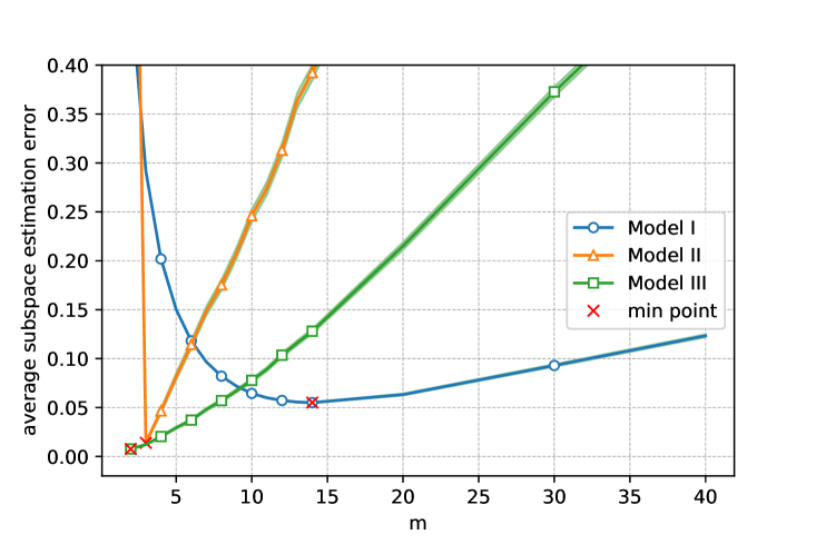
Figure 1: Average subspace estimation error of FSFIR (left), TFSIR (middle) and RFSIR (right) for various models. The standard errors are all below $0.009$.

Figure 1 shows that FSFIR attains the best performance among all models. Moreover, FSFIR is easier to practice as it does not need a slice number $H$ in advance.

5.2 Application to real data

In this section, we analyze the bike sharing data (Fanaee-T and Gama, 2014; Lee and Li, 2022), which includes hourly bike rental counts and weather information such as temperature, precipitation, wind speed, and humidity. The data was collected every day from January 1, 2011 to December 31, 2012 from the Capital Bike Share system in Washington, DC and can be found at https://archive.ics.uci.edu/ml/datasets/Bike+Sharing+Dataset.

The main goal of this section is to investigate how temperature affects bike rentals on Saturdays. After removing data from three Saturdays with significant missing information, we plot hourly bike rental counts and hourly normalized temperature (values divided by 41, the maximum value) for 102 Saturdays in Figure 2. In the following analysis, we use hourly normalized temperature and the logarithm of the daily average bike rental counts as the predictor function and scalar response, respectively.

Figure 2: Bike sharing data

To evaluate the estimation error performance of FSFIR for estimating the central space, we incorporate dimension reduction with FSFIR as an intermediate step in modeling the relationship between the predictor and response variables. Specifically, we apply FSFIR to perform dimension reduction on a given training dataset $\{(\boldsymbol{X}_{i},Y_{i})\}_{i=1}^{n}$. This yields a set of low-dimensional predictors $\boldsymbol{x}_{i}$ for each $i\in[n]$. Subsequently, we utilize Gaussian process regression to fit a nonparametric regression model using the samples $\{(\boldsymbol{x}_{i},Y_{i})\}_{i=1}^{n}$. We randomly selected $90$ samples as the training data and used the remaining data to calculate the out-of-sample mean square error (MSE). We repeated this process $100$ times and calculated the mean and standard error. The results are presented in Table 1, which suggests that FSFIR performs well in practical applications. It is noteworthy that the best result of FSFIR is observed when $d=1$. This means FSFIR provides an accurate and simpler (lower dimensional) model for the relationship between the response variable and the predictor.

	$m$	$1$	$3$	$5$	$7$	$9$	$11$	$13$
FSFIR	$d=1$	0.230	0.259	0.265	0.247	0.280	0.319	0.320
		(0.0097)	(0.0126)	(0.0127)	(0.0122)	(0.0128)	(0.0143)	(0.0160)
	$d=2$		0.356	0.276	0.372	0.334	0.396	0.329
			(0.0409)	(0.0170)	(0.0460)	(0.0312)	(0.0226)	(0.0170)
	$d=3$		0.358	0.461	0.370	0.420	0.625	0.396
			(0.0303)	(0.0507)	(0.0304)	(0.0390)	(0.0795)	(0.0365)
	$d=4$			0.699	0.473	0.726	0.831	0.460
				(0.0544)	(0.0584)	(0.0854)	(0.1008)	(0.0374)
	$d=5$			1.052	0.876	1.131	0.883	0.936
				(0.0710)	(0.0682)	(0.0930)	(0.0942)	(0.0875)

Table 1: The empirical mean (standard error) of MSE.

6 Concluding Remarks

In summary, we introduce two novel objects, the statistics MDDO and the method FSFIR. MDDO serves to measure the conditional mean independence of a functional-valued predictor on a multivariate response. And based on MDDO, FSFIR aims to estimating the central subspace $\mathcal{S}_{\boldsymbol{Y}|\boldsymbol{X}}$.

Besides MDDO, there are other ways to examine the conditional mean independence in functional-data cases, such as the functional martingale difference divergence (FMDD, Lee et al. 2020). However, we would like to point out an extra feature of our MDDO — Under certain circumstances, a low rank projection of $\boldsymbol{X}$ is conditional mean independent of $Y$ even if $\boldsymbol{X}$ is not. In other words, for some $e\in\mathcal{H}$, $\mathbb{E}[\langle e,\boldsymbol{X}\rangle|Y]=\mathbb{E}[\langle e,\boldsymbol{X}\rangle]$ but $\mathbb{E}[\boldsymbol{X}|Y]$ is not equal to $\mathbb{E}[\boldsymbol{X}]$. In this case, we can use MDDO to separate out a part that is conditional mean independent of $Y$ in view of Theorem 1 (ii). This property of MDDO makes it a tool for slicing-free estimation (see the proof of Theorem 2).

However, there are still several open problems that remain to be solved. For example, a study of FSFIR from a decision theoretic point of view is interesting. Additionally, it would be interesting to extend these methods to cases with high-dimensional or functional-valued response. We plan to explore these topics in future research.

Supplementary Materials

Supplement to “Functional Slicing-free Inverse Regression via Martingale Difference Divergence Operator”. The supplementary material includes the proofs for all the theoretical results in the paper.

Songtao Tian, Department of Mathematical Sciences, Tsinghua University E-mail: tst20@mails.tsinghua.edu.cn

Zixiong Yu, Department of Mathematical Sciences, Tsinghua University E-mail: yuzx19@mails.tsinghua.edu.cn

Rui Chen, Center for Statistical Science, Department of Industrial Engineering, Tsinghua University E-mail: chenrui_fzu@163.com

Appendix A Proof of Lemma 1

Proof.

For any ${\boldsymbol{\beta}}\in\mathcal{H}$, according to the definition of $G_{\boldsymbol{s}}$ (see Definition 2), one has

$$\langle G_{\boldsymbol{s}},{\boldsymbol{\beta}}\rangle =\int_{[0,1]}G_{\boldsymbol{s}}(t){\boldsymbol{\beta}}(t)~{}\mathrm{d}t=\int_{[0,1]}\mathrm{cov}\left(\boldsymbol{X}(t),\mathrm{e}^{\mathrm{i}\langle\boldsymbol{s},\boldsymbol{Y}\rangle}\right){\boldsymbol{\beta}}(t)~{}\mathrm{d}t$$

$$=\int_{[0,1]}\mathrm{cov}\left(\boldsymbol{X}(t){\boldsymbol{\beta}}(t),\mathrm{e}^{\mathrm{i}\langle\boldsymbol{s},\boldsymbol{Y}\rangle}\right)~{}\mathrm{d}t.$$

By Fubini theorem, under Assumption 1, one can exchange the order of integration and covariance above and get that

$$\langle G_{\boldsymbol{s}},{\boldsymbol{\beta}}\rangle =\int_{[0,1]}\mathrm{cov}\left(\boldsymbol{X}(t){\boldsymbol{\beta}}(t),\mathrm{e}^{\mathrm{i}\langle\boldsymbol{s},\boldsymbol{Y}\rangle}\right)~{}\mathrm{d}t$$

$$=\mathrm{cov}\left(\int_{[0,1]}\boldsymbol{X}(t){\boldsymbol{\beta}}(t)~{}\mathrm{d}t,\mathrm{e}^{\mathrm{i}\langle\boldsymbol{s},\boldsymbol{Y}\rangle}\right)=\mathrm{cov}\left(\langle\boldsymbol{X},{\boldsymbol{\beta}}\rangle,\mathrm{e}^{\mathrm{i}\langle\boldsymbol{s},\boldsymbol{Y}\rangle}\right).$$

Thus for any $\boldsymbol{\alpha}(t),{\boldsymbol{\beta}}(t)\in\mathcal{H}$, one can get

$$\big{\langle}\big{(}G_{\boldsymbol{s}}\otimes\overline{G}_{\boldsymbol{s}}\big{)}\boldsymbol{\alpha},{\boldsymbol{\beta}}\big{\rangle}=\langle G_{\boldsymbol{s}},\boldsymbol{\alpha}\rangle\langle\overline{G}_{\boldsymbol{s}},{\boldsymbol{\beta}}\rangle=\mathrm{cov}\left(\langle\boldsymbol{X},\boldsymbol{\alpha}\rangle,\mathrm{e}^{\mathrm{i}\langle\boldsymbol{s},\boldsymbol{Y}\rangle}\right)\mathrm{cov}\left(\langle\boldsymbol{X},{\boldsymbol{\beta}}\rangle,\mathrm{e}^{-\mathrm{i}\langle\boldsymbol{s},\boldsymbol{Y}\rangle}\right)$$

$$=\mathbb{E}\left(\langle\boldsymbol{X},\boldsymbol{\alpha}\rangle\mathrm{e}^{\mathrm{i}\langle\boldsymbol{s},\boldsymbol{Y}\rangle}\right)\mathbb{E}\left(\langle\boldsymbol{X},{\boldsymbol{\beta}}\rangle\mathrm{e}^{-\mathrm{i}\langle\boldsymbol{s},\boldsymbol{Y}\rangle}\right)=\mathbb{E}\Big{(}\langle\boldsymbol{X},\boldsymbol{\alpha}\rangle\langle\boldsymbol{X}^{\prime},{\boldsymbol{\beta}}\rangle\mathrm{e}^{\mathrm{i}\langle\boldsymbol{s},\boldsymbol{Y}-\boldsymbol{Y}^{\prime}\rangle}\Big{)}.$$

Considering that $\mathbb{E}\big{(}\langle\boldsymbol{X},\alpha\rangle\langle\boldsymbol{X}^{\prime},{\boldsymbol{\beta}}\rangle\big{)}=0$, one has

$$\big{\langle}\big{(}G_{\boldsymbol{s}}\otimes\overline{G}_{\boldsymbol{s}}\big{)}\boldsymbol{\alpha},{\boldsymbol{\beta}}\big{\rangle}=-\mathbb{E}\Big{(}\langle\boldsymbol{X},\boldsymbol{\alpha}\rangle\langle\boldsymbol{X}^{\prime},{\boldsymbol{\beta}}\rangle\big{(}1-\mathrm{e}^{\mathrm{i}\langle\boldsymbol{s},\boldsymbol{Y}-\boldsymbol{Y}^{\prime}\rangle}\big{)}\Big{)}$$

$$=-\mathbb{E}\Big{(}\langle\boldsymbol{X},\boldsymbol{\alpha}\rangle\langle\boldsymbol{X}^{\prime},{\boldsymbol{\beta}}\rangle\big{[}1-\cos\big{(}\langle\boldsymbol{s},\boldsymbol{Y}-\boldsymbol{Y}^{\prime}\rangle\big{)}\big{]}\Big{)}$$

$$+\mathrm{i}\mathbb{E}\Big{(}\langle\boldsymbol{X},\boldsymbol{\alpha}\rangle\langle\boldsymbol{X}^{\prime},{\boldsymbol{\beta}}\rangle\big{[}\sin\big{(}\langle\boldsymbol{s},\boldsymbol{Y}-\boldsymbol{Y}^{\prime}\rangle\big{)}\big{]}\Big{)}$$ .

It is easy to check that

$$\int_{\mathbb{R}^{q}}\frac{\sin\big{(}\langle\boldsymbol{s},\boldsymbol{Y}-\boldsymbol{Y}^{\prime}\rangle)\big{)}}{\|\boldsymbol{s}\|^{1+q}}~{}\mathrm{d}\boldsymbol{s}=\lim_{\varepsilon\to 0^{+}}\int_{\boldsymbol{s}\in\mathbb{R}^{q}:\varepsilon\leqslant\|\boldsymbol{s}\|\leqslant\varepsilon^{-1}}\frac{\sin\big{(}\langle\boldsymbol{s},\boldsymbol{Y}-\boldsymbol{Y}^{\prime}\rangle\big{)}}{\|\boldsymbol{s}\|^{1+q}}~{}\mathrm{d}\boldsymbol{s}=0,$$

because the integrand is an odd function. By Lemma 1 in Székely et al. (2007), one can also get

$$\int_{\mathbb{R}^{q}}\frac{1-\cos\big{(}\langle\boldsymbol{s},\boldsymbol{Y}-\boldsymbol{Y}^{\prime}\rangle\big{)}}{\|\boldsymbol{s}\|^{1+q}}~{}\mathrm{d}\boldsymbol{s}=c_{q}\|\boldsymbol{Y}-\boldsymbol{Y}^{\prime}\|.$$

Combining above results with Definition 2, one can obtain that

$$\langle\mathrm{MDDO}(\boldsymbol{X}|Y)\boldsymbol{\alpha},{\boldsymbol{\beta}}\rangle=-\mathbb{E}\Big{(}\langle\boldsymbol{X},\boldsymbol{\alpha}\rangle\langle\boldsymbol{X}^{\prime},{\boldsymbol{\beta}}\rangle\|\boldsymbol{Y}-\boldsymbol{Y}^{\prime}\|\Big{)}.$$ (A.1)

Then by the arbitrariness of $\boldsymbol{\alpha},{\boldsymbol{\beta}}\in\mathcal{H}$, the proof is completed. ∎

Appendix B Proof of Theorem 1

According to (A.1), one can get the following useful lemma.

Lemma 4.

Under Assumption 1, for all ${\boldsymbol{\beta}}\in\mathcal{H}$, $\|{\boldsymbol{\beta}}\|=1$, we have

$$\langle\mathrm{MDDO}(\boldsymbol{X}|\boldsymbol{Y})({\boldsymbol{\beta}}),{\boldsymbol{\beta}}\rangle =-\mathbb{E}\Big{[}\langle\boldsymbol{X},{\boldsymbol{\beta}}\rangle\langle\boldsymbol{X}^{\prime},{\boldsymbol{\beta}}\rangle\|\boldsymbol{Y}-\boldsymbol{Y}^{\prime}\|\Big{]}$$

$$=-\mathbb{E}\Big{[}\big{\langle}\langle\boldsymbol{X},{\boldsymbol{\beta}}\rangle{\boldsymbol{\beta}},\langle\boldsymbol{X}^{\prime},{\boldsymbol{\beta}}\rangle{\boldsymbol{\beta}}\big{\rangle}\|\boldsymbol{Y}-\boldsymbol{Y}^{\prime}\|\Big{]}.$$

This conclusion links MDDO with functional martingale difference divergence (FMDD, Lee et al. 2020). Next we give the following two lemmas to finish the proof of Theorem 1.

Lemma 5.

If $T$ is a positive semi-definite operator on a Hilbert space $\widetilde{\mathcal{H}}$, then for all $x\in\widetilde{\mathcal{H}}$, one has $\langle Tx,x\rangle=0\Longleftrightarrow Tx=0$.

Proof.

‘$\Longleftarrow$’: It is obvious.

‘$\Longrightarrow$’: It is easy to check that $f(a,b)=\langle Ta,b\rangle$ $(a,b\in\widetilde{\mathcal{H}})$ is a positive semi-definite Hermitian form. Thus, for any $y\in\widetilde{\mathcal{H}}$, one can use Cauchy inequality to get

$$|\langle Tx,y\rangle|^{2}\leqslant\langle Tx,x\rangle\langle Ty,y\rangle=0\Longrightarrow\langle Tx,y\rangle=0.$$

By the arbitrariness of $y\in\widetilde{\mathcal{H}}$, one has $Tx=0$. ∎

Our proof of Theorem 1 is mainly inspired by the following property of FMDD in Lee et al. (2020).

Lemma 6 (Proposition 1 of Lee et al. (2020)).

If $\mathbb{E}[\|\boldsymbol{X}\|+\|\boldsymbol{Y}\|]<\infty$ and $\mathbb{E}[\|\boldsymbol{X}\|\|\boldsymbol{Y}\|]<\infty$, then we have

$$\mathbb{E}[\langle\boldsymbol{X},\boldsymbol{X}^{\prime}\rangle\|\boldsymbol{Y}-\boldsymbol{Y}^{\prime}\|]=0\Longleftrightarrow\mathbb{E}[\boldsymbol{X}|\boldsymbol{Y}]=0\quad\text{almost surely},$$

where $(\boldsymbol{X}^{\prime},\boldsymbol{Y}^{\prime})$ is an i.i.d. copy of $(\boldsymbol{X},\boldsymbol{Y})$.

Proof of Theorem 1

Proof.

Clearly, (ii) is a direct consequence of Lemma 1 and the following lemma.

Lemma 7 (Lemma 15 in Chen et al. 2023).

If $T$ is an operator defined on $\mathcal{H}_{1}\to\mathcal{H}_{2}$ where $\mathcal{H}_{i},i=1,2$ is a Hilbert space. $\boldsymbol{X}\in\mathcal{H}_{1}$ is a random element satisfying $\mathbb{E}[\boldsymbol{X}]=0$ . Then we have $\mathrm{var}(T\boldsymbol{X})=T\mathrm{var}(\boldsymbol{X})T^{*}$.

Now we start to prove (i). First, one has

$$\mathrm{MDDO}(\boldsymbol{X}|\boldsymbol{Y})=0 \Longleftrightarrow\mathrm{MDDO}(\boldsymbol{X}|\boldsymbol{Y})({\boldsymbol{\beta}})=0,\quad\forall{\boldsymbol{\beta}}\in\mathbb{S}_{\mathcal{H}};$$

$$\mathbb{E}[\boldsymbol{X}|\boldsymbol{Y}]=0~{}~{}\text{a.s.} \Longleftrightarrow\langle\mathbb{E}[\boldsymbol{X}|\boldsymbol{Y}],{\boldsymbol{\beta}}\rangle{\boldsymbol{\beta}}=0~{}~{}\text{a.s.}\quad\forall{\boldsymbol{\beta}}\in\mathbb{S}_{\mathcal{H}},$$

where $\mathbb{S}_{\mathcal{H}}=\{{\boldsymbol{\beta}}\in\mathcal{H}:\|{\boldsymbol{\beta}}\|=1\}$. Second, from Lemma 5, one knows that

$$\mathrm{MDDO}(\boldsymbol{X}|\boldsymbol{Y})({\boldsymbol{\beta}})=0 \Longleftrightarrow\langle\mathrm{MDDO}(\boldsymbol{X}|\boldsymbol{Y})({\boldsymbol{\beta}}),{\boldsymbol{\beta}}\rangle=0.$$

Then under Assumption 1, by Lemma 4 and 6, one has

$$\langle\mathrm{MDDO}(\boldsymbol{X}|\boldsymbol{Y})({\boldsymbol{\beta}}),{\boldsymbol{\beta}}\rangle=0\Longleftrightarrow\mathbb{E}[\big{\langle}\langle\boldsymbol{X},{\boldsymbol{\beta}}\rangle{\boldsymbol{\beta}},\langle\boldsymbol{X}^{\prime},{\boldsymbol{\beta}}\rangle{\boldsymbol{\beta}}\rangle\|\boldsymbol{Y}-\boldsymbol{Y}^{\prime}\|]=0$$

$$\qquad\qquad\qquad\qquad\qquad\Longleftrightarrow\mathbb{E}[\langle\boldsymbol{X},{\boldsymbol{\beta}}\rangle{\boldsymbol{\beta}}|\boldsymbol{Y}]=\langle\mathbb{E}[\boldsymbol{X}|\boldsymbol{Y}],{\boldsymbol{\beta}}\rangle{\boldsymbol{\beta}}=0~{}~{}\text{a.s.}$$

This finishes the proof of Theorem 1. ∎

Appendix C Proof of Lemma 2

Recall the following fact in FSIR.

Lemma 8.

Under Assumption $\ref{as:Linearity condition and Coverage condition}~{}\boldsymbol{\mathrm{{i)}}}$, we have $\mathcal{S}_{\mathbb{E}(\boldsymbol{X}|\boldsymbol{Y})}\subseteq\Gamma\mathcal{S}_{\boldsymbol{Y}|\boldsymbol{X}}\subseteq\mathcal{H}$.

It is a trivial generalization of (Ferré and Yao, 2003, Theorem 2.1) from univariate response to multivariate response.

Proof of Lemma 2

Proof.

First, we prove that $\mathcal{S}_{\mathbb{E}(\boldsymbol{X}|\boldsymbol{Y})}^{\perp}\subseteq\mathrm{Im}\{\mathrm{var(\mathbb{E}(\boldsymbol{X}|\boldsymbol{Y}))}\}^{\perp}$. For any ${\boldsymbol{\beta}}\in\mathcal{S}_{\mathbb{E}(\boldsymbol{X}|\boldsymbol{Y})}^{\perp}$, one has $\langle{\boldsymbol{\beta}},\mathbb{E}(\boldsymbol{X}|\boldsymbol{Y})\rangle=0$ a.s. Then for any $\boldsymbol{\alpha}\in\mathcal{H}$, one can get

$$\langle{\boldsymbol{\beta}},\mathrm{var}(\mathbb{E}(\boldsymbol{X}|\boldsymbol{Y}))\boldsymbol{\alpha}\rangle =\langle{\boldsymbol{\beta}},\mathbb{E}\left[\mathbb{E}(\boldsymbol{X}|\boldsymbol{Y})\otimes\mathbb{E}(\boldsymbol{X}|\boldsymbol{Y})\right]\boldsymbol{\alpha}\rangle$$

$$=\mathbb{E}\big{(}\langle\mathbb{E}(\boldsymbol{X}|\boldsymbol{Y}),\boldsymbol{\alpha}\rangle\langle{\boldsymbol{\beta}},\mathbb{E}(\boldsymbol{X}|\boldsymbol{Y})\rangle\big{)}=0,$$

which means that ${\boldsymbol{\beta}}\in\mathrm{Im}\{\mathrm{var}(\mathbb{E}(\boldsymbol{X}|\boldsymbol{Y}))\}^{\perp}$. Moreover, one has

$$\mathcal{S}_{\mathbb{E}(\boldsymbol{X}|\boldsymbol{Y})}^{\perp}\subseteq\mathrm{Im}\{\mathrm{var}(\mathbb{E}(\boldsymbol{X}|\boldsymbol{Y}))\}^{\perp}\Longrightarrow\overline{\mathcal{S}_{\mathbb{E}(\boldsymbol{X}|\boldsymbol{Y})}}\supseteq\overline{\mathrm{Im}}\{\mathrm{var}(\mathbb{E}(\boldsymbol{X}|\boldsymbol{Y}))\}.$$

Thus, $\overline{\mathrm{Im}}\{\mathrm{var}(\mathbb{E}(\boldsymbol{X}|\boldsymbol{Y}))\}\subseteq\overline{\mathcal{S}_{\mathbb{E}(\boldsymbol{X}|\boldsymbol{Y})}}\subseteq\overline{\Gamma\mathcal{S}_{\boldsymbol{Y}|\boldsymbol{X}}}$ by Lemma 8. According to Assumption 2 ii), one can get

$$\mathrm{dim}\left(\overline{\mathrm{Im}}\{\mathrm{var}(\mathbb{E}(\boldsymbol{X}|\boldsymbol{Y}))\}\right)=\mathrm{dim}\left(\overline{\mathcal{S}_{\mathbb{E}(\boldsymbol{X}|\boldsymbol{Y})}}\right)=\mathrm{dim}(\overline{\Gamma\mathcal{S}_{\boldsymbol{Y}|\boldsymbol{X}}})=d.$$

One can complete the proof since finite dimension subspaces are closed. ∎

Appendix D Proof of Theorem 2

Proof.

For convenience, we abbreviate $\mathrm{MDDO}(\boldsymbol{X}|\boldsymbol{Y})$ to ${M}$. According to Theorem 1 and Lemma 5, one can get

$${\boldsymbol{\beta}}\in\mathcal{S}_{\mathbb{E}(\boldsymbol{X}|\boldsymbol{Y})}^{\perp} \Longleftrightarrow\langle{\boldsymbol{\beta}},\mathbb{E}(\boldsymbol{X}|\boldsymbol{Y})\rangle=0~{}~{}\text{a.s.}\Longleftrightarrow\mathbb{E}(\langle{\boldsymbol{\beta}},\boldsymbol{X}\rangle|\boldsymbol{Y})=0~{}~{}\text{a.s.}$$

$$\Longleftrightarrow\mathrm{MDDO}(\langle{\boldsymbol{\beta}},\boldsymbol{X}\rangle|\boldsymbol{Y})=0\Longleftrightarrow\langle{M}{\boldsymbol{\beta}},{\boldsymbol{\beta}}\rangle=0$$

$$\Longleftrightarrow{M}{\boldsymbol{\beta}}=0\Longleftrightarrow{\boldsymbol{\beta}}\in\mathrm{null}(M)=\overline{\mathrm{Im}}(M)^{\perp},$$

which means that $\mathcal{S}_{\mathbb{E}(\boldsymbol{X}|\boldsymbol{Y})}^{\perp}=\overline{\mathrm{Im}}(M)^{\perp}$ and $\overline{\mathcal{S}_{\mathbb{E}(\boldsymbol{X}|\boldsymbol{Y})}}=\overline{\mathrm{Im}}(M)$. One can complete the proof since finite dimension subspaces are closed. ∎

Appendix E Proof of Lemma 3

Before proving Lemma 3, we give the following lemma.

Lemma 9.

Assume that $P$ is a bounded linear operator from a Hilbert space $\widetilde{\mathcal{H}}$ to itself and $B$ is a positive semi-definite operator from $\widetilde{\mathcal{H}}$ to itself. Then we have $\overline{\mathrm{Im}}(PBP^{*})=\overline{\mathrm{Im}}(PB)$.

Proof.

It suffices to show that $\mathrm{null}(BP^{*})=\mathrm{null}(PBP^{*})$. First, since $B$ is positive semi-definite, one has $\langle x,PBP^{*}x\rangle=\langle P^{*}x,BP^{*}x\rangle\geqslant 0~{}(\forall x\in\widetilde{\mathcal{H}})$. Thus $PBP^{*}$ is a positive semi-definite operator on $\widetilde{\mathcal{H}}$. For any $y\in\widetilde{\mathcal{H}}$, we have

$$PBP^{*}y=0\overset{(a)}{\Longleftrightarrow}\langle y,PBP^{*}y\rangle=\langle P^{*}y,BP^{*}y\rangle=0\overset{(b)}{\Longleftrightarrow}BP^{*}y=0.$$

where $(a)$ and $(b)$ come from Lemma 5. Thus $\mathrm{null}(PBP^{*})=\mathrm{null}(BP^{*})$. ∎

Proof of Lemma 3

Proof.

For convenience, we abbreviate $\mathrm{MDDO}(\boldsymbol{X}|\boldsymbol{Y})$ and $\mathrm{MDDO}(\boldsymbol{X}^{(m)}|\boldsymbol{Y})$ to ${M}$ and $M_{m}$ respectively.

By Corollary 1, one can get $\Gamma\mathcal{S}_{\boldsymbol{Y}|\boldsymbol{X}}=\mathrm{Im}(M)$. Thus,

$$\Pi_{m}\Gamma\mathcal{S}_{\boldsymbol{Y}|\boldsymbol{X}}=\Pi_{m}\mathrm{Im}(M)=\mathrm{Im}(\Pi_{m}M).$$ (E.1)

It is easy to check that

$$\Gamma_{m} :=\mathrm{var}(\boldsymbol{X}^{(m)})=\Pi_{m}\Gamma\Pi_{m}=\Pi_{m}\Gamma=\Gamma\Pi_{m}=\sum\limits_{i=1}^{m}\lambda_{i}\phi_{i}\otimes\phi_{i}.$$ (E.2)

On the one hand, by the definition of $\mathcal{S}^{(m)}_{{\boldsymbol{Y}|\boldsymbol{X}}}$ and $\Gamma_{m}$ (see (4.2) and (E.2)), one can get

$$\Pi_{m}\Gamma\mathcal{S}_{\boldsymbol{Y}|\boldsymbol{X}} =\Pi_{m}\Gamma\Pi_{m}\mathcal{S}_{\boldsymbol{Y}|\boldsymbol{X}}=(\Pi_{m}\Gamma)(\Pi_{m}\mathcal{S}_{\boldsymbol{Y}|\boldsymbol{X}})=\Gamma_{m}\mathcal{S}^{(m)}_{{\boldsymbol{Y}|\boldsymbol{X}}}.$$ (E.3)

On the other hand, one has $\overline{\mathrm{Im}}(\Pi_{m}M)=\overline{\mathrm{Im}}(\Pi_{m}M\Pi_{m})$ by Lemma 9. Since $\Pi_{m}M$ and $\Pi_{m}M\Pi_{m}$ are both of finite rank, one can further get

$$\mathrm{Im}(\Pi_{m}M) =\overline{\mathrm{Im}}(\Pi_{m}M)=\overline{\mathrm{Im}}(\Pi_{m}M\Pi_{m})=\mathrm{Im}(\Pi_{m}M\Pi_{m}).$$

Then according to Theorem 1(ii), one has

$$\mathrm{Im}(\Pi_{m}M)=\mathrm{Im}(\Pi_{m}M\Pi_{m})=\mathrm{Im}(M_{m}).$$ (E.4)

Combining (E.3), (E.4) with (E.1), one has $\Gamma_{m}\mathcal{S}^{(m)}_{{\boldsymbol{Y}|\boldsymbol{X}}}=\mathrm{Im}\{M_{m}\}$. Finally, one can get $\Gamma_{m}^{\dagger}\mathrm{Im}\{M_{m}\}=\Gamma_{m}^{\dagger}\Gamma_{m}\mathcal{S}^{(m)}_{{\boldsymbol{Y}|\boldsymbol{X}}}=\Pi_{m}\mathcal{S}^{(m)}_{{\boldsymbol{Y}|\boldsymbol{X}}}=\mathcal{S}^{(m)}_{{\boldsymbol{Y}|\boldsymbol{X}}}$. ∎

Appendix F Wely Inequality for a Self-adjoint and Compact Operator

First, we show the following three results in standard functional analysis textbook.

Lemma 10 (Spectral theorem).

Let $\widetilde{\mathcal{H}}$ be a Hilbert space and $A:\widetilde{\mathcal{H}}\to\widetilde{\mathcal{H}}$ be a compact, self-adjoint operator. There is an at most countable orthonormal basis $\{\widetilde{e}_{j}\}_{j\in J}$ ($J=\{1,\cdots,n\}$ or $\mathbb{Z}_{\geqslant 1}$) of $\widetilde{\mathcal{H}}$ and eigenvalues $\{\widetilde{\lambda}_{j}\}_{j\in J}$ with $|\widetilde{\lambda}_{1}|\geqslant|\widetilde{\lambda}_{2}|\geqslant\cdots\geqslant 0$ converging to zero, such that

$$x=\sum_{j\in J}\langle x,\widetilde{e}_{j}\rangle\widetilde{e}_{j};\qquad Ax=\sum_{j\in J}\widetilde{\lambda}_{j}\langle x,\widetilde{e}_{j}\rangle\widetilde{e}_{j},\qquad x\in\widetilde{\mathcal{H}}.$$

Lemma 11 (Rayleigh’s principle).

Let $A$ be a compact, self-adjoint operator. If $\{\widetilde{e}_{j}\}_{j\in J}$ and $\{\widetilde{\lambda}_{j}\}_{j\in J}$ are eigenvectors and eigenvalues define in Lemma 10 respectively. Then

$$|\widetilde{\lambda}_{1}|=\mathop{\sup\limits_{\|u\|=1}}|\langle Au,u\rangle|;\qquad|\widetilde{\lambda}_{n}|=\mathop{\sup\limits_{\|u\|=1}}_{u\in\{\widetilde{e}_{1},\cdots,\widetilde{e}_{n-1}\}^{\perp}}|\langle Au,u\rangle|~{}(n\geqslant 2).$$

Lemma 12 (Minimax theorem).

Assume that $A$ is a positive semi-definite and compact operator with its eigenvalues $\{\widetilde{\lambda}_{i}\}$ ordered as $\widetilde{\lambda}_{1}\geqslant\dots\geqslant\widetilde{\lambda}_{n}\geqslant\dots\geqslant 0$, then

$$\widetilde{\lambda}_{n}=\inf_{E_{n-1}}\sup_{x\in E_{n-1}^{\perp},\|x\|=1}\langle Ax,x\rangle$$

where $E_{n-1}$ with dimension $n-1$ is a closed linear subspace of $\widetilde{\mathcal{H}}$.

Then we give the Wely inequality for a self-adjoint and compact operator.

Proposition 4.

Let $M=N+R$ where $M$, $N$ and $R$ are three self-adjoint and compact operators defined on a Hilbert space $\widetilde{\mathcal{H}}$. Also, $M$ and $N$ are positive semi-definite with their respective eigenvalues $\{\mu_{i}\},\{\nu_{i}\}$ ordered as follows

$$M:\mu_{1}\geqslant\dots\geqslant\mu_{n}\geqslant\dots\geqslant 0;\qquad N:\nu_{1}\geqslant\dots\geqslant\nu_{n}\geqslant\dots\geqslant 0,$$

while $R$’s eigenvalues are $\{\rho_{i}\}$ ordered as follows:

$$R:|\rho_{1}|\geqslant\dots\geqslant|\rho_{n}|\geqslant\dots\geqslant 0.$$

Then the following inequalities hold: $|\mu_{k}-\nu_{k}|\leqslant|\rho_{1}|=\|R\|$, $k\geqslant 1$.

Proof.

From Lemma 12, we have:

$$\mu_{n}=\inf_{E_{n-1}}\sup_{x\in E_{n-1}^{\perp},\|x\|=1}\langle Mx,x\rangle;\qquad\nu_{n}=\inf_{E_{n-1}}\sup_{x\in E_{n-1}^{\perp},\|x\|=1}\langle Nx,x\rangle,$$

where $E_{n-1}$ with dimension $n-1$ is a closed linear subspace of $\widetilde{\mathcal{H}}$. By Lemma 11, we have:

$$\sup_{\|u\|=1}|\langle Ru,u\rangle|=|\rho_{1}|.$$

Since $\langle Mu,u\rangle=\langle Nu,u\rangle+\langle Ru,u\rangle$, for any $\|u\|=1$, we have:

$$\langle Nu,u\rangle-|\rho_{1}|\leqslant\langle Mu,u\rangle\leqslant\langle Nu,u\rangle+|\rho_{1}|.$$

Then for any given $n-1$ dimensional closed linear subspace of $\widetilde{\mathcal{H}}$, we conclude

$$\sup_{u\in E_{n-1}^{\perp},\|u\|=1}\langle Nu,u\rangle-|\rho_{1}|\leqslant\sup_{u\in E_{n-1}^{\perp},\|u\|=1}\langle Mu,u\rangle\leqslant\sup_{u\in E_{n-1}^{\perp},\|u\|=1}\langle Nu,u\rangle+|\rho_{1}|.$$ (F.1)

Take the infimum with respective to $E_{n-1}$ in (F.1), we have

$$\nu_{n}-|\rho_{1}|\leqslant\mu_{n}\leqslant\nu_{n}+|\rho_{1}|$$

by Lemma 12. ∎

The next result is a direct corollary of Proposition 4.

Corollary 2.

Let $M$ and $N$ be two self-adjoint, positive semi-definite and compact operators defined on a Hilbert space $\widetilde{\mathcal{H}}$ with their respective eigenvalues $\{\mu_{i}\},\{\nu_{i}\}$ ordered as follows

$$M:\mu_{1}\geqslant\dots\geqslant\mu_{n}\geqslant\dots\geqslant 0\quad\text{and}\quad N:\nu_{1}\geqslant\dots\geqslant\nu_{n}\geqslant\dots\geqslant 0.$$

Then the following inequalities hold: $|\mu_{k}-\nu_{k}|\leqslant\|M-N\|$, $k\geqslant 1$.

Appendix G Proof of Proposition 2

Before proving Proposition 2, we give the following conclusion, whose proof is deferred to the end of this section.

Proposition 5.

Under Assumptions 1 and 3, for all $\gamma\in(0,1/2)$, there exist positive constants $D_{0}=D_{0}(\gamma,\sigma_{0},\sigma_{1})$, $D_{1}=D_{1}(\sigma_{1})$, $D_{2}=D_{2}(\sigma_{0},\sigma_{1})$ and $n_{0}=n_{0}(\gamma,\sigma_{0},\sigma_{1})$ such that for all $n\geqslant n_{0}$ and

$$C\in\left(D_{0}n^{\frac{2\gamma}{5}}-\ln\left(D_{1}m^{2}n\right),D_{2}n^{\frac{1}{5}}-\ln\left(D_{1}m^{2}n\right)\right],$$

we have

$$\mathbb{P}\left(\left\|\widehat{M}_{m}-M_{m}\right\|<\left(\frac{C+\ln(D_{1}m^{2}n)}{D_{2}}\right)^{\frac{5}{2}}\frac{12m}{\sqrt{n}}\right)\geqslant 1-\exp(-C).$$

Proof of Proposition 2

Proof.

Using Corollary 2, one can get $\lambda_{i}\left(\widehat{M}_{m}\right)\leqslant\left\|\widehat{M}_{m}-M_{m}\right\|+\lambda_{i}\left(M_{m}\right)$. Since $\mathrm{rank}(M_{m})=d$, one can get $\lambda_{i}(M_{m})=0,~{}i\geqslant d+1$. Thus by Proposition 5, one has

$$\mathbb{P}\left(\lambda_{d+1}(\widehat{M}_{m})<\left(\frac{C+\ln\left(D_{1}m^{2}n\right)}{D_{2}}\right)^{\frac{5}{2}}\frac{12m}{\sqrt{n}}\right)\geqslant 1-\exp(-C)\qquad(i\geq d+1).$$ (G.1)

Notice that

$$\left\|\widehat{M}_{m}^{d}-M_{m}\right\| \leqslant\left\|M_{m}-\widehat{M}_{m}\right\|+\left\|\widehat{M}_{m}-\widehat{M}_{m}^{d}\right\|;$$

$$\left\|\widehat{M}_{m}-\widehat{M}_{m}^{d}\right\| =\left\|\sum_{i=d+1}^{\infty}\widehat{\mu}_{i}\widehat{\gamma}_{i}\otimes\widehat{\gamma}_{i}\right\|=\widehat{\lambda}_{d+1}=\lambda_{d+1}(\widehat{M}_{m})$$

by (4.4). Then combing Proposition 5 with (G.1) can complete the proof. ∎

Proof of Proposition 5

Proof.

Note that $\boldsymbol{X}^{(m)}=\sum\limits_{j=1}^{m}\langle\boldsymbol{X},\phi_{j}\rangle\phi_{j}$, then a simple calculation leads to

$$M_{m} =-\sum_{i,j=1}^{m}\mathbb{E}\big{[}\langle\boldsymbol{X},\phi_{i}\rangle\langle\boldsymbol{X}^{\prime},\phi_{j}\rangle\|\boldsymbol{Y}-\boldsymbol{Y}^{\prime}\|\big{]}\phi_{i}\otimes\phi_{j};$$

$$\widehat{M}_{m} =-\sum_{i,j=1}^{m}\frac{1}{n^{2}}\sum_{k,\ell=1}^{n}\langle\boldsymbol{X}_{k},\phi_{i}\rangle\langle\boldsymbol{X}_{\ell},\phi_{j}\rangle\|\boldsymbol{Y}_{k}-\boldsymbol{Y}_{\ell}\|\phi_{i}\otimes\phi_{j}.$$

For a operator $\Gamma^{\prime}$ that can be expanded as $\Gamma^{\prime}:=\sum\limits_{i,j=1}^{\infty}a_{ij}\phi_{i}\otimes\phi_{j}$, let us define its maximal norm as $\|\Gamma^{\prime}\|_{\mathrm{max}}=\sup\limits_{i,j}|a_{ij}|$.

Lemma 13.

(Mai et al., 2023, Theorem 1) Under Assumptions 1 and 3, for all $\gamma\in(0,1/2)$, there exist positive constants $C_{0}=C_{0}(\gamma,\sigma_{0},\sigma_{1})$, $C_{1}=C_{1}(\sigma_{1})$, $C_{2}=C_{2}(\sigma_{0};\sigma_{1})$ and $n_{0}=n_{0}(\gamma,\sigma_{0},\sigma_{1})$ such that for all $n\geqslant n_{0}$ and $\varepsilon\in(C_{0}n^{-(1/2-\gamma)},1]$, we have

$$\mathbb{P}\left(\left\|\widehat{M}_{m}-M_{m}\right\|_{\max}>12\varepsilon\right)\leqslant C_{1}m^{2}n\exp\left(-C_{2}\left(\varepsilon^{2}n\right)^{1/5}\right).$$

Since $\left\|\widehat{M}_{m}-M_{m}\right\|\leqslant m\left\|\widehat{M}_{m}-M_{m}\right\|_{\mathrm{max}}$, one has

$$\mathbb{P}\left(\left\|\widehat{M}_{m}-M_{m}\right\|>12m\varepsilon\right)\leqslant C_{1}m^{2}n\exp\left(-C_{2}\left(\varepsilon^{2}n\right)^{1/5}\right).$$

Let $C=C_{2}\left(\varepsilon^{2}n\right)^{1/5}-\ln\left(C_{1}m^{2}n\right)$ satisfying

$$C\in\left(C_{2}C_{0}^{2/5}n^{2\gamma/5}-\ln\left(C_{1}m^{2}n\right),C_{2}n^{1/5}-\ln\left(C_{1}m^{2}n\right)\right],$$

then one has

$$\mathbb{P}\left(\left\|\widehat{M}_{m}-M_{m}\right\|\leqslant\left(\frac{C+\ln\left(C_{1}m^{2}n\right)}{C_{2}}\right)^{\frac{5}{2}}\frac{12m}{\sqrt{n}}\right)>1-\exp(-C).$$

Then in order to complete the proof, one only need to choose $D_{0}$, $D_{1}$ and $D_{2}$ to be $C_{2}C_{0}^{2/5}$, $C_{1}$ and $C_{2}$ respectively. ∎

Appendix H Properties of Sub-Gaussian Random Vectors

We first review the definition of sub-Gaussian random variables.

Definition 3 (Sub-Gaussian random variable and its upper-exponentially bounded constant).

A random variable $X$ is called a sub-Gaussian random variable if $X$ satisfies one of the following equivalent properties:

• Tails. $\mathbb{P}(|X|>t)\leqslant\exp(1-t^{2}/K^{2}_{1})$ for any $t>0$;

• Moments. $\mathbb{E}[|X|^{p}]^{1/p}\leqslant K_{2}\sqrt{p}$ for any $p\geqslant 1$;

• Super-exponential moment: $\mathbb{E}[\exp(X^{2}/K^{2}_{3})]\leqslant\mathrm{e}$.

  Moreover, if $\mathbb{E}[X]=0$, then the properties $1)-3)$ are also equivalent to the following one:

• Moment generating function: $\mathbb{E}[\exp(tX)]\leqslant\exp(t^{2}K^{2}_{4})$ for all $t\in\mathbb{R}$.

Here $K_{1}$, $K_{2}$, $K_{3}$ and $K_{4}$ are four constants. $K$ is called an upper-exponentially bounded constant of $X$ if $K\geqslant\max\{K_{1},K_{2},K_{3},K_{4}\}$.

Definition 4 (Sub-Gaussian random vector and its upper-exponentially bounded constant).

${X}\in\mathbb{R}^{m}$ is called a sub-Gaussian random vector if for all $x\in\mathbb{R}^{m}$, one-dimensional marginal $\langle{X},x\rangle$ is sub-Gaussian random variable. $K$ is called an upper-exponentially bounded constant of $X$ if $K$ satisfies:

$$K\geqslant\sup_{x\in\mathbb{S}^{m-1}}K(\langle X,x\rangle)$$

where $K(\langle X,x\rangle)$ denotes an upper-exponentially bounded constant of $\langle X,x\rangle$. Moreover, $K$ is called a uniform (about $m$) upper-exponentially bounded constant of $X$ if $K$ satisfies:

$$K\geqslant\sup_{m}\sup_{x\in\mathbb{S}^{m-1}}K\left(\langle X,x\rangle\right).$$

Furthermore, $X$ is called a uniform (about $m$) sun-Gaussian random vector.

The following is an application of sub-Gaussian random vectors.

Lemma 14 (Vershynin 2010).

Let $\boldsymbol{M}=[\boldsymbol{m}_{1}~{}\cdots~{}\boldsymbol{m}_{n}]$ be an $m\times n$ matrix ($n>m$) whose columns $\boldsymbol{m}_{i}$ are independent centered sub-Gaussian random vectors with covariance matrix $\mathbf{I}_{m}$. Let $\sigma^{+}_{\min}(\boldsymbol{M})$ and $\sigma_{\max}(\boldsymbol{M})$ be the infimum and supremum of positive singular values of $\boldsymbol{M}$ respectively. Then, for any $t>0$, with probability at least $1-2\exp(-C^{\prime}t^{2})$, we have

$$\sqrt{n}-C_{0}\sqrt{m}-t\leqslant\sigma^{+}_{\min}(\boldsymbol{M})\leqslant\sigma_{\max}(\boldsymbol{M})\leqslant\sqrt{n}+C_{0}\sqrt{m}+t$$

where $C^{\prime}$ and $C_{0}$ are two positive constants depending only on $K(\boldsymbol{m}_{1})$: the upper-exponentially bounded constant of $\boldsymbol{m}_{1}$.

Let $t=\sqrt{m}$, then one can easily get

$$\begin{split}\lambda_{\max}\left(\frac{1}{n}\boldsymbol{M}\boldsymbol{M}^{\top}\right)\leqslant\left(1+\frac{(C_{0}+1)\sqrt{m}}{\sqrt{n}}\right)^{2};\\ \lambda_{\min}^{+}\left(\frac{1}{n}\boldsymbol{M}\boldsymbol{M}^{\top}\right)\geqslant\left(1-\frac{(C_{0}+1)\sqrt{m}}{\sqrt{n}}\right)^{2},\end{split}$$ (H.1)

with probability at least $1-2\exp(-C^{\prime}m)$ where $\lambda^{+}_{\min}(\cdot)$ and $\lambda_{\max}(\cdot)$ stands for the infimum and supremum of the positive spectrum respectively.

Lemma 15.

Assume that $\boldsymbol{x}_{1},\boldsymbol{x}_{2},...,\boldsymbol{x}_{n}$ are $n$ i.i.d. samples from an $m$-dimensional centered sub-Gaussian vector with an invertible covariance matrix $\Sigma$. Let $\widehat{\Sigma}:=\frac{1}{n}\sum_{i}\boldsymbol{x}_{i}\boldsymbol{x}_{i}^{\top}$. Then there exists a positive constant $n_{1}^{\prime}=n_{1}^{\prime}(K(\boldsymbol{m}_{1}),c_{1})$ ($c_{1}$ is defined in (4.1)), such that when $n\geqslant n_{1}^{\prime}$, we have

$$\left\|\widehat{\Sigma}-\Sigma\right\| \leqslant(C_{0}+2)^{2}\lambda_{\max}(\Sigma)\sqrt{\frac{m}{n}}~{}~{}\text{and}~{}~{}\left\|\widehat{\Sigma}^{-1}-\Sigma^{-1}\right\|\leqslant\frac{4(C_{0}+2)^{2}}{\lambda_{\min}(\Sigma)}\sqrt{\frac{m}{n}},$$

with probability at least $1-2\exp(-C^{\prime}m)$, where $C_{0}$ is defined in Lemma 14.

Proof.

Let $\boldsymbol{x}_{i}=\Sigma^{\frac{1}{2}}\boldsymbol{m}_{i}$ and $\boldsymbol{M}=[\boldsymbol{m}_{1}~{}\cdots~{}\boldsymbol{m}_{n}]$ where $\boldsymbol{m}_{i}$ is a centered sub-Gaussian random vector with covariance $\mathbf{I}_{m}$. Then one has

$$\left\|\widehat{\Sigma}-\Sigma\right\| \leqslant\left\|\Sigma^{\frac{1}{2}}\right\|\cdot\left\|\frac{1}{n}\boldsymbol{M}\boldsymbol{M}^{\top}-\mathbf{I}\right\|\cdot\left\|\Sigma^{\frac{1}{2}}\right\|$$

$$=\lambda_{\max}(\Sigma)\cdot\left[\lambda_{\max}\left(\frac{1}{n}\boldsymbol{M}\boldsymbol{M}^{\top}\right)-1\right]$$

and

$$\left\|\widehat{\Sigma}^{-1}-\Sigma^{-1}\right\| \leqslant\left\|\Sigma^{-\frac{1}{2}}\right\|\cdot\left\|\frac{1}{n}\boldsymbol{M}\boldsymbol{M}^{\top}-\mathbf{I}\right\|\cdot\left\|\left(\frac{1}{n}\boldsymbol{M}\boldsymbol{M}^{\top}\right)^{-1}\right\|\cdot\left\|\Sigma^{-\frac{1}{2}}\right\|$$

$$=\frac{1}{\lambda_{\min}(\Sigma)}\left[\lambda_{\max}\left(\frac{1}{n}\boldsymbol{M}\boldsymbol{M}^{\top}\right)-1\right]\cdot\lambda_{\min}\left(\frac{1}{n}\boldsymbol{M}\boldsymbol{M}^{\top}\right)^{-1}.$$

By (H.1), it is easy to check that

$$\lambda_{\max}\left(\frac{1}{n}\boldsymbol{M}\boldsymbol{M}^{\top}\right)-1\leqslant\left(1+\frac{(C_{0}+1)\sqrt{m}}{\sqrt{n}}\right)^{2}-1\leqslant\frac{(C_{0}+2)^{2}\sqrt{m}}{\sqrt{n}};$$

$$\lambda_{\min}\left(\frac{1}{n}\boldsymbol{M}\boldsymbol{M}^{\top}\right)\geqslant\left(1-\frac{(C_{0}+1)\sqrt{m}}{\sqrt{n}}\right)^{2}\geqslant\frac{1}{4}~{}\text{for}~{}n\geqslant[2(C_{0}+1)]^{\frac{2}{1-c_{1}}},$$

with probability at least $1-2\exp(-C^{\prime}m)$. Thus the proof is completed by choosing $n_{1}^{\prime}(C_{0},c_{1}):=[2(C_{0}+1)]^{\frac{2}{1-c_{1}}}$. ∎

Appendix I Proof of Proposition 3

We first give the following lemma whose proof is deferred to the end of this section.

Lemma 16.

If $T$ is of finite rank, then we have $\lim\limits_{m\to\infty}\|\Pi_{m}T\Pi_{m}-T\|=0$.

A direct corollary of this lemma is as follows.

Corollary 3.

Under Assumptions 1 and 2, we have $\lim\limits_{m\to\infty}\|M-M_{m}\|=0$.

We denote by $m_{M}(\varepsilon)$ the minimal integer $m_{M}$ satisfying $\|M-M_{m}\|\leqslant\varepsilon$ for all $m\geqslant m_{M}$.

Proposition 3 is a direct corollary of the following Proposition.

Proposition 6.

Suppose that Assumptions 1 to 4 hold, then $\forall\gamma\in(0,1/2)$, there exist positive constants

$$n_{1}=n_{1}(\gamma,\sigma_{0},\sigma_{1},\boldsymbol{K},m_{M}(1),c_{1}),\quad D_{3}=D_{3}(\|M\|,\widetilde{C},\boldsymbol{K})$$

and $C^{\prime}=C^{\prime}(\boldsymbol{K})$ , such that when $n\geqslant n_{1}$, we have

$$\mathbb{P}\left(\left\|\widehat{\Gamma}_{m}^{\dagger}\widehat{M}_{m}^{d}-\Gamma_{m}^{\dagger}M_{m}\right\|\leqslant\left[\frac{C+\ln(D_{1}m^{2}n)}{D_{2}}\right]^{\frac{5}{2}}\frac{24m^{\alpha_{1}+1}}{\widetilde{C}\sqrt{n}}+D_{3}\frac{m^{(2\alpha_{1}+1)/2}}{n^{1/2}}\right)$$

$$\geqslant 1-\exp(-C)-2\exp(-C^{\prime}m).$$

Here $D_{1},D_{2}$ and $C$ are defined in Proposition 2 and $\boldsymbol{K}$ is the uniform upper-exponentially bounded constant of $(\sqrt{\lambda_{1}}w_{1},\dots,\sqrt{\lambda_{m}}w_{m})$.

Proof.

By triangle inequality, one has

$$\left\|\widehat{\Gamma}_{m}^{\dagger}\widehat{M}_{m}^{d}-\Gamma_{m}^{\dagger}M_{m}\right\|=\left\|\widehat{\Gamma}_{m}^{\dagger}\widehat{M}_{m}^{d}-\widehat{\Gamma}_{m}^{\dagger}M_{m}+\widehat{\Gamma}_{m}^{\dagger}M_{m}-\Gamma_{m}^{\dagger}M_{m}\right\|$$

$$\qquad\leqslant\left\|\Gamma_{m}^{\dagger}\right\|\cdot\left\|\widehat{M}_{m}^{d}-M_{m}\right\|+\left\|\widehat{\Gamma}_{m}^{\dagger}-\Gamma_{m}^{\dagger}\right\|\cdot\left\|M_{m}\right\|.$$

Thus one can bound $\left\|\Gamma_{m}^{{\dagger}}M_{m}-\widehat{\Gamma}_{m}^{{\dagger}}\widehat{M}_{m}^{d}\right\|$ by bound $\left\|\Gamma_{m}^{\dagger}\right\|$, $\left\|\widehat{\Gamma}_{m}^{\dagger}-\Gamma_{m}^{\dagger}\right\|$, $\left\|\widehat{M}_{m}^{d}-M_{m}\right\|$ and $\left\|M_{m}\right\|$ respectively.

• Bound of $\left\|\Gamma_{m}^{\dagger}\right\|$: By Assumption 4, one has

  $$\lambda_{j}\geqslant\widetilde{C}j^{-\alpha_{1}}\Rightarrow\left\|\Gamma_{m}^{\dagger}\right\|=\lambda_{m}^{-1}\leqslant\widetilde{C}^{-1}m^{\alpha_{1}}.$$ (I.1)

• Bound of $\left\|\widehat{\Gamma}_{m}^{\dagger}-\Gamma_{m}^{\dagger}\right\|$: Let us define $\mathcal{H}_{m}:=\mathrm{span}\{\phi_{1},\dots,\phi_{m}\}$ where $\{\phi_{i}\}$ is introduced in Equation $\eqref{eq:X expansion}$. It is easy to check that $\left\|\widehat{\Gamma}_{m}^{\dagger}-\Gamma_{m}^{\dagger}\right\|=\left\|(\widehat{\Gamma}_{m}^{\dagger}-\Gamma_{m}^{\dagger})|_{\mathcal{H}_{m}}\right\|$ since $\left(\widehat{\Gamma}_{m}^{\dagger}-\Gamma_{m}^{\dagger}\right){\boldsymbol{\beta}}=0$ for any ${\boldsymbol{\beta}}\in\mathcal{H}_{m}^{\perp}$. Because $\left(\widehat{\Gamma}_{m}^{\dagger}-\Gamma_{m}^{\dagger}\right)|_{\mathcal{H}_{m}}$ can be represented by matrix $\widehat{\Sigma}^{-1}-\Sigma^{-1}$ defined in Lemma 15 under orthonormal basis $\{\phi_{i}\}_{i=1}^{m}$, one can get $\left\|\widehat{\Gamma}_{m}^{\dagger}-\Gamma_{m}^{\dagger}\right\|=\|\widehat{\Sigma}^{-1}-\Sigma^{-1}\|$. Similarly, one can also get $\left\|\Gamma_{m}^{\dagger}\right\|=\left\|\Sigma^{-1}\right\|=\lambda_{\min}^{-1}(\Sigma)$. Thus, by Lemma 15 one has

  $$\mathbb{P}\left(\left\|\widehat{\Gamma}_{m}^{\dagger}-\Gamma_{m}^{\dagger}\right\|\leqslant{4(C_{0}+2)^{2}}\left\|\Gamma^{{\dagger}}_{m}\right\|\sqrt{\frac{m}{n}}\right)\geqslant 1-2\exp(-C^{\prime}m)$$

  for sufficiently large $n\geqslant n_{1}^{\prime}(\boldsymbol{K},c_{1})$ . Combing with $\left\|\Gamma_{m}^{\dagger}\right\|\leqslant\widetilde{C}^{-1}m^{\alpha_{1}}$, one can get

  $$\mathbb{P}\left(\left\|\widehat{\Gamma}_{m}^{\dagger}-\Gamma_{m}^{\dagger}\right\|\leqslant\frac{4(C_{0}+2)^{2}m^{(2\alpha_{1}+1)/2}}{\widetilde{C}n^{1/2}}\right)\geqslant 1-2\exp(-C^{\prime}m)$$ (I.2)

  for sufficiently large $n\geqslant n_{1}^{\prime}(\boldsymbol{K},c_{1})$.

• Bound of $\left\|\widehat{M}_{m}^{d}-M_{m}\right\|$: See Proposition 2.

• Bound of $\left\|M_{m}\right\|$: By Corollary 3, $\|M-M_{m}\|\leqslant 1$ for sufficiently large $m\geqslant m_{M}(1)$. Then by triangle inequality, one can get

  $$\|M_{m}\|-\|M\|\leqslant\|M-M_{m}\|\leqslant 1.$$

  Hence,

  $$\|M_{m}\|\leqslant\|M\|+1.$$ (I.3)

Combing (I.1), (I.2), Proposition 2 with (I.3), one can choose $D_{3}$ and $n_{1}$ to be $\frac{4(C_{0}+2)^{2}(\|M\|+1)}{\widetilde{C}}$ and $\max\{n_{0},n_{1}^{\prime}(\boldsymbol{K},c_{1}),m_{M}(1)^{1/c_{1}}\}$ respectively to complete the proof where $n_{0}$ is defined in Proposition 2. ∎

Proof of Lemma 16

Proof.

By the triangle inequality and compatibility of operator norm, one has

$$\|\Pi_{m}T\Pi_{m}-T\| \leqslant\|\Pi_{m}T\Pi_{m}-\Pi_{m}T\|+\|\Pi_{m}T-T\|$$

$$\leqslant\|(\Pi_{m}-I)T^{*}\|+\|(\Pi_{m}-I)T\|$$

where $I=\sum\limits_{i=1}^{\infty}\phi_{i}\otimes\phi_{i}$ for $\{\phi_{i}\}_{i\in\mathbb{Z}_{\geqslant 1}}$ defined in (2.1) being an orthonormal basis of $\mathcal{H}$.

Since $T$ is of finite rank, let us assume that $\{e_{i}\}_{i=1}^{k}$ is an orthonormal basis of $\mathrm{Im}(T)$ where $k=\mathrm{rank}(T)$. For any ${\boldsymbol{\beta}}\in\mathcal{H}$ such that $\|{\boldsymbol{\beta}}\|=1$, one has $\|T{\boldsymbol{\beta}}\|\leqslant\|T\|\|{\boldsymbol{\beta}}\|=\|T\|$, so one can assume that $T{\boldsymbol{\beta}}\in\mathrm{Im}(T)$ admits the following expansion under basis $\{e_{i}\}_{i=1}^{k}$:

$$T{\boldsymbol{\beta}}=\sum_{i=1}^{k}b_{i}e_{i},\quad\sum_{i=1}^{k}b^{2}_{i}\leqslant\|T\|^{2}<\infty.$$

Thus

$$\|(I-\Pi_{m})T{\boldsymbol{\beta}}\|=\left\|\sum_{i=1}^{k}(I-\Pi_{m})b_{i}e_{i}\right\|\leqslant\sum_{i=1}^{k}|b_{i}|\cdot\|(I-\Pi_{m})e_{i}\|.$$

Clearly, $\|(\Pi_{m}-I)\alpha\|~{}(\forall\alpha\in\mathcal{H})$ tends to $0$ as $m\to\infty$ since

$$(I-\Pi_{m})\alpha=\left(\sum_{i={m+1}}^{\infty}\phi_{i}\otimes\phi_{i}\right)\left(\sum\limits_{i=1}^{\infty}c_{i}\phi_{i}\right)=\sum_{i=m+1}^{\infty}c_{i}\phi_{i}\xrightarrow{m\to\infty}0$$

where we have assumed that $\alpha=\sum\limits_{i=1}^{\infty}c_{i}\phi_{i}$ .

Thus $\forall\varepsilon>0$, there exists some $N_{i}>0$ such that $\forall m>N_{i}$ one has $\|(\Pi_{m}-I)e_{i}\|<\varepsilon$, $(\forall i=1,...,k)$. Let $N=\max\{N_{1},\cdots,N_{k}\}$, then $\forall m>N$ one has

$$\|(I-\Pi_{m})T{\boldsymbol{\beta}}\|\leqslant\sum_{i=1}^{k}|b_{i}|\cdot\|(I-\Pi_{m})e_{i}\|\leqslant\sum_{i=1}^{k}|b_{i}|\varepsilon\leqslant k\varepsilon\|T\|,$$

which means that $\forall m>N$, one has

$$\|(\Pi_{m}-I)T\| =\sup_{\|{\boldsymbol{\beta}}\|=1}\|(\Pi_{m}-I)T{\boldsymbol{\beta}}\|\leqslant k\varepsilon\|T\|.$$

Thus $\lim\limits_{m\to\infty}\|(\Pi_{m}-I)T\|=0$.

Similarly, one can also get $\lim\limits_{m\to\infty}\|(\Pi_{m}-I)T^{*}\|=0$. Then the proof of Lemma 16 is completed. ∎

Appendix J Sin Theta Theorem

J.1 Sin Theta Theorem for Self-adjoint Operators

Lemma 17 (Proposition 2.3 in Seelmann (2014)).

Let $B$ be a self-adjoint operator on a separable Hilbert space $\widetilde{\mathcal{H}}$, and let ${V}\in\mathcal{L}(\widetilde{\mathcal{H}})$ be another self-adjoint operator where $\mathcal{L}\left(\widetilde{\mathcal{H}}\right)$ stands for the space of bounded linear operators from a Hilbert space $\widetilde{\mathcal{H}}$ to $\widetilde{\mathcal{H}}$. Write the spectra of $B$ and $B+V$ as

$$\mathrm{spec}(B)=\sigma\cup\Sigma\quad\text{and}\quad\mathrm{spec}(B+V)=\omega\cup\Omega$$

with $\sigma\cap\Sigma=\varnothing=\omega\cap\Omega$, and suppose that there is $\widehat{d}>0$ such that

$$\mathrm{dist}(\sigma,\Omega)\geqslant\widehat{d}\quad\text{and}\quad\mathrm{dist}(\Sigma,\omega)\geqslant\widehat{d}$$

where $\mathrm{d}ist(\sigma,\Sigma):=\min\{|a-b|:a\in\sigma,b\in\Omega\}$. Then it holds that

$$\|P_{{B}}(\sigma)-P_{{B}+{V}}(\omega)\|\leqslant\frac{\pi}{2}\frac{\|V\|}{\widehat{d}}$$

where $P_{B}(\sigma)$ denotes the spectral projection for $B$ associated with $\sigma$, i.e.,

$$P_{B}(\sigma):=\frac{1}{2\pi\mathrm{i}}\oint_{\gamma}\frac{\mathrm{d}z}{z-B},$$

where $\gamma$ is a contour on $\mathbb{C}$ that encloses $\sigma$ but no other elements of $\mathrm{spec}(B)$.

Remark 5.

We note that, if further $B$ is compact, the spectral projection coincide with projection operator onto the closure of the space spanned by the eigenfunctions associated with the eigenvalues in $\sigma$.

Specifically, if $B$ is compact, by the spectral decomposition theorem one has

$$B=\sum_{i=1}^{\infty}\mu_{i}e_{i}\otimes e_{i}\quad\text{and}\quad(z-B)^{-1}=\sum_{i=1}^{\infty}(z-\mu_{i})^{-1}e_{i}\otimes e_{i},$$

where $\mathrm{spec}(B):=\{\mu_{i}\}_{i=1}^{\infty}$ satisfies $|\mu_{i}|\xrightarrow{i\to\infty}0$. Then $\forall v\in\mathcal{H}$, it holds that

$$P_{B}(\sigma)v =\frac{1}{2\pi\mathrm{i}}\oint_{\gamma}({z-B})^{-1}v~{}{\mathrm{d}z}=\frac{1}{2\pi\mathrm{i}}\oint_{\gamma}\sum_{i=1}^{\infty}(z-\mu_{i})^{-1}\langle e_{i},v\rangle e_{i}~{}{\mathrm{d}z}$$

$$=\sum_{i=1}^{\infty}\left[\left(\frac{1}{2\pi\mathrm{i}}\oint_{\gamma}(z-\mu_{i})^{-1}~{}{\mathrm{d}z}\right)\langle e_{i},v\rangle e_{i}\right]=\sum_{i\in\{i:\mu_{i}\in\sigma\}}\langle e_{i},v\rangle e_{i}.$$

In particular, if $\sigma=\mathrm{spec}(B)\backslash\{0\}$, then $P_{B}(\sigma)$ is the projection operator onto the $\overline{\mathrm{Im}}(B)$.

Splitting eigenvalues into nonzero part and zero part yields the following useful corollary.

Corollary 4.

Let $B$ and $B^{\prime}$ be two positive semi-definite and compact operators with finite rank on a separable Hilbert space $\widetilde{\mathcal{H}}$. Let $\lambda_{\min}^{+}(B)$ and $\lambda_{\min}^{+}(B^{\prime})$ be the infimum of the positive eigenvalues of ${B}$ and ${B}^{\prime}$ respectively. Then we have

$$\left\|P_{B}-P_{B^{\prime}}\right\|\leqslant\frac{\pi}{2}\frac{\|B-B^{\prime}\|}{\min\{\lambda_{\min}^{+}(B),\lambda_{\min}^{+}(B^{\prime})\}}.$$

J.2 Sin Theta Theorem for General Operators

When ${B}$ and ${V}$ in Lemma 17 are not self-adjoint, we use the symmetrization trick, which mainly depends on the following Lemma.

Lemma 18.

$P_{A}=P_{AA^{*}}$ for any bounded linear operator $A$ from a Hilbert space $\widetilde{\mathcal{H}}$ to $\widetilde{\mathcal{H}}$. Especially, $P_{A}=P_{AA^{\top}}$ for any matrix $A$.

Proof.

First we show that the null space of $A^{*}$ is the same as the null space of $AA^{*}$. On the one hand,

$$x\in\mathrm{null}(A^{*})\Longrightarrow A^{*}x=0\Longrightarrow AA^{*}x=0\Longrightarrow x\in\mathrm{null}(AA^{*});$$

One the other hand,

$$x\in\mathrm{null}(AA^{*}) \Longrightarrow AA^{*}x=0\Longrightarrow\langle x,AA^{*}x\rangle=\langle A^{*}x,A^{*}x\rangle=\|A^{*}x\|^{2}=0$$

$$\Longrightarrow A^{*}x=0\Longrightarrow x\in\mathrm{null}(A^{*}).$$

Hence, we have $\mathrm{null}(A^{*})=\mathrm{null}(AA^{*})$. Take the orthogonal complement of the both sides of this equality, we can get

$$\mathrm{null}(A^{*})^{\perp}=\mathrm{null}(AA^{*})^{\perp}\Longrightarrow{\mathrm{Im}(A)}={\mathrm{Im}(AA^{*})}.$$

∎

Then we have the following Sin Theta theorem for general operator.

Lemma 19.

Let $B,B^{\prime}\in\mathcal{L}(\widetilde{\mathcal{H}})$ be two compact operators (not necessarily self-adjoint) with finite rank. Then we have

$$\left\|P_{B}-P_{B^{\prime}}\right\| \leqslant\frac{\pi}{2}\frac{\|BB^{*}-B^{\prime}B^{\prime*}\|}{\min\left\{\sigma_{\min}^{+}(B)^{2},\sigma_{\min}^{+}(B^{\prime})^{2}\right\}}$$

$$\leqslant\frac{\pi}{2}\frac{\|B-B^{\prime}\|^{2}+2\|B-B^{\prime}\|\|B^{\prime}\|}{\min\left\{\sigma_{\min}^{+}(B)^{2},\sigma_{\min}^{+}(B^{\prime})^{2}\right\}}.$$

Proof.

By Lemma 18, one can get $\left\|P_{B}-P_{B^{\prime}}\right\|=\left\|P_{BB^{*}}-P_{B^{\prime}B^{\prime*}}\right\|$. Since $BB^{*},B^{\prime}B^{\prime*}$ are both self-adjoint and compact, by Lemma 4, one has

$$\left\|P_{BB^{*}}-P_{B^{\prime}B^{\prime*}}\right\|\leqslant\frac{\pi}{2}\frac{\|BB^{*}-B^{\prime}B^{\prime*}\|}{\min\left\{\lambda_{\min}^{+}\left(BB^{*}\right),\lambda_{\min}^{+}\left(B^{\prime}B^{\prime*}\right)\right\}}.$$

Then the proof is completed in view of the following inequality:

$$\left\|BB^{*}-B^{\prime}B^{\prime*}\right\| =\|(B-B^{\prime})(B-B^{\prime})^{*}+(B-B^{\prime})(B^{\prime})^{*}+B^{\prime}(B-B^{\prime})^{*}\|$$

$$\leqslant\|B-B^{\prime}\|^{2}+2\|B-B^{\prime}\|\|B^{\prime}\|.$$ (J.1)

∎

Appendix K Proof of Theorem 3

Thanks to the triangle inequality, one can bound the subspace estimation error by bounding the error term (i): $\mathbf{Loss}_{1}:=\left\|P_{\mathcal{S}_{\boldsymbol{Y}|\boldsymbol{X}}^{(m)}}-P_{\widehat{\mathcal{S}}_{\boldsymbol{Y}|\boldsymbol{X}}^{(m)}}\right\|$ and error term (ii): $\mathbf{Loss}_{2}:=\left\|P_{\mathcal{S}_{\boldsymbol{Y}|\boldsymbol{X}}}-P_{\mathcal{S}_{\boldsymbol{Y}|\boldsymbol{X}}^{(m)}}\right\|$ respectively.

K.1 Upper bound of error term (i)

We first give the following lemmas, whose proofs are all deferred to the end of this section.

Lemma 20.

Under Assumptions 1 and 2, it holds that $\|\Gamma_{m}^{\dagger}M_{m}\|\leq\|\Gamma^{-1}M\|(\forall m).$

Lemma 21.

Under Assumptions 1 and 2, we have

$$\lim\limits_{m\to\infty}\left\|\Gamma^{-1}M-\Gamma_{m}^{\dagger}M_{m}\right\|=0.$$

We denote by $m_{T}(\varepsilon)$ the minimal integer $m_{T}$ satisfying $\left\|\Gamma^{-1}M-\Gamma_{m}^{\dagger}M_{m}\right\|\leqslant\varepsilon$ for all $m\geqslant m_{T}$ and define an event

$$\mathtt{E}:=\left\{\left\|\widehat{\Gamma}_{m}^{\dagger}\widehat{M}_{m}^{d}-\Gamma_{m}^{\dagger}M_{m}\right\|\leqslant\left(\tfrac{D_{0}+1}{D_{2}}\right)^{\frac{5}{2}}\tfrac{24}{\widetilde{C}}n^{c_{1}(\alpha_{1}+1)+\gamma-\frac{1}{2}}+D_{3}n^{\frac{c_{1}(2\alpha_{1}+1)-1}{2}}\right\}.$$

Then by taking $C$ to be $(D_{0}+1)n^{\frac{2\gamma}{5}}-\ln\left(D_{1}m^{2}n\right)$ in Proposition 6, one has: for $n\geqslant\left(\frac{D_{0}+1}{D_{2}}\right)^{\frac{5}{1-2\gamma}}$,

$$\mathbb{P}(\mathtt{E})\geq 1-D_{1}m^{2}n\exp\left[-(D_{0}+1)n^{\frac{2\gamma}{5}}\right]-2\exp(-C^{\prime}m).$$

Lemma 22.

Introducing $\bigtriangleup:=\max\left\{\frac{\sigma_{d}(\Gamma^{-1}M)}{2},\frac{\sigma_{d}(\Gamma^{-1}M)^{2}}{4\|\Gamma^{-1}M\|}\right\}$. Suppose that Assumptions 1 to 4 hold, $c_{1}(2\alpha_{1}+1)-1<0$ and $2(c_{1}(\alpha_{1}+1)+\gamma)-1<0$. Then there exists a positive constant

$$n_{2}^{\prime}=n_{2}^{\prime}\left(\sigma_{d}(\Gamma^{-1}M),\|\Gamma^{-1}M\|,\gamma,\sigma_{0},\sigma_{1},\boldsymbol{K},m_{M}(1),c_{1},m_{T}\left(\tfrac{\bigtriangleup}{2}\right),\widetilde{C},\alpha_{1}\right)$$

such that when $n\geqslant n_{2}^{\prime}$, we have

$$\sigma_{\min}^{+}(\Gamma_{m}^{\dagger}M_{m})^{2}\geqslant\tfrac{\sigma_{d}(\Gamma^{-1}M)^{2}}{2}.$$ (K.1)

Furthermore, Conditioning on $\mathtt{E}$, we have

$$\sigma_{\min}^{+}(\widehat{\Gamma}_{m}^{\dagger}\widehat{M}_{m}^{d})^{2}\geqslant\tfrac{\sigma_{d}(\Gamma^{-1}M)^{2}}{2}.$$ (K.2)

The following proposition is an upper bound of error term (i):

Proposition 7.

Positive constants $D_{1}$, $D_{2}$ and $C^{\prime}$ as in Proposition 6, suppose that Assumptions 1 to 4 hold, then $\forall\gamma\in(0,1/2)$, if $c_{1}$ satisfies $2c_{1}(\alpha_{1}+1)+2\gamma-1<0$ and $c_{1}(2\alpha_{1}+1)-1<0$, there exists a positive constant $C_{1}:=C_{1}\left(\|\Gamma^{-1}M\|,\sigma_{d}(\Gamma^{-1}M),\widetilde{C},\gamma,\sigma_{0},\sigma_{1}\right)$ such that

$$\mathbb{P}\left(\left\|P_{\mathcal{S}_{\boldsymbol{Y}|\boldsymbol{X}}^{(m)}}-P_{\widehat{\mathcal{S}}_{\boldsymbol{Y}|\boldsymbol{X}}^{(m)}}\right\|\leqslant C_{1}\frac{m^{\alpha_{1}+1}}{n^{1/2-\gamma}}\right)\geqslant 1-2\exp(-C^{\prime}m)$$

$$-D_{1}m^{2}n\exp\left(-(D_{0}+1)n^{\frac{2\gamma}{5}}\right)$$ ,

when

$$n\geqslant\max\Bigg{\{}n_{1},\left(\tfrac{D_{0}+1}{D_{2}}\right)^{\frac{5}{1-2\gamma}},\left[\tfrac{\|\Gamma^{-1}M\|\widetilde{C}}{48}\left(\tfrac{D_{2}}{D_{0}+1}\right)^{\frac{5}{2}}\right]^{\frac{2}{2(c_{1}(\alpha_{1}+1)+\gamma)-1}}$$ ,

$$\left(\tfrac{\|\Gamma^{-1}M\|}{2D_{3}}\right)^{\frac{2}{c_{1}(2\alpha_{1}+1)-1}},n_{2}^{\prime},\left[\tfrac{D_{3}\widetilde{C}}{24}\left(\tfrac{D_{2}}{D_{0}+1}\right)^{\frac{5}{2}}\right]^{\frac{2}{2\gamma+c_{1}}} \Bigg{\}}$$

where $n_{2}^{\prime}$ is defined in Lemma 22.

Proof.

By Lemma 3, $\eqref{def: estimator central subspace}$ and Lemma 19, one has

$$\left\|P_{\mathcal{S}_{\boldsymbol{Y}|\boldsymbol{X}}^{(m)}}-P_{\widehat{\mathcal{S}}_{\boldsymbol{Y}|\boldsymbol{X}}^{(m)}}\right\|=\left\|P_{\Gamma_{m}^{\dagger}M_{m}}-P_{\widehat{\Gamma}_{m}^{\dagger}\widehat{M}_{m}^{d}}\right\|$$

$$\qquad\leqslant\frac{\pi}{2}\frac{\left\|\widehat{\Gamma}_{m}^{\dagger}\widehat{M}_{m}^{d}-\Gamma_{m}^{\dagger}M_{m}\right\|^{2}+\left\|\widehat{\Gamma}_{m}^{\dagger}\widehat{M}_{m}^{d}-\Gamma_{m}^{\dagger}M_{m}\right\|\left\|\Gamma_{m}^{\dagger}M_{m}\right\|}{\min\left\{\sigma_{\min}^{+}\left(\widehat{\Gamma}_{m}^{\dagger}\widehat{M}_{m}^{d}\right)^{2},\sigma_{\min}^{+}\left(\Gamma_{m}^{\dagger}M_{m}\right)^{2}\right\}}.$$ (K.3)

Because of $c_{1}(2\alpha_{1}+1)-1<0$ and $2(c_{1}(\alpha_{1}+1)+\gamma)-1<0$, it is easy to check that when

$$n\geqslant\max\left\{\left[\tfrac{\|\Gamma^{-1}M\|\widetilde{C}}{48}\left(\tfrac{D_{2}}{D_{0}+1}\right)^{\frac{5}{2}}\right]^{\frac{2}{2(c_{1}(\alpha_{1}+1)+\gamma)-1}},\left(\tfrac{\|\Gamma^{-1}M\|}{2D_{3}}\right)^{\frac{2}{c_{1}(2\alpha_{1}+1)-1}}\right\},$$

both $\left(\tfrac{D_{0}+1}{D_{2}}\right)^{\frac{5}{2}}\tfrac{24}{\widetilde{C}}n^{c_{1}(\alpha_{1}+1)+\gamma-\frac{1}{2}}$ and $D_{3}n^{\frac{c_{1}(2\alpha_{1}+1)-1}{2}}$ are less than or equal to $\frac{\|\Gamma^{-1}M\|}{2}$. Thus, on the event $\mathtt{E}$,

$$\left\|\widehat{\Gamma}_{m}^{\dagger}\widehat{M}_{m}^{d}-\Gamma_{m}^{\dagger}M_{m}\right\|\leqslant\left\|\Gamma^{-1}M\right\|.$$ (K.4)

By Lemma 20, inserting (K.4) into (K.3) leads to

$$\left\|P_{\mathcal{S}_{\boldsymbol{Y}|\boldsymbol{X}}^{(m)}}-P_{\widehat{\mathcal{S}}_{\boldsymbol{Y}|\boldsymbol{X}}^{(m)}}\right\|\leqslant\frac{\pi\left\|\widehat{\Gamma}_{m}^{\dagger}\widehat{M}_{m}^{d}-\Gamma_{m}^{\dagger}M_{m}\right\|\left\|\Gamma^{-1}M\right\|}{\min\left\{\sigma_{\min}^{+}\left(\widehat{\Gamma}_{m}^{\dagger}\widehat{M}_{m}^{d}\right)^{2},\sigma_{\min}^{+}\left(\Gamma_{m}^{\dagger}M_{m}\right)^{2}\right\}},$$

on the event $\mathtt{E}$. Furthermore, when $n\geqslant\left[\frac{D_{3}\widetilde{C}}{24}\left(\frac{D_{2}}{D_{0}+1}\right)^{\frac{5}{2}}\right]^{\frac{2}{2\gamma+c_{1}}}$ and $n\geq n_{2}^{\prime}$, one can get $\left(\tfrac{D_{0}+1}{D_{2}}\right)^{\frac{5}{2}}\tfrac{24m^{\alpha_{1}+1}}{\widetilde{C}n^{1/2-\gamma}}$ is greater than or equal to $D_{3}\tfrac{m^{(2\alpha_{1}+1)/2}}{n^{1/2}}$ and then on the event $\mathtt{E}$,

$$\left\|P_{\mathcal{S}_{\boldsymbol{Y}|\boldsymbol{X}}^{(m)}}-P_{\widehat{\mathcal{S}}_{\boldsymbol{Y}|\boldsymbol{X}}^{(m)}}\right\|\leqslant\tfrac{96\pi\|\Gamma^{-1}M\|}{\sigma_{d}(\Gamma^{-1}M)^{2}}\left(\tfrac{D_{0}+1}{D_{2}}\right)^{\frac{5}{2}}\tfrac{m^{\alpha_{1}+1}}{\widetilde{C}n^{1/2-\gamma}}.$$

by Lemma 22. Then choosing $C_{1}=\tfrac{96\pi\|\Gamma^{-1}M\|}{\widetilde{C}\sigma_{d}(\Gamma^{-1}M)^{2}}\left(\tfrac{D_{0}+1}{D_{2}}\right)^{\frac{5}{2}}$ can complete the proof. ∎

Proof of Lemma 20

Proof.

First, it is easy to check that:

$$\Gamma^{\dagger}_{m}=\Pi_{m}\Gamma^{-1}\Pi_{m}=\Pi_{m}\Gamma^{-1}=\Gamma^{-1}\Pi_{m}=\sum\limits_{i=1}^{m}\lambda_{i}^{-1}\phi_{i}\otimes\phi_{i}.$$ (K.5)

According to (K.5) and $M_{m}=\Pi_{m}M\Pi_{m}$, it is easy to check that $\Gamma_{m}^{\dagger}M_{m}=\Pi_{m}\Gamma^{-1}M\Pi_{m}$. Then by the compatibility of operator norm, one can get

$$\left\|\Gamma_{m}^{\dagger}M_{m}\right\|=\left\|\Pi_{m}\Gamma^{-1}M\Pi_{m}\right\|\leqslant\left\|\Pi_{m}\right\|\left\|\Gamma^{-1}M\right\|\left\|\Pi_{m}\right\|=\left\|\Gamma^{-1}M\right\|.$$

Note that $\Gamma^{-1}M$ is bounded since $\Gamma^{-1}M$ is of finite rank by Corollary 1. Thus the proof is completed. ∎

Proof of Lemma 21

Proof.

It is easy to check that $\Gamma_{m}^{\dagger}M_{m}=\Pi_{m}\Gamma^{-1}M\Pi_{m}$ and $\Gamma^{-1}M$ is of finite rank by Corollary 1. Thus the proof is completed by Lemma 16. ∎

Proof of Lemma 22

Proof.

We first prove (K.1). By Corollary 1 and Lemma 18, one has $\mathrm{rank}(\Gamma^{-1}M)=\mathrm{rank}\left(\Gamma^{-1}M(\Gamma^{-1}M)^{*}\right)=d$. Thus

$$\sigma_{\min}^{+}(\Gamma^{-1}M)^{2}=\lambda_{\min}^{+}\left(\Gamma^{-1}M(\Gamma^{-1}M)^{*}\right)=\lambda_{d}\left(\Gamma^{-1}M(\Gamma^{-1}M)^{*}\right).$$

It is easy to see $\mathrm{rank}(\Gamma_{m}^{\dagger}M_{m})=\mathrm{rank}\left(\Gamma_{m}^{\dagger}M_{m}(\Gamma_{m}^{\dagger}M_{m})^{*}\right)\leqslant d$ by $\Gamma_{m}^{\dagger}M_{m}=\Pi_{m}\Gamma^{-1}M\Pi_{m}$ and Lemma 18, thus one can assume that

$$\sigma_{\min}^{+}(\Gamma^{\dagger}_{m}M_{m})^{2}=\lambda_{\min}^{+}\left(\Gamma_{m}^{\dagger}M_{m}(\Gamma_{m}^{\dagger}M_{m})^{*}\right)=\lambda_{j}\left(\Gamma_{m}^{\dagger}M_{m}(\Gamma_{m}^{\dagger}M_{m})^{*}\right)$$

for some $j\leqslant d$. By Corollary 2, $\eqref{eq:sy ineq}$ and Lemma 21 , one has

$$\left|\sigma_{\min}^{+}(\Gamma^{\dagger}_{m}M_{m})^{2}-\sigma_{j}(\Gamma^{-1}M)^{2}\right|=\left|\lambda_{j}\left(\Gamma^{\dagger}_{m}M_{m}(\Gamma^{\dagger}_{m}M_{m})^{*}\right)-\lambda_{j}\left(\Gamma^{-1}M(\Gamma^{-1}M)^{*}\right)\right|$$

$$\qquad\leqslant\|\Gamma^{-1}M(\Gamma^{-1}M)^{*}-\Gamma_{m}^{\dagger}M_{m}(\Gamma_{m}^{\dagger}M_{m})^{*}\|$$

$$\qquad\leqslant\|\Gamma^{-1}M-\Gamma_{m}^{\dagger}M_{m}\|^{2}+\|\Gamma^{-1}M-\Gamma_{m}^{\dagger}M_{m}\|\cdot\|\Gamma^{-1}M\|\xrightarrow{m\to\infty}0.$$

Thus for $n\geqslant m_{T}(\bigtriangleup)^{\frac{1}{c_{1}}}=m_{T}\left(\max\left\{\frac{\sigma_{d}(\Gamma^{-1}M)}{2},\frac{\sigma_{d}(\Gamma^{-1}M)^{2}}{4\|\Gamma^{-1}M\|}\right\}\right)^{\frac{1}{c_{1}}},$ one has $\|\Gamma^{-1}M-\Gamma_{m}^{\dagger}M_{m}\|^{2}$ and $\|\Gamma^{-1}M-\Gamma_{m}^{\dagger}M_{m}\|\cdot\|\Gamma^{-1}M\|$ are both less than or equal to $\frac{1}{4}\sigma_{d}(\Gamma^{-1}M)^{2}$. Hence one can get $\left|\sigma_{\min}^{+}(\Gamma^{\dagger}_{m}M_{m})^{2}-\sigma_{j}(\Gamma^{-1}M)^{2}\right|\leqslant\frac{1}{2}\sigma_{d}(\Gamma^{-1}M)^{2}$ and

$$\sigma_{\min}^{+}(\Gamma^{\dagger}M_{m})^{2}\geqslant\sigma_{j}(\Gamma^{-1}M)^{2}-\frac{1}{2}\sigma_{d}(\Gamma^{-1}M)^{2}\geqslant\frac{1}{2}\sigma_{d}(\Gamma^{-1}M)^{2}$$ (K.6)

for sufficiently large $n$. This completes the proof of (K.1).

Next we prove $\eqref{eq: lower bound of sigma min hat}$. Combining Proposition 6 with Lemma 21 leads to that on the event $\mathtt{E}$,

$$\left\|\widehat{\Gamma}_{m}^{\dagger}\widehat{M}^{d}_{m}-\Gamma^{-1}M\right\|\leqslant\varepsilon+\left(\tfrac{D_{0}+1}{D_{2}}\right)^{\frac{5}{2}}\tfrac{24}{\widetilde{C}}n^{c_{1}(\alpha_{1}+1)+\gamma-\frac{1}{2}}+D_{3}n^{\frac{c_{1}(2\alpha_{1}+1)-1}{2}}$$

for $n\geqslant\max\{n_{1},m_{T}(\varepsilon)^{1/c_{1}}\}$. Assuming that $c_{1}(2\alpha_{1}+1)-1<0$ and $2(c_{1}(\alpha_{1}+1)+\gamma)-1<0$, it is easy to check that when

$$n\geqslant\max\left\{\left[\frac{\bigtriangleup\widetilde{C}}{96}\left(\frac{D_{2}}{D_{0}+1}\right)^{\frac{5}{2}}\right]^{\frac{2}{2(c_{1}(\alpha_{1}+1)+\gamma)-1}},\left(\frac{\bigtriangleup}{4D_{3}}\right)^{\frac{2}{c_{1}(2\alpha_{1}+1)-1}}\right\}$$

, both $\left(\tfrac{D_{0}+1}{D_{2}}\right)^{\frac{5}{2}}\tfrac{24}{\widetilde{C}}n^{c_{1}(\alpha_{1}+1)+\gamma-\frac{1}{2}}$ and $D_{3}n^{\frac{c_{1}(2\alpha_{1}+1)-1}{2}}$ are less than or equal to $\frac{\bigtriangleup}{4}$. Letting $\varepsilon=\frac{1}{2}\bigtriangleup$, one can get on the event $\mathtt{E}$, when

$$n \geqslant n_{2}^{\prime}=n_{2}^{\prime}\left(\sigma_{d}(\Gamma^{-1}M),\|\Gamma^{-1}M\|,\gamma,\sigma_{0},\sigma_{1},\boldsymbol{K},m_{M}(1),c_{1},m_{T}\left(\tfrac{\bigtriangleup}{2}\right),\widetilde{C},\alpha_{1}\right)$$

$$:=\max\bigg{\{}n_{1},m_{T}\left(\tfrac{\bigtriangleup}{2}\right)^{1/c_{1}},\left[\tfrac{\bigtriangleup\widetilde{C}}{96}\left(\tfrac{D_{2}}{D_{0}+1}\right)^{\frac{5}{2}}\right]^{\frac{2}{2(c_{1}(\alpha_{1}+1)+\gamma)-1}},\left(\tfrac{\bigtriangleup}{4D_{3}}\right)^{\frac{2}{c_{1}(2\alpha_{1}+1)-1}}\bigg{\}},$$

one has $\left\|\widehat{\Gamma}_{m}^{\dagger}\widehat{M}^{d}_{m}-\Gamma^{-1}M\right\|\leqslant\bigtriangleup$ and further $\sigma_{\min}^{+}(\widehat{\Gamma}^{\dagger}\widehat{M}^{d}_{m})^{2}\geqslant\tfrac{\sigma_{d}(\Gamma^{-1}M)^{2}}{2}$ by the same argument as the proof of (K.1). This completes the proof of (K.2). Considering that $m_{T}(\bigtriangleup)\leqslant m_{T}\left(\frac{\bigtriangleup}{2}\right)$, one can also get $\eqref{eq: lower bound of sigma min}$ when $n\geqslant n_{2}^{\prime}$. Thus the proof is completed. ∎

K.2 Upper bound of error term (ii)

Proposition 8.

Under Assumption 4, there exists a positive constant $C_{2}:=C_{2}\left(d,\widetilde{C},\lambda_{d}(\mathcal{B}),\alpha_{2}\right)$ where $\mathcal{B}:=\sum\limits_{i=1}^{d}{\boldsymbol{\beta}}_{i}\otimes{\boldsymbol{\beta}}_{i}$ for ${\boldsymbol{\beta}}_{i}$ defined in (3.1), such that when $n\geqslant\left(\frac{\lambda_{d}({\mathcal{B}})}{4d\widetilde{C}^{2}}\sqrt{\frac{2\alpha_{2}-1}{\zeta(2\alpha_{2})}}\right)^{\frac{2}{c_{1}(1-2\alpha_{2})}}$, we have

$$\left\|P_{\mathcal{S}_{\boldsymbol{Y}|\boldsymbol{X}}}-P_{\mathcal{S}_{\boldsymbol{Y}|\boldsymbol{X}}^{(m)}}\right\|\leqslant C_{2}m^{-\frac{2\alpha_{2}-1}{2}},$$ (K.7)

where $\zeta(\cdot)$ is Riemann $\zeta$ function.

Proof.

Let ${\mathcal{B}^{(m)}}:=\sum\limits_{i=1}^{d}{\boldsymbol{\beta}}_{i}^{(m)}\otimes{\boldsymbol{\beta}}_{i}^{(m)}$ for ${\boldsymbol{\beta}}_{i}^{(m)}$ defined in (4.2). Combing with Equation $\eqref{def: central subspace}$, it is easy to check that $\left\|P_{\mathcal{S}_{\boldsymbol{Y}|\boldsymbol{X}}}-P_{\mathcal{S}_{\boldsymbol{Y}|\boldsymbol{X}}^{(m)}}\right\|=\|P_{\mathcal{B}}-P_{\mathcal{B}^{(m)}}\|$. By Corollary 4, we have

$$\|P_{\mathcal{B}}-P_{\mathcal{B}^{(m)}}\|\leqslant\frac{\pi}{2}\frac{\|{\mathcal{B}}-{\mathcal{B}^{(m)}}\|}{\min\{\lambda_{\min}^{+}({\mathcal{B}}),\lambda_{\min}^{+}({\mathcal{B}^{(m)}})\}}.$$ (K.8)

Note that ${\mathcal{B}}-{\mathcal{B}^{(m)}}$ is self-adjoint, then

$$\left\|{\mathcal{B}}-{\mathcal{B}^{(m)}}\right\|=\sup_{{\boldsymbol{\beta}}\in\mathbb{S}_{\mathcal{H}}}|\langle({\mathcal{B}}-{\mathcal{B}^{(m)}})({\boldsymbol{\beta}}),{\boldsymbol{\beta}}\rangle|=\sup_{{\boldsymbol{\beta}}\in\mathbb{S}_{\mathcal{H}}}|\langle{\mathcal{B}}{\boldsymbol{\beta}},{\boldsymbol{\beta}}\rangle-\langle{\mathcal{B}^{(m)}}{\boldsymbol{\beta}},{\boldsymbol{\beta}}\rangle|$$

$$~{}~{}=\sup_{{\boldsymbol{\beta}}\in\mathbb{S}_{\mathcal{H}}}\left|\sum_{i=1}^{d}\left[\langle{\boldsymbol{\beta}}_{i},{\boldsymbol{\beta}}\rangle^{2}-\langle{\boldsymbol{\beta}}_{i}^{(m)},{\boldsymbol{\beta}}\rangle^{2}\right]\right|=\sup_{{\boldsymbol{\beta}}\in\mathbb{S}_{\mathcal{H}}}\left|\sum_{i=1}^{d}\langle{\boldsymbol{\beta}}_{i}-{\boldsymbol{\beta}}_{i}^{(m)},{\boldsymbol{\beta}}\rangle\langle{\boldsymbol{\beta}}_{i}+{\boldsymbol{\beta}}_{i}^{(m)},{\boldsymbol{\beta}}\rangle\right|$$

$$~{}~{}\leqslant\sup_{{\boldsymbol{\beta}}\in\mathbb{S}_{\mathcal{H}}}\sum_{i=1}^{d}\left|\langle{\boldsymbol{\beta}}_{i}-{\boldsymbol{\beta}}_{i}^{(m)},{\boldsymbol{\beta}}\rangle\langle{\boldsymbol{\beta}}_{i}+{\boldsymbol{\beta}}_{i}^{(m)},{\boldsymbol{\beta}}\rangle\right|\leqslant\sum_{i=1}^{d}\left\|{\boldsymbol{\beta}}_{i}-{\boldsymbol{\beta}}_{i}^{(m)}\right\|\left\|{\boldsymbol{\beta}}_{i}+{\boldsymbol{\beta}}_{i}^{(m)}\right\|,$$

where the first inequality comes from the triangle inequality, and the second inequality comes from the Cauchy-Schwarz inequality and $\|{\boldsymbol{\beta}}\|=1$. Then one has ${\boldsymbol{\beta}}_{i}=\sum\limits_{j=1}^{\infty}b_{ij}\phi_{j}$ and

$${\boldsymbol{\beta}}^{(m)}_{i}=\Pi_{m}{\boldsymbol{\beta}}_{i}=\sum_{j^{\prime}=1}^{m}\phi_{j^{\prime}}\otimes\phi_{j^{\prime}}\sum_{j=1}^{\infty}b_{ij}\phi_{j}=\sum_{j^{\prime}=1}^{m}\sum_{j=1}^{\infty}\langle\phi_{j^{\prime}},\phi_{j}\rangle b_{ij}\phi_{j^{\prime}}=\sum_{j=1}^{m}b_{ij}\phi_{j}.$$

According to Assumption 4, one can get

$$\left\|{\boldsymbol{\beta}}_{i}-{\boldsymbol{\beta}}_{i}^{(m)}\right\| =\left\|\sum_{j=m+1}^{\infty}b_{ij}\phi_{j}\right\|=\sqrt{\sum_{j=m+1}^{\infty}b_{ij}^{2}}\leqslant\widetilde{C}\sqrt{\sum_{j=m+1}^{\infty}j^{-2\alpha_{2}}};$$

$$\left\|{\boldsymbol{\beta}}_{i}+{\boldsymbol{\beta}}_{i}^{(m)}\right\| \leqslant\|{\boldsymbol{\beta}}_{i}\|+\left\|{\boldsymbol{\beta}}_{i}^{(m)}\right\|\leqslant 2\|{\boldsymbol{\beta}}_{i}\|=2\sqrt{\sum_{j=1}^{\infty}b_{ij}^{2}}\leqslant 2\widetilde{C}\sqrt{\sum_{j=1}^{\infty}j^{-2\alpha_{2}}}.$$

Because $\alpha_{2}>1/2$, one has

$$\sum\limits_{j=m+1}^{\infty}\frac{1}{j^{2\alpha_{2}}}\leqslant\frac{1}{2\alpha_{2}-1}\frac{1}{m^{2\alpha_{2}-1}};\qquad\sum_{j=1}^{\infty}\frac{1}{j^{2\alpha_{2}}}=\zeta(2\alpha_{2})\text{ is convergent},$$

where $\zeta(\cdot)$ is Riemann $\zeta$ function. Thus, one can get

$$\left\|{\mathcal{B}}-{\mathcal{B}^{(m)}}\right\|\leqslant 2d\widetilde{C}^{2}\sqrt{\frac{\zeta(2\alpha_{2})}{2\alpha_{2}-1}}m^{-\frac{2\alpha_{2}-1}{2}}.$$ (K.9)

Furthermore, since $\mathrm{rank}(\mathcal{B})=d$, one can get that $\lambda_{\min}^{+}(\mathcal{B})=\lambda_{d}(\mathcal{B})$. It is easy to see $\mathrm{rank}(\mathcal{B}^{(m)})\leqslant d$ by $\mathcal{B}^{(m)}=\Pi_{m}\mathcal{B}\Pi_{m}$, thus one can assume that $\lambda_{\min}^{+}(\mathcal{B}^{(m)})=\lambda_{j}(\mathcal{B}^{(m)})$ for some $j\leqslant d$. By Corollary 2 and (K.9), one has:

$$|\lambda_{j}(\mathcal{B}^{(m)})-\lambda_{j}\left(\mathcal{B}\right)|\leqslant\left\|\mathcal{B}-\mathcal{B}^{(m)}\right\|\leqslant 2d\widetilde{C}^{2}\sqrt{\frac{\zeta(2\alpha_{2})}{2\alpha_{2}-1}}m^{-\frac{2\alpha_{2}-1}{2}}.$$

Thus for sufficiently large $n\geqslant\left(\frac{\lambda_{d}({\mathcal{B}})}{4d\widetilde{C}^{2}}\sqrt{\frac{2\alpha_{2}-1}{\zeta(2\alpha_{2})}}\right)^{\frac{2}{c_{1}(1-2\alpha_{2})}}$, one has

$$\lambda_{j}\left(\mathcal{B}^{(m)}\right)\geqslant\lambda_{j}\left(\mathcal{B}\right)-\frac{\lambda_{d}\left(\mathcal{B}\right)}{2}\geqslant\frac{\lambda_{d}\left(\mathcal{B}\right)}{2}$$

$$\qquad\Longrightarrow\min\{\lambda_{\min}^{+}({\mathcal{B}}),\lambda_{\min}^{+}({\mathcal{B}^{(m)}})\}\geqslant\frac{\lambda_{d}({\mathcal{B}})}{2}.$$ (K.10)

Inserting (K.9) and (K.10) into (K.8) leads to

$$\left\|P_{\mathcal{S}_{\boldsymbol{Y}|\boldsymbol{X}}}-P_{\mathcal{S}_{\boldsymbol{Y}|\boldsymbol{X}}^{(m)}}\right\|\leqslant\frac{2\pi d\widetilde{C}^{2}}{\lambda_{d}(\mathcal{B})}\sqrt{\frac{\zeta(2\alpha_{2})}{2\alpha_{2}-1}}m^{-\frac{2\alpha_{2}-1}{2}}.$$

Then choosing $C_{2}:=\frac{2\pi d\widetilde{C}^{2}}{\lambda_{d}({\mathcal{B}})}\sqrt{\frac{\zeta(2\alpha_{2})}{2\alpha_{2}-1}}$ can complete the proof. ∎

K.3 Proof of Theorem 3

Proof.

Note that

$$\left\|P_{\mathcal{S}_{\boldsymbol{Y}|\boldsymbol{X}}}-P_{\widehat{\mathcal{S}}_{\boldsymbol{Y}|\boldsymbol{X}}^{(m)}}\right\| \leqslant\left\|P_{\mathcal{S}_{\boldsymbol{Y}|\boldsymbol{X}}}-P_{\mathcal{S}_{\boldsymbol{Y}|\boldsymbol{X}}^{(m)}}\right\|+\left\|P_{\mathcal{S}_{\boldsymbol{Y}|\boldsymbol{X}}^{(m)}}-P_{\widehat{\mathcal{S}}_{\boldsymbol{Y}|\boldsymbol{X}}^{(m)}}\right\|.$$ (K.11)

Next we select $m$ to be $n^{\frac{1-2\gamma}{2\alpha_{1}+2\alpha_{2}+1}}$, i.e., $c_{1}:=\frac{1-2\gamma}{2\alpha_{1}+2\alpha_{2}+1}$. And it is easy to check that $c_{1}$ satisfies $2c_{1}(\alpha_{1}+1)+2\gamma-1=-\frac{(1-2\gamma)(2\alpha_{2}-1)}{2\alpha_{1}+2\alpha_{2}+1}<0$ and $c_{1}(2\alpha_{1}+1)-1=-\frac{2[\gamma(2\alpha_{1}+1)+\alpha_{2}]}{2\alpha_{1}+2\alpha_{2}+1}<0$. Then combining Proposition 7 with Proposition 8 leads to

$$\mathbb{P}\left[\left\|P_{\mathcal{S}_{\boldsymbol{Y}|\boldsymbol{X}}}-P_{\widehat{\mathcal{S}}_{\boldsymbol{Y}|\boldsymbol{X}}^{(m)}}\right\|\leqslant(C_{1}+C_{2})n^{-\frac{(2\alpha_{2}-1)(1-2\gamma)}{2(2\alpha_{1}+2\alpha_{2}+1)}}\right]\geqslant 1-2\exp\left(-C^{\prime}n^{\frac{1-2\gamma}{2\alpha_{1}+2\alpha_{2}+1}}\right)$$

$$-\exp\left[\ln\left(D_{1}n^{\frac{2\alpha_{1}+2\alpha_{2}+3-4\gamma}{2\alpha_{1}+2\alpha_{2}+1}}\right)-(D_{0}+1)n^{\frac{2\gamma}{5}}\right]$$

when $n\geqslant n_{3}^{\prime}$, where

$$n_{3}^{\prime}=\max\Bigg{\{}n_{1},n_{2}^{\prime},\left[\tfrac{\|\Gamma^{-1}M\|\widetilde{C}}{48}\left(\tfrac{D_{2}}{D_{0}+1}\right)^{\frac{5}{2}}\right]^{\frac{2}{2(c_{1}(\alpha_{1}+1)+\gamma)-1}},\left(\tfrac{\|\Gamma^{-1}M\|}{2D_{3}}\right)^{\frac{2}{c_{1}(2\alpha_{1}+1)-1}},$$

$$\left(\tfrac{D_{0}+1}{D_{2}}\right)^{\frac{5}{1-2\gamma}},\left[\tfrac{D_{3}\widetilde{C}}{24}\left(\tfrac{D_{2}}{D_{0}+1}\right)^{\frac{5}{2}}\right]^{\frac{2}{2\gamma+c_{1}}},\left(\tfrac{\lambda_{d}(\mathcal{B})}{4d\widetilde{C}^{2}}\sqrt{\tfrac{{2\alpha_{2}-1}}{\zeta(2\alpha_{2})}}\right)^{\frac{2}{c_{1}(1-2\alpha_{2})}}\Bigg{\}}$$

It is easy to check that as long as $\frac{2\gamma}{5}<\frac{1-2\gamma}{2\alpha_{1}+2\alpha_{2}+1}\Longrightarrow\gamma<\frac{5}{4(\alpha_{1}+\alpha_{2}+3)}$, there exists a constant $n_{3}^{\prime\prime}=n_{3}^{\prime\prime}\left(\gamma,\alpha_{1},\alpha_{2},D_{0},D_{1},C^{\prime}\right)$ such that when $n\geqslant n_{3}^{\prime}$ further, we have

$$\mathbb{P}\left(\left\|P_{\mathcal{S}_{\boldsymbol{Y}|\boldsymbol{X}}}-P_{\widehat{\mathcal{S}}_{\boldsymbol{Y}|\boldsymbol{X}}^{(m)}}\right\|\leqslant(C_{1}+C_{2})n^{-\frac{(2\alpha_{2}-1)(1-2\gamma)}{2(2\alpha_{1}+2\alpha_{2}+1)}}\right)\geqslant 1-2\exp\left(-\tfrac{D_{0}+1}{2}n^{\frac{2\gamma}{5}}\right).$$

Thus one can choose $n_{3}=\max\{n_{3}^{\prime},n_{3}^{\prime\prime}\}$ to get the following conclusion.

Proposition 9.

Under Assumptions 1 to 4, for any $\gamma\in\left(0,\tfrac{5}{4(\alpha_{1}+\alpha_{2}+3)}\right)$, choosing $m=n^{\frac{1-2\gamma}{2\alpha_{1}+2\alpha_{2}+1}}$ (i.e., $c_{1}=\frac{1-2\gamma}{2\alpha_{1}+2\alpha_{2}+1}$) yields a positive constant

$$D_{4}:=D_{4}\left(\|\Gamma^{-1}M\|,\sigma_{d}(\Gamma^{-1}M),\gamma,\sigma_{0},\sigma_{1},d,\widetilde{C},\lambda_{d}\left(\sum\limits_{i=1}^{d}{\boldsymbol{\beta}}_{i}\otimes{\boldsymbol{\beta}}_{i}\right),\alpha_{2}\right)$$

such that when $n$ is sufficiently large, we have:

$$\mathbb{P}\left(\left\|P_{\mathcal{S}_{\boldsymbol{Y}|\boldsymbol{X}}}-P_{\widehat{\mathcal{S}}_{\boldsymbol{Y}|\boldsymbol{X}}^{(m)}}\right\|\leqslant D_{4}n^{-\frac{(2\alpha_{2}-1)(1-2\gamma)}{2(2\alpha_{1}+2\alpha_{2}+1)}}\right)\geqslant 1-2\exp\left(-\tfrac{D_{0}+1}{2}n^{\frac{2\gamma}{5}}\right),$$

where $D_{0}$ and $D_{1}$ are defined in Proposition 2.

Define

$$\mathtt{F}:=\left\{\left\|P_{\mathcal{S}_{\boldsymbol{Y}|\boldsymbol{X}}}-P_{\widehat{\mathcal{S}}_{\boldsymbol{Y}|\boldsymbol{X}}^{(m)}}\right\|\leqslant D_{4}n^{-\frac{(2\alpha_{2}-1)(1-2\gamma)}{2(2\alpha_{1}+2\alpha_{2}+1)}}\right\}.$$

Then

$$\mathbb{E}\left[\left\|P_{\mathcal{S}_{\boldsymbol{Y}|\boldsymbol{X}}}-P_{\widehat{\mathcal{S}}_{\boldsymbol{Y}|\boldsymbol{X}}^{(m)}}\right\|^{2}\right]= \mathbb{E}\left[\left\|P_{\mathcal{S}_{\boldsymbol{Y}|\boldsymbol{X}}}-P_{\widehat{\mathcal{S}}_{\boldsymbol{Y}|\boldsymbol{X}}^{(m)}}\right\|^{2}1_{\mathtt{F}}\right]+\mathbb{E}\left[\left\|P_{\mathcal{S}_{\boldsymbol{Y}|\boldsymbol{X}}}-P_{\widehat{\mathcal{S}}_{\boldsymbol{Y}|\boldsymbol{X}}^{(m)}}\right\|^{2}1_{\mathtt{F}^{c}}\right]$$

$$\leqslant D_{4}^{2}n^{-\frac{(2\alpha_{2}-1)(1-2\gamma)}{2\alpha_{1}+2\alpha_{2}+1}}+4\mathbb{P}\left(\mathtt{F}^{c}\right)$$

$$\lesssim n^{-\frac{(2\alpha_{2}-1)(1-2\gamma)}{2\alpha_{1}+2\alpha_{2}+1}}+\exp\left(-\tfrac{D_{0}+1}{2}n^{\frac{2\gamma}{5}}\right)$$

$$\lesssim n^{-\frac{(2\alpha_{2}-1)(1-2\gamma)}{2\alpha_{1}+2\alpha_{2}+1}}.$$

This completes the proof of Theorem 3. ∎

Appendix L Additional Simulation Results of Section 5.1

This section contains the additional simulation results of Sections 5.1 when $\varepsilon\sim N(0,1)$.

We show the average $\mathcal{D}(\boldsymbol{B};\boldsymbol{\widehat{B}})$ with different $m$ or $\rho$ for three methods under $\mathcal{M}_{1}$ to $\mathcal{M}_{3}$ in Figure 3, where we mark minimal error in each model with red ‘$\times$’. The shaded areas represent the standard error associated with these estimates and all of them are less than $0.01$. For FSFIR, the minimal errors for $\mathcal{M}_{1}-\mathcal{M}_{3}$ are $0.08,0.02,0.01$ respectively. For TFSIR, the minimal errors are $0.08,0.02,0.01$ and for regularized FSIR, the minimal errors are $0.13,0.06,0.01$.

Figure 3: Average subspace estimation error of FSFIR (left), TFSIR (middle) and RFSIR (right) for various models. The standard errors are all below $0.01$.

Figure 3 shows that FSFIR attains the best performance among all models. Moreover, FSFIR is easier to practice as it does not need a slice number $H$ in advance.

References

- Chen et al. (2023) Chen, R., S. Tian, D. Huang, Q. Lin, and J. S. Liu (2023). On the optimality of functional sliced inverse regression.
- Cook and Weisberg (1991) Cook, R. D. and S. Weisberg (1991). Sliced inverse regression for dimension reduction: Comment. Journal of the American Statistical Association 86(414), 328–332.
- Cook and Zhang (2014) Cook, R. D. and X. Zhang (2014). Fused estimators of the central subspace in sufficient dimension reduction. Journal of the American Statistical Association 109(506), 815–827.
- Fanaee-T and Gama (2014) Fanaee-T, H. and J. Gama (2014). Event labeling combining ensemble detectors and background knowledge. Progress in Artificial Intelligence 2(2), 113–127.
- Ferré and Yao (2003) Ferré, L. and A.-F. Yao (2003). Functional sliced inverse regression analysis. Statistics 37(6), 475–488.
- Ferré and Yao (2005) Ferré, L. and A.-F. Yao (2005). Smoothed functional inverse regression. Statistica Sinica, 665–683.
- Forzani and Cook (2007) Forzani, L. and R. D. Cook (2007). A note on smoothed functional inverse regression. Statistica Sinica, 1677–1681.
- Hall and Horowitz (2007) Hall, P. and J. L. Horowitz (2007). Methodology and convergence rates for functional linear regression. The Annals of Statistics 35(1), 70–91.
- Hsing and Carroll (1992) Hsing, T. and R. J. Carroll (1992). An asymptotic theory for sliced inverse regression. The Annals of Statistics, 1040–1061.
- Hsing and Eubank (2015) Hsing, T. and R. Eubank (2015). Theoretical foundations of functional data analysis, with an introduction to linear operators, Volume 997. John Wiley & Sons.
- Huang et al. (2023) Huang, D., S. Tian, and Q. Lin (2023). Sliced inverse regression with large structural dimensions.
- Lee et al. (2020) Lee, C., X. Zhang, and X. Shao (2020). Testing conditional mean independence for functional data. Biometrika 107(2), 331–346.
- Lee and Shao (2018) Lee, C. E. and X. Shao (2018). Martingale difference divergence matrix and its application to dimension reduction for stationary multivariate time series. Journal of the American Statistical Association 113(521), 216–229.
- Lee and Li (2022) Lee, K.-Y. and L. Li (2022). Functional sufficient dimension reduction through average fréchet derivatives. The Annals of Statistics 50(2), 904–929.
- Lei (2014) Lei, J. (2014). Adaptive global testing for functional linear models. Journal of the American Statistical Association 109(506), 624–634.
- Li and Wang (2007) Li, B. and S. Wang (2007). On directional regression for dimension reduction. Journal of the American Statistical Association 102(479), 997–1008.
- Li (1991) Li, K.-C. (1991). Sliced inverse regression for dimension reduction. Journal of the American Statistical Association 86(414), 316–327.
- Li (1992) Li, K.-C. (1992). On principal hessian directions for data visualization and dimension reduction: Another application of stein’s lemma. Journal of the American Statistical Association 87(420), 1025–1039.
- Li and Hsing (2010) Li, Y. and T. Hsing (2010). Deciding the dimension of effective dimension reduction space for functional and high-dimensional data. The Annals of Statistics 38(5), 3028–3062.
- Lian (2015) Lian, H. (2015). Functional sufficient dimension reduction: Convergence rates and multiple functional case. Journal of Statistical Planning and Inference 167, 58–68.
- Lian and Li (2014) Lian, H. and G. Li (2014). Series expansion for functional sufficient dimension reduction. Journal of Multivariate Analysis 124, 150–165.
- Lin et al. (2021) Lin, Q., X. Li, D. Huang, and J. S. Liu (2021). On the optimality of sliced inverse regression in high dimensions. The Annals of Statistics 49(1), 1–20.
- Lin et al. (2018) Lin, Q., Z. Zhao, and J. S. Liu (2018). On consistency and sparsity for sliced inverse regression in high dimensions. The Annals of Statistics 46(2), 580–610.
- Lin et al. (2019) Lin, Q., Z. Zhao, and J. S. Liu (2019). Sparse sliced inverse regression via lasso. Journal of the American Statistical Association 114(528), 1726–1739.
- Mai et al. (2023) Mai, Q., X. Shao, R. Wang, and X. Zhang (2023). Slicing-free inverse regression in high-dimensional sufficient dimension reduction. Statistica Sinica.
- Seelmann (2014) Seelmann, A. (2014). Notes on the theorem. Integral Equations and Operator Theory 79(4), 579–597.
- Shao and Zhang (2014) Shao, X. and J. Zhang (2014). Martingale difference correlation and its use in high-dimensional variable screening. Journal of the American Statistical Association 109(507), 1302–1318.
- Székely et al. (2007) Székely, G. J., M. L. Rizzo, and N. K. Bakirov (2007). Measuring and testing dependence by correlation of distances. The annals of statistics 35(6), 2769–2794.
- Vershynin (2010) Vershynin, R. (2010). Introduction to the non-asymptotic analysis of random matrices. arXiv preprint arXiv:1011.3027.
- Wang and Lian (2020) Wang, G. and H. Lian (2020). Functional sliced inverse regression in a reproducing kernel hilbert space. Statistica Sinica 30(1), 17–33.
- Wang (2019) Wang, T. (2019). Dimension reduction via adaptive slicing. Stat. Sin.
- Xia et al. (2009) Xia, Y., H. Tong, W. K. Li, and L.-X. Zhu (2009). An adaptive estimation of dimension reduction space. In Exploration of A Nonlinear World: An Appreciation of Howell Tong’s Contributions to Statistics, pp. 299–346. World Scientific.
- Zhu et al. (2006) Zhu, L., B. Miao, and H. Peng (2006). On sliced inverse regression with high-dimensional covariates. Journal of the American Statistical Association 101(474), 630–643.
- Zhu et al. (2010) Zhu, L.-P., L.-X. Zhu, and Z.-H. Feng (2010). Dimension reduction in regressions through cumulative slicing estimation. Journal of the American Statistical Association 105(492), 1455–1466.
- Zhu and Ng (1995) Zhu, L.-X. and K. W. Ng (1995). Asymptotics of sliced inverse regression. Statistica Sinica, 727–736.