ResShift: Efficient Diffusion Model for Image Super-resolution by Residual Shifting

Abstract

Diffusion-based image super-resolution (SR) methods are mainly limited by the low inference speed due to the requirements of hundreds or even thousands of sampling steps. Existing acceleration sampling techniques inevitably sacrifice performance to some extent, leading to over-blurry SR results. To address this issue, we propose a novel and efficient diffusion model for SR that significantly reduces the number of diffusion steps, thereby eliminating the need for post-acceleration during inference and its associated performance deterioration. Our method constructs a Markov chain that transfers between the high-resolution image and the low-resolution image by shifting the residual between them, substantially improving the transition efficiency. Additionally, an elaborate noise schedule is developed to flexibly control the shifting speed and the noise strength during the diffusion process. Extensive experiments demonstrate that the proposed method obtains superior or at least comparable performance to current state-of-the-art methods on both synthetic and real-world datasets, even only with 15 sampling steps. Our code and model are available at https://github.com/zsyOAOA/ResShift.

1 Introduction

Image super-resolution (SR) is a fundamental problem in low-level vision, aiming at recovering the high-resolution (HR) image given the low-resolution (LR) one. This problem is severely ill-posed due to the complexity and unknown nature of degradation models in real-world scenarios. Recently, diffusion model [1, 2], a newly emerged generative model, has achieved unprecedented success in image generation  [3]. Furthermore, it has also demonstrated great potential in solving several downstream low-level vision tasks, including image editing [4, 5], image inpainting [6, 7], image colorization [8, 9]. There is also ongoing research exploring the potential of diffusion models to tackle the long-standing and challenging SR task.

One common approach [10, 11] involves inserting the LR image into the input of current diffusion model (e.g., DDPM [2]) and retraining the model from scratch on the training data for SR. Another popular way [12, 7, 13, 14] is to use an unconditional pre-trained diffusion model as a prior and modify its reverse path to generate the expected HR image. Unfortunately, both strategies inherit the Markov chain underlying DDPM, which can be inefficient in inference, often taking hundreds or even thousands of sampling steps. Although some acceleration techniques [15, 16, 17] have been developed to compress the sampling steps in inference, they inevitably lead to a significant drop in performance, resulting in over-smooth results as shown in Fig. 1, in which the DDIM [16] algorithm is employed to speed up the inference. Thus, there is a need to design a new diffusion model for SR that achieves both efficiency and performance, without sacrificing one for the other.

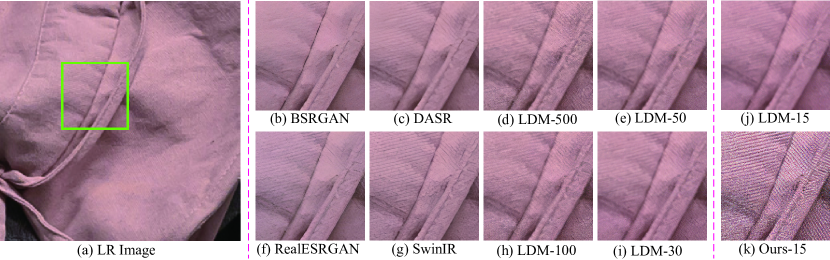
Figure 1: Qualitative comparisons on one typical real-world example of the proposed method and recent state of the arts, including BSRGAN [18], RealESRGAN [19], SwinIR [20], DASR [21], and LDM [11]. As for LDM and our method, we mark the number of sampling steps with the format of “LDM (or Ours)-A” for more intuitive visualization, where “A” is the number of sampling steps. Note that LDM contains 1000 diffusion steps in training and is accelerated to “A” steps using DDIM [16] during inference. Please zoom in for a better view.

Let us revisit the diffusion model in the context of image generation. In the forward process, it builds up a Markov chain to gradually transform the observed data into a pre-specified prior distribution, typically a standard Gaussian distribution, over a large number of steps. Subsequently, image generation can be achieved by sampling a noise map from the prior distribution and feeding it into the reverse path of the Markov chain. While the Gaussian prior is well-suited for the task of image generation, it may not be optimal for SR, where the LR image is available. In this paper, we argue that the reasonable diffusion model for SR should start from a prior distribution based on the LR image, enabling an iterative recovery of the HR image from its LR counterpart instead of Gaussian white noise. Additionally, such a design can reduce the number of diffusion steps required for sampling, thereby improving inference efficiency.

Following the aforementioned motivation, we propose an efficient diffusion model involving a shorter Markov chain for transitioning between the HR image and its corresponding LR one. The initial state of the Markov chain converges to an approximate distribution of the HR image, while the final state converges to an approximate distribution of the LR image. To achieve this, we carefully design a transition kernel that shifts the residual between them step by step. This approach is more efficient than existing diffusion-based SR methods since the residual information can be quickly transferred in dozens of steps. Moreover, our design also allows for an analytical and concise expression for the evidence lower bound, easing the induction of the optimization objective for training. Based on this constructed diffusion kernel, we further develop a highly flexible noise schedule that controls the shifting speed of the residual and the noise strength in each step. This schedule facilitates a fidelity-realism trade-off of the recovered results by tuning its hyper-parameters.

In summary, the main contributions of this work are as follows:

• We present an efficient diffusion model for SR, which renders an iterative sampling procedure from the LR image to the desirable HR one by shifting the residual between them during inference. Extensive experiments demonstrate the superiority of our approach in terms of efficiency, as it requires only 15 sampling steps to achieve appealing results, outperforming or at least being comparable to current diffusion-based SR methods that require a long sampling process. A preview of our recovered results compared with existing methods is shown in Fig. 1.

• We formulate a highly flexible noise schedule for the proposed diffusion model, enabling more precise control of the shifting of residual and noise levels during the transition.

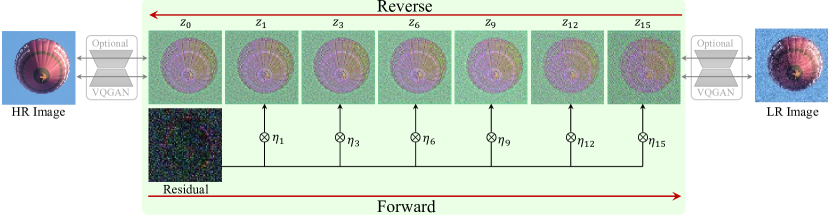
Figure 2: Overview of the proposed method. It builds up a Markov chain between the HR/LR image pair by shifting their residual.

2 Methodology

In this section, we present a diffusion model, ResShift, which is tailored for SR. For ease of presentation, the LR and HR images are denoted as $\bm{y}_{0}$ and $\bm{x}_{0}$, respectively. Furthermore, we assume $\bm{y}_{0}$ and $\bm{x}_{0}$ have identical spatial resolution, which can be easily achieved through pre-upsampling the LR image $\bm{y}_{0}$ using nearest neighbor interpolation if necessary.

2.1 Model Design

The iterative generation paradigm of diffusion models has proven highly effective at capturing complex distributions, inspiring us to approach the SR problem iteratively as well. Our proposed method constructs a Markov chain that serves as a bridge between the HR and LR images as shown in Fig. 2. This way, the SR task can be accomplished by reverse sampling from this Markov chain given any LR image. Next, we will detail the process of building such a Markov chain specifically for SR.

Forward Process. Let’s denote the residual between the LR and HR images as $\bm{e}_{0}$, i.e., $\bm{e}_{0}=\bm{y}_{0}-\bm{x}_{0}$. Our core idea is to transit from $\bm{x}_{0}$ to $\bm{y}_{0}$ by gradually shifting their residual $\bm{e}_{0}$ through a Markov chain with length $T$. A shifting sequence $\{\eta_{t}\}_{t=1}^{T}$ is first introduced, which monotonically increases with the timestep $t$ and satisfies $\eta_{1}\to 0$ and $\eta_{T}\to 1$. The transition distribution is then formulated based on this shifting sequence as follows:

$$q(\bm{x}_{t}|\bm{x}_{t-1},\bm{y}_{0})=\mathcal{N}(\bm{x}_{t};\bm{x}_{t-1}+\alpha_{t}\bm{e}_{0},\kappa^{2}\alpha_{t}\bm{I}),~{}t=1,2,\cdots,T,$$ (1)

where $\alpha_{t}=\eta_{t}-\eta_{t-1}$ for $t>1$ and $\alpha_{1}=\eta_{1}$, $\kappa$ is a hyper-parameter controlling the noise variance, $\bm{I}$ is the identity matrix. Notably, we show that the marginal distribution at any timestep $t$ is analytically integrable, namely

$$q(\bm{x}_{t}|\bm{x}_{0},\bm{y}_{0})=\mathcal{N}(\bm{x}_{t};\bm{x}_{0}+\eta_{t}\bm{e}_{0},\kappa^{2}\eta_{t}\bm{I}),~{}t=1,2,\cdots,T.$$ (2)

The design of the transition distribution presented in Eq. (1) is based on two primary principles. The first principle concerns the standard deviation, i.e., $\kappa\sqrt{\alpha_{t}}$, which aims to facilitate a smooth transition between $\bm{x}_{t}$ and $\bm{x}_{t-1}$. This is because the expected distance between $\bm{x}_{t}$ and $\bm{x}_{t-1}$ can be bounded by $\sqrt{\alpha_{t}}$, given that the image data falls within the range of $[0,1]$, i.e.,

$$\text{max}[(\bm{x}_{0}+\eta_{t}\bm{e}_{0})-(\bm{x}_{0}+\eta_{t-1}\bm{e}_{0})]=\text{max}[\alpha_{t}\bm{e}_{0}]<\alpha_{t}<\sqrt{\alpha_{t}},$$ (3)

where $\text{max}[\cdot]$ represents the pixel-wise maximizing operation. The hyper-parameter $\kappa$ is introduced to increase the flexibility of this design. The second principle pertains to the mean parameter, i.e., $\bm{x}_{0}+\alpha_{t}\bm{e}_{0}$, which induces the marginal distribution in Eq. (2). Furthermore, the marginal distributions of $\bm{x}_{1}$ and $\bm{x}_{T}$ converges to $\delta_{\bm{x}_{0}}(\cdot)$ and $\mathcal{N}(\cdot;\bm{y}_{0},\kappa^{2}\bm{I})$, which act as two approximate distributions for the HR image and the LR image, respectively. By constructing the Markov chain in such a thoughtful way, it is possible to handle the SR task by inversely sampling from it given the LR image $\bm{y}_{0}$.

Reverse Process. The reverse process aims to estimate the posterior distribution $p(\bm{x}_{0}|\bm{y}_{0})$ via the following formulation:

$$p(\bm{x}_{0}|\bm{y}_{0})=\int p(\bm{x}_{T}|\bm{y}_{0})\prod_{t=1}^{T}p_{\bm{\theta}}(\bm{x}_{t-1}|\bm{x}_{t},\bm{y}_{0})\mathrm{d}\bm{x}_{1:T},$$ (4)

where $p(\bm{x}_{T}|\bm{y}_{0})\approx\mathcal{N}(\bm{x}_{T}|\bm{y}_{0},\kappa^{2}\bm{I})$, $p_{\bm{\theta}}(\bm{x}_{t-1}|\bm{x}_{t},\bm{y}_{0})$ is the inverse transition kernel from $\bm{x}_{t}$ to $\bm{x}_{t-1}$ with a learnable parameter $\bm{\theta}$. Following most of the literature in diffusion model [1, 2, 8], we adopt the assumption of $p_{\bm{\theta}}(\bm{x}_{t-1}|\bm{x}_{t},\bm{y}_{0})=\mathcal{N}(\bm{x}_{t-1};\bm{\mu}_{\bm{\theta}}(\bm{x}_{t},\bm{y}_{0},t),\bm{\Sigma}_{\bm{\theta}}(\bm{x}_{t},\bm{y}_{0},t))$. The optimization for $\bm{\theta}$ is achieved by minimizing the negative evidence lower bound, namely,

$$\min_{\bm{\theta}}\sum_{t}D_{\text{KL}}\left[q(\bm{x}_{t-1}|\bm{x}_{t},\bm{x}_{0},\bm{y}_{0})\|p_{\bm{\theta}}(\bm{x}_{t-1}|\bm{x}_{t},\bm{y}_{0})\right],$$ (5)

where $D_{\text{KL}}[\cdot\|\cdot]$ denotes the Kullback-Leibler (KL) divergence. More mathematical details can be found in Sohl-Dickstein et al. [1] or Ho et al. [2].

Combining Eq. (1) and Eq. (2), the targeted distribution $q(\bm{x}_{t-1}|\bm{x}_{t},\bm{x}_{0},\bm{y}_{0})$ in Eq. (5) can be rendered tractable and expressed in an explicit form given below:

$$q(\bm{x}_{t-1}|\bm{x}_{t},\bm{x}_{0},\bm{y}_{0})=\mathcal{N}\left(\bm{x}_{t-1}\bigg{|}\frac{\eta_{t-1}}{\eta_{t}}\bm{x}_{t}+\frac{\alpha_{t}}{\eta_{t}}\bm{x}_{0},\kappa^{2}\frac{\eta_{t-1}}{\eta_{t}}\alpha_{t}\bm{I}\right).$$ (6)

The detailed calculation of this derivation is presented in Appendix A. Considering that the variance parameter is independent of $\bm{x}_{t}$ and $\bm{y}_{0}$, we thus set $\bm{\Sigma}_{\bm{\theta}}(\bm{x}_{t},\bm{y}_{0},t)=\kappa^{2}\frac{\eta_{t-1}}{\eta_{t}}\alpha_{t}\bm{I}$. As for the mean parameter $\bm{\mu}_{\bm{\theta}}(\bm{x}_{t},\bm{y}_{0},t)$, it is reparameterized as follows:

$$\bm{\mu}_{\bm{\theta}}(\bm{x}_{t},\bm{y}_{0},t)=\frac{\eta_{t-1}}{\eta_{t}}\bm{x}_{t}+\frac{\alpha_{t}}{\eta_{t}}f_{\bm{\theta}}(\bm{x}_{t},\bm{y}_{0},t),$$ (7)

where $f_{\bm{\theta}}$ is a deep neural network with parameter $\bm{\theta}$, aiming to predict $\bm{x}_{0}$. We explored different parameterization forms on $\bm{\mu}_{\theta}$ and found that Eq. (7) exhibits superior stability and performance.

Based on Eq. (7), we simplify the objective function in Eq. (5) as follows,

$$\min_{\bm{\theta}}\sum\nolimits_{t}w_{t}\|f_{\bm{\theta}}(\bm{x}_{t},\bm{y}_{0},t)-\bm{x}_{0}\|_{2}^{2},$$ (8)

where $w_{t}=\frac{\alpha_{t}}{2\kappa^{2}\eta_{t}\eta_{t-1}}$. In practice, we empirically find that the omission of weight $w_{t}$ results in an evident improvement in performance, which aligns with the conclusion in Ho et al. [2].

Extension to Latent Space. To alleviate the computational overhead in training, we move the aforementioned model into the latent space of VQGAN [22], where the original image is compressed by a factor of four in spatial dimensions. This does not require any modifications on our model other than substituting $\bm{x_{0}}$ and $\bm{y}_{0}$ with their latent codes. An intuitive illustration is shown in Fig. 2.

2.2 Noise Schedule

The proposed method employs a hyper-parameter $\kappa$ and a shifting sequence $\{\eta_{t}\}_{t=1}^{T}$ to determine the noise schedule in the diffusion process. Specifically, the hyper-parameter $\kappa$ regulates the overall noise intensity during the transition, and its impact on performance is empirically discussed in Sec. 4.2. The subsequent exposition mainly revolves around the construction of the shifting sequence $\{\eta_{t}\}_{t=1}^{T}$.

Equation (2) implies that the noise level in state $\bm{x}_{t}$ is proportional to $\sqrt{\eta_{t}}$ with a scaling factor $\kappa$. This observation motivates us to focus on designing $\sqrt{\eta_{t}}$ instead of $\eta_{t}$. Song and Ermon [23] show that $\kappa\sqrt{\eta_{1}}$ should be sufficiently small (e.g., 0.04 in LDM [11]) to ensure that $q(\bm{x}_{1}|\bm{x}_{0},\bm{y}_{0})\approx q(\bm{x}_{0})$. Combining with the additional constraint of $\eta_{1}\to 0$, we set $\eta_{1}$ to be the minimum value between $(\nicefrac{{0.04}}{{\kappa}})^{2}$ and $0.001$. For the final step $T$, we set $\eta_{T}$ as 0.999 ensuring $\eta_{T}\to 1$. For the intermediate timesteps, i.e., $t\in[2,T-1]$, we propose a non-uniform geometric schedule for $\sqrt{\eta_{t}}$ as follows:

$$\sqrt{\eta_{t}}=\sqrt{\eta_{1}}\times b_{0}^{\beta_{t}},~{}t=2,\cdots,T-1,$$ (9)

where

$$\beta_{t}=\left(\frac{t-1}{T-1}\right)^{p}\times(T-1),~{}b_{0}=\exp\left[\frac{1}{2(T-1)}\log{\frac{\eta_{T}}{\eta_{1}}}\right].$$ (10)

Note that the choice of $\beta_{t}$ and $b_{0}$ is based on the assumption of $\beta_{1}=0$, $\beta_{T}=T-1$, and $\sqrt{\eta_{T}}=\sqrt{\eta_{1}}\times b_{0}^{T-1}$. The hyper-parameter $p$ controls the growth rate of $\sqrt{\eta_{t}}$ as shown in Fig. 3(h).

The proposed noise schedule exhibits high flexibility in three key aspects. First, for small values of $\kappa$, the final state $\bm{x}_{T}$ converges to a perturbation around the LR image as depicted in Fig. 3(c)-(d). Compared to the corruption ended at Gaussian noise, this design considerably shortens the length of the Markov chain, thereby improving the inference efficiency. Second, the hyper-parameter $p$ provides precise control over the shifting speed, enabling a fidelity-realism trade-off in the SR results as analyzed in Sec. 4.2. Third, by setting $\kappa=40$ and $p=0.8$, our method achieves a diffusion process remarkably similar to LDM [11]. This is clearly demonstrated by the visual results during the diffusion process presented in Fig. 3(e)-(f), and further supported by the comparisons on the relative noise strength as shown in Fig. 3(g).

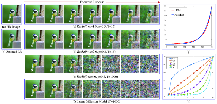
Figure 3: Illustration of the proposed noise schedule. (a) HR image. (b) Zoomed LR image. (c)-(d) Diffused images of ResShift in timesteps of 1, 3, 5, 7, 9, 12, and 15 under different values of $\kappa$ by fixing $p=0.3$ and $T=15$. (e)-(f) Diffused images of ResShift with a specified configuration of $\kappa=40,p=0.8,T=1000$ and LDM [11] in timesteps of 100, 200, 400, 600, 800, 900, and 1000. (g) The relative noise intensity (vertical axes, measured by $\sqrt{\nicefrac{{1}}{{\lambda_{\text{snr}}}}}$, where $\lambda_{\text{snr}}$ denotes the signal-to-noise ratio) of the schedules in (d) and (e) w.r.t. the timesteps (horizontal axes). (h) The shifting speed $\sqrt{\eta_{t}}$ (vertical axes) w.r.t. to the timesteps (horizontal axes) across various configurations of $p$. Note that the diffusion processes in this figure are implemented in the latent space, but we display the intermediate results after decoding back to the image space for the purpose of easy visualization.

3 Related Work

Diffusion Model. Inspired by the non-equilibrium statistical physics, Sohl-Dickstein et al. [1] firstly proposed the diffusion model to fit complex distributions. Ho et al. [2] established a novel connection between the diffusion model and the denoising scoring matching. Later, Song et al. [8] proposed a unified framework to formulate the diffusion model from the perspective of the stochastic differential equation (SDE). Attributed to its robust theoretical foundation, the diffusion model has achieved impressive success in the generation of images [3, 11], audio [24], graph [25] and shapes [26].

Image Super-Resolution. Traditional image SR methods primarily focus on designing more rational image priors based on our subjective knowledge, such as non-local similarity [27], low-rankness [28], sparsity [29, 30], and so on. With the development of deep learning (DL), Dong et al. [31] proposed the seminal work SRCNN to solve the SR task using a deep neural network. Then DL-based SR methods rapidly dominated the research field. Various SR technologies were explored from different perspectives, including network architecture [32, 33, 34, 35], image prior [36, 37, 38, 39], deep unfolding [40, 41, 42], degradation model [43, 18, 19, 44].

Recently, some works have investigated the application of diffusion models in SR. A prevalent approach is to concatenate the LR image with the noise in each step and retrain the diffusion model from scratch [45, 10, 11]. Another popular way is to utilize an unconditional pre-trained diffusion model as a prior and incorporate additional constraints to guide the reverse process [12, 7, 46, 13]. Both strategies often require hundreds or thousands of sampling steps to generate a realistic HR image. While several acceleration algorithms [15, 16, 17] have been proposed, they typically sacrifice the performance and result in blurry outputs. This work designs a more efficient diffusion model that overcomes this trade-off between efficiency and performance, as detailed in Sec. 2.

Remark. Several parallel works [47, 48, 49] also exploit such an iterative restoration paradigm in SR. Despite a similar motivation, our work and others have adopted different mathematical formulations to achieve this goal. Delbracio and Milanfar [47] employed the Inversion by Direct Iteration (InDI) to model this process, while Luo et al. [48] and Liu et al. [49] attempted to formulate it as a SDE. In this paper, we design a discrete Markov chain to depict the transition between the HR and LR images, offering a more intuitive and efficient solution to this problem.

Table 1: Performance comparison of ResShift on the ImageNet-Test under different configurations.

Configurations			Metrics
$T$	$p$	$\kappa$	PSNR$\uparrow$	SSIM$\uparrow$	LPIPS$\downarrow$	CLIPIQA$\uparrow$	MUSIQ$\uparrow$
10	0.3	2.0	25.20	0.6828	0.2517	0.5492	50.6617
15			25.01	0.6769	0.2312	0.5922	53.6596
30			24.52	0.6585	0.2253	0.6273	55.7904
40			24.29	0.6513	0.2225	0.6468	56.8482
50			24.22	0.6483	0.2212	0.6489	56.8463
15	0.3	2.0	25.01	0.6769	0.2312	0.5922	53.6596
	0.5		25.05	0.6745	0.2387	0.5816	52.4475
	1.0		25.12	0.6780	0.2613	0.5314	48.4964
	2.0		25.32	0.6827	0.3050	0.4601	43.3060
	3.0		25.39	0.5813	0.3432	0.4041	38.5324
15	0.3	0.5	24.90	0.6709	0.2437	0.5700	50.6101
		1.0	24.84	0.6699	0.2354	0.5914	52.9933
		2.0	25.01	0.6769	0.2312	0.5922	53.6596
		8.0	25.31	0.6858	0.2592	0.5231	49.3182
		16.0	24.46	0.6891	0.2772	0.4898	46.9794

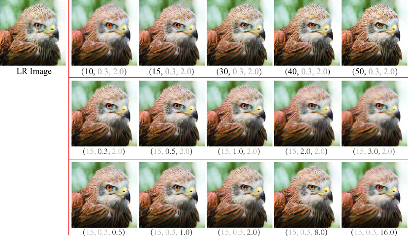
Figure 4: Qualitative comparisons of ResShift under different combinations of ($T$, $p$, $\kappa$). For example, “(15, 0.3, 2.0)” represents the recovered result with $T=15$, $p=0.3$, and $\kappa=2.0$. Please zoom in for a better view.

4 Experiments

This section presents an empirical analysis of the proposed ResShift and provides extensive experimental results to verify its effectiveness on one synthetic dataset and three real-world datasets. Following [18, 19], our investigation specifically focuses on the more challenging $\times 4$ SR task. Due to page limitation, some experimental results are put in the Appendix B.

4.1 Experimental Setup

Training Details. HR images with a resolution of $256\times 256$ in our training data are randomly cropped from the training set of ImageNet [50] following LDM [11]. We synthesize the LR images using the degradation pipeline of RealESRGAN [19]. The Adam [51] algorithm with the default settings of PyTorch [52] and a mini-batch size of 64 is used to train ResShift. During training, we use a fixed learning rate of $5\text{e-}5$ and update the weight parameters for 500K iterations. As for the network architecture, we employ the UNet structure in DDPM [2]. To increase the robustness of ResShift to arbitrary image resolution, we replace the self-attention layer in UNet with the Swin Transformer [53] block.

Testing Datasets. We synthesize a testing dataset that contains 3000 images randomly selected from the validation set of ImageNet [50] based on the commonly-used degradation model, i.e., $\bm{y}=(\bm{x}*\bm{k})\downarrow+\bm{n}$, where $k$ is the blurring kernel, $n$ is the noise, $\bm{y}$ and $\bm{x}$ denote the LR image and HR image, respectively. To comprehensively evaluate the performance of ResShift, we consider more complicated types of blurring kernels, downsampling operators, and noise types. The detailed settings on them can be found in Appendix B.1. It should be noted that we selected the HR images from ImageNet [50] instead of the prevailing datasets in SR such as Set5 [54], Set14 [55], and Urban100 [56]. The rationale behind this setting is rooted in the fact that these datasets only contain very few source images, which fails to thoroughly evaluate the performance of various methods under different degradation types. We name this dataset as ImageNet-Test for convenience.

Two real-world datasets are adopted to evaluate the efficacy of ResShift. The first is RealSR [57], containing 100 real images captured by Canon 5D3 and Nikon D810 cameras. Additionally, we collect another real-world dataset named RealSet65. It comprises 35 LR images widely used in recent literature [58, 59, 60, 61, 19]. The remaining 30 images were obtained from the internet by ourselves.

Compared Methods. We evaluate the effectiveness of ResShift in comparison to seven recent SR methods, namely ESRGAN [62], RealSR-JPEG [63], BSRGAN [18], RealESRGAN [19], SwinIR [20], DASR [21], and LDM [11]. Note that LDM is a diffusion-based method with 1,000 diffusion steps. For a fair comparison, we accelerate LDM to the same number of steps with ResShift using DDIM [16] and denote it as “LDM-A", where “A" indicates the number of inference steps. The hyper-parameter $\eta$ in DDIM is set to be 1 as this value yields the most realistic recovered images.

Metrics. The performance of various methods was assessed using five metrics, including PSNR, SSIM [64], LPIPS [65], MUSIQ [66], and CLIPIQA [67]. It is worth noting that the latter two are non-reference metrics specifically designed to assess the realism of images. CLIPIQA, in particular, leverages the CLIP [68] model that is pre-trained on a massive dataset (i.e., Laion400M [69]) and thus demonstrates strong generalization ability. On the real-world datasets, we mainly rely on CLIPIQA and MUSIQ as evaluation metrics to compare the performance of different methods.

Table 2: Efficiency and performance comparisons of ResShift to other methods on the dataset of ImageNet-Test. “LDM-A” represents the results achieved by accelerated the sampling steps of LDM [11] to “A”. Running time is tested on NVIDIA Tesla V100 GPU on the x4 (64$\rightarrow$ 256) SR task.

Metrics	Methods
8
	BSRGAN	RealESRGAN	SwinIR	LDM-15	LDM-30	LDM-100	ResShift
PSNR$\uparrow$	24.42	24.04	23.99	24.89	24.49	23.90	25.01
LPIPS$\downarrow$	0.259	0.254	0.238	0.269	0.248	0.244	0.231
CLIPIQA$\uparrow$	0.581	0.523	0.564	0.512	0.572	0.620	0.592
Runtime (s)	0.012	0.013	0.046	0.102	0.184	0.413	0.105
# Parameters (M)	16.70	16.70	28.01	113.60			118.59

4.2 Model Analysis

We analyze the performance of ResShift under different settings on the number of diffusion steps $T$ and the hyper-parameters $p$ in Eq. (10) and $\kappa$ in Eq. (1).

Diffusion Steps $T$ and Hyper-parameter $p$. The proposed transition distribution in Eq. (1) significantly reduces the diffusion steps $T$ in the Markov chain. The hyper-parameter $p$ allows for flexible control over the speed of residual shifting during the transition. Table 1 summarizes the performance of ResShift on ImageNet-Test under different configurations of $T$ and $p$. We can see that both of $T$ and $p$ render a trade-off between the fidelity, measured by the reference metrics such as PSNR, SSIM, and LPIPS, and the realism, measured by the non-reference metrics, including CLIPIQA and MUSIQ, of the super-resolved results. Taking $p$ as an example, when it increases, the reference metrics improve while the non-reference metrics deteriorate. Furthermore, the visual comparison in Fig. 4 shows that a large value of $p$ will suppress the model’s ability to hallucinate more image details and result in blurry outputs.

Table 3: Quantitative results of different methods on the dataset of ImageNet-Test. The best and second best results are highlighted in bold and underline.

Methods	Metrics
6
	PSNR$\uparrow$	SSIM$\uparrow$	LPIPS$\downarrow$	CLIPIQA$\uparrow$	MUSIQ$\uparrow$
ESRGAN [62]	20.67	0.448	0.485	0.451	43.615
RealSR-JPEG [63]	23.11	0.591	0.326	0.537	46.981
BSRGAN [18]	24.42	0.659	0.259	0.581	54.697
SwinIR [20]	23.99	0.667	0.238	0.564	53.790
RealESRGAN [19]	24.04	0.665	0.254	0.523	52.538
DASR [21]	24.75	0.675	0.250	0.536	48.337
LDM-15 [11]	24.89	0.670	0.269	0.512	46.419
ResShift	25.01	0.677	0.231	0.592	53.660

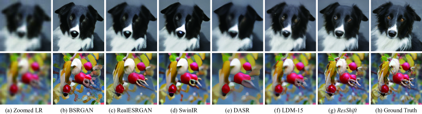
Figure 5: Qualitative comparisons of different methods on two synthetic examples of the ImageNet-Test dataset. Please zoom in for a better view.

Hyper-parameter $\kappa$. Equation (2) reveals that $\kappa$ dominates the noise strength in state $\bm{x}_{t}$. We report the influence of $\kappa$ to the performance of ResShift in Table 1. Combining with the visualization in Fig. 4, we can find that excessively large or small values of $\kappa$ will smooth the recovered results, regardless of their favorable metrics of PSNR and SSIM. When $\kappa$ is in the range of $[1.0,2.0]$, our method achieves the most realistic quality indicated by CLIPIQA and MUSIQ, which is more desirable in real applications. We thus set $\kappa$ to be $2.0$ in this work.

Table 4: Quantitative results of different methods on two real-world datasets. The best and second best results are highlighted in bold and underline.

Methods	Datasets
5
	RealSR		RealSet65
5
	CLIPIQA$\uparrow$	MUSIQ$\uparrow$	CLIPIQA$\uparrow$	MUSIQ$\uparrow$
ESRGAN [62]	0.2362	29.048	0.3739	42.369
RealSR-JPEG [63]	0.3615	36.076	0.5282	50.539
BSRGAN [18]	0.5439	63.586	0.6163	65.582
SwinIR [20]	0.4654	59.636	0.5782	63.822
RealESRGAN [19]	0.4898	59.678	0.5995	63.220
DASR [21]	0.3629	45.825	0.4965	55.708
LDM-15 [11]	0.3836	49.317	0.4274	47.488
ResShift	0.5958	59.873	0.6537	61.330

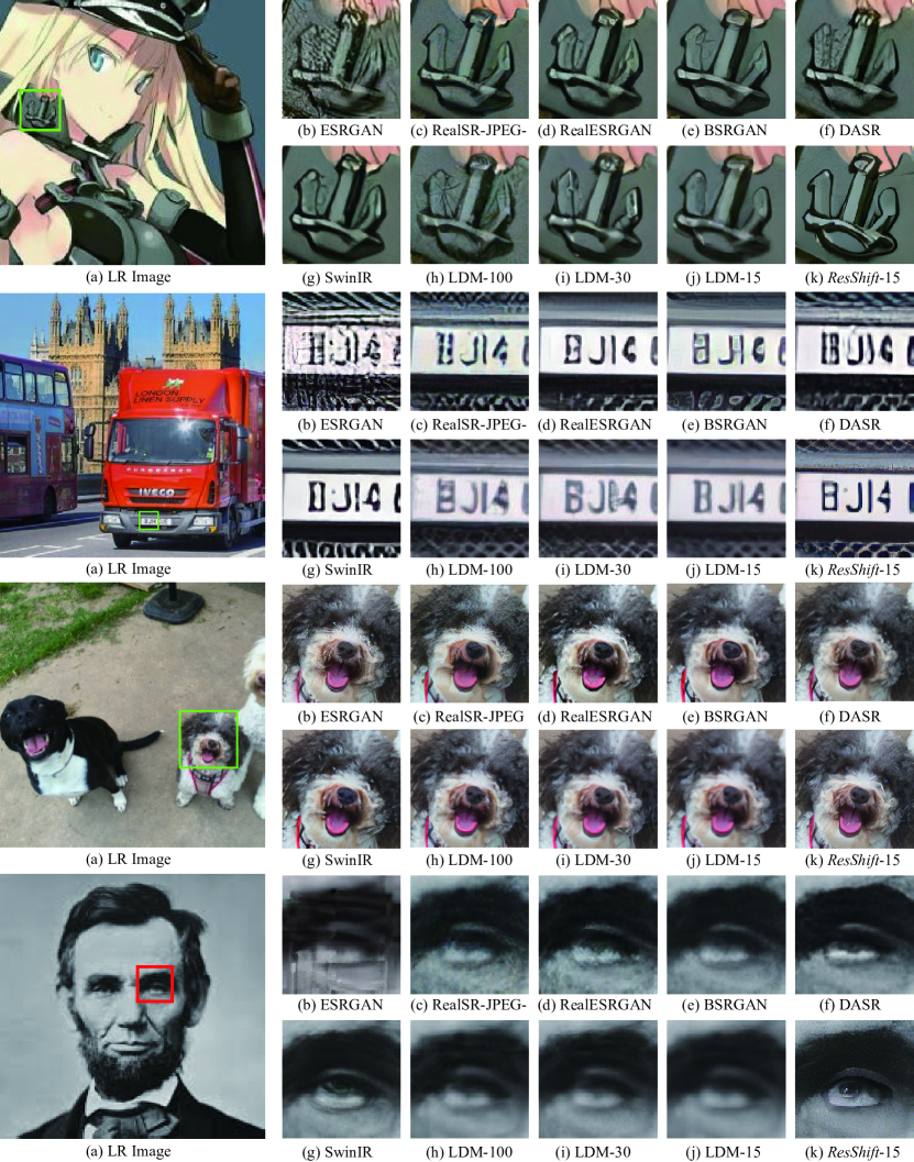
Figure 6: Qualitative comparisons on four real-world examples. Please zoom in for a better view.

Efficiency Comparison. To improve inference efficiency, it is desirable to limit the number of diffusion steps $T$. However, this causes a decrease in the realism of the restored HR images. To compromise, the hyper-parameter $p$ can be set to a relatively small value. Therefore, we set $T=15$ and $p=0.3$, and yield our model named ResShift. Table 2 presents the efficiency and performance comparisons of ResShift to the state-of-the-art (SotA) approach LDM [11] and three other GAN-based methodologies on ImageNet-Test dataset. It is evident from the results that the proposed ResShift surpasses LDM [11] in terms of PSNR and LPIPS [65], and demonstrates a remarkable fourfold enhancement in computational efficiency when compared to LDM-100. Despite showing considerable potential in mitigating the efficiency bottleneck of the diffusion-based SR approaches, ResShift still lags behind current GAN-based methods in speed due to its iterative sampling mechanism.

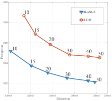
Figure 7: Perception-distortion trade-off of ResShift and LDM. The vertical and horizontal axes represent the strength of the perception and distortion, measured by LPIPS and MSE, respectively.

Therefore, it remains imperative to explore further optimizations of the proposed method to address this limitation, which we leave in our future work.

Perception-Distortion Trade-off. There exists a well-known phenomenon called perception-distortion trade-off [70] in the field of SR. In particular, the augmentation of the generative capability of a restoration model, such as elevating the sampling steps for a diffusion-based method or amplifying the weight of the adversarial loss for a GAN-based method, will result in a deterioration in fidelity preservation while concurrently enhancing the authenticity of restored images. That is mainly because the restoration model with powerful generation capability tends to hallucinate more high-frequency image structures, thereby deviating from the underlying ground truth. To facilitate a comprehensive comparison between our ResShift and current SotA diffusion-based method LDM, we plotted the perception-distortion curves of them in Fig. 7, wherein the perception and distortion are measured by LPIPS and mean square-error (MSE), respectively. This plot reflects the perception quality and the reconstruction fidelity of ResShift and LDM across varying numbers of diffusion steps, i.e., 10, 15, 20, 30, 40, and 50. As can be observed, the perception-distortion curve of our ResShift consistently resides beneath that of the LDM, indicating its superior capacity in balancing perception and distortion.

4.3 Evaluation on Synthetic Data

We present a comparative analysis of the proposed method with recent SotA approaches on the ImageNet-Test dataset, as summarized in Table 3 and Fig. 5. Based on this evaluation, several significant conclusions can be drawn as follows: i) ResShift exhibits superior or at least comparable performance across all five metrics, affirming the effectiveness and superiority of the proposed method. ii) The notably higher PSNR ans SSIM values attained by ResShift indicate its capacity to better preserve fidelity to ground truth images. This advantage primarily arises from our well-designed diffusion model, which starts from a subtle disturbance of the LR image, rather than the conventional assumption of white Gaussian noise in LDM. iii) Considering the metrics of LPIPS and CLIPIQA, which gauge the perceptual quality and realism of the recovered image, ResShift also demonstrates evident superiority over existing methods. Furthermore, in terms of MUSIQ, our approach achieves comparable performance with recent SotA methods. In summary, the proposed ResShift exhibits remarkable capabilities in generating more realistic results while preserving fidelity. This is of paramount importance for the task of SR.

4.4 Evaluation on Real-World Data

Table 4 lists the comparative evaluation using CLIPIQA [67] and MUSIQ [66] of various methods on two real-world datasets. Note that CLIPIQA, benefiting from the powerful representative capability inherited from CLIP, performs stably and robustly in assessing the perceptional quality of natural images. The results in Table 4 show that the proposed ResShift evidently surpasses existing methods in CLIPIQA, meaning that the restored outputs of ResShift better align with human visual and perceptive systems. In the case of MUSIQ evaluation, ResShift achieves the competitive performance when compared to current SotA methods, namely BSRGAN [18], SwinIR [20], and RealESRGAN [19]. Collectively, our method shows promising capability in addressing the real-world SR problem.

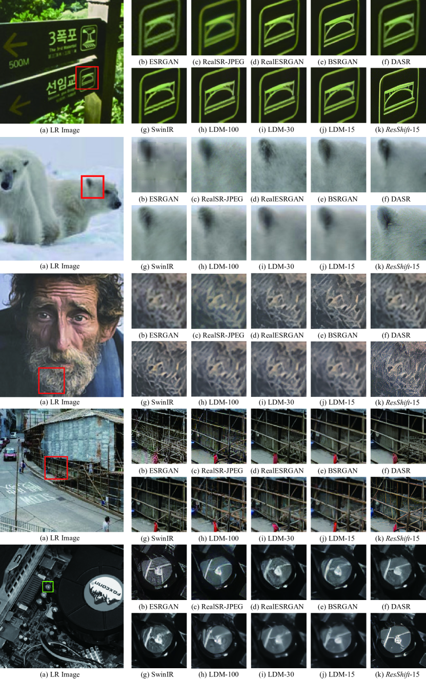
Figure 10: Qualitative comparisons of different methods on real-world datasets. Please zoom in for a better view.

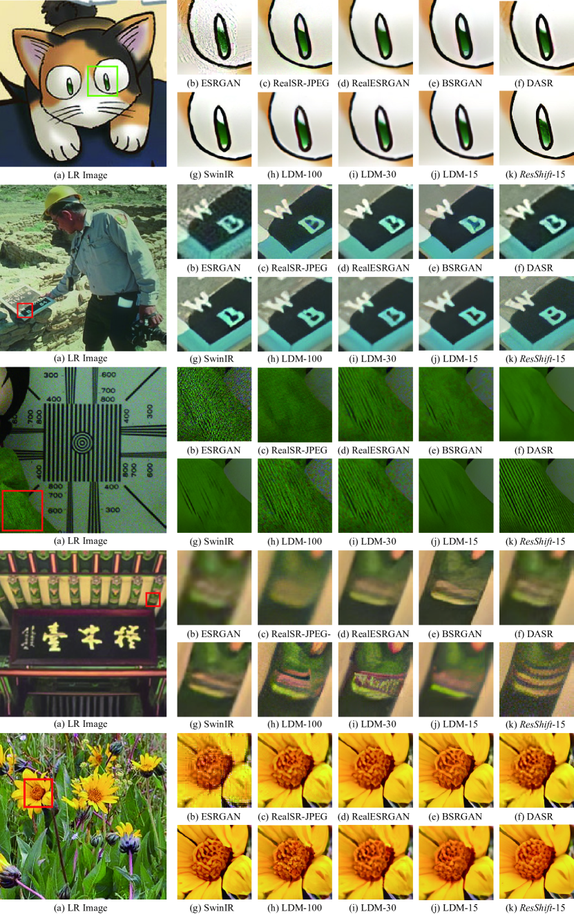
Figure 11: Qualitative comparisons of different methods on real-world datasets. Please zoom in for a better view.

We display four real-world examples in Fig. 6. More examples can be found in Fig. 10 and Fig. 11 of the Appendix. We consider diverse scenarios, including comic, text, face, and natural images to ensure a comprehensive evaluation. A noticeable observation is that ResShift produces more naturalistic image structures, as evidenced by the patterns on the beam in the third example and the eyes of a person in the fourth example. We note that the recovered results of LDM are excessively smooth when compressing the inference steps to match with the proposed ResShift, specifically utilizing 15 steps, largely deviating from the training procedure’s 1,000 steps. Even though other GAN-based methods may also succeed in hallucinating plausible structures to some extent, they are often accompanied by obvious artifacts.

5 Conclusion

In this work, we have introduced an efficient diffusion model named ResShift for SR. Unlike existing diffusion-based SR methods that require a large number of iterations to achieve satisfactory results, our proposed method constructs a diffusion model with only 15 sampling steps, thereby significantly improving inference efficiency. The core idea is to corrupt the HR image toward the LR image instead of the Gaussian white noise, which can effectively cut off the length of the diffusion model. Extensive experiments on both synthetic and real-world datasets have demonstrated the superiority of our proposed method. We believe that our work will pave the way for the development of more efficient and effective diffusion models to address the SR problem.

Acknowledgement. This study is supported under the RIE2020 Industry Alignment Fund – Industry Collaboration Projects (IAF-ICP) Funding Initiative, as well as cash and in-kind contribution from the industry partner(s).

Appendix A Mathematical Details

• Derivation of Eq. (2): According to the transition distribution of Eq. (1), $\bm{x}_{t}$ can be sampled via the following reparameterization trick:

  $$\bm{x}_{t}=\bm{x}_{t-1}+\alpha_{t}\bm{e}_{0}+\kappa\sqrt{\alpha_{t}}\bm{\xi}_{t},$$ (11)

  where $\bm{\xi}_{t}\sim\mathcal{N}(\bm{x}|0,\bm{I})$, $\alpha_{t}=\eta_{t}-\eta_{t-1}$ for $t>1$ and $\alpha_{1}=\eta_{1}$.

  Applying this sampling trick recursively, we can build up the relation between $\bm{x}_{t}$ and $\bm{x}_{0}$ as follows:

  $$\bm{x}_{t} =\bm{x}_{0}+\sum_{i=1}^{t}\alpha_{i}\bm{e}_{0}+\kappa\sum_{i=1}^{t}\sqrt{\alpha_{i}}\bm{\xi}_{i}$$

  $$=\bm{x}_{0}+\eta_{t}\bm{e}_{0}+\kappa\sum_{i=1}^{t}\sqrt{\alpha_{i}}\bm{\xi}_{i},$$ (12)

  where $\bm{\xi}_{i}\sim\mathcal{N}(\bm{x}|0,\bm{I})$.

  We can further merge $\bm{\xi}_{1},\bm{\xi}_{2},\cdots,\bm{\xi}_{t}$ and simplify Eq. (12) as follows:

  $$\bm{x}_{t}=\bm{x}_{0}+\eta_{t}\bm{e}_{0}+\kappa\sqrt{\eta_{t}}\bm{\xi}_{t}.$$ (13)

  Then the marginal distribution of Eq. (2) is obtained based on Eq. (13).

• Derivation of Eq. (6): According to Bayes’s theorem, we have

  $$q(\bm{x}_{t-1}|\bm{x}_{t},\bm{x}_{0},\bm{y}_{0})\propto q(\bm{x}_{t}|\bm{x}_{t-1},\bm{y}_{0})q(\bm{x_{t-1}}|\bm{x}_{0},\bm{y}_{0}),$$ (14)

  where

  $$q(\bm{x}_{t}|\bm{x}_{t-1},\bm{y}_{0})=\mathcal{N}(\bm{x}_{t};\bm{x}_{t-1}+\alpha_{t}\bm{e}_{0},\kappa^{2}\alpha_{t}\bm{I}),$$

  $$q(\bm{x_{t-1}}|\bm{x}_{0},\bm{y}_{0})=\mathcal{N}(\bm{x}_{t-1};\bm{x}_{0}+\eta_{t-1}\bm{e}_{0},\kappa^{2}\eta_{t-1}\bm{I}).$$ (15)

  We now focus on the quadratic form in the exponent of $q(\bm{x}_{t-1}|\bm{x}_{t},\bm{x}_{0},\bm{y}_{0})$, namely,

  $$\mathrel{\phantom{=}}-\frac{(\bm{x}_{t}-\bm{x}_{t-1}-\alpha_{t}\bm{e}_{0})(\bm{x}_{t}-\bm{x}_{t-1}-\alpha_{t}\bm{e}_{0})^{T}}{2\kappa^{2}\alpha_{t}}-\frac{(\bm{x}_{t-1}-\bm{x}_{0}-\eta_{t-1}\bm{e}_{0})(\bm{x}_{t-1}-\bm{x}_{0}-\eta_{t-1}\bm{e}_{0})^{T}}{2\kappa^{2}\eta_{t-1}}$$

  $$=-\frac{1}{2}\left[\frac{1}{\kappa^{2}\alpha_{t}}+\frac{1}{\kappa^{2}\eta_{t-1}}\right]\bm{x}_{t-1}\bm{x}_{t-1}^{T}+\left[\frac{\bm{x}_{t}-\alpha_{t}\bm{e}_{0}}{\kappa^{2}\alpha_{t}}+\frac{\bm{x}_{0}+\eta_{t-1}\bm{e}_{0}}{\kappa^{2}\eta_{t-1}}\right]\bm{x}_{t-1}^{T}+\text{const}$$

  $$=-\frac{(\bm{x}_{t-1}-\bm{\mu})(\bm{x}_{t-1}-\bm{\mu})^{T}}{2\lambda^{2}}+\text{const}$$ (16)

  where

  $$\bm{\mu}=\frac{\eta_{t-1}}{\eta_{t}}\bm{x}_{t}+\frac{\alpha_{t}}{\eta_{t}}\bm{x}_{0},~{}\lambda^{2}=\kappa^{2}\frac{\eta_{t-1}}{\eta_{t}}\alpha_{t},$$ (17)

  and const denotes the item that is independent of $\bm{x}_{t-1}$. This quadratic form induces the Gaussian distribution of Eq. (6).

Appendix B Experiment

B.1 Degradation Settings of the Synthetic Dataset

We synthesize the testing dataset ImageNet-Test based on the degradation model in RealESRGAN [19] but removing the second-order operation. We observed that the LR image generated by the pipeline with second-order degradation exhibited significantly more pronounced corruption than most of the real-world LR images, we thus discarded the second-order operation to align the authentic degradation better. Next, we gave the detailed configuration on the blurring kernel, downsampling operator, and noise types.

Table 5: Quantitative comparison of different methods on the task of x4 (64$\rightarrow$256) bicubic SR . We mark the number of sampling steps for each method by the format of “method-steps”.

Methods	PSNR$\uparrow$	SSIM$\uparrow$	LPIPS$\downarrow$	CLIPIQA$\uparrow$	MUSIQ$\uparrow$	# Parameters (M)	Runtime (s)
IRSDE-100 [48]	24.48	0.602	0.304	0.513	45.382	137.2	5.927
DDRM-15 [46]	25.56	0.674	0.471	0.372	24.746	552.8	1.184
I2SB-15 [49]	26.76	0.730	0.206	0.489	53.936	552.8	1.832
ResShift-15	26.73	0.736	0.126	0.683	58.067	121.3	0.105

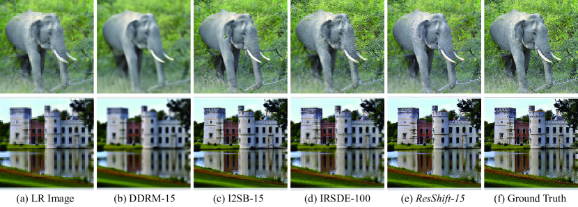
Figure 8: Visual comparisons of different methods on the task of x4 (64$\rightarrow$256) bicubic super-resolution. Please zoom in for a better view.

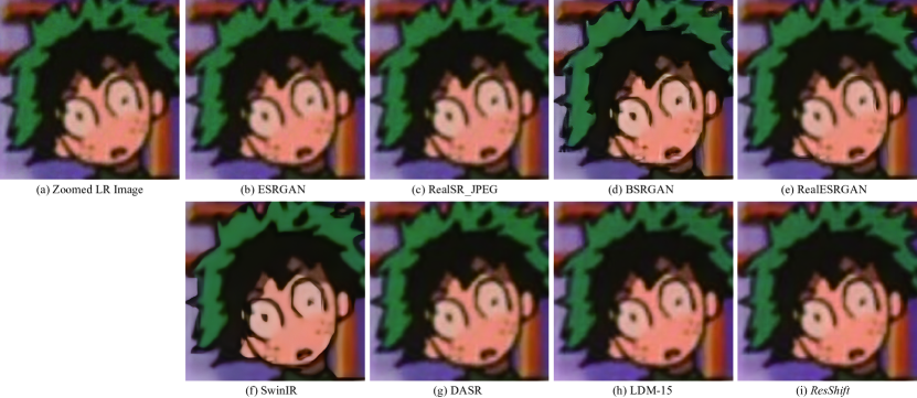
Figure 9: One typical failed case in the real-world dataset of RealSet65.

Blurring kernel. The blurring kernel is randomly sampled from the isotropic Gaussian and anisotropic Gaussian kernels with a probability of [0.6, 0.4]. The window size of the kernel is set to 13. For isotropic Gaussian kernel, the kernel width is uniformly sampled from [0.2, 0.8]. For an anisotropic Gaussian kernel, the kernel widths along $x$-axis and $y$-axis are both randomly sampled from [0.2, 0.8].

Downampling. We downsample the image using the “interpolate” function of PyTorch [52]. The interpolation mode is random selected from “area”, “bilinear”, and “bicubic”.

Noise. We first added Gaussian and Poisson noise with a probability of [0.5, 0.5]. For Gaussian noise, the noise level is randomly chosen from [1,15]. For Poisson noise, we set the scale parameter in [0.05, 0.3]. Finally, the noisy image is further compressed using JPEG with a quality factor ranged in [70, 95].

B.2 Evaluation on Bicubic Degradation

In this section, we conduct an evaluation of the proposed ResShift on the task of x4 (64$\rightarrow$256) bicubic SR, against three recent diffusion-based methods, including DDRM [46], IRSDE [48], and I2SB [49]. To ensure a fair comparison, we retrain a new model specifically tailored for bicubic degradation, given that all three comparison methods were originally designed or trained under the same degradation setting. Our testing dataset comprises 3,000 images randomly selected from the validation dataset of ImageNet [50]. During the evaluation phase, we expedite the inference process to 15 steps using the default sampler for both I2SB and DDRM. However, it is worth noting that we retained the sampling steps of 100 for IRSDE, consistent with its configuration in training, since we empirically found that accelerating the inference of IRSDE led to a severe performance drop.

The quantitative comparison results are listed in Table 5, revealing a conspicuous superiority of our proposed ResShift beyond the alternative methods across various assessment metrics, parameter counts, and inference throughput. This performance difference underscores the effectiveness and efficiency of the proposed diffusion model. The visual comparison of two exemplar cases is depicted in Fig. 8. Our approach demonstrates superior capability in recovering rich and realistic image details, consistent with the quantitative observations.

B.3 Limitation

Albeit its overall strong performance, the proposed ResShift occasionally exhibits failures. One such instance is illustrated in Figure 9, where it cannot produce satisfactory results for a severely degraded comic image. It should be noted that other comparison methods also struggle to address this particular example. This is not an unexpected outcome as most modern SR methods are trained on synthetic datasets simulated by manually assumed degradation models [18, 19], which still cannot cover the full range of complicated real degradation types. Therefore, developing a more practical degradation model for SR is an essential avenue for future research.

References

- Sohl-Dickstein et al. [2015] Jascha Sohl-Dickstein, Eric Weiss, Niru Maheswaranathan, and Surya Ganguli. Deep unsupervised learning using nonequilibrium thermodynamics. In International Conference on Machine Learning (ICML), pages 2256–2265. PMLR, 2015.
- Ho et al. [2020] Jonathan Ho, Ajay Jain, and Pieter Abbeel. Denoising diffusion probabilistic models. In Proceedings of Advances in Neural Information Processing Systems (NeurIPS), volume 33, pages 6840–6851, 2020.
- Dhariwal and Nichol [2021] Prafulla Dhariwal and Alexander Nichol. Diffusion models beat gans on image synthesis. In Proceedings of Advances in Neural Information Processing Systems (NeurIPS), volume 34, pages 8780–8794, 2021.
- Meng et al. [2021] Chenlin Meng, Yutong He, Yang Song, Jiaming Song, Jiajun Wu, Jun-Yan Zhu, and Stefano Ermon. Sdedit: Guided image synthesis and editing with stochastic differential equations. In Proceedings of International Conference on Learning Representations (ICLR), 2021.
- Avrahami et al. [2022] Omri Avrahami, Dani Lischinski, and Ohad Fried. Blended diffusion for text-driven editing of natural images. In Proceedings of the IEEE/CVF Conference on Computer Vision and Pattern Recognition (CVPR), pages 18208–18218, 2022.
- Lugmayr et al. [2022] Andreas Lugmayr, Martin Danelljan, Andres Romero, Fisher Yu, Radu Timofte, and Luc Van Gool. Repaint: Inpainting using denoising diffusion probabilistic models. In Proceedings of the IEEE/CVF Conference on Computer Vision and Pattern Recognition (CVPR), pages 11461–11471, June 2022.
- Chung et al. [2022] Hyungjin Chung, Byeongsu Sim, and Jong Chul Ye. Come-closer-diffuse-faster: Accelerating conditional diffusion models for inverse problems through stochastic contraction. In Proceedings of the IEEE/CVF Conference on Computer Vision and Pattern Recognition (CVPR), pages 12413–12422, 2022.
- Song et al. [2021a] Yang Song, Jascha Sohl-Dickstein, Diederik P Kingma, Abhishek Kumar, Stefano Ermon, and Ben Poole. Score-based generative modeling through stochastic differential equations. In Proceedings of International Conference on Learning Representations (ICLR), 2021a.
- Saharia et al. [2022a] Chitwan Saharia, William Chan, Huiwen Chang, Chris Lee, Jonathan Ho, Tim Salimans, David Fleet, and Mohammad Norouzi. Palette: Image-to-image diffusion models. In Proceedings of ACM SIGGRAPH Conference, pages 1–10, 2022a.
- Saharia et al. [2022b] Chitwan Saharia, Jonathan Ho, William Chan, Tim Salimans, David J Fleet, and Mohammad Norouzi. Image super-resolution via iterative refinement. IEEE Transactions on Pattern Analysis and Machine Intelligence (TPAMI), 2022b.
- Rombach et al. [2022] Robin Rombach, Andreas Blattmann, Dominik Lorenz, Patrick Esser, and Björn Ommer. High-resolution image synthesis with latent diffusion models. In Proceedings of the IEEE/CVF Conference on Computer Vision and Pattern Recognition (CVPR), pages 10684–10695, 2022.
- Choi et al. [2021] Jooyoung Choi, Sungwon Kim, Yonghyun Jeong, Youngjune Gwon, and Sungroh Yoon. Ilvr: Conditioning method for denoising diffusion probabilistic models. In Proceedings of the IEEE/CVF International Conference on Computer Vision (ICCV), pages 14367–14376, 2021.
- Yue and Loy [2022] Zongsheng Yue and Chen Change Loy. Difface: Blind face restoration with diffused error contraction. arXiv preprint arXiv:2212.06512, 2022.
- Wang et al. [2023a] Jianyi Wang, Zongsheng Yue, Shangchen Zhou, Kelvin C.K. Chan, and Chen Change Loy. Exploiting diffusion prior for real-world image super-resolution. arXiv preprint arXiv:2305.07015, 2023a.
- Nichol and Dhariwal [2021] Alexander Quinn Nichol and Prafulla Dhariwal. Improved denoising diffusion probabilistic models. In International Conference on Machine Learning (ICML), pages 8162–8171. PMLR, 2021.
- Song et al. [2021b] Jiaming Song, Chenlin Meng, and Stefano Ermon. Denoising diffusion implicit models. In Proceedings of International Conference on Learning Representations (ICLR), 2021b.
- Lu et al. [2022] Cheng Lu, Yuhao Zhou, Fan Bao, Jianfei Chen, Chongxuan Li, and Jun Zhu. DPM-solver: A fast ODE solver for diffusion probabilistic model sampling in around 10 steps. In Proceedings of Advances in Neural Information Processing Systems (NeurIPS), 2022.
- Zhang et al. [2021] Kai Zhang, Jingyun Liang, Luc Van Gool, and Radu Timofte. Designing a practical degradation model for deep blind image super-resolution. In Proceedings of the IEEE/CVF International Conference on Computer Vision (ICCV), pages 4791–4800, 2021.
- Wang et al. [2021] Xintao Wang, Liangbin Xie, Chao Dong, and Ying Shan. Real-esrgan: Training real-world blind super-resolution with pure synthetic data. In Proceedings of the IEEE/CVF International Conference on Computer Vision Workshops (ICCV-W), pages 1905–1914, 2021.
- Liang et al. [2021a] Jingyun Liang, Jiezhang Cao, Guolei Sun, Kai Zhang, Luc Van Gool, and Radu Timofte. Swinir: Image restoration using swin transformer. In Proceedings of the IEEE/CVF International Conference on Computer Vision Workshops (ICCV-W), pages 1833–1844, 2021a.
- Liang et al. [2022] Jie Liang, Hui Zeng, and Lei Zhang. Efficient and degradation-adaptive network for real-world image super-resolution. In Proceedings of the European Conference on Computer Vision (ECCV), pages 574–591, 2022.
- Esser et al. [2021] Patrick Esser, Robin Rombach, and Bjorn Ommer. Taming transformers for high-resolution image synthesis. In Proceedings of the IEEE/CVF Conference on Computer Vision and Pattern Recognition (CVPR), pages 12873–12883, 2021.
- Song and Ermon [2019] Yang Song and Stefano Ermon. Generative modeling by estimating gradients of the data distribution. In Proceedings of Advances in Neural Information Processing Systems (NeurIPS), volume 32, 2019.
- Chen et al. [2020] Nanxin Chen, Yu Zhang, Heiga Zen, Ron J Weiss, Mohammad Norouzi, and William Chan. WaveGrad: estimating gradients for waveform generation. In Proceedings of International Conference on Learning Representations (ICLR), 2020.
- Niu et al. [2020] Chenhao Niu, Yang Song, Jiaming Song, Shengjia Zhao, Aditya Grover, and Stefano Ermon. Permutation invariant graph generation via score-based generative modeling. In Proceedings of the International Conference on Artificial Intelligence and Statistics (AISTATS), volume 108, pages 4474–4484, 2020.
- Cai et al. [2020] Ruojin Cai, Guandao Yang, Hadar Averbuch-Elor, Zekun Hao, Serge Belongie, Noah Snavely, and Bharath Hariharan. Learning gradient fields for shape generation. In Proceedings of the European Conference on Computer Vision (ECCV), pages 364–381, 2020.
- Dong et al. [2012] Weisheng Dong, Lei Zhang, Guangming Shi, and Xin Li. Nonlocally centralized sparse representation for image restoration. IEEE Transactions on Image Processing (TIP), 22(4):1620–1630, 2012.
- Gu et al. [2017] Shuhang Gu, Qi Xie, Deyu Meng, Wangmeng Zuo, Xiangchu Feng, and Lei Zhang. Weighted nuclear norm minimization and its applications to low level vision. International Journal of Computer Vision (IJCV), 121:183–208, 2017.
- Dong et al. [2011] Weisheng Dong, Lei Zhang, Guangming Shi, and Xiaolin Wu. Image deblurring and super-resolution by adaptive sparse domain selection and adaptive regularization. IEEE Transactions on Image Processing (TIP), 20(7):1838–1857, 2011.
- Gu et al. [2015] Shuhang Gu, Wangmeng Zuo, Qi Xie, Deyu Meng, Xiangchu Feng, and Lei Zhang. Convolutional sparse coding for image super-resolution. In Proceedings of the IEEE/CVF International Conference on Computer Vision (ICCV), pages 1823–1831, 2015.
- Dong et al. [2015] Chao Dong, Chen Change Loy, Kaiming He, and Xiaoou Tang. Image super-resolution using deep convolutional networks. IEEE Transactions on Pattern Analysis and Machine Intelligence (TPAMI), 38(2):295–307, 2015.
- Shi et al. [2016] Wenzhe Shi, Jose Caballero, Ferenc Huszár, Johannes Totz, Andrew P Aitken, Rob Bishop, Daniel Rueckert, and Zehan Wang. Real-time single image and video super-resolution using an efficient sub-pixel convolutional neural network. In Proceedings of the IEEE/CVF Conference on Computer Vision and Pattern Recognition (CVPR), pages 1874–1883, 2016.
- Zhang et al. [2017] Kai Zhang, Wangmeng Zuo, Yunjin Chen, Deyu Meng, and Lei Zhang. Beyond a gaussian denoiser: Residual learning of deep cnn for image denoising. IEEE Transactions on Image Processing (TIP), 26(7):3142–3155, 2017.
- Lai et al. [2017] Wei-Sheng Lai, Jia-Bin Huang, Narendra Ahuja, and Ming-Hsuan Yang. Deep laplacian pyramid networks for fast and accurate super-resolution. In Proceedings of the IEEE/CVF Conference on Computer Vision and Pattern Recognition (CVPR), pages 624–632, 2017.
- Haris et al. [2018] Muhammad Haris, Gregory Shakhnarovich, and Norimichi Ukita. Deep back-projection networks for super-resolution. In Proceedings of the IEEE/CVF Conference on Computer Vision and Pattern Recognition (CVPR), pages 1664–1673, 2018.
- Liang et al. [2021b] Jingyun Liang, Kai Zhang, Shuhang Gu, Luc Van Gool, and Radu Timofte. Flow-based kernel prior with application to blind super-resolution. In Proceedings of the IEEE/CVF Conference on Computer Vision and Pattern Recognition (CVPR), pages 10601–10610, 2021b.
- Chan et al. [2021] Kelvin CK Chan, Xintao Wang, Xiangyu Xu, Jinwei Gu, and Chen Change Loy. GLEAN: Generative latent bank for large-factor image super-resolution. In Proceedings of the IEEE/CVF Conference on Computer Vision and Pattern Recognition (CVPR), pages 14245–14254, 2021.
- Pan et al. [2021] Xingang Pan, Xiaohang Zhan, Bo Dai, Dahua Lin, Chen Change Loy, and Ping Luo. Exploiting deep generative prior for versatile image restoration and manipulation. IEEE Transactions on Pattern Analysis and Machine Intelligence (TPAMI), 44(11):7474–7489, 2021.
- Yue et al. [2022] Zongsheng Yue, Qian Zhao, Jianwen Xie, Lei Zhang, Deyu Meng, and Kwan-Yee K. Wong. Blind image super-resolution with elaborate degradation modeling on noise and kernel. In Proceedings of the IEEE/CVF Conference on Computer Vision and Pattern Recognition (CVPR), pages 2128–2138, 2022.
- Zhang et al. [2019] Kai Zhang, Wangmeng Zuo, and Lei Zhang. Deep plug-and-play super-resolution for arbitrary blur kernels. In Proceedings of the IEEE/CVF Conference on Computer Vision and Pattern Recognition (CVPR), pages 1671–1681, 2019.
- Zhang et al. [2020] Kai Zhang, Luc Van Gool, and Radu Timofte. Deep unfolding network for image super-resolution. In Proceedings of the IEEE/CVF Conference on Computer Vision and Pattern Recognition (CVPR), pages 3217–3226, 2020.
- Fu et al. [2022] Jiahong Fu, Hong Wang, Qi Xie, Qian Zhao, Deyu Meng, and Zongben Xu. Kxnet: A model-driven deep neural network for blind super-resolution. In Proceedings of the European Conference on Computer Vision (ECCV), pages 235–253, 2022.
- Zhang et al. [2018a] Kai Zhang, Wangmeng Zuo, and Lei Zhang. Learning a single convolutional super-resolution network for multiple degradations. In Proceedings of the IEEE/CVF Conference on Computer Vision and Pattern Recognition (CVPR), pages 3262–3271, 2018a.
- Mou et al. [2022] Chong Mou, Yanze Wu, Xintao Wang, Chao Dong, Jian Zhang, and Ying Shan. Metric learning based interactive modulation for real-world super-resolution. In Proceedings of the European Conference on Computer Vision (ECCV), pages 723–740, 2022.
- Li et al. [2022] Haoying Li, Yifan Yang, Meng Chang, Shiqi Chen, Huajun Feng, Zhihai Xu, Qi Li, and Yueting Chen. Srdiff: Single image super-resolution with diffusion probabilistic models. Neurocomputing, 479:47–59, 2022.
- Kawar et al. [2022] Bahjat Kawar, Michael Elad, Stefano Ermon, and Jiaming Song. Denoising diffusion restoration models. In Proceedings of Advances in Neural Information Processing Systems (NeurIPS), 2022.
- Delbracio and Milanfar [2023] Mauricio Delbracio and Peyman Milanfar. Inversion by direct iteration: An alternative to denoising diffusion for image restoration. arXiv preprint arXiv:2303.11435, 2023.
- Luo et al. [2023] Ziwei Luo, Fredrik K Gustafsson, Zheng Zhao, Jens Sjölund, and Thomas B Schön. Image restoration with mean-reverting stochastic differential equations. arXiv preprint arXiv:2301.11699, 2023.
- Liu et al. [2023] Guan-Horng Liu, Arash Vahdat, De-An Huang, Evangelos A Theodorou, Weili Nie, and Anima Anandkumar. I2SB: Image-to-image schrodinger bridge. In International Conference on Machine Learning (ICML), 2023.
- Deng et al. [2009] Jia Deng, Wei Dong, Richard Socher, Li-Jia Li, Kai Li, and Li Fei-Fei. Imagenet: A large-scale hierarchical image database. In Proceedings of the IEEE/CVF Conference on Computer Vision and Pattern Recognition (CVPR), pages 248–255, 2009.
- Kingma and Ba [2015] Diederik P. Kingma and Jimmy Ba. Adam: A method for stochastic optimization. In Proceedings of International Conference on Learning Representations (ICLR), 2015.
- Paszke et al. [2019] Adam Paszke, Sam Gross, Francisco Massa, Adam Lerer, James Bradbury, Gregory Chanan, Trevor Killeen, Zeming Lin, Natalia Gimelshein, Luca Antiga, et al. Pytorch: An imperative style, high-performance deep learning library. In Proceedings of Advances in Neural Information Processing Systems (NeurIPS), volume 32, 2019.
- Liu et al. [2021] Ze Liu, Yutong Lin, Yue Cao, Han Hu, Yixuan Wei, Zheng Zhang, Stephen Lin, and Baining Guo. Swin transformer: Hierarchical vision transformer using shifted windows. In Proceedings of the IEEE/CVF International Conference on Computer Vision (ICCV), pages 10012–10022, 2021.
- Bevilacqua et al. [2012] Marco Bevilacqua, Aline Roumy, Christine Guillemot, and Marie Line Alberi-Morel. Low-complexity single-image super-resolution based on nonnegative neighbor embedding. 2012.
- Zeyde et al. [2012] Roman Zeyde, Michael Elad, and Matan Protter. On single image scale-up using sparse-representations. In International Conference on Curves and Surfaces, pages 711–730. Springer, 2012.
- Huang et al. [2015] Jia-Bin Huang, Abhishek Singh, and Narendra Ahuja. Single image super-resolution from transformed self-exemplars. In Proceedings of the IEEE/CVF Conference on Computer Vision and Pattern Recognition (CVPR), pages 5197–5206, 2015.
- Cai et al. [2019] Jianrui Cai, Hui Zeng, Hongwei Yong, Zisheng Cao, and Lei Zhang. Toward real-world single image super-resolution: A new benchmark and a new model. In Proceedings of the IEEE/CVF International Conference on Computer Vision (ICCV), pages 3086–3095, 2019.
- Martin et al. [2001] David Martin, Charless Fowlkes, Doron Tal, and Jitendra Malik. A database of human segmented natural images and its application to evaluating segmentation algorithms and measuring ecological statistics. In Proceedings of the IEEE/CVF International Conference on Computer Vision (ICCV), volume 2, pages 416–423, 2001.
- Matsui et al. [2017] Yusuke Matsui, Kota Ito, Yuji Aramaki, Azuma Fujimoto, Toru Ogawa, Toshihiko Yamasaki, and Kiyoharu Aizawa. Sketch-based manga retrieval using manga109 dataset. Multimedia Tools and Applications, 76:21811–21838, 2017.
- Ignatov et al. [2017] Andrey Ignatov, Nikolay Kobyshev, Radu Timofte, Kenneth Vanhoey, and Luc Van Gool. Dslr-quality photos on mobile devices with deep convolutional networks. In Proceedings of the IEEE/CVF International Conference on Computer Vision (ICCV), 2017.
- Zhang et al. [2018b] Kai Zhang, Wangmeng Zuo, and Lei Zhang. Ffdnet: Toward a fast and flexible solution for cnn-based image denoising. IEEE Transactions on Image Processing (TIP), 27(9):4608–4622, 2018b.
- Wang et al. [2018] Xintao Wang, Ke Yu, Shixiang Wu, Jinjin Gu, Yihao Liu, Chao Dong, Yu Qiao, and Chen Change Loy. Esrgan: Enhanced super-resolution generative adversarial networks. In Proceedings of the European Conference on Computer Vision Workshops (ECCV-W), 2018.
- Ji et al. [2020] Xiaozhong Ji, Yun Cao, Ying Tai, Chengjie Wang, Jilin Li, and Feiyue Huang. Real-world super-resolution via kernel estimation and noise injection. In Proceedings of the IEEE/CVF International Conference on Computer Vision Workshops (CVPR-W), pages 466–467, 2020.
- Wang et al. [2004] Zhou Wang, A.C. Bovik, H.R. Sheikh, and E.P. Simoncelli. Image quality assessment: from error visibility to structural similarity. IEEE Transactions on Image Processing (TIP), 13(4):600–612, 2004.
- Zhang et al. [2018c] Richard Zhang, Phillip Isola, Alexei A Efros, Eli Shechtman, and Oliver Wang. The unreasonable effectiveness of deep features as a perceptual metric. In Proceedings of the IEEE/CVF Conference on Computer Vision and Pattern Recognition (CVPR), pages 586–595, 2018c.
- Ke et al. [2021] Junjie Ke, Qifei Wang, Yilin Wang, Peyman Milanfar, and Feng Yang. Musiq: Multi-scale image quality transformer. In Proceedings of the IEEE/CVF International Conference on Computer Vision (ICCV), pages 5148–5157, 2021.
- Wang et al. [2023b] Jianyi Wang, Kelvin CK Chan, and Chen Change Loy. Exploring clip for assessing the look and feel of images. In Proceedings of the AAAI Conference on Artificial Intelligence, 2023b.
- Radford et al. [2021] Alec Radford, Jong Wook Kim, Chris Hallacy, Aditya Ramesh, Gabriel Goh, Sandhini Agarwal, Girish Sastry, Amanda Askell, Pamela Mishkin, Jack Clark, et al. Learning transferable visual models from natural language supervision. In International Conference on Machine Learning (ICML), pages 8748–8763, 2021.
- Schuhmann et al. [2021] Christoph Schuhmann, Richard Vencu, Romain Beaumont, Robert Kaczmarczyk, Clayton Mullis, Aarush Katta, Theo Coombes, Jenia Jitsev, and Aran Komatsuzaki. Laion-400m: Open dataset of clip-filtered 400 million image-text pairs. In Proceedings of Advances in Neural Information Processing Systems Workshops (NeurIPS-W), 2021.
- Blau and Michaeli [2018] Yochai Blau and Tomer Michaeli. The perception-distortion tradeoff. In Proceedings of the IEEE/CVF Conference on Computer Vision and Pattern Recognition (CVPR), June 2018.