ComPtr: Towards Diverse Bi-source Dense Prediction Tasks via A Simple yet General Complementary Transformer

Abstract

Deep learning (DL) has advanced the field of dense prediction, while gradually dissolving the inherent barriers between different tasks. However, most existing works focus on designing architectures and constructing visual cues only for the specific task, which ignores the potential uniformity introduced by the DL paradigm. In this paper, we attempt to construct a novel ComPlementary transformer, ComPtr, for diverse bi-source dense prediction tasks. Specifically, unlike existing methods that over-specialize in a single task or a subset of tasks, ComPtr starts from the more general concept of bi-source dense prediction. Based on the basic dependence on information complementarity, we propose consistency enhancement and difference awareness components with which ComPtr can evacuate and collect important visual semantic cues from different image sources for diverse tasks, respectively. ComPtr treats different inputs equally and builds an efficient dense interaction model in the form of sequence-to-sequence on top of the transformer. This task-generic design provides a smooth foundation for constructing the unified model that can simultaneously deal with various bi-source information. In extensive experiments across several representative vision tasks, i.e. remote sensing change detection, RGB-T crowd counting, RGB-D/T salient object detection, and RGB-D semantic segmentation, the proposed method consistently obtains favorable performance. The code will be available at https://github.com/lartpang/ComPtr.

1 Introduction

With the development of vision transformer [1, 2], recent works achieve stunning performance on many important benchmarks. The task-generic characteristic of the sequence-to-sequence interaction architecture prompts the gaps among different tasks to be further eliminated.

Dense prediction is an important and fundamental problem of computer vision. It often requires laborious and dense annotations of various objects of interest. Typical tasks include remote sensing image segmentation [3, 4], crowd counting (density map estimation) [5], salient object detection [6, 7, 8], and scene image semantic segmentation [9]. Existing schemes have achieved impressive performance in their respective tasks. Among them, the bi-source input paradigm is a common style due to its practicability and effectiveness. For example, the exploration of scene monitoring in a large time span and scene understanding in complex environments rely on more auxiliary data for joint information mining. However, because of the fragmented definitions, these approaches usually focus on a single task. This task-specific design brings repetitive exploration, redundant parameters, and resource overhead. In this work, we explore the potential commonalities of architecture design and visual semantics among various tasks.

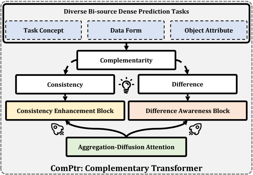
Figure 1: Visual outline of the proposed ComPtr. For diverse bi-source dense prediction tasks, our method is based on the generic concept of complementarity. The consistency enhancement block (Sec. 3.2.3) and difference awareness block (Sec. 3.2.4) are constructed based on the proposed efficient aggregation-diffusion attention (Sec. 3.2.1) from the perspectives of consistency and difference, respectively. Such a design as a whole serves the implementation of the task-generic architecture.

	Input Attributes		Output Attributes
			Object Category Attributes			Task Requirements
Selected Tasks	Single-Modal	Multi-Modal	Class-agnostic	Single-class	Multi-class	Region Seg.	Point Loc.
Remote Sensing Change Detection	✓			✓		✓
RGB-T Crowd Counting		✓		✓			✓
RGB-D/T Salient Object Detection		✓	✓			✓
RGB-D Semantic Segmentation		✓			✓	✓

TABLE I: Attributes of several typical bi-source dense prediction tasks.

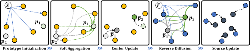
Figure 2: Illustration of our aggregation-diffusion attention (ADA). It implements an efficient alternative to the standard attention to build a global interaction between source feature set $S=\{F^{1},F^{2}\}$ and slot features $F$. In the feature space, the proxy prototype set $P=\{p_{k}\}_{k=1}^{K}$ ($K=2$ in this case) for information interaction is initialized first. Based on the similarity, $S$ is adaptively aggregated into these prototypes and they evolve into $\tilde{P}$. Next, core semantic concepts, which are compressed into the prototypes, are diffused backward to $F$. The thickness of the green and gray arrows represents the relative scale of the weights in the feature reconstruction, where the thicker is larger and vice versa. Best viewed in color.

The complementarity between two inputs can be decomposed into consistency and difference. Based on it, we design a simple yet effective framework ComPtr, as shown in Fig. 3, to address the general bi-source vision modeling. Specifically, we design a complementary transformer, which contains consistency enhancement blocks and difference awareness blocks, i.e., CEM and DAM. The “consistency” tends to highlight the commonality between multi-source data. The CEM blocks are equipped in the encoder to strengthen the object-related representation. While the “difference” depicts the specificity of each stream. We build the DAM-based decoder, which continuously endows the enhanced common representation with scene details from different sources to achieve accurate predictions.

The global dense interaction based on the transformer plays an important role. However, its computational complexity increases quadratically with the length of the input token sequence. This inherent property in the structure of the standard transformer leads to a severe computational burden when dealing with high-resolution features. To alleviate this problem, we design the aggregation-diffusion attention inspired by the K-means algorithm. Specifically, several specific proxy prototypes are inserted into the feature interaction path. It provides an alternative of linear complexity for global information propagation, of which the schematic diagram is shown in Fig. 2.

The main contributions of this paper can be summarized as follows:

1. To the best of our knowledge, it is the first attempt to accomplish the unification of the network architecture for diverse bi-source dense prediction tasks.

2. We build a complementary transformer, ComPtr, by deconstructing the complementarity property of tasks into two aspects: consistency and difference, which effectively enhances global feature interaction and narrows the gaps among multiple tasks.

3. A novel proxy prototype bridging strategy is proposed to construct the aggregation-diffusion attention mechanism, which helps to improve and simplify the global information propagation process.

4. ComPtr achieves state-of-the-art performance on several challenging dataset benchmarks of five representative tasks.

2 Related Work

2.1 Bi-source Dense Prediction

The dense prediction field has a large number of branches, and they have a variety of data forms and task objectives. The bi-source dense prediction tasks can be summarized based on task attributes as listed in Tab. I. From the forms of inputs, there are two categories: single-modal data source and multi-modal data source. According to the attributes of objects, they can be divided into three aspects: class-agnostic, single-class, and multi-class tasks. In addition, their outputs are complete region segmentation (i.e., confidence or binary map) or rough point location (i.e., density estimation). Motivated by these considerations, we select several representative bi-source tasks to explore the general modeling in this work. As shown in Tab. I, they cover all the aforementioned task attributes.

2.1.1 Task-specific Methods

Task-specific methods dominate different tasks, and they use the characteristics and prior information of the task itself as a guide for model design. In remote sensing change detection (RSCD) that aims to explore the dissimilarity of the specific content of bi-temporal images, the exploration of task-inspired difference information has been the main concern of related works. The pioneering work [10] proposes a fully convolutional siamese neural network to perform change detection and this classical architecture is inherited by many follow-up methods. And, single-temporal image segmentation [11, 12] and edge detection [13], which are closely related to RSCD, are introduced as auxiliaries to construct multi-task learning. To enhance the mining process of difference information, recent works [14, 15, 16, 17] begin to incorporate the transformer structure and attention mechanism to model contexts within spatial and temporal domains. In RGB-T crowd counting, the thermal modality plays an important role in poor illumination conditions and is further highlighted because of its sensitivity to the human body. Existing two-stream methods [18, 19] and three-stream [5] aggregate complementary information by designing complex cross-modal interaction structures. Recent work [20] introduces the mutual attention transformer to leverage the cross-modal information. In RGB-D/T salient object detection, the two-stream architecture is the mainstream. [21] uses the dynamic convolution module with depth information to guide feature decoding and achieves more flexible and efficient multi-scale cross-modal feature processing. [22] designs an effective cross-modal fusion and enables the salient boundary via the bilateral fusion strategy. Recently, by introducing the transformer-based dense interaction component, [23, 24, 25, 26] achieve superior results. In RGB-D semantic segmentation, the geometric prior of depth information is fully depicted and utilized. [27, 28] use the depth modality to help the convolution layer adjust the receptive field and adapt to geometric transformations. [29] designs a depth-specific convolution layer and pays more attention to shape information by re-weighting the shape component and the base component of the depth feature. And [30] proposes a pixel differential convolution attention module to capture long-range dependency for RGB data and local geometric consistency for depth data. [31] builds a k-nearest neighbor graph based on position and depth information. All the above-mentioned schemes, without exception, focus on task-specific information mining. They make full use of task-prior knowledge to obtain more inductive bias.

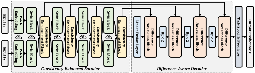
Figure 3: Overview of the proposed ComPtr framework. It follows the two-branch encoder-decoder architecture which is commonly used in diverse bi-source dense prediction tasks. indicates that the corresponding module shares parameters.

2.1.2 Task-generic Methods

The task-generic design can improve the efficiency of data utilization and take a solid step towards a more intelligent algorithm by integrating knowledge of various tasks. The existing task-generic models can be roughly classified into three categories: the large-scale pre-training task-independent architecture [32, 33], the multi-task joint learning framework [34] and the transferable general single-task architecture [25, 26]. This paper belongs to the last one. Although several recent approaches [25, 26] have attempted to explore the cross-task unified architecture, they only focus on a single field (SOD). There is a large room in the extension of task concepts, data forms, and object attributes, which is exactly what we focus on in this work.

2.2 Transformer-based Methods

Long-range context information is crucial for accurate scene understanding, which has been verified in many existing works [35, 36, 37]. Due to the built-in long-range dependence modeling without induction bias, the non-local operation like the non-local block [38] and self-attention in transformer [1, 39, 2], has become an important component for capturing the global context cues. Recently, several transformer-based approaches have been proposed for bi-source dense prediction tasks. Most of those methods [17, 24, 25, 26, 40, 20] follow the design pattern of using independent encoders for different sources. They apply vision transformers to construct hierarchical representations and ignore the complementarity characterization in the encoder stage. Moreover, their interaction units based on standard attention also limit the scalability of their structure [17, 24, 20, 26]. Different from them, we use the proxy prototype mechanism inspired by the clustering algorithm to transform the global interaction of complementary information into two sequential steps of aggregation and diffusion. This design effectively improves the scalability of the proposed architecture for different tasks and plays a positive role in realizing a general model for diverse bi-source dense prediction tasks.

3 Methodology

In this section, we first present the overall structure of the proposed ComPtr and then introduce the details of the different components in sequence.

3.1 Overall Architecture

Following the two-branch encoder-decoder architecture which is commonly used in diverse bi-source dense prediction tasks [10, 23, 26, 22, 41], we design a complementary transformer (ComPtr) framework. Considering that complementarity plays an important role in the bi-source dense prediction task, this concept is decomposed into two parts, i.e., consistency and difference, in the proposed model. And they lead the improvement and design of the encoder and decoder respectively. As shown in Fig. 3, ComPtr is composed of these basic components: a parameter-shared feature extractor, several consistency enhancement and difference awareness blocks, and a light task-specific predictor.

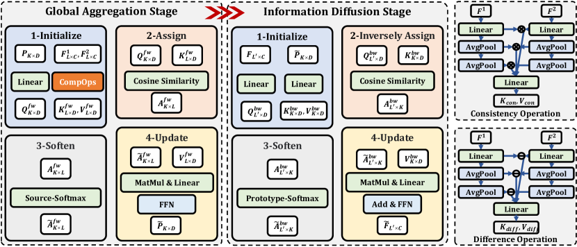
Figure 4: Details of the proposed aggregation-diffusion attention mechanism (ADA) which construct the interaction between the source features $F^{1},F^{2}\in\mathbb{R}^{L\times C}$ and the slot feature $F\in\mathbb{R}^{L^{\prime}\times C}$ mediated by the learnable proxy prototype $P\in\mathbb{R}^{K\times D}$. It contains two stages executed sequentially: a forward global aggregation stage (“fw”) and a backward information diffusion stage (“bw”). “CompOps” represents the complementarity operations as shown on the right: the multi-granularity consistency operation and the hierarchical difference operation. and generate the element-wise product and the absolute difference of the two inputs. Some normalization and activation layers are dropped here for notational brevity.

3.1.1 Consistency-Enhanced Encoder

We directly choose the relatively frequently-used Swin Transformer [2] to realize the function of feature extraction which consists of several non-overlap patch embedding layers and swin transformer blocks built on the shifted window based self-attention. The siamese design with shared parameters is also introduced here like [10] to simplify the model design and reduce the number of parameters. Besides, the proposed consistency enhancement component is inserted into the basic feature extractor to build the consistency enhanced encoder as depicted on the left of Fig. 3, which allows each stream to be strengthened with specific important cues while maintaining its own specificity.

3.1.2 Difference-Aware Decoder

In the decoder, the deepest two-stream features are merged by a simple linear fusion layer only containing normalization and linear layers. The result is delivered to a cascaded difference awareness block and intersects with the shallow encoder features, which absorbs the difference information at the specific scale between the two streams. Together with the subsequent stacked interpolation operations, difference awareness blocks, and task-specific predictor, they form the difference-aware decoder as shown on the right of Fig 3. On the basis of features enhanced by consistency-related patterns, the model continuously absorbs inter-source specificity information at different scales to achieve accurate task-specific decoding.

3.1.3 Light Task-specific predictor

To adapt to different types of tasks, we introduce several lightweight task-specific predictors by simply combining interpolation, normalization, activation, and linear layers.

3.2 Complementary Transformer

The consistency enhancement and difference awareness blocks are all based on a novel and efficient global aggregation-diffusion attention mechanism (ADA), but there are obvious differences in the details.

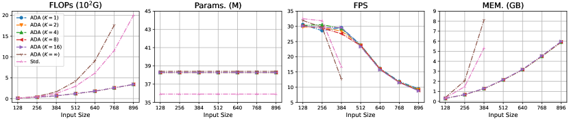
Figure 5: Comparison of the proposed ADA with the standard attention form “Std.” in terms of the amount of computation (“GFLOPs”), the number of parameters (“Params.”), the inference speed (“FPS”), and the peak memory usage (“MEM.”). And these results are collected in the inference mode, focusing on the inference efficiency of the model. It is worth noting that the FPS and MEM. of “ADA (K=$\infty$)” and “Std.” cannot be evaluated with input sizes larger than $384\times 384$ due to their huge memory requirements. More details can be found in Sec. 3.2.2 and Sec. 4.7.1.

3.2.1 Aggregation-Diffusion Attention

In order to build a more effective dense interaction between the features from the two sources to promote the mining and dissemination of global complementary information, we introduce the transformer architecture. Although it has powerful information modeling and interaction capabilities, its global dense interaction form also causes a non-negligible quadratic computational complexity with respect to the length of the input sequence. Inspired by the K-means clustering algorithm, we introduce the proxy prototype as the mediator for global information propagation. And the straight-through dense interaction of the standard attention is decoupled and reconstructed into two different stages: the forward global aggregation and the backward information diffusion as depicted in Fig. 4.

In the aggregation stage, the attribute-specific key and value $K^{fw},V^{fw}\in\mathbb{R}^{L\times D}(L=H\times W)$ are generated from two-stream source feature set $S=\{F^{i}\}^{2}_{i=1},F^{i}\in\mathbb{R}^{L\times C}$ by the complementarity operation $\mathtt{CompOps}$. And $K$ learnable $D$-dimensional proxy prototype vectors $P=\{p_{i}\}_{i=1}^{K}$ are also transformed to the same channel dimension $D$ by a linear projection weight $W^{fw}_{Q}$. The above process can be formulated as:

$$K^{fw},V^{fw}=\mathtt{CompOps}(F^{1},F^{2}),$$ (1)

$$Q^{fw}=PW^{fw}_{Q},\quad W^{fw}_{Q}\in\mathbb{R}^{D\times D}.$$ (2)

Inspired by the similarity-based information aggregation in K-means, the pair-wise $\mathtt{cosine}$ similarity between the source embedding and the proxy prototype $P$ is served as the basis for assigning the global information in the aggregation process, which can be expressed mathematically as:

$$\begin{gathered}A^{fw}=\mathtt{cosine}(Q^{fw},K^{fw}).\end{gathered}$$ (3)

The next steps are similar to the centralization process in K-means. Different from the hard sample selection mechanism ($\mathtt{argmax}$) in K-means, $\mathtt{softmax}$ is chosen to soften the process and ensure the differentiability of the calculation. So we can get the normalized similarity as follows:

$$\begin{gathered}\tilde{A}^{fw}=\mathtt{softmax}(A^{fw}).\end{gathered}$$ (4)

And a similarity-based transformation is introduced to integrate the more important cues from the transformed input $V^{fw}$ into the proxy prototype $P$. The updated proxy prototype $\tilde{P}\in\mathbb{R}^{K\times D}$ can be obtained as follows:

$$\begin{gathered}\tilde{P}=\mathtt{FFN}((\tilde{A}^{fw}V^{fw})W^{fw}_{O}),\quad W^{fw}_{O}\in\mathbb{R}^{D\times D},\end{gathered}$$ (5)

where $\mathtt{FFN}$ is a forward feed network containing normalization, linear and activation layers.

And in the diffusion stage, the proxy prototype $\tilde{P}$, acting as a mediator, diffuse these global semantics back into the original image space, and this procedure can also be considered as reversed K-means. At this time, the image feature $F\in\mathbb{R}^{L^{\prime}\times C}$, i.e., the diffusion slot, can supplement the complement information from the prototype $\tilde{P}$ based on the similarity relationship. Specifically, after the specific linear transformation by $W^{bw}_{Q}$ and $W^{bw}_{K}$, both $F$ and $\tilde{P}$ are involved in the calculation of the correlation, which can generate the similarity $A^{bw}$ after the $\mathtt{cosine}$ operation as following:

$$\begin{gathered}Q^{bw}=FW^{bw}_{Q},\quad W^{bw}_{Q}\in\mathbb{R}^{C\times D},\\ K^{bw}=\tilde{P}W^{bw}_{K},\quad W^{bw}_{K}\in\mathbb{R}^{D\times D},\\ A^{bw}=\mathtt{cosine}(Q^{bw},K^{bw}).\end{gathered}$$ (6)

The $\mathtt{softmax}$ function is imposed on $A^{bw}$ to normalize the importance of different prototypes and modulate the subsequent feature reconstruction based on $\tilde{P}$. And it can be mathematically expressed as follows:

$$\begin{gathered}\tilde{A}^{bw}=\mathtt{softmax}(A^{bw}),\\ V^{bw}=\tilde{P}W^{bw}_{V},\quad W^{bw}_{V}\in\mathbb{R}^{D\times D},\\ Z^{bw}=\tilde{A}^{bw}V^{bw}W^{bw}_{O},\quad W^{bw}_{O}\in\mathbb{R}^{D\times C}.\end{gathered}$$ (7)

And the residual connection and learnable vector $\gamma\in\mathbb{R}^{D}$ are introduced to balance the attention output $Z^{bw}$ and the input slot feature $F$, where $\gamma$ is initialized with the zero value to ensure the original feature distribution in the early stage of training as [39]:

$$\begin{gathered}\tilde{F}=F+\mathtt{FFN}(F+\gamma\odot Z^{bw}),\end{gathered}$$ (8)

where $\odot$ denotes the element-wise multiplication. The successive aggregation and diffusion phases realize the global interaction based on the proxy prototype.

3.2.2 Comparison with standard attention

For a $D$-dimensional image token sequence of length $L=H\times W$, the computational complexity and the memory footprint of the standard attention are approximately $O(L^{2}\times D)$ and $O(L^{2})$. Compared with the standard attention, the proposed proxy prototype bridging strategy effectively reduces the computation and memory of dense global interaction to linear complexity ($O(L\times K\times D+L\times K\times D)$ and $O(L\times K+L\times K)$), where $K$ is the number of proxy prototypes. Considering that $K$ is a small constant, i.e. $K\ll L$, the proposed aggregation-diffusion attention is more efficient than the standard form. In order to visualize the difference in inference efficiency, we show the comparison of the proposed ADA with the standard attention for different resolutions of the input in Fig. 5, and more details and analyses can be found in Sec. 4.7.1.

3.2.3 Consistency Enhancement Block (CEB)

By introducing the consistency operation into the proposed aggregation-diffusion attention, we design the CEB to strengthen the common visual cues and help the model obtain a more powerful data representation. And the consistency-specialized key and value embeddings $K_{con}$ and $V_{con}$ can be obtained by the multi-granularity element-wise multiplication of the two image source feature inputs $F^{1}$ and $F^{2}$ from different streams as shown on the top right-hand corner of Fig. 4. They are used as $K^{fw}$ and $V^{fw}$ in Equ. 1. Specifically, the consistency operation is composed of several normalization, linear, and pooling layers. With the aid of two parameter-free average pooling layers, we can obtain products $\{F^{i}_{con}\}_{i=1}^{3}$ from three different scales. After concatenating and transformed along the channel, a complete multi-scale consistency representation is generated from the inputs. It is split into $K_{con}$ and $V_{con}$ along the channel which participate in the update process of the proxy prototype $P$. In the diffusion stage, the slot feature $F$ with $L^{\prime}=2HW$ is the concatenation of the image features $F^{1}$ and $F^{2}$ along the flatten spatial dimension. It is reconstructed independently to $\tilde{F}$ based on the updated proxy prototype $\tilde{P}$. And these enhanced features $\tilde{F}^{1}$ and $\tilde{F}^{2}$ stored in the slot $\tilde{F}$ replace original $F^{1}$ and $F^{2}$ as the input of the next swin transformer block.

3.2.4 Difference Awareness Block (DAB)

This block differs from the CEB in two aspects, one is the generation of embeddings $K_{diff}$ and $V_{diff}$ based on the source features, and the other is the global diffusion way of the assigned information. As shown on the bottom right-hand corner of Fig. 4, a hierarchical difference operation containing normalization, linear and pooling layers are embedded here to obtain the multi-granularity absolute difference representation $K_{diff}$ and $V_{diff}$, which are used as $K^{fw}$ and $V^{fw}$ in Equ. 1. Besides, the slot feature $F$ with $L^{\prime}=HW$ in the diffusion stage is a compact hybrid representation, which comes from the initial fusion of the encoder features $F^{1}$ and $F^{2}$, and the deeper DAB feature $\tilde{F}^{\prime}$ through several stacked linear layers. The output slot feature $\tilde{F}$ of the block is fed into the subsequent module and involved in the decoding process of the high-resolution prediction.

3.2.5 Loss Function

For a fair comparison with existing approaches, we use the commonly used loss functions for each task. In remote sensing change detection, RGB-D/T salient object detection, and RGB-D semantic segmentation tasks, the binary or multi-class cross-entropy loss is used to supervise the training of the model. In RGB-T crowd counting, we follow the loss form of [40] containing the distribution matching loss proposed in [42] for density map estimation and an L1 loss for counting regression.

4 Experiments

		LEVIR-CD [3]					SYSU-CD [4]
Methods	Backbone	Pre. $\uparrow$	Rec. $\uparrow$	F1 $\uparrow$	IOU $\uparrow$	OA $\uparrow$	Pre. $\uparrow$	Rec. $\uparrow$	F1 $\uparrow$	IOU $\uparrow$	OA $\uparrow$
FC-EF18 [10]	UNet	.8556	.7876	.8202	.6952	.9824	.7228	.7285	.7257	.5694	.8701
FC-Siam-Di18 [10]	UNet	.9153	.7824	.8436	.7295	.9852	.8494	.5145	.6408	.4715	.8640
FC-Siam-Conc18 [10]	UNet	.8417	.7949	.8177	.6916	.9819	.8303	.7162	.7689	.6245	.8935
FresUNet19 [11]	UNet	.8986	.8641	.8905	.8026	.9892	.7856	.7496	.7638	.6185	.8912
IFNet20 [14]	VGG-16	.9439	.8242	.8801	.7858	.9886	.7959	.7358	.7653	.6191	.8917
DTCDSCN21 [12]	SE-ResNet-32	.8925	.8568	.8743	.7767	.9875	.8319	.7725	.8011	.6682	.9096
SNUNet22 [43]	NestedUNet	.8918	.8717	.8816	.7883	.9882	.8349	.7637	.7977	.6635	.9087
BIT22 [15]	ResNet-18	.8924	.8937	.8931	.8068	.9892	.7873	.7568	.7717	.6283	.8944
EGRCNN22 [13]	UNet	.9283	.8646	.8959	.8112	.9892	.8436	.7841	.8164	.6902	.9164
MSPSNet22 [44]	MSSNN [44]	.9138	.8708	.8918	.8136	.9903	.7847	.7491	.7739	.6313	.8943
ICIFNet22 [16]	ResNet-18+PVT-V2-B1	.9132	.8864	.8996	.8175	.9899	.8337	.7851	.8074	.6812	.9124
DMINet23 [17]	ResNet-18	.9252	.8995	.9071	.8299	.9907	.8503	.7986	.8208	.6960	.9167
ComPtr-T23	Swin-T	.9336	.9091	.9212	.8539	.9921	.8638	.7896	.8250	.7021	.9210
ComPtr-B23	Swin-B	.9349	.9078	.9211	.8538	.9921	.8726	.7903	.8294	.7086	.9233

TABLE II: Comparison on the testing datasets of LEVIR-CD and SYSU-CD for RSCD. Colors red, green and blue in all tables represent the first, second and third ranked results.

Methods	Bsckbone	GAME0 $\downarrow$	GAME1 $\downarrow$	GAME2 $\downarrow$	GAME3 $\downarrow$	RMSE $\downarrow$
CSRNet18 [45]	VGG-16	20.40	23.58	28.03	35.51	35.26
BL19 [46]	VGG-19	18.70	22.55	26.83	34.62	32.67
DM-Count20 [42]	VGG-19	16.54	20.73	25.23	32.23	27.22
P2PNet21 [47]	VGG-16	16.24	19.42	23.48	30.27	29.94
MARUNet21 [48]	VGG-16	17.39	20.54	23.69	27.36	30.84
MAN22 [49]	VGG-19	17.16	21.78	28.74	41.59	33.84
CMCRL21 [18]	VGG-16	15.61	19.95	24.69	32.89	28.18
TAFNet22 [5]	VGG-16	12.38	16.98	21.86	30.19	22.45
MAT22 [20]	VGG-16	12.35	16.29	20.81	29.09	22.53
DEFNet22 [19]	VGG-16	11.90	16.08	20.19	27.27	21.09
MMCC22 [40]	PVT-V2-B3	10.90	14.81	19.02	26.14	18.79
ComPtr-T23	Swin-T	10.52	14.51	18.48	24.28	18.48
ComPtr-B23	Swin-B	11.82	15.84	20.17	26.41	20.75

TABLE III: Comparison on RGBT-CC [5] testing dataset. The top six single-modal methods are retrained by [40] and the others are bi-modal methods.

		DUTLF-Depth [50]					NJUD [51]					NLPR [52]					SIP [53]					STEREO1000 [54]
Methods	Backbone	$S_{m}$ $\uparrow$	$F^{\omega}_{\beta}$ $\uparrow$	MAE $\downarrow$	$E_{m}$ $\uparrow$	$F_{\beta}$ $\uparrow$	$S_{m}$ $\uparrow$	$F^{\omega}_{\beta}$ $\uparrow$	MAE $\downarrow$	$E_{m}$ $\uparrow$	$F_{\beta}$ $\uparrow$	$S_{m}$ $\uparrow$	$F^{\omega}_{\beta}$ $\uparrow$	MAE $\downarrow$	$E_{m}$ $\uparrow$	$F_{\beta}$ $\uparrow$	$S_{m}$ $\uparrow$	$F^{\omega}_{\beta}$ $\uparrow$	MAE $\downarrow$	$E_{m}$ $\uparrow$	$F_{\beta}$ $\uparrow$	$S_{m}$ $\uparrow$	$F^{\omega}_{\beta}$ $\uparrow$	MAE $\downarrow$	$E_{m}$ $\uparrow$	$F_{\beta}$ $\uparrow$
JLDCF20 [55]	ResNet-101	.9052	.8633	.0429	.9426	.9112	.9022	.8691	.0413	.9437	.9042	.9250	.8820	.0216	.9627	.9176	.8804	.8438	.0491	.9247	.8890	.9026	.8570	.0403	.9468	.9039
HDFNet20 [21]	ResNet-50	.9072	.8640	.0413	.9473	.9176	.9079	.8772	.0381	.9442	.9107	.9232	.8822	.0228	.9629	.9171	.8859	.8477	.0472	.9297	.8938	.8997	.8526	.0413	.9434	.8996
D3Net20 [53]	VGG-19	.7753	.6680	.0967	.8330	.7417	.9005	.8541	.0463	.9385	.9000	.9117	.8486	.0296	.9530	.8969	.8603	.7989	.0631	.9086	.8611	.8986	.8378	.0458	.9383	.8912
RD3D21 [56]	I3DResNet-50	.9313	.9074	.0311	.9597	.9387	.9156	.8855	.0365	.9471	.9139	.9296	.8887	.0221	.9649	.9190	.8853	.8449	.0484	.9243	.8890	.9113	.8706	.0374	.9466	.9061
TriTransNet21 [23]	ResNet-50+ViT-B	.9326	.9263	.0249	.9657	.9463	.9196	.9059	.0303	.9550	.9263	.9284	.9018	.0204	.9662	.9238	.8861	.8642	.0434	.9303	.8988	.9078	.8816	.0333	.9532	.9114
DCF21 [57]	ResNet-50	.9240	.9094	.0301	.9571	.9319	.9037	.8765	.0387	.9431	.9052	.9220	.8841	.0235	.9574	.9099	.8735	.8397	.0519	.9218	.8859	.9057	.8719	.0370	.9477	.9044
DSA2F21 [58]	VGG-19	.9218	.9073	.0309	.9581	.9326	.9043	.8819	.0394	.9387	.9074	.9188	.8800	.0242	.9523	.9059	.8620	.8277	.0574	.9121	.8754	.8978	.8679	.0387	.9420	.8996
CMINet${}^{\star}_{21}$ [59]	ResNet-50	.8968	.8666	.0461	.9258	.8909	.9286	.9095	.0286	.9574	.9336	.9317	.9001	.0205	.9624	.9223	.8985	.8717	.0404	.9389	.9099	.9183	.8855	.0323	.9512	.9164
SPNet21 [60]	Res2Net-50	.8041	.7346	.0853	.9098	.8489	.9245	.9061	.0285	.9572	.9280	.9273	.8960	.0208	.9616	.9185	.8937	.8675	.0430	.9328	.9036	.9068	.8731	.0369	.9487	.9063
VST21 [24]	T2T-ViT-t14	.9425	.9205	.0250	.9708	.9490	.9224	.8882	.0343	.9510	.9195	.9314	.8866	.0233	.9623	.9201	.9036	.8725	.0396	.9439	.9150	.9128	.8656	.0376	.9506	.9067
HAINet21 [61]	VGG-16	.9095	.8832	.0381	.9442	.9198	.9093	.8786	.0384	.9405	.9095	.9210	.8807	.0250	.9538	.9079	.8861	.8542	.0484	.9271	.9026	.9093	.8714	.0380	.9471	.9093
CCAFNet21 [62]	VGG-16	.9040	.8781	.0377	.9431	.9132	.9101	.8765	.0374	.9440	.9099	.9221	.8748	.0267	.9567	.9087	.8769	.8293	.0544	.9165	.8804	.8917	.8440	.0446	.9342	.8865
DCMF22 [63]	VGG-16	.9279	.8885	.0350	.9582	.9319	.9126	.8669	.0426	.9479	.9154	.9220	.8562	.0287	.9541	.9056	.8700	.8084	.0618	.9110	.8719	.9097	.8487	.0426	.9464	.9063
SwinNet22 [25]	Swin-B	.9336	.9128	.0290	.9625	.9404	.9347	.9127	.0271	.9633	.9382	.9413	.9084	.0179	.9736	.9361	.9113	.8900	.0352	.9498	.9270	.9193	.8821	.0328	.9560	.9178
CAVER23 [26]	ResNet-101D	.9374	.9258	.0259	.9675	.9463	.9255	.9060	.0289	.9588	.9283	.9341	.9042	.0208	.9700	.9290	.9039	.8787	.0370	.9447	.9151	.9174	.8878	.0319	.9552	.9161
ComPtr-T23	Swin-T	.9437	.9217	.0250	.9699	.9506	.9289	.8948	.0327	.9584	.9299	.9356	.8866	.0214	.9668	.9240	.9134	.8796	.0361	.9499	.9211	.9199	.8745	.0348	.9547	.9155
ComPtr-B23	Swin-B	.9587	.9514	.0169	.9819	.9680	.9396	.9195	.0249	.9664	.9446	.9429	.9073	.0194	.9711	.9357	.9153	.8948	.0337	.9504	.9307	.9329	.9029	.0279	.9623	.9324

TABLE IV: Experiments on five RGB-D SOD benchmarks. “$\star$”: Using the multi-scale training strategy.

		VT821 [64]					VT1000 [65]					VT5000 [41]
Methods	Backbone	$S_{m}$ $\uparrow$	$F^{\omega}_{\beta}$ $\uparrow$	MAE $\downarrow$	$E_{m}$ $\uparrow$	$F_{\beta}$ $\uparrow$	$S_{m}$ $\uparrow$	$F^{\omega}_{\beta}$ $\uparrow$	MAE $\downarrow$	$E_{m}$ $\uparrow$	$F_{\beta}$ $\uparrow$	$S_{m}$ $\uparrow$	$F^{\omega}_{\beta}$ $\uparrow$	MAE $\downarrow$	$E_{m}$ $\uparrow$	$F_{\beta}$ $\uparrow$
MTMR18 [64]	—	.5927	.2639	.2595	.8108	.6464	.7057	.4854	.1194	.8359	.7154	.6801	.3968	.1143	.7923	.6133
M3S-NIR19 [66]	—	.7231	.4072	.1397	.8371	.7378	.7258	.4628	.1454	.8279	.7353	.6521	.3271	.1680	.7599	.5957
ADF20 [41]	—	.8102	.6265	.0765	.8389	.7522	.9095	.8043	.0339	.9505	.9081	.8635	.7218	.0482	.9111	.8368
SDGL20 [65]	VGG-19	.7654	.5828	.0849	.8395	.7347	.7867	.6524	.0896	.8585	.7700	.7504	.5585	.0886	.8292	.6949
CSRNet21 [67]	ESPNetv2 [68]	.8847	.8212	.0376	.9226	.8579	.9183	.8782	.0242	.9526	.9083	.8675	.7964	.0417	.9138	.8370
ECFFNet21 [22]	ResNet-34	.8771	.7993	.0347	.9103	.8352	.9238	.8835	.0217	.9593	.9171	.8745	.7998	.0379	.9212	.8461
MIDD21 [69]	VGG-16	.8710	.7596	.0445	.9183	.8508	.9154	.8558	.0271	.9567	.9128	.8674	.7629	.0432	.9201	.8491
CGFNet21 [70]	VGG-16	.8805	.8287	.0378	.9204	.8658	.9232	.8999	.0231	.9594	.9235	.8830	.8311	.0353	.9265	.8690
SwinNet22 [25]	Swin-B	.9037	.8183	.0298	.9387	.8809	.9381	.8936	.0179	.9743	.9409	.9117	.8461	.0258	.9538	.9018
CAVER23 [26]	ResNet-101D	.8978	.8462	.0264	.9340	.8767	.9376	.9124	.0164	.9728	.9393	.8994	.8489	.0284	.9439	.8818
ComPtr-T23	Swin-T	.9034	.8279	.0300	.9369	.8826	.9395	.8936	.0202	.9731	.9409	.9053	.8259	.0313	.9467	.8861
ComPtr-B23	Swin-B	.9151	.8553	.0247	.9447	.8943	.9456	.9126	.0172	.9772	.9462	.9197	.8604	.0244	.9597	.9064

TABLE V: Comparison on three RGB-T SOD benchmarks. “—”: Traditional methods based on hand-crafted features.

Methods	Backbone	Pixel Acc. $\uparrow$	Mean Acc. $\uparrow$	Mean IOU $\uparrow$
3DGNN17 [31]	VGG-16	—	.557	.431
LSD-GF17 [71]	VGG-16	.719	.607	.459
RDF17 [72]	ResNet-152	.760	.628	.501
MMAF-Net19 [73]	ResNet-152	.722	.592	.448
ACNet19 [74]	ResNet-50	—	—	.483
SA-Gate20 [75]	ResNet-101	.779	—	.524
Malleable 2.5D20 [76]	ResNet-101	.769	—	.509
SGNet21 [28]	ResNet-101	.768	.633	.511
NANet21 [77]	ResNet-101	.779	—	.523
ShapeConv21 [29]	ResNeXt-101	.764	.635	.513
InverseForm21 [78]	ResNet-101	.781	—	.531
DCANet22 [30]	ResNet-101	.782	—	.533
PDCNet23 [79]	ResNet-101	.784	—	.535
ComPtr-T23	Swin-T	.758	.615	.492
ComPtr-B23	Swin-B	.795	.686	.555

TABLE VI: Comparison on NYU-Depth V2 (40 classes) [9] benchmark for RGB-D SS. “—”: Not available.

To verify the generality, transferability and effectiveness of the proposed architecture, we select four types of important bi-source tasks with large diversity: remote sensing change detection (RSCD), RGB-T crowd counting (RGB-T CC), RGB-D/T salient object detection (RGB-D/T SOD), and RGB-D semantic segmentation (RGB-D SS). Specific experimental details are presented in the following sections.

4.1 Basic Training Settings

In all experiments, we use Swin Transformer [2] pre-trained from ImageNet [80] as the initial parameters of the feature extractor for all tasks, while other parts are randomly initialized by PyTorch. The three-channel image is normalized, while the single-channel one only replicates three times along the channel after dividing by 255. The AdamW [81] optimizer is consistently used due to its suitability for the transformer architecture. The settings of other hyper-parameters for different tasks mostly follow those of the existing algorithms [17, 40, 26, 25, 60, 22, 75] to achieve a more fair comparison, and more task-specific details are shown in the corresponding sections.

4.2 Remote Sensing Change Detection (RSCD)

Datasets. Two commonly used large-scale data benchmarks are used to evaluate performance, namely LEarning, VIsion, and Remote sensing (LEVIR-CD) [3] and Sun Yat-Sen University Dataset (SYSU-CD) [4]. LEVIR-CD is a large-scale and very-high-resolution (VHR) RSCD dataset collected via Google Earth API. It contains 637 pairs of real bi-temporal RGB image patches with a time span of 5-14 years, a size of $1024\times 1024$, a spatial resolution of 0.5 m/pixel and a total of 31333 individual change buildings. The dataset is split into training/validation/testing sets in a 7:1:2 ratio and each sample is cropped to 16 small patches with a size of $256\times 256$ for decreasing the computational cost. The recently proposed SYSU-CD is another important and challenging benchmark containing 20000 pairs of 0.5 m/pixel aerial images taken between the years 2007 and 2014 in Hong Kong. These images with a shape of $256\times 256$ are divided into training/validation/testing sets with 12000/4000/4000 image pairs. The model is trained, validated, and tested independently on each dataset. Following the existing methods [17, 16, 15], image patches with a shape of $256\times 256$ and a batch size of 16 are augmented using random scaling, affine transformation, flipping, and color jitter during training. For the experiments on the LEVIR-CD dataset, we train the model for 200 epochs and use the cosine scheduler with an initial learning rate of 0.0002 and a weight decay of 0.0005. On SYSU-CD, to alleviate the over-fitting problem, we introduced the one-cycle scheduler [82] with a large learning rate of 0.001 and a weight decay of 0.0005, which can play a role of regularization, and the number of training epochs is reduced to a quarter of the one on LEVIR-CD.

Metrics. For the comparison between the change prediction map and the ground truth, we introduce five common binary image similarity metrics, including precision (Pre.), recall (Rec.), F1-score (F1), intersection over union (IOU) and overall accuracy (OA). And they can be mathematically formalized as follows:

$$\mathrm{Pre.}=\frac{TP}{TP+FP},$$ (9)

$$\mathrm{Rec.}=\frac{TP}{TP+FN},$$ (10)

$$\mathrm{F1}=\frac{2TP}{2TP+FN+FP},$$ (11)

$$\mathrm{IOU}=\frac{TP}{TP+FP+FN},$$ (12)

$$\mathrm{OA}=\frac{TP+TN}{TP+TN+FP+FN},$$ (13)

where TP, TN, FP, and FN are the number of true positive, true negative, false positive, and false negative samples in the binary prediction, respectively. Since F1 and IOU implicitly consider both Pre. and Rec., they can reflect the performance of the model more generally.

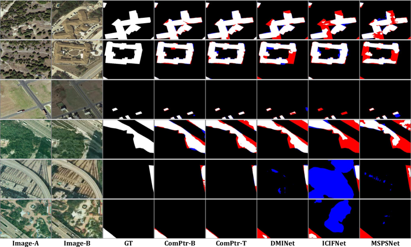
Figure 6: Visual comparison on LEVIR-CD [3] in the top three rows and SYSU-CD [4] in the bottom three rows for remote sensing change detection. Red and blue colors in the binary prediction indicate false negative and false positive regions.

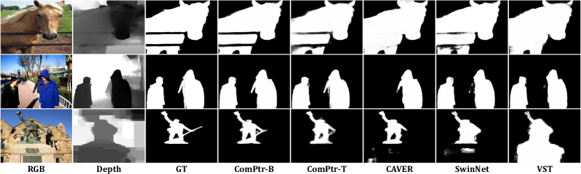
Figure 7: Visual comparison for RGB-D salient object detection.

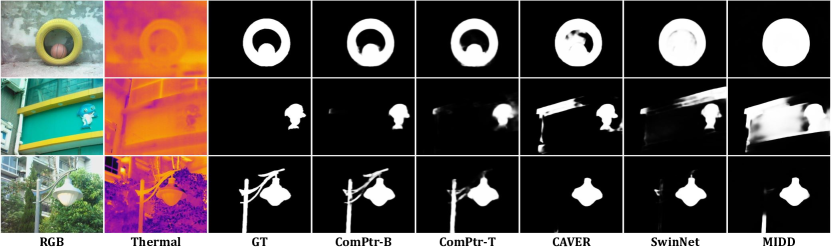
Figure 8: Visual comparison for RGB-T salient object detection.

4.3 RGB-T Crowd Counting (RGB-T CC)

Datasets. In the pioneering work [5], a new large-scale point-annotated dataset benchmark RGBT-CC is carefully collected and manually aligned by an optical-thermal camera and contains 2030 RGB-T pairs with 138389 point-annotated people. All samples have a standard resolution of $640\times 480$. 1013 pairs are captured in the light and 1017 pairs are taken from some dark scenes. The number of the training, validation and testing sets is 1030, 200 and 800, respectively. The model is trained, validated, and tested independently on these datasets like the existing methods [17, 40]. All settings are aligned with the recent best practice [40], where the batch size, learning rate, weight decay, epoch, and crop size are set to 16, 0.00001, 0.0001, 500, $224\times 224$. And no data augmentation other than random cropping is used for this task.

Metrics. For RGB-T CC, five regression metrics are utilized to evaluate the regression error, which include four levels of grid average mean absolute error [83] (GAME_i, $i\in\{0,1,2,3\}$) and root mean square error (RMSE). To calculate GAME, the density prediction and the ground truth are grided into $4^{i}$ ($i\in\{0,1,2,3\}$) parts.

$$\mathrm{GAME}_{i}=\frac{1}{N}\sum^{N}_{n=1}\sum^{4^{i}}_{j=1}|P^{j}_{n}-G^{j}_{n}|,$$ (14)

where $P^{j}_{n}$ and $G^{j}_{n}$ are the count prediction and ground truth in $j^{th}$ part of $n^{th}$ test image pairs. RMSE is mathematically defined as:

$$\mathrm{RMSE}=\sqrt{\frac{1}{N}\sum^{N}_{n=1}(P_{n}-G_{n})^{2}},$$ (15)

where $P_{n}$ and $G_{n}$ are the predicted count and ground truth of $n^{th}$ test image pairs.

4.4 RGB-D/T Salient Object Detection (RGB-D SOD)

Datasets. For RGB-D SOD, we introduce five datasets NJUD [51], NLPR [52], STEREO1000 [54], SIP [53], and DUTLF-Depth [50]. NJUD consists of 1985 image pairs involving a lot of complex scenarios. In NLPR, 1000 RGB-D image pairs are collected from diverse indoor and outdoor scenes. STEREO1000 is composed of 1000 RGB-D image pairs from Flickr, NVIDIA 3D Vision Live and Stereoscopic Image Gallery. SIP containing 929 pairs of high-resolution person images is captured in an outdoor scene. Complex lighting conditions, extreme contrast, and variable pose of people all increase the difficulty of this dataset. DUTLF-Depth is larger in scale and its content is also much richer. It collects 800 pairs of indoor and 400 pairs of outdoor RGB-D images, which contain a large number of challenging objects and scenes. Continuing the setup of existing methods [26, 61, 23], we directly use the same 2985 images from NJUD, NLPR, and DUTLF-Depth to train the model and evaluate it on the remaining data. And for RGB-T SOD, VT821 [64], VT1000 [65], and VT5000 [41] are introduced as the benchmark. VT821 is a pioneering RGB-T SOD datasets, which includes 821 RGB-Thermal-GT image pairs. VT1000 containing 1000 pairs of images, increases the scale of the RGB-T SOD dataset and covers more than 400 kinds of objects in more than 10 types of scenes with diverse lighting conditions. VT5000 contains 5000 pairs of densely annotated RGB-T images, which greatly enriches the diversity and complexity of the task. And this dataset is divided into training and testing sets, each of which has 2500 image pairs. Except for the training set containing 2500 image pairs of VT5000 for training, the rest of the data are used for testing as [25, 26]. On RGB-D/T SOD, the batch size, learning rate, and input shape are consistently set to 16, 0.0002, and $256\times 256$ for ComPtr-T as [26] ($384\times 384$ for ComPtr-B as [25]). Following [60, 22, 25, 26], random affine transformation, flipping, color jittering are introduced as the data augmentation and our models are trained for 100 epochs in RGB-T SOD and 200 epochs in RGB-D SOD with the cosine scheduler.

Metrics. For RGB-D SOD, all methods are evaluated based on five gray-scale image metrics, S-measure [84] ($S_{m}$), maximum F-measure [85] ($F_{\beta}$), maximum E-measure [86] ($E_{m}$), weighted F-measure [87] ($F^{\omega}_{\beta}$), and MAE. $S_{m}$ focuses on region-aware and object-aware structural similarities $S_{r}$ and $S_{o}$, between the saliency map and the ground truth. It can be expressed as: $S_{m}=\alpha S_{o}+(1-\alpha)S_{r}$, where $\alpha$ is set to $0.5$. $F_{\beta}$ is a region-based similarity metric based on precision and recall. The mathematical form is: $F_{\beta}=\frac{(1+\beta^{2})precision\times recall}{\beta^{2}precision+recall}$, where $\beta^{2}$ is generally set to $0.3$ to emphasize more on the precision. $E_{m}$ is composed of local pixel values and the image-level mean value to jointly evaluate the similarity between the prediction and the ground truth. $F^{\omega}_{\beta}$ improves the existing metric $F_{\beta}$ by using a weighted precision for measuring exactness and a weighted recall for measuring completeness. MAE indicates the average absolute pixel error. It is worth noting that the evaluation of the SOD task is based on the gray-scale prediction map. The value of the predicted result indicates the probability of the corresponding position belonging to the salient object region. So, both the calculation process and the formula details of $F_{\beta}$ and $F1$ mentioned in Sec. 4.2 are different, which serves the specific task requirements.

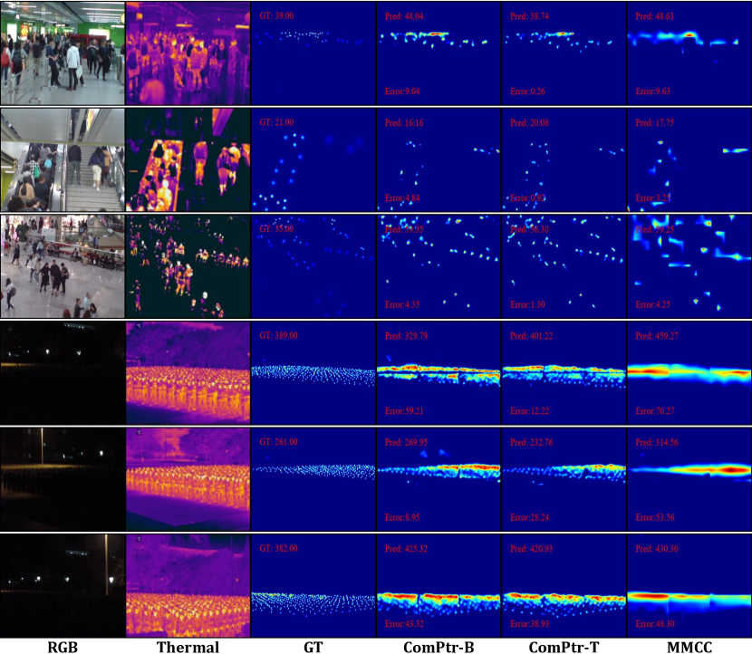
Figure 9: Visual comparison of samples corresponding to the bright scene in the top three rows, and to the low-brightness scene in the bottom three rows for RGB-T crowd counting. “GT”: The number of people annotated. “Pred”: The number estimated by the method. “Error”: The absolute error between “GT” and “Pred”.

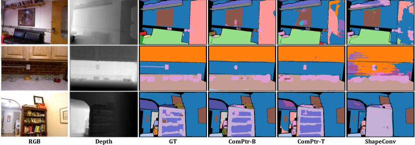
Figure 10: Visual comparison for RGB-D semantic segmentation.

4.5 RGB-D Semantic Segmentation (RGB-D SS)

Datasets. We also conduct extended experiments and analysis on the popular indoor RGB-D SS benchmark, NYU-Depth V2 dataset with 40 classes [9]. It contains 1449 pairs of RGB-D images with the shape of $480\times 640$, which is captured in the indoor scene. It is a representative and challenging RGB-D semantic segmentation dataset and includes complex and diverse indoor categories such as scene structures like walls and floors, furniture items like beds and chairs, and objects like lamps and bags. There are 795 image pairs for training and 654 image pairs for testing as [75, 29]. Following the practices and strategies of the existing works [79, 30, 29, 77, 28, 75], we employ some general data augmentation strategies as [75, 28], including random flipping, scaling and cropping, and set the number of epochs as 400, batch size as 8, initial learning rate as 0.00001, weight decay as 0.0001, and input size as $480\times 480$, respectively. The poly learning rate scheduler [88] with a warm-up stage and a factor of 0.9 is imposed on the AdamW optimizer [81].

Metrics. For RGB-D SS, three commonly used metrics, pixel accuracy (Pixel Acc.), mean accuracy (Mean Acc.), and mean region intersection over union (Mean IOU) are reported here. And they are defined as follows:

$$\mathrm{Pixel\ Acc.}=\frac{\sum_{i}N_{i\rightarrow i}}{\sum^{N_{cls}}_{j}\sum_{k}N_{j\rightarrow k}},$$ (16)

$$\mathrm{Mean\ Acc.}=\frac{1}{N_{cls}}\frac{\sum_{i}N_{i\rightarrow i}}{\sum_{k}N_{i\rightarrow k}},$$ (17)

$$\mathrm{Mean\ IOU}=\frac{1}{N_{cls}}\frac{\sum_{i}N_{i\rightarrow i}}{\sum_{k}N_{i\rightarrow k}+\sum_{k}N_{k\rightarrow i}-N_{i\rightarrow i}},$$ (18)

where $N_{i\rightarrow j}$ represents the number of pixels of class $i$ classified as class $j$ by the model and $N_{cls}$ is the number of classes in the dataset.

4.6 Comparison with State-of-the-Art Methods

We evaluate the competitiveness of our ComPtr by carefully comparing it with the state-of-the-art on different tasks. There are 12 models and variants from [10, 11, 14, 12, 43, 15, 13, 44, 12, 17] for RSCD, 11 methods for RGB-T CC which contains 6 single-modal methods [45, 46, 42, 47, 48, 49] retrained by [40] and 5 bi-modal methods [18, 5, 20, 19, 40], 15 methods [55, 21, 53, 56, 23, 57, 58, 59, 60, 24, 61, 62, 63, 25, 26] for RGB-D SOD, 10 methods [64, 66, 41, 65, 70, 67, 22, 69, 25, 26] for RGB-T SOD, and 13 methods [71, 73, 74, 72, 31, 75, 76, 28, 77, 29, 78, 30, 79] for RGB-D SS.

	RGBT-CC [5]					LEVIR-CD [3]					STEREO1000 [54]
$K$	GAME0 $\downarrow$	GAME1 $\downarrow$	GAME2 $\downarrow$	GAME3 $\downarrow$	RMSE $\downarrow$	Pre. $\uparrow$	Rec. $\uparrow$	F1 $\uparrow$	IOU $\uparrow$	OA $\uparrow$	$S_{m}$ $\uparrow$	$F^{\omega}_{\beta}$ $\uparrow$	MAE $\downarrow$	$E_{m}$ $\uparrow$	$F_{\beta}$ $\uparrow$
$1$	11.59	16.38	20.79	27.31	18.43	.9359	.9037	.9195	.8510	.9919	.9194	.8741	.0351	.9542	.9151
$2$	11.55	15.99	20.28	26.72	19.63	.9311	.9080	.9194	.8508	.9919	.9195	.8744	.0348	.9545	.9152
$4$	10.52	14.51	18.48	24.28	18.48	.9336	.9091	.9212	.8539	.9921	.9199	.8745	.0348	.9547	.9155
$8$	11.53	17.10	21.33	27.36	19.92	.9309	.9115	.9211	.8537	.9920	.9192	.8715	.0352	.9540	.9151
$16$	11.00	15.25	19.19	25.16	18.78	.9357	.9067	.9210	.8535	.9921	.9189	.8738	.0351	.9532	.9152
$\infty$	10.84	14.87	19.19	25.37	18.30	.9321	.9095	.9206	.8529	.9920	.9196	.8743	.0349	.9544	.9155
Std.	11.11	14.74	18.58	24.46	18.77	.9353	.9031	.9189	.8500	.9919	.9172	.8726	.0358	.9541	.9144

TABLE VII: Ablation on the number $K$ of the proxy prototypes in each attention layer. “$K=4$” is our final choice. “$\infty$”: With the same number of proxy prototypes as that of the input tokens. “Std.”: Dense interactive form of standard attention.

	RGBT-CC [5]					LEVIR-CD [3]					STEREO1000 [54]
Variants	GAME0 $\downarrow$	GAME1 $\downarrow$	GAME2 $\downarrow$	GAME3 $\downarrow$	RMSE $\downarrow$	Pre. $\uparrow$	Rec. $\uparrow$	F1 $\uparrow$	IOU $\uparrow$	$OA$ $\uparrow$	$S_{m}$ $\uparrow$	$F^{\omega}_{\beta}$ $\uparrow$	MAE $\downarrow$	$E_{m}$ $\uparrow$	$F_{\beta}$ $\uparrow$
ComPtr	10.52	14.51	18.48	24.28	18.48	.9336	.9091	.9212	.8539	.9921	.9199	.8745	.0348	.9547	.9155
$-$ CEB	11.14	14.91	18.72	24.43	19.71	.9308	.9059	.9182	.8488	.9918	.9126	.8628	.0378	.9475	.9146
$-$ DAB	11.22	15.43	19.50	25.68	19.52	.9317	.8942	.9126	.8392	.9913	.9043	.8579	.0411	.9453	.9095
$-$ Both	12.53	16.82	21.32	27.33	21.47	.9107	.8865	.8984	.8156	.9898	.8965	.8354	.0438	.9403	.8941
$-$ CompOps	11.20	15.90	20.05	26.20	19.32	.9266	.9083	.9174	.8473	.9917	.9143	.8672	.0366	.9479	.9146

TABLE VIII: Ablation on the proposed components in the complementary transformer. “$-$CEB”: Without the consistency enhancement block. “$-$DAB”: Without the difference awareness block. “$-$Both”: Baseline model which is a variant without the proposed blocks. “$-$CompOps”: ComPtr variant without the complementarity operation.

4.6.1 Quantitative Comparison

All comparisons are listed in Tab. II, Tab. III, Tab. IV, Tab. V, and Tab. VI. From the comparison in Tab. II, our method does not obtain the best results on Pre. and Rec., but achieves significant leading performance on F1 and IOU in the RSCD task. Compared with DMINet [17], “-T” version achieves a relative improvement of 1.55% F1 and 2.89% IOU on LEVIR-CD, and “-B” version yields performance gains of 1.05% F1 and 1.81% IOU on SYSU-CD. In RGB-T CC, ComPtr achieves an improvement of 0.38 GAME₀ and 0.31 RMSE over the recent [40] as shown in Tab. III. With respect to two bi-modal SOD methods, CAVER [26] and SwinNet [25], our performance is still superior, especially on DUTLF-Depth, SIP and STEREO1000 for RGB-D SOD in Tab. IV, and VT821 and VT1000 for RGB-T SOD in Tab. V. Besides, for more complex multi-class RGB-D SS in Tab. VI, our ComPtr-B achieves the best 55.5% mean IOU on NYU-Depth V2. The two versions, “-T” and “-B ”, perform differently on different tasks. There may be two underlying factors. On the one hand, it may be related to the different requirements of hyper-parameters during training for backbone with different volumes [89]. On the other hand, the different characteristics of these datasets result in different fitness for the swin architecture. Actually, to avoid over-engineering, we do not validate more parameter combinations and structural variants. And current results have demonstrated the generality of the proposed architecture and its adaptability to diverse task concepts, data forms, and object attributes.

4.6.2 Qualitative Comparison

In Fig. 6, Fig. 9, Fig. 7, Fig. 8, and Fig. 10, we visualize the prediction maps of the proposed model and several state-of-the-art methods. In addition to the results of our method, those of some recent methods with publicly available weight parameters or predictions are also listed. Visually, the results of our algorithm are much closer to the ground truth, and also adapt well to the complex examples shown here. For example, in the face of dense small buildings and independent large buildings in Fig. 6, and strong background interference in Fig. 7 and Fig. 8, our algorithm performs more robustly. For the prediction results of the RGB-T CC task in Fig. 9, ours has a smaller absolute error compared to MMCC [40]’s. It is also worth noting that our method still shows good crowd counting performance even in low-light scenarios due to the assistance of thermal infrared images. Besides, as shown in Fig. 10 for RGB-D SS, the predictions of our approaches also exhibit better intra-class consistency and inter-class differentiation. These effects can be attributed to the generality of the concept of complementarity for these tasks and the effectiveness of component design based on consistency and difference.

4.7 Ablation Studies

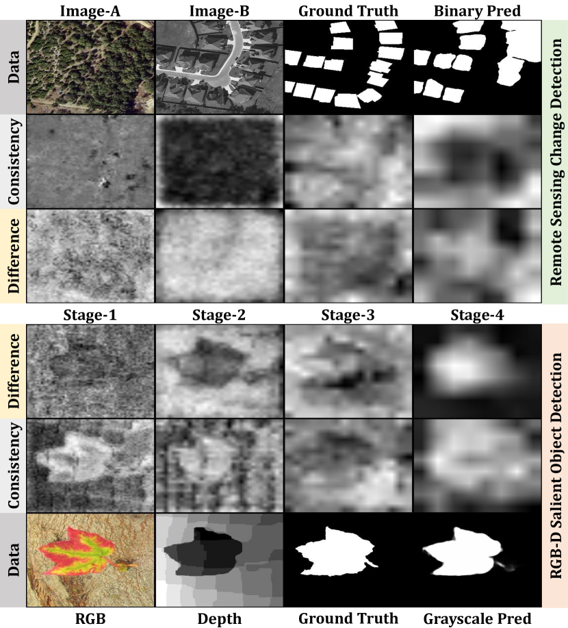
Figure 11: Averaged source feature maps in consistency enhancement and difference awareness blocks from different stages. These maps are obtained using bilinear interpolation after being averaged along the channels.

A series of ablation studies are presented in this section to reveal how the proposed components affect the final performance of the model. These experiments are constructed on three representative tasks, RGB-T CC, RSCD and RGB-D SOD, with large-scale datasets of various forms and attributes, where we take Swin-T [2] as the backbone.

4.7.1 Number of Proxy Prototypes

The number of proxy prototypes is an important hyper-parameter of the proposed ADA. To simplify the design process, the current version of the model uses the same number of prototypes in both types of embedded components. We set five small constant values $\{1,2,4,8,16\}$ for $K$ as candidates and record the performance of the five variants in Tab. VII on three different tasks, RGB-T CC, RSCD and RGB-D SOD, respectively. As we can see from the results, the sensitivity to $K$ varies across tasks. RSCD and RGB-D SOD tasks are relatively more robust to the value of $K$. Considering the balance of performance across tasks, we choose $K=4$ as the final setting. Besides, we also supplement two special cases, namely “$K=\infty$” where the value of $K$ is consistent with the number of input tokens and “Std.” where the proposed ADA is replaced with the full standard attention that also integrates CompOps for a reasonable comparison. Notably, the version $K=4$ surpasses the two benchmark versions, reflecting the potential of more compact representations for consistency and difference modelling. From the complexity statistics of different variants in Fig. 5, we can see that the proposed strategy based on the information aggregation mediated by a small number of prototypes can effectively save the computational budget of the inference process, which actually holds true for the training phase as well, and improve the parallel efficiency of the model.

4.7.2 Effectiveness of Proposed Components

To verify the effectiveness of the proposed components, we remove all complementarity operations, CEBs and DABs, respectively, and evaluate these variants on the three datasets from different tasks, RGB-T CC, RSCD, and RGB-D SOD. The results in Tab. VIII demonstrate that these components provide a positive gain for the performance of the final model. Besides, there is an interesting observation that removing the difference component causes significant performance degradation. This highlights the importance of difference information for bi-source tasks. At the same time, the consistency component also reflects the positive effect.

4.7.3 Feature Analysis

To better understand the behavior of the proposed components, the analysis is carried out in dense multi-object scenario and sparse single-object scenario. And the corresponding source features are visualized in Fig. 11. It is clear that the two operations play complementary roles in different stages. In the shallow layer (Stage-1&2), the detailed information from the difference operation and the object cues from the consistency operation are paid special attention. And in the deep layer (Stage-3&4), the two operations converge to the location of the object of interest, which is more obvious in the RGB-D SOD task. Besides, in RSCD, it can be seen that the difference maps in the shallow features almost cover the whole image, which reflects the dependence of this task on the attribute.

5 Conclusion

In this paper, we design a simple yet effective task-generic framework, ComPtr, from the concept of complementarity. It is common in bi-source information interaction for diverse dense prediction tasks with significantly different data patterns. From the perspective of consistency and difference, we design the consistency enhancement block and the difference awareness block respectively, which meet the needs of feature extraction and prediction decoding for complementary information. At the same time, we design an optimization strategy mediated by the proxy prototype, which effectively reduces the computational complexity of the global complementary information propagation process. Based on it, we construct a novel clustering-inspired aggregation-diffusion attention mechanism to improve the flexibility and scalability of the model. These simple yet effective designs make the proposed model no longer depend on task-specific data properties or forms, achieving a more general architecture. Extensive experiments on five diverse dense prediction tasks verify the effectiveness of the proposed method with superior performance to existing state-of-the-art competitors.

References

- [1] A. Dosovitskiy, L. Beyer, A. Kolesnikov, D. Weissenborn, X. Zhai, T. Unterthiner, M. Dehghani, M. Minderer, G. Heigold, S. Gelly, J. Uszkoreit, and N. Houlsby, “An image is worth 16x16 words: Transformers for image recognition at scale,” in ICLR, 2021.
- [2] Z. Liu, Y. Lin, Y. Cao, H. Hu, Y. Wei, Z. Zhang, S. Lin, and B. Guo, “Swin transformer: Hierarchical vision transformer using shifted windows,” in ICCV, 2021.
- [3] H. Chen and Z. Shi, “A spatial-temporal attention-based method and a new dataset for remote sensing image change detection,” RS, 2020.
- [4] Q. Shi, M. Liu, S. Li, X. Liu, F. Wang, and L. Zhang, “A deeply supervised attention metric-based network and an open aerial image dataset for remote sensing change detection,” TGRS, 2022.
- [5] H. Tang, Y. Wang, and L.-P. Chau, “Tafnet: A three-stream adaptive fusion network for rgb-t crowd counting,” in ISCAS, 2022.
- [6] T. Zhou, D.-P. Fan, M.-M. Cheng, J. Shen, and L. Shao, “Rgb-d salient object detection: A survey,” CVMJ, 2021.
- [7] A. Borji, M.-M. Cheng, Q. Hou, H. Jiang, and J. Li, “Salient object detection: A survey,” CVMJ, 2014.
- [8] W. Wang, Q. Lai, H. Fu, J. Shen, H. Ling, and R. Yang, “Salient object detection in the deep learning era: An in-depth survey,” TPAMI, 2021.
- [9] S. Gupta, P. Arbelaez, and J. Malik, “Perceptual organization and recognition of indoor scenes from rgb-d images,” in CVPR, 2013.
- [10] R. Caye Daudt, B. Le Saux, and A. Boulch, “Fully convolutional siamese networks for change detection,” in ICIP, 2018.
- [11] R. Caye Daudt, B. Le Saux, A. Boulch, and Y. Gousseau, “Multitask learning for large-scale semantic change detection,” CVIU, 2019.
- [12] Y. Liu, C. Pang, Z. Zhan, X. Zhang, and X. Yang, “Building change detection for remote sensing images using a dual-task constrained deep siamese convolutional network model,” LGRS, 2021.
- [13] B. Bai, W. Fu, T. Lu, and S. Li, “Edge-guided recurrent convolutional neural network for multitemporal remote sensing image building change detection,” TGRS, 2022.
- [14] C. Zhang, P. Yue, D. Tapete, L. Jiang, B. Shangguan, L. Huang, and G. Liu, “A deeply supervised image fusion network for change detection in high resolution bi-temporal remote sensing images,” JPRS, 2020.
- [15] H. Chen, Z. Qi, and Z. Shi, “Remote sensing image change detection with transformers,” TGRS, 2022.
- [16] Y. Feng, H. Xu, J. Jiang, H. Liu, and J. Zheng, “Icif-net: Intra-scale cross-interaction and inter-scale feature fusion network for bitemporal remote sensing images change detection,” TGRS, 2022.
- [17] Y. Feng, J. Jiang, H. Xu, and J. Zheng, “Change detection on remote sensing images using dual-branch multilevel intertemporal network,” TGRS, 2023.
- [18] L. Liu, J. Chen, H. Wu, G. Li, C. Li, and L. Lin, “Cross-modal collaborative representation learning and a large-scale rgbt benchmark for crowd counting,” in CVPR, 2021.
- [19] W. Zhou, Y. Pan, J. Lei, L. Ye, and L. Yu, “Defnet: Dual-branch enhanced feature fusion network for rgb-t crowd counting,” TITS, 2022.
- [20] Z. Wu, L. Liu, Y. Zhang, M. Mao, L. Lin, and G. Li, “Multimodal crowd counting with mutual attention transformers,” in ICME, 2022.
- [21] Y. Pang, L. Zhang, X. Zhao, and H. Lu, “Hierarchical dynamic filtering network for rgb-d salient object detection,” in ECCV, 2020.
- [22] W. Zhou, Q. Guo, J. Lei, L. Yu, and J.-N. Hwang, “Ecffnet: Effective and consistent feature fusion network for rgb-t salient object detection,” TCSVT, 2022.
- [23] Z. Liu, Y. Wang, Z. Tu, Y. Xiao, and B. Tang, “Tritransnet: Rgb-d salient object detection with a triplet transformer embedding network,” in ACM MM, 2021.
- [24] N. Liu, N. Zhang, K. Wan, L. Shao, and J. Han, “Visual saliency transformer,” in ICCV, 2021.
- [25] Z. Liu, Y. Tan, Q. He, and Y. Xiao, “Swinnet: Swin transformer drives edge-aware rgb-d and rgb-t salient object detection,” TCSVT, 2022.
- [26] Y. Pang, X. Zhao, L. Zhang, and H. Lu, “Caver: Cross-modal view-mixed transformer for bi-modal salient object detection,” TIP, 2023.
- [27] Y. Chen, T. Mensink, and E. Gavves, “3d neighborhood convolution: Learning depth-aware features for rgb-d and rgb semantic segmentation,” in 3DV, 2019.
- [28] L.-Z. Chen, Z. Lin, Z. Wang, Y.-L. Yang, and M.-M. Cheng, “Spatial information guided convolution for real-time rgbd semantic segmentation,” TIP, 2021.
- [29] J. Cao, H. Leng, D. Lischinski, D. Cohen-Or, C. Tu, and Y. Li, “Shapeconv: Shape-aware convolutional layer for indoor rgb-d semantic segmentation,” in ICCV, 2021.
- [30] L. Bai, J. Yang, C. Tian, Y. Sun, M. Mao, Y. Xu, and W. Xu, “Dcanet: Differential convolution attention network for rgb-d semantic segmentation,” 2022.
- [31] X. Qi, R. Liao, J. Jia, S. Fidler, and R. Urtasun, “3d graph neural networks for rgbd semantic segmentation,” in ICCV, 2017.
- [32] J. Devlin, M.-W. Chang, K. Lee, and K. Toutanova, “Bert: Pre-training of deep bidirectional transformers for language understanding,” in NAACL, 2019.
- [33] T. Brown, B. Mann, N. Ryder, M. Subbiah, J. D. Kaplan, P. Dhariwal, A. Neelakantan, P. Shyam, G. Sastry, A. Askell, S. Agarwal, A. Herbert-Voss, G. Krueger, T. Henighan, R. Child, A. Ramesh, D. Ziegler, J. Wu, C. Winter, C. Hesse, M. Chen, E. Sigler, M. Litwin, S. Gray, B. Chess, J. Clark, C. Berner, S. McCandlish, A. Radford, I. Sutskever, and D. Amodei, “Language models are few-shot learners,” in NIPS, 2020.
- [34] B. Yan, Y. Jiang, P. Sun, D. Wang, Z. Yuan, P. Luo, and H. Lu, “Towards grand unification of object tracking,” in ECCV, 2022.
- [35] F. Yu and V. Koltun, “Multi-scale context aggregation by dilated convolutions,” in ICLR, 2016.
- [36] L.-C. Chen, G. Papandreou, I. Kokkinos, K. Murphy, and A. L. Yuille, “Deeplab: Semantic image segmentation with deep convolutional nets, atrous convolution, and fully connected crfs,” TPAMI, 2017.
- [37] C. Peng, X. Zhang, G. Yu, G. Luo, and J. Sun, “Large kernel matters — improve semantic segmentation by global convolutional network,” in CVPR, 2017.
- [38] X. Wang, R. Girshick, A. Gupta, and K. He, “Non-local neural networks,” in CVPR, 2018.
- [39] Z. Chen, Y. Duan, W. Wang, J. He, T. Lu, J. Dai, and Y. Qiao, “Vision transformer adapter for dense predictions,” 2023.
- [40] Z. Liu, W. Wu, Y. Tan, and G. Zhang, “Rgb-t multi-modal crowd counting based on transformer,” 2022.
- [41] Z. Tu, Y. Ma, Z. Li, C. Li, J. Xu, and Y. Liu, “Rgbt salient object detection: A large-scale dataset and benchmark,” ArXiv, 2020.
- [42] B. Wang, H. Liu, D. Samaras, and M. H. Nguyen, “Distribution matching for crowd counting,” in NIPS, 2020.
- [43] S. Fang, K. Li, J. Shao, and Z. Li, “Snunet-cd: A densely connected siamese network for change detection of vhr images,” LGRS, 2022.
- [44] Q. Guo, J. Zhang, S. Zhu, C. Zhong, and Y. Zhang, “Deep multiscale siamese network with parallel convolutional structure and self-attention for change detection,” TGRS, 2022.
- [45] Y. Li, X. Zhang, and D. Chen, “Csrnet: Dilated convolutional neural networks for understanding the highly congested scenes,” in CVPR, 2018.
- [46] Z. Ma, X. Wei, X. Hong, and Y. Gong, “Bayesian loss for crowd count estimation with point supervision,” in ICCV, 2019.
- [47] Q. Song, C. Wang, Z. Jiang, Y. Wang, Y. Tai, C. Wang, J. Li, F. Huang, and Y. Wu, “Rethinking counting and localization in crowds: A purely point-based framework,” in ICCV, 2021.
- [48] L. Rong and C. Li, “Coarse- and fine-grained attention network with background-aware loss for crowd density map estimation,” in WACV, 2021.
- [49] H. Lin, Z. Ma, R. Ji, Y. Wang, and X. Hong, “Boosting crowd counting via multifaceted attention,” in CVPR, 2022.
- [50] Y. Piao, W. Ji, J. Li, M. Zhang, and H. Lu, “Depth-induced multi-scale recurrent attention network for saliency detection,” in ICCV, 2019.
- [51] R. Ju, Y. Liu, T. Ren, L. Ge, and G. Wu, “Depth-aware salient object detection using anisotropic center-surround difference,” SPIC, 2015.
- [52] H. Peng, B. Li, W. Xiong, W. Hu, and R. Ji, “Rgbd salient object detection: A benchmark and algorithms,” in ECCV, 2014.
- [53] D.-P. Fan, Z. Lin, Z. Zhang, M. Zhu, and M.-M. Cheng, “Rethinking rgb-d salient object detection: Models, data sets, and large-scale benchmarks,” TNNLS, 2021.
- [54] Y. Niu, Y. Geng, X. Li, and F. Liu, “Leveraging stereopsis for saliency analysis,” in CVPR, 2012.
- [55] K. Fu, D.-P. Fan, G.-P. Ji, Q. Zhao, J. Shen, and C. Zhu, “Siamese network for rgb-d salient object detection and beyond,” TPAMI, 2022.
- [56] Q. Chen, Z. Liu, Y. X. Zhang, K. Fu, Q. Zhao, and H. Du, “Rgb-d salient object detection via 3d convolutional neural networks,” in AAAI, 2021.
- [57] W. Ji, J. Li, S. Yu, M. Zhang, Y. Piao, S. Yao, Q. Bi, K. Ma, Y. Zheng, H. Lu, and L. Cheng, “Calibrated rgb-d salient object detection,” in CVPR, 2021.
- [58] P. Sun, W. Zhang, H. Wang, S. Li, and X. Li, “Deep rgb-d saliency detection with depth-sensitive attention and automatic multi-modal fusion,” in CVPR, 2021.
- [59] J. Zhang, D.-P. Fan, Y. Dai, X. Yu, Y. Zhong, N. Barnes, and L. Shao, “Rgb-d saliency detection via cascaded mutual information minimization,” in ICCV, 2021.
- [60] T. Zhou, D.-P. Fan, G. Chen, Y. Zhou, and H. Fu, “Specificity-preserving rgb-d saliency detection,” CVMJ, 2022.
- [61] G. Li, Z. Liu, M. Chen, Z. Bai, W. Lin, and H. Ling, “Hierarchical alternate interaction network for rgb-d salient object detection,” TIP, 2021.
- [62] W. Zhou, Y. Zhu, J. Lei, J. Wan, and L. Yu, “Ccafnet: Crossflow and cross-scale adaptive fusion network for detecting salient objects in rgb-d images,” TMM, 2021.
- [63] F. Wang, J. Pan, S. Xu, and J. Tang, “Learning discriminative cross-modality features for rgb-d saliency detection,” TIP, 2022.
- [64] G. Wang, C. Li, Y. Ma, A. Zheng, J. Tang, and B. Luo, “Rgb-t saliency detection benchmark: Dataset, baselines, analysis and a novel approach,” in IGTA, 2018.
- [65] Z. Tu, T. Xia, C. Li, X. Wang, Y. Ma, and J. Tang, “Rgb-t image saliency detection via collaborative graph learning,” TMM, 2020.
- [66] Z. Tu, T. Xia, C. Li, Y. Lu, and J. Tang, “M3s-nir: Multi-modal multi-scale noise-insensitive ranking for rgb-t saliency detection,” in MIPR, 2019.
- [67] F. Huo, X. Zhu, L. Zhang, Q. Liu, and Y. Shu, “Efficient context-guided stacked refinement network for rgb-t salient object detection,” TCSVT, 2021.
- [68] S. Mehta, M. Rastegari, L. Shapiro, and H. Hajishirzi, “Espnetv2: A light-weight, power efficient, and general purpose convolutional neural network,” in CVPR, 2019.
- [69] Z. Tu, Z. Li, C. Li, Y. Lang, and J. Tang, “Multi-interactive dual-decoder for rgb-thermal salient object detection,” TIP, 2021.
- [70] J. Wang, K. Song, Y. Bao, L. Huang, and Y. Yan, “Cgfnet: Cross-guided fusion network for rgb-t salient object detection,” Tcsvt, 2021.
- [71] Y. Cheng, R. Cai, Z. Li, X. Zhao, and K. Huang, “Locality-sensitive deconvolution networks with gated fusion for rgb-d indoor semantic segmentation,” in CVPR, 2017.
- [72] S. Lee, S.-J. Park, and K.-S. Hong, “Rdfnet: Rgb-d multi-level residual feature fusion for indoor semantic segmentation,” in ICCV, 2017.
- [73] F. Fooladgar and S. Kasaei, “Multi-modal attention-based fusion model for semantic segmentation of rgb-depth images,” 2019.
- [74] X. Hu, K. Yang, L. Fei, and K. Wang, “Acnet: Attention based network to exploit complementary features for rgbd semantic segmentation,” in ICIP, 2019.
- [75] X. Chen, K.-Y. Lin, J. Wang, W. Wu, C. Qian, H. Li, and G. Zeng, “Bi-directional cross-modality feature propagation with separation-and-aggregation gate for rgb-d semantic segmentation,” in ECCV, 2020.
- [76] Y. Xing, J. Wang, and G. Zeng, “Malleable 2.5d convolution: Learning receptive fields along the depth-axis for rgb-d scene parsing,” in ECCV, 2020.
- [77] G. Zhang, J.-H. Xue, P. Xie, S. Yang, and G. Wang, “Non-local aggregation for rgb-d semantic segmentation,” SPL, 2021.
- [78] S. Borse, Y. Wang, Y. Zhang, and F. Porikli, “Inverseform: A loss function for structured boundary-aware segmentation,” in CVPR, 2021.
- [79] J. Yang, L. Bai, Y. Sun, C. Tian, M. Mao, and G. Wang, “Pixel difference convolutional network for rgb-d semantic segmentation,” 2023.
- [80] J. Deng, W. Dong, R. Socher, L.-J. Li, K. Li, and L. Fei-Fei, “Imagenet: A large-scale hierarchical image database,” CVPR, 2009.
- [81] I. Loshchilov and F. Hutter, “Decoupled weight decay regularization,” in ICLR, 2019.
- [82] L. N. Smith and N. Topin, “Super-convergence: Very fast training of neural networks using large learning rates,” in Artificial Intelligence and Machine Learning for Multi-Domain Operations Applications, 2019.
- [83] R. Guerrero-Gómez-Olmedo, B. Torre-Jiménez, R. López-Sastre, S. Maldonado-Bascón, and D. Oñoro-Rubio, “Extremely overlapping vehicle counting,” in PRIA, 2015.
- [84] D.-P. Fan, M.-M. Cheng, Y. Liu, T. Li, and A. Borji, “Structure-measure: A new way to evaluate foreground maps,” in ICCV, 2017.
- [85] R. Achanta, S. Hemami, F. Estrada, and S. Süsstrunk, “Frequency-tuned salient region detection,” in CVPR, 2009.
- [86] D.-P. Fan, C. Gong, Y. Cao, B. Ren, M.-M. Cheng, and A. Borji, “Enhanced-alignment measure for binary foreground map evaluation,” in IJCAI, 2018.
- [87] R. Margolin, L. Zelnik-Manor, and A. Tal, “How to evaluate foreground maps?” in CVPR, 2014.
- [88] W. Liu, A. Rabinovich, and A. C. Berg, “Parsenet: Looking wider to see better,” arXiv e-prints, 2015.
- [89] J. Kaplan, S. McCandlish, T. Henighan, T. B. Brown, B. Chess, R. Child, S. Gray, A. Radford, J. Wu, and D. Amodei, “Scaling laws for neural language models,” 2020.