Scaling Laws for Imitation Learning in NetHack

Abstract

Imitation Learning (IL) is one of the most widely used methods in machine learning. Yet, while powerful, many works find it is often not able to fully recover the underlying expert behavior [1, 2, 3]. However, none of these works deeply investigate the role of scaling up the model and data size. Inspired by recent work in Natural Language Processing (NLP) [4, 5] where “scaling up” has resulted in increasingly more capable LLMs, we investigate whether carefully scaling up model and data size can bring similar improvements in the imitation learning setting. To demonstrate our findings, we focus on the game of NetHack, a challenging environment featuring procedural generation, stochasticity, long-term dependencies, and partial observability. We find IL loss and mean return scale smoothly with the compute budget and are strongly correlated, resulting in power laws for training compute-optimal IL agents with respect to model size and number of samples. We forecast and train several NetHack agents with IL and find they outperform prior state-of-the-art by at least 2x in all settings. Our work both demonstrates the scaling behavior of imitation learning in a challenging domain, as well as the viability of scaling up current approaches for increasingly capable agents in NetHack, a game that remains elusively hard for current AI systems.

1 Introduction

While conceptually simple, imitation learning has powered some of the most impressive feats of AI in recent years. AlphaGo [6] used imitation on human Go games to bootstrap its Reinforcement Learning (RL) policy. Cicero, an agent that can play the challenging game of Diplomacy, used an IL-based policy as an anchor to guide planning [3]. Beyond games, SayCan [7], a system that grounds language in robotic affordances, used IL to train the individual “atomic" skills in its robotic system.

Despite its prevalence, several works have pointed out some of the limitations of IL. De Haan et al. [2] and Wen et al. [1] call out the issue of causal confusion, where the IL policy relies on spurious correlations to achieve high training and held-out accuracy, but performs far worse than the data-generating policy when deployed in the environment. Jacob et al. [3] have mentioned similar issues for policies learning from human games: they consistenly underperform the data-generating policy. However, in many of these works, the role of model and data size is not deeply investigated. This is especially striking considering the increasingly impressive capabilities that recent language models have exhibited, mostly as a consequence of scale. In a series of papers trying to characterize these improvements with scale starting with Kaplan et al. [4], it has been shown language modeling loss (i.e. cross-entropy) scales smoothly with model size and number of training tokens [5]. If we think of language models as essentially performing “imitation learning" on text, then a natural next question is whether some of these results extend to IL-based agents in the control domain, and whether scale could provide similar benefits and alleviate some of the issues mentioned earlier on.

In this paper, we ask the following question: How does compute in terms of model and data size affect the performance of agents trained with imitation learning? To start answering this question, we focus on the challenging game of NetHack, a roguelike video game released in 1987. NetHack is an especially well-suited and interesting domain to study for several reasons. First, it is procedurally generated and highly stochastic, disqualifying approaches relying heavily on memorization instead of generalization, such as Go-Explore [8]. Second, the game is partially observed, requiring the use of memory, potentially for thousands of steps due to the game’s long-term dependencies. Finally, the game is extremely challenging for current AI systems, with current agents reaching scores nowhere close to average human performance. The current best agent on NetHack is a purely rule-based system called AutoAscend [10], with RL approaches lagging behind [9, 11, 12, 13]. Even just recovering this system is hard, with Hambro et al. [9] reporting that the best neural agents achieve less than 10% of the system’s mean return in the environment, causing the authors to call for significant research advances. We instead investigate whether simply scaling up BC can close this gap.

Contributions.

We train a suite of neural NetHack agents with different model sizes using BC to imitate AutoAscend and analyze the loss and mean return isoFLOP profiles. We find the optimal cross-entropy loss scales as a power law in the compute budget, and we use two different methods to derive scaling laws for the loss-optimal model and data sizes. We then relate the cross-entropy loss of our trained BC agents to their respective mean return when rolled out in the environment, and find that the mean return follows a power law with respect to the optimal cross-entropy loss, showing improvements in loss predictably translate in better performing agents. We use our two scaling law derivations to forecast the training requirements of a compute-optimal neural BC agent. These forecasts are then used to train an agent which outperforms prior neural NetHack agents by 2x in all settings, showing scale can provide dramatic improvements in performance. We extend our results to the RL setting, where we also train a suite of NetHack agents using IMPALA [14] on the NetHackScore-v0 environment and again find that model and data size scale as power laws in the compute budget. Finally, we forecast the compute requirements for training an RL agent from scratch to achieve average human-level performance, though we do not train such agent.

Our results demonstrate that, similarly to language models, the improvements in imitation and reinforcement learning performance in the challenging domain of NetHack can be described by clean power laws. This suggests carefully scaling up model and data size can provide a promising path towards increasingly capable NetHack agents, as well as boost performance in other imitation learning settings.

2 Preliminaries

We now introduce the formal setup for behavioral cloning and reinforcement learning. In both cases, we assume the environment can be described by a Partially Observable Markov Decision Process (POMDP) $\langle S,T,A,O,R,\gamma\rangle$, with states $S$, transition function $T$, action set $A$, possible observation emissions $O$, reward function $R(s,a)$, and discount factor $\gamma$.

Behavioral cloning.

In this setup, we don’t assume access to the rewards but instead have access to a dataset $\mathcal{D}$ consisting of trajectories $\tau=(s_{0},a_{0},s_{1},a_{1},\ldots)$ of states and actions. These trajectories can be generated by multiple (possibly sub-optimal) demonstrators acting in the environment. However, in this work, they are assumed to all come from the same expert policy $\pi$. The goal is to recover this expert policy. To do this, a learner $\pi_{\theta}$ will optimize the following cross-entropy loss:

$$\mathcal{L}(\theta)=-\mathbb{E}_{(h_{t},a_{t})\sim\mathcal{D}}\left[\log\pi_{\theta}(a_{t}|h_{t})\right],$$ (1)

where $h_{t}$ can include part or the entirety of the history of past states and actions.

Reinforcement learning.

In this setup, we do assume access to the environment rewards and aim to explicitly maximize their cumulative sum over time, i.e. $V^{\pi}=\mathbb{E}\left[\sum_{t=0}^{H}R_{t}(s_{t},a_{t})\right]$, where the expectation is taken over the policy $\pi$ and the underlying POMDP (i.e. initial state and transition distribution). We only focus on policy gradient methods, which use a parameterized policy $\pi_{\theta}$ to directly optimize $V^{\pi_{\theta}}$ using the policy gradient:

$$\nabla V^{\pi_{\theta}}(\mu)=\frac{1}{1-\gamma}\mathbb{E}_{s\sim d^{\pi_{\theta}}}\mathbb{E}_{a\sim\pi_{\theta}(\cdot|s)}\left[A^{\pi_{\theta}}(s,a)\nabla\log\pi_{\theta}(a|s)\right],$$ (2)

where $d^{\pi_{\theta}}$ is the state visitation measure, and $A^{\pi_{\theta}}$ is the advantage function.

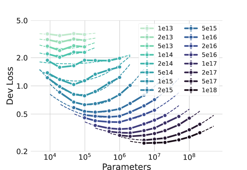
(a) IsoFLOP curves

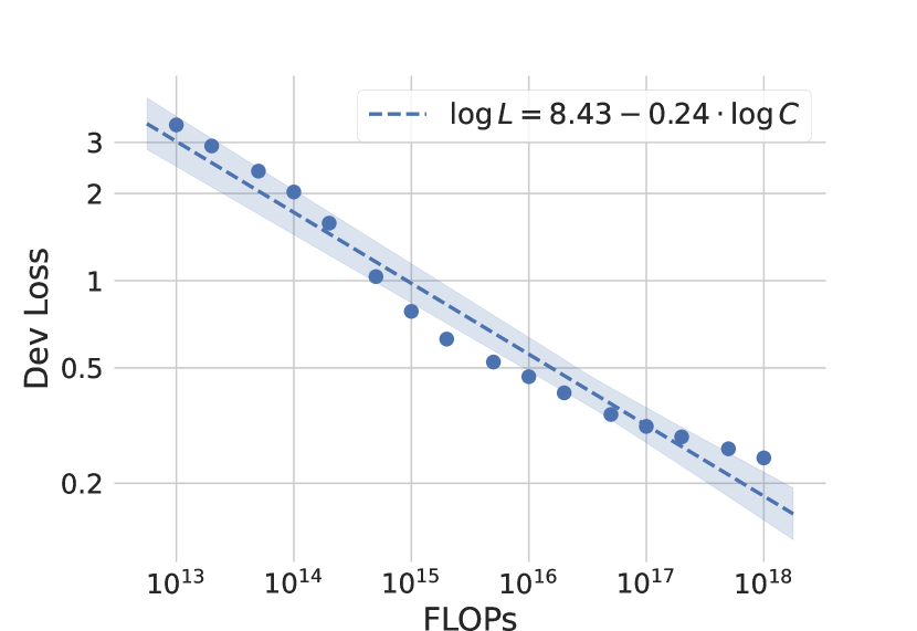
(b) Optimal loss vs. FLOPs

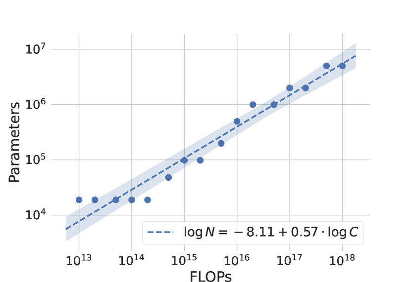
(c) Optimal parameters vs. FLOPs

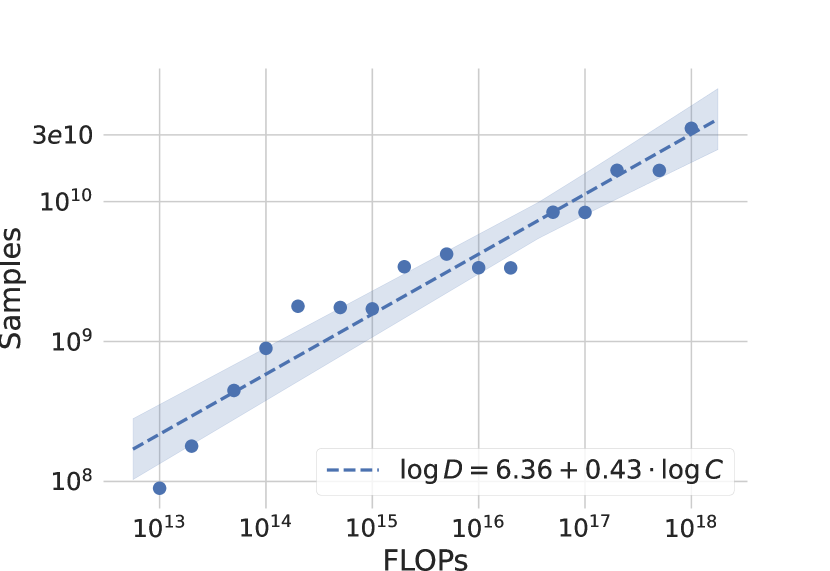
(d) Optimal samples vs. FLOPs

Figure 1: BC loss scaling. We train a wide range of model sizes across several orders of magnitudes of FLOP budgets. We plot the validation loss for each model, with fitted parabolas per IsoFLOPs curve (a). We then regress the loss minima (b), the loss-optimal number of parameters (c), and the loss-optimal number of samples (d) on their corresponding FLOP budgets. We find all of them follow a clear power law trend.

3 Experimental setup

Whenever we report FLOP or parameter counts, we are referring to their effective counts, which we define as only including the parts of the network that are being scaled (similar to Hilton et al. [15], see Appendix E for full details). We analyzed the scaling behavior of neural NetHack agents in two different settings:

1. Behavioral cloning: We train LSTM-based agents on the NLD-AA dataset [9], mainly varying the width of the LSTM (see Appendix E). The total number of parameters ranged from 10k to 500M. While the original NLD-AA dataset already contains around 3B samples, we extended the dataset to around 60B samples (NLD-AA-L) and 150B samples (NLD-AA-XL) by collecting more rollouts from AutoAscend (i.e. the data-generating policy). NLD-AA-L is used for the results in 1(a), while NLD-AA-XL is used for all our forecasting-based experiments.

2. Reinforcement learning: We train LSTM-based agents on the NetHackScore-v0 environment. NetHackScore-v0 features the full game of NetHack but has a reduced action space, starting character fixed to human monk, and automatic menu skipping. The total number of parameters ranged from 100k to 50M. We also experimented with the NetHackChallenge-v0 environment but found the results too noisy at the FLOP budgets we were able to run. However, we expect similar results will hold for this environment at larger FLOP budgets.

Please see Appendix F for details on all hyperparameters for all experiments.

4 Scaling up imitation learning

This section is structured as follows. We first investigate the role of model size and number of samples with respect to cross-entropy loss (subsection 4.1). While intuitively it feels like a lower loss should result in a better agent, we verify this by directly investigating the role of model size and number of samples with respect to the environment return (subsection 4.2), and relating these results to the loss results. In subsection 4.3, we then forecast a few model variants aimed to recover the underlying expert behavior. Finally, we also extend our analysis to the RL setting (section 5).

4.1 Scaling laws for BC loss

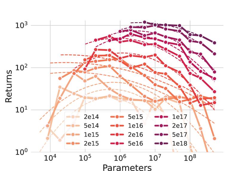
(a) IsoFLOP curves

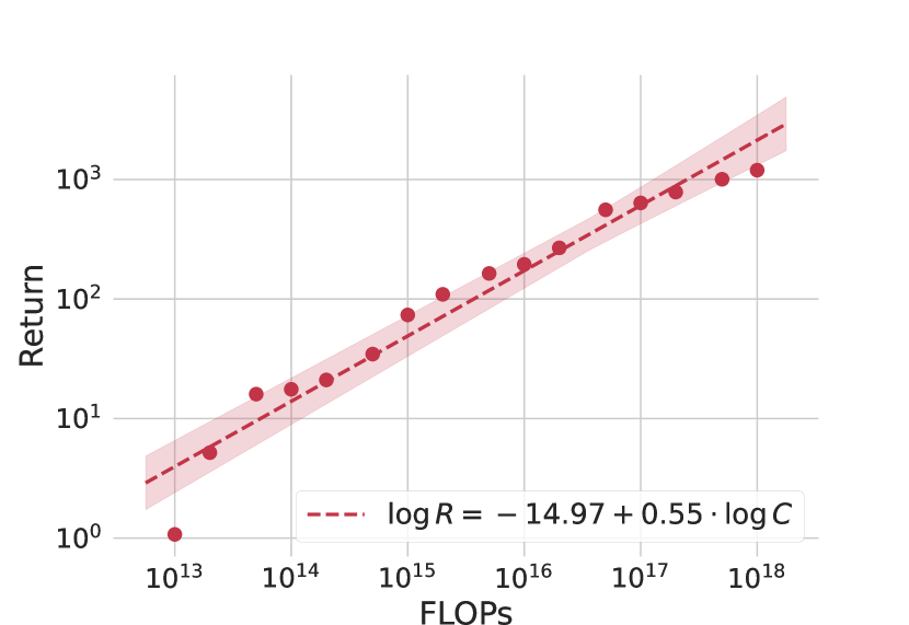
(b) Optimal return vs. FLOPs

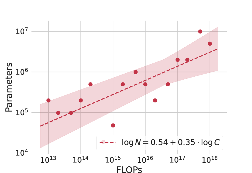
(c) Optimal parameters vs. FLOPs

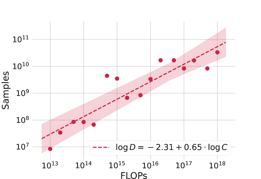
(d) Optimal samples vs. FLOPs

Figure 2: BC return scaling. We train a wide range of model sizes across several orders of magnitudes of FLOP budgets (same models as in 1(a)) and plot their average return in the environment (a). We left off the first four FLOP budgets as we found them to be especially noisy. We then regress the optimal returns (b), the return-optimal number of parameters (c), and the return-optimal number of samples (d) on their corresponding FLOP budgets. We find all of them follow a power law trend.

To investigate the role of model size and number of samples with respect to cross-entropy loss, we follow similar approaches to the ones used in Hoffmann et al. [5].

Approach #1: isoFLOP profiles.

We train 14 different model sizes, ranging from 10k to 500M, each with a FLOP budget of at least $1e13$ and up to $1e18$. We plot the loss evaluated on a held-out set of 85 trajectories against the parameter count for each FLOP budget (see Figure 1). Similarly to Hoffmann et al. [5], we observe clear parabolas with well-defined minima at the optimal model size for a given compute budget. We take these loss-optimal data points to fit three regressions: one that regresses the log parameters on the log FLOPs, another that regresses the log samples on the log FLOPs, and a final one that regresses the log loss on the log FLOPs. These regressions give rise to the following power laws (1(c), 1(d), and 1(b)):

$$N_{\mathrm{opt}}\propto C^{\alpha}\quad D_{\mathrm{opt}}\propto C^{\beta}\quad L_{\mathrm{opt}}\propto C^{\gamma},$$ (3)

where $N$ indicates the model size, $D$ the number of training samples, and $L$ the validation loss. We found $\alpha=0.57$, $\beta=0.43$, and $\gamma=-0.24$.

Approach #2: parametric fit.

Instead of only fitting the loss-optimal points as was done in approach #1 above, we now fit all points from 1(a) to the following quadratic form:

$$\log\hat{L}(N,D)=\beta_{0}+\beta_{N}\log N+\beta_{D}\log D+\beta_{N^{2}}(\log N)^{2}+\beta_{ND}\log N\log D+\beta_{D^{2}}(\log D)^{2}.$$ (4)

If we only look at the linear terms here, we notice that this loss has the form of a Cobb-Douglas production function:

$$\hat{L}(N,D)=\exp(\beta_{0})\times N^{\beta_{N}}\times D^{\beta_{D}},$$ (5)

where we can think of parameters $N$ and samples $D$ as inputs that affect how much output (i.e. loss) gets produced. We then take the functional form in Equation 4 and minimize the loss subject to the constraint that $\mathrm{FLOPs}(N,D)\approx 6ND$. To do this, we used the method of Lagrange multipliers to get the following functional forms for $N_{\mathrm{opt}}$ and $D_{\mathrm{opt}}$ (see Appendix A for full derivation):

$$N_{\mathrm{opt}}=G\left(\frac{C}{6}\right)^{\alpha},\quad D_{\mathrm{opt}}=G^{-1}\left(\frac{C}{6}\right)^{\beta},\quad\mathrm{where}\quad G=\exp\left(\frac{\beta_{D}-\beta_{N}}{2\beta_{D^{2}}-2\beta_{ND}+2\beta_{N^{2}}}\right).$$ (6)

We find that $\alpha=\frac{2\beta_{D^{2}}-\beta_{ND}}{2\beta_{D^{2}}-2\beta_{ND}+2\beta_{N^{2}}}=0.48$ and $\beta=\frac{2\beta_{N^{2}}-\beta_{ND}}{2\beta_{D^{2}}-2\beta_{ND}+2\beta_{N^{2}}}=0.52$.

Setting	IsoFLOP profiles		Parametric fit
	$\alpha$	$\beta$	$\alpha$	$\beta$
1. BC Loss	0.57 (0.50, 0.64)	0.43 (0.36, 0.50)	0.48 (0.47, 0.49)	0.52 (0.51, 0.53)
2. BC Return	0.35 (0.18, 0.52)	0.65 (0.48, 0.82)	0.34 (0.33, 0.35)	0.66 (0.65, 0.67)
3. RL Return	0.43 (0.25, 0.62)	0.56 (0.37, 0.75)	0.60 (0.59, 0.61)	0.40 (0.39, 0.41)

Table 1: Fitted power law coefficients. We list the scaling coefficients for model size ($\alpha$) and number of samples ($\beta$) for all three settings. 95% CIs are noted in parentheses, where the delta method was used for the parametric fit parameters (see Appendix G).

4.2 Scaling laws for BC return

Note that the analysis in the previous section was all in terms of cross-entropy loss. However, in the imitation learning setting, we almost never care directly about this quantity. Instead, we care about the performance of the resulting agent in the environment, measured by the average return. To investigate how this quantity scales, we roll out every model from 1(a) in the NetHack environment and average their score across 1k rollouts each (see 2(a)). We then follow a similar procedure as in subsection 4.1 and perform the same three regressions, giving rise to the following power laws (2(c), 2(d), and 2(b)):

$$N_{\mathrm{opt}}\propto C^{\alpha}\quad D_{\mathrm{opt}}\propto C^{\beta}\quad R_{\mathrm{opt}}\propto C^{\gamma},$$ (7)

where we found $\alpha=0.35$, $\beta=0.65$, and $\gamma=0.55$.

Additionally, we can take the functional form in Equation 4 and simply replace loss with mean return. We can then solve the same constrained optimization problem resulting in the exact same expressions as found in Equation 6. After fitting, we find $\alpha=0.34{}$ and $\beta=0.66$.

To investigate the relationship between loss and mean return, we regress the loss-optimal log returns (from 1(a)) on the corresponding log loss values. We find a power law of the form $R_{\mathrm{opt}}\propto L_{\mathrm{opt}}^{\delta}$, as shown in 3(a), where $\delta=-2.42$. The fit in the figure shows optimal loss and mean return are highly correlated, indicating we can expect return to increase smoothly as we make improvements in loss, rather than showing sudden jumps.

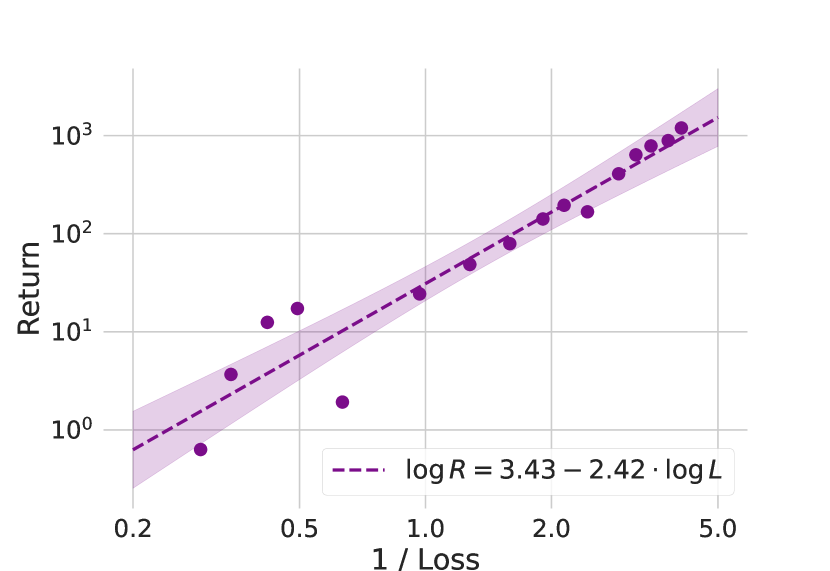
(a) Return vs. optimal loss

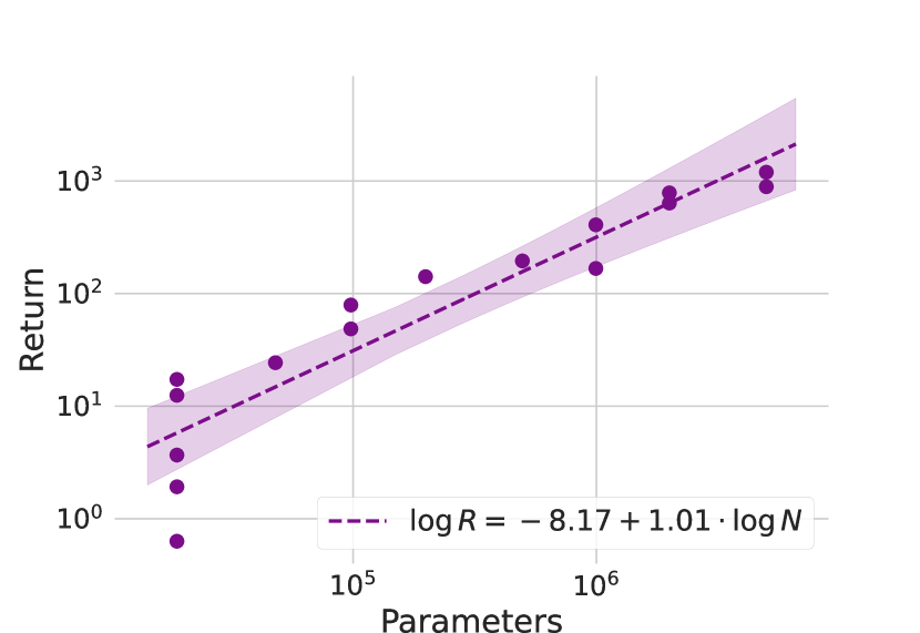
(b) Return vs. loss-optimal params

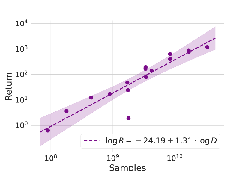
(c) Return vs. loss-optimal samples

Figure 3: BC return-loss relation. We investigate the relationship between the loss of a BC agent and its corresponding return. In (a), we show the optimal loss and mean return are highly correlated. We then regress the return directly on the loss-optimal parameters (b) and samples (c).

4.3 Forecasting compute-optimal BC agents

The isoFLOP profiles and power laws shown in Figure 1 and Figure 2 allow us to estimate the compute-optimal number of samples and parameters needed to train an agent that recovers the expert’s (AutoAscend) behavior. To do this, we follow two approaches:

1. Using loss isoFLOP profiles. We first plug in $R=10k$ into the regression in 3(a) to solve for $L_{10k}$, the loss needed for a score of $10k$. Then, we plug $L_{10k}$ into the regression in 1(b) to get $C_{10k}$, the FLOPs needed to recover a score of $10k$. Then we find the optimal parameters and samples using 1(c) and 1(d).

2. Using parametric fit. We take $C_{10k}$ from above, and use Equation 6 found by the parametric fit to solve for the parameters $N$ and samples $D$.

Results for both methods can be found in 2(a). We find that the second approach predicts a smaller model size but more samples, similar to findings in Hoffmann et al. [5]. In Appendix H, we also perform rolling time series cross-validation to evaluate one-step ahead forecasting performance.

Based on early forecasting fits, we train a 30M parameter model for 115B samples. The mean return and comparison with prior work can be found in 2(b). While we do not recover the underlying expert behavior (score of 10k), we do find the resulting model gets a big boost in performance and outperforms prior state-of-the-art by 2x, both when using a random initial character (hardest setting) as well as when its kept fixed to human monk. There can be multiple reasons as to why we do not fully recover the expert. First, we may not haved tuned hyperparameters extensively enough. In particular, the hyperparameters for all isoFLOP curves were all kept fixed. Second, it is plausible we did not evaluate up to a high enough FLOP budget to more accurately capture the correct power law exponents. This may have caused us to underestimate the importance of model size.

Approach	Params	Samples
BC - Expert (10k)
1. IsoFLOP profiles	43M	144B
2. Parametric fit	17M	362B
RL - Avg. Human (127k)
1. IsoFLOP profiles	4.4B	13.2T
2. Parametric fit	67B	0.93T

(a) Model and data size predictions

	All	Human
Models	Random	Monk
Offline only
DQN-Offline [9]	0.0	0.0
CQL [9]	352	366
IQL [9]	171	267
BC (CDGPT5) [9, 10]	554	1059
BC (Transformer) [16]	1318	-
Scaled-BC (ours)	2740	5218
Offline + Online
Kickstarting + BC [9]	962	2090
APPO + BC [9]	1282	2809
APPO + BC [16]	1551	-
LDD∗ [12]	-	2100

(b) Score comparison

Table 2: Forecasting results. In (a), we use two different ways of forecasting a model trained with a compute-optimal number of parameters and samples that attempts to (1) recover the underlying expert score (in the BC setting) or (2) attain average human performance (in the RL setting). In (b), we compare a model trained with BC using 30M parameters on 115B samples with previous models in the NetHackChallenge-v0 environment and find it matches or outperforms all of them on both randomized character initialization (harder) as well as initialized with human monk (easier). ^∗Exact scores not reported in original work. Scores from Hambro et al. [9] were adjusted to account for an error in their original evaluation code. See Appendix B for full results with standard errors.

5 Scaling up reinforcement learning

Several works in the past couple of years have attempted RL-based approaches for NetHack. The original NLE paper ran an IMPALA baseline [11], with follow-up works combining offline pretraining with online RL [9, 12]. However, none of these come close to ascension (i.e. winning the game). We investigate the role of model size and environment interactions for current RL methods using approaches 1 and 2 from subsection 4.1 applied to IMPALA.

IsoFLOP profiles.

We train 9 different model sizes ranging from 100k to 50M using IMPALA [14], each with a FLOP budget ranging from $1e13$ to $1e17$. For each of these models, we evaluate the model at the end of training by rolling it out 1k times in the environment and reporting the average return. While learning curves in RL tend to have high variance, we generally still find that compute-optimal models should increase both the number of parameters and number of environment interactions as the FLOP budgets are scaled up (see Figure 4). We also find that the NetHack game score varies smoothly with FLOPs and hence can be seen as a natural performance metric [15]. We again follow a similar procedure as in subsection 4.1 resulting in power laws as listed in Equation 7. We find $\alpha=0.43{}$, $\beta=0.56{}$, and $\gamma=0.32$.

Parametric fit

We take the functional form in Equation 4, and replace loss with mean return. We can then solve the same constrained optimization problem resulting in the exact same expressions as found in Equation 6 (the denominator of 6 is replaced with 8 due to a slight difference in FLOP counting for RL, see Appendix E). After fitting, we find $\alpha=0.60{}$ and $\beta=0.40$. Note we dropped the low flop budgets when performing this regression, as we found this greatly improved the fit.

Forecasting human performance.

Hambro et al. [9] report that average human performance is around 127k. Based on the two approaches discussed above, we forecast the compute requirements for training an RL agent from scratch to achieve human-level performance on NetHack, listed in 2(a). For the isoFLOP profile approach, we first use 4(b) to solve for $C_{127k}$. Then we plug this into the power laws from 4(c) and 4(d). For the parametric fit, we instead plug $C_{127k}$ into the power laws from Equation 6 with the correct $\alpha$ and $\beta$ from above, where the denominator of 6 is replaced with 8 as mentioned earlier. In 2(a), we find the parametric fit to put significantly more emphasis on model size, which could be possible due to dropping of the low FLOP budgets (optimal model size tends to shift more clearly in larger FLOP budgets). Due to computational constraints, we leave testing the limits of this prediction to future work. Finally, we perform rolling time series cross-validation to evaluate one-step ahead forecasting performance, as described in Appendix H.

6 Limitations

Previous works have pointed to the importance of tuning hyperparameters (e.g. learning rate, batch size, adam optimizer parameters, etc.) for every run on the isoFLOP profile. For simplicity and to limit computational cost, we kept all hyperparameters fixed for all isoFLOP profiles (1(a), 2(a), and 4(a)), and used “snapshots" of the same run to evaluate different FLOP budgets for the same model size. Therefore, we would like to point out there is considerable uncertainty in the exact values of the reported power law coefficients. Furthermore, we were only able to run 1 seed for the RL experiments, introducing substantial noise in the results. Nevertheless, we expect the overall trends to still hold.

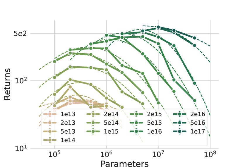
(a) IsoFLOP curves

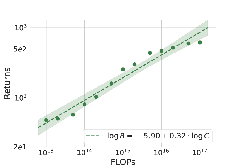
(b) Optimal return vs. FLOPs

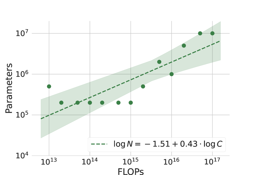
(c) Optimal parameters vs. FLOPs

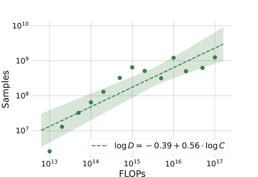
(d) Optimal samples vs. FLOPs

Figure 4: RL return scaling. We train a wide range of model sizes across several orders of magnitude of FLOP budgets and plot the average return when rolled out in the environment at the end of training (a). We then regress the return-optimal average returns (b), parameters (c), and samples (d) on their corresponding FLOP budgets. Due to computational cost, we only run 1 seed per point on the IsoFLOP profile.

7 Related work

NetHack

Work on NetHack has been quite limited so far, with early work establishing the NLE benchmark [11], evaluating symbolic vs. neural agents [10], and creating large-scale datasets based off of rule-based and human playthroughs for methods aiming to learn from demonstrations [9]. More recent work has either focused on better reward signal supervision and sample efficiency through proxy metrics and contrastive pre-training [13, 17] or leveraged dynamics models with language descriptions in order to improve sample efficiency and generalization [12]. Concurrent work also investigates the gap between neural methods and AutoAscend, but mostly focuses on leveraging an action hierarchy, improvements in architecture, and fine-tuning with RL [16].

Scaling laws

Hestness et al. [18] and Rosenfeld et al. [19] are one of the earliest works that try to characterize empirical scaling laws for deep learning. Kaplan et al. [4] and Hoffmann et al. [5] specifically focus on training compute-optimal language models, finding similar trends as presented in this paper. While in the imitation learning setting, our agents also minimize cross-entropy loss, we additionally show that the eventual performance of the agent as measured by the average return in the environment scales smoothly with the loss. Other works focus more broadly on generative modeling [20], or analyze specific use cases such as acoustic modeling [21]. Clark et al. [22] investigate scaling laws for routing networks, and Hernandez et al. [23] study scaling laws for transfer, finding the effective data transferred (the amount of extra data required to match a pre-trained model from scratch) follows a power-law in the low-data regime. More recent works have also tried to extend these scaling law results to multi-modal learning [24, 25]. Finally, Caballero et al. [26] introduces broken neural scaling laws, which allow the modeling of phenomena such as double descent as well as sharp inflection points.

Perhaps the closest work to our paper is that of Hilton et al. [15], who define a new metric called intrinsic performance to characterize scaling laws in RL across various environments. However, they don’t consider the setting where agents can learn from expert demonstrations, and they do not evaluate on NetHack, which we consider an especially interesting environment because of its extremely challenging nature.

8 Discussion

Extensions beyond NetHack.

We have shown that both in the imitation learning and reinforcement learning settings, scaling up model and data size provides a promising path to improving performance, as demonstrated in the full game of NetHack. While we do not extend our analysis beyond NetHack in this paper, we believe these results are suggestive of similar findings across many imitation learning tasks, where oftentimes model and data sizes are not carefully picked.

Leveraging human data.

One direction we did not consider in this paper is analyzing the scaling relationships when using human trajectories (e.g. from NLD-NAO [9]) instead of those from AutoAscend (NLD-AA [9]). This is because extra care must be taken to handle the lack of actions in the human dataset, requiring techniques such as BCO [27]. Investigating the scaling laws here could be especially interesting since: (1) the human dataset is more diverse, containing trajectories from many different players with varying level of skill, and (2) it contains many examples of trajectories that ascend (i.e. win the game). (1) could shed perspective on the role of scaling when the data includes many different and potentially suboptimal demonstrations, similar to Beliaev et al. [28]. (2) could provide insight into the viability of methods such as Video PreTraining (VPT) [29] since these rely heavily on being able to clone the expert data well.

RL with pretraining.

All our scaling law results on the RL side in this paper are with policies trained from scratch. However, some of the most promising neural methods for NetHack and other domains leverage a pre-trained (e.g. through imitation learning) policy that is then finetuned with RL. It would be very interesting to analyze the scaling behaviors for these kind of kickstarted policies, and see whether they scale differently than the ones trained from scratch.

Broader impacts.

While we do not see a direct path towards any negative applications, we note that scaling up could have unknown unintended consequences. As scaling results in imitation and reinforcement learning agents that are increasingly more capable and influential in our lives, it will be important to keep them aligned with human values.

9 Conclusion

In this work, we find that imitation learning loss and mean return follow clear power law trends with respect to FLOPs, as demonstrated in the challenging and unsolved game of NetHack. In addition, we find loss and mean return to be highly correlated, meaning improvements in loss predictably translate in improved performance in the environment. Using the found power laws, we forecast the compute requirements (in terms of model and data size) to train compute-optimal agents aimed at recovering the underlying expert. While our agents fall short of expert performance, we find the performance still improves dramatically, surpassing prior SOTA by 2x in all settings. We also extend our results to the reinforcement learning setting, and find similar power laws for model size and number of interactions. Our results demonstrate that scaling up model and data size is a promising path towards training increasingly capable NetHack agents. More broadly, they also call for work in the larger imitation learning and reinforcement learning community to more carefully consider and study the role of scaling laws, which could provide large improvements in many other domains.

Appendix A Parametric fit: power law derivation

In this section, we show the derivation resulting in Equation 6. We first restate Equation 4 for convenience:

$$\log\hat{L}(N,D)=\beta_{0}+\beta_{N}\log N+\beta_{D}\log D+\beta_{N^{2}}\log^{2}N+\beta_{ND}\log N\log D+\beta_{D^{2}}\log^{2}D.$$

Now, to minimize this equation with the constraint that $\mathrm{FLOPs}(N,D)=C\approx 6ND$, we use Lagrange multipliers. We first write down the Lagrangian:

$$\mathcal{L}(N,D,\lambda)=\hat{L}(N,D)-\lambda(g(N,D)-C),$$

where $g(N,D)=6ND$. Now, setting $\nabla\mathcal{L}=\bm{0}$ we get:

$$\nabla\log\hat{L}(N,D)=\lambda\nabla(6ND)\quad\text{and}\quad 6ND=C.$$

The former results in the following system of equations:

$$\frac{\partial\log\hat{L}(N,D)}{\partial N} =\lambda\frac{\partial(6ND)}{\partial N}$$

$$\frac{\partial\log\hat{L}(N,D)}{\partial D} =\lambda\frac{\partial(6ND)}{\partial D}.$$

This means that

$$\beta_{N}\frac{1}{N}+\beta_{ND}\log D\frac{1}{N}+2\beta_{N^{2}}\log N\frac{1}{N} =\lambda 6D$$

$$\beta_{D}\frac{1}{D}+\beta_{ND}\log N\frac{1}{D}+2\beta_{D^{2}}\log D\frac{1}{D} =\lambda 6N.$$

Multiplying the top equation by $N$ and the bottom one by $D$ we have that

$$\beta_{N}+\beta_{ND}\log D+2\beta_{N^{2}}\log N=\beta_{D}+\beta_{ND}\log N+2\beta_{D^{2}}\log D.$$

Recalling $C=6ND$, we solve for $N$ and $D$ in terms of $C$, giving the results listed in Equation 6.

Appendix B Full set of results

The full set of results can be found in Table 3.

	All	Human
Models	Random	Monk
Offline only
DQN-Offline [9]	0.0 $\pm$ 0.0	0.0 $\pm$ 0.0
CQL [9]	352 $\pm$ 18	366 $\pm$ 35
IQL [9]	171 $\pm$ 6	267 $\pm$ 28
BC (CDGPT5) [9, 10]	554 $\pm$ 45	1059 $\pm$ 159
BC (Transformer) [16]	1318 $\pm$ 38	-
Scaled-BC (ours)	2740 $\pm$ -	5218 $\pm$ -
Offline + Online
Kickstarting + BC [9]	962 $\pm$ 50	2090 $\pm$ 123
APPO + BC [9]	1282 $\pm$ 87	2809 $\pm$ 103
APPO + BC [16]	1551 $\pm$ 73	-
LDD∗ [12]	-	2100 $\pm$ -

Table 3: Forecasting results (full). 2(b) with added standard errors. Results from Hambro et al. [9] use 10 seeds, those from Piterbarg et al. [16] use 6 seeds, while ours are 1 seed due to computational cost. ^∗Exact scores not reported in original work. Scores from Hambro et al. [9] were adjusted to account for an error in their original evaluation code.

Appendix C Additional figures

We show the full set of IsoFLOP curves for all settings in Figure 5.

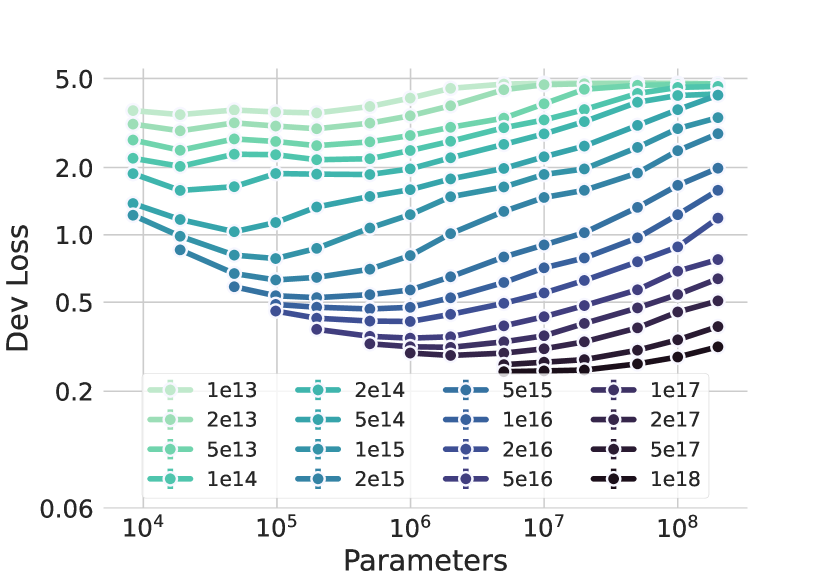
(a) BC Loss IsoFLOP curves

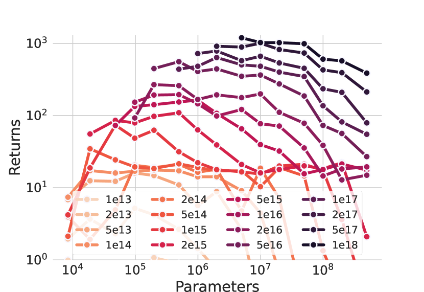
(b) BC Return IsoFLOP curves

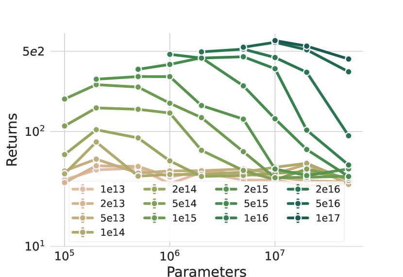
(c) RL Return IsoFLOP curves

Figure 5: Full isoFLOP curves. (a) is similar to 1(a) but including the full set of points. (b) is similar to 2(a) but including the full set of points. (c) is similar to 4(a) but including the full set of points.

Appendix D Architecture details

We use two main architectures for all our experiments, one for the BC experiments and another for the RL experiments.

BC architecture.

The NLD-AA dataset [9] is comprised of ttyrec-formatted trajectories, which are $24\times 80$ ASCII character and color grids (one for each) along with the cursor position. To encode these, we modify the architecture used in Hambro et al. [9], resulting in the following:

• Dungeon encoder. This component encodes the main observation in the game, which is a $21\times 80$ grid per time step. Note the top row and bottom two rows are cut off as those are fed into the message and bottom line statistics encoder, respectively. We embed each character and color in an embedding lookup table, after which we concatenate them and put them in their respective positions in the grid. We then feed this embedded grid into a ResNet, which consists of 2 identical modules, each using 1 convolutional layer followed by a max pooling layer and 2 residual blocks (of 2 convolutional layers each), for a total of 10 convolutional layers, closely following the setup in Espeholt et al. [14].

• Message encoder. The message encoder takes the top row of the grid, converts all ASCII characters into a one-hot vector, and concatenates these, resulting in a $80\times 256=20,480$ dimensional vector representing the message. This vector is then fed into a 2-layer MLP, resulting in the message representation.

• Bottom line statistics. To encode the bottom line statistics, we flatten the bottom two rows of the grid and create a “character-normalized" (subtract 32 and divide by 96) and “digits-normalized" (subtract 47 and divide by 10, mask out ASCII characters smaller than 45 or larger than 58) input representation, which we then stack, resulting in a $160\times 2$ dimensional input. This closely follows the Sample Factory model used in Hambro et al. [9].

After the components above are encoded, we concatenate all of them together. Additionally, we also concatenate the previous frame’s action representation (coming from an embedding lookup table), and a crop representation (a $9\times 9$ crop around the player, processed by a 5-layer CNN). We then feed this combined representation into a 2-layer MLP, after which a single layer LSTM processes the representation further. Finally, we have two linear heads on top of the LSTM, one for the policy and one for the value (not used for BC).

RL architecture.

We modify the architecture from Küttler et al. [11] to also include a 5-layer 1-dimensional CNN that processes the message, as well as another 5-layer 2-dimensional CNN that processes a $9\times 9$ crop of the dungeon grid around the player.

Appendix E FLOP and parameter counting

As mentioned in the main text, we only count FLOPs and parameters for the parts of the model being scaled. For all our BC and RL experiments, we only scale the following parts of the model and keep the rest fixed:

• The hidden size of the two-layer MLP right before the LSTM.

• The hidden size of the LSTM.

• The input size of the two linear layers for the actor and critic respectively (i.e. the policy and value heads).

Similar to prior work [4, 5], we found $6ND$ to be a good approximation for the number of FLOPs used based on model size $N$ and number of samples $D$. This is because we found there to be about $2ND$ FLOPs in the forward pass, and we assume the backward pass takes about the twice the number of FLOPs from the forward pass.

For the RL experiments, there is a slight change in the way we count FLOPs, which is that we count every forward pass number of FLOPs from the learner twice, since there is a corresponding forward pass from an actor. Hence, for RL our formula becomes $8ND$.

Appendix F Training details

We use Adam [30] as our optimizer for all BC experiments. For RL, we use RMSprop. Please find all hyperparameters for both settings in Table 4, all of which were manually tuned or taken from prior work. All experiments were run on NVIDIA V100 32GB or A100 40GB GPUs, and took up to 4 days to run, depending on the FLOP budget. The one exception to this is our forecasted BC model which consisted of 30M parameters and was run on 115B samples. This took approximately 11 days, and was partially run on a A100 GPU, and continued on a V100 GPU.

The NLD-AA dataset [9] is released under the NetHack General Public License and can be found at https://github.com/dungeonsdatasubmission/dungeonsdata-neurips2022.

Hyperparameters	Value
Learning rate	0.0001
Batch size	$128\times 8$ (8 GPUs)
Unroll length	80
Ttyrec workers	30

(a) BC hyperparameters

Hyperparameter	Value
Learning rate	0.0002
Learner batch size	32
Unroll length	80
Entropy cost	0.001
Baseline cost	0.5
Maximum episode steps	5000
Reward normalization	yes
Reward clipping	none
Number of actors	90
Discount factor	0.99

(b) RL hyperparameters

Table 4: Hyperparameters for all experiments. We list the hyperparameters for all our BC experiments (a) as well as the ones for our RL experiments (b).

Appendix G Delta method derivation

Following standard linear regression assumptions, we have that $\sqrt{n}(\bm{\hat{\beta}}-\bm{\beta})\xrightarrow{D}\mathcal{N}(0,\Sigma)$, where $\bm{\hat{\beta}}$ is a vector containing all regression coefficients, i.e.

$$\bm{\hat{\beta}}=\langle\hat{\beta}_{0},\hat{\beta}_{N},\hat{\beta}_{D},\hat{\beta}_{N^{2}},\hat{\beta}_{ND},\hat{\beta}_{D^{2}}\rangle$$

We also rewrite $\alpha$ from Equation 6 more explicitly as a function $h$:

$$\alpha=h(\bm{\hat{\beta}})=\frac{2\beta_{D^{2}}-\beta_{ND}}{2\beta_{D^{2}}-2\beta_{ND}+2\beta_{N^{2}}}$$

Approximating $h(\bm{\hat{\beta}})$ with a first-order Taylor expansion around $\bm{\beta}$ we get:

$$h(\bm{\hat{\beta}})\approx h(\bm{\beta})+\nabla h(\bm{\beta})^{T}\cdot(\bm{\hat{\beta}}-\bm{\beta})$$

Computing the variance of $h(\bm{\hat{\beta}})$ then gives:

$$\mathrm{Var}[h(\bm{\hat{\beta}})] =\mathrm{Var}[h(\bm{\beta})+\nabla h(\bm{\beta})^{T}\cdot(\hat{\bm{\beta}}-\bm{\beta})]$$

$$=\mathrm{Var}[h(\bm{\beta})+\nabla h(\bm{\beta})^{T}\cdot\hat{\bm{\beta}}-\nabla h(\bm{\beta})^{T}\cdot\bm{\beta}]$$

$$=\mathrm{Var}[\nabla h(\bm{\beta})^{T}\cdot\bm{\hat{\beta}}]$$

$$=\nabla h(\bm{\beta})^{T}\cdot\mathrm{Cov}(\bm{\hat{\beta}})\cdot\nabla h(\bm{\beta})$$

$$=\nabla h(\bm{\beta})^{T}\frac{\Sigma}{n}\nabla h(\bm{\beta})$$

Now the Standard Error (SE) can be found as

$$\mathrm{SE}=\sqrt{\nabla h(\bm{\beta})^{T}\frac{\Sigma}{n}\nabla h(\bm{\beta})}.$$

Finally, we approximate the SE above by using $\nabla h(\bm{\hat{\beta}})$ instead of $\nabla h(\bm{\beta})$, giving the following confidence interval:

$$\mathrm{CI}=h(\bm{\hat{\beta}})\pm 1.96\cdot\mathrm{SE}.$$

Appendix H Cross-validation

To measure forecasting performance of all power law regressions done in the paper, we leverage a rolling time series cross-validation. Specifically, for every regression, we initially take the first 6 points (corresponding to the first 6 FLOP budgets) to be our training set to fit the regression, and then compute the RMSE on the 7th point. Then, we include the 7th point in our training set and evaluate on the 8th point. This process keeps going until all but the last point is included, after which we average all resulting RMSEs. Note that this process ensures we always evaluate on future FLOP budgets. Results can be found in Table 5.

To provide further insight into our time-series-based cross-validation results, we also visualize the progression of the $\beta_{0}$ and $\beta_{1}$ parameters in Figure 6, Figure 7, Figure 8, and Figure 9.

Regressions	Dev RMSE
Loss minima vs. FLOPs ( 1(b))	$7.7e^{-2}$
Loss-optimal parameters vs. FLOPs ( 1(c))	$4.3e^{5}$
Loss-optimal samples vs. FLOPs ( 1(d))	$3.8e^{9}$
BC maximal returns vs. FLOPs ( 2(b))	$3.9e^{2}$
BC return-optimal parameters vs. FLOPs ( 2(c))	$1.6e^{6}$
BC return-optimal samples vs. FLOPs ( 2(d))	$1.7e^{10}$
BC returns vs. loss minima ( 3(a))	$1.2e^{2}$
BC returns vs. loss-optimal parameters ( 3(b))	$3.8e^{2}$
BC returns vs. loss-optimal samples ( 3(c))	$2.0e^{2}$
RL maximal returns vs. FLOPs ( 4(b))	$1.4e^{2}$
RL return-optimal parameters vs. FLOPs ( 4(c))	$2.9e^{6}$
RL return-optimal samples vs. FLOPs ( 4(d))	$1.6e^{9}$

Table 5: Cross-validation RMSEs. We use a time series rolling cross-validation to compute the average Root Mean Squared Error (RMSE) for all regressions done in the paper.

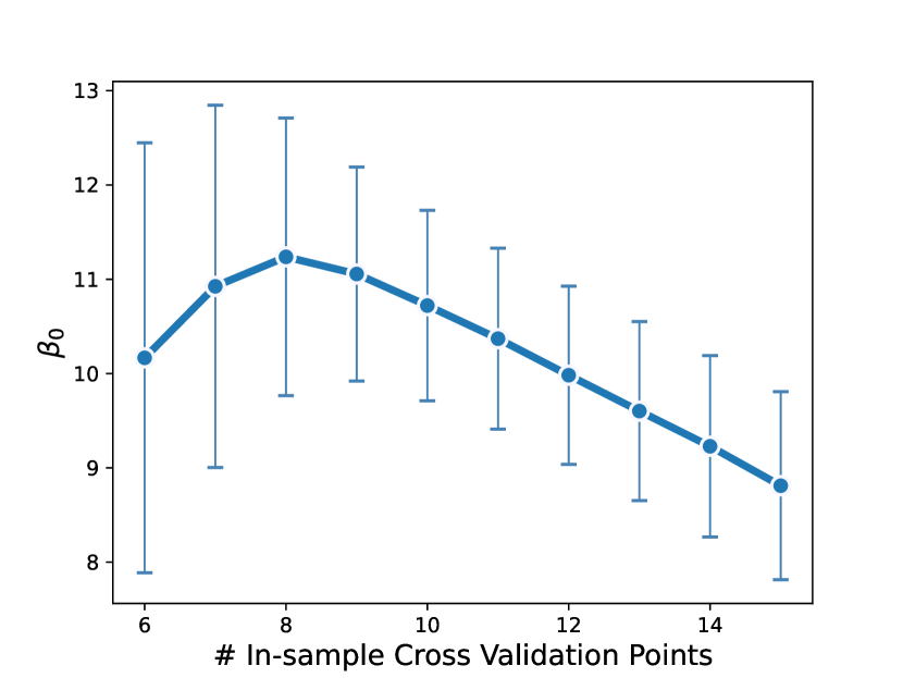
(a) Loss vs. FLOPs $\beta_{0}$

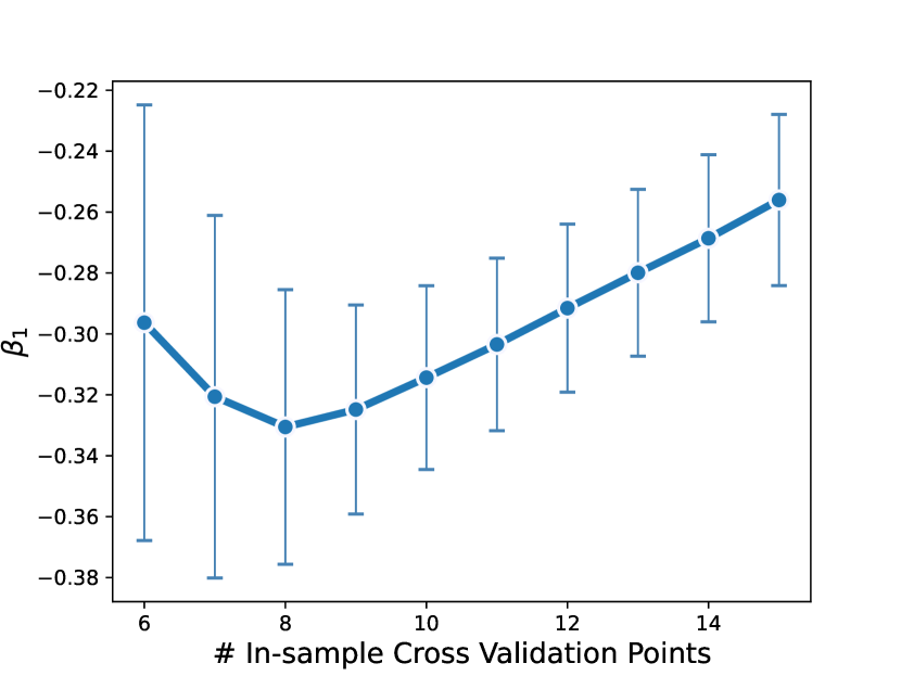
(b) Loss vs. FLOPs $\beta_{1}$

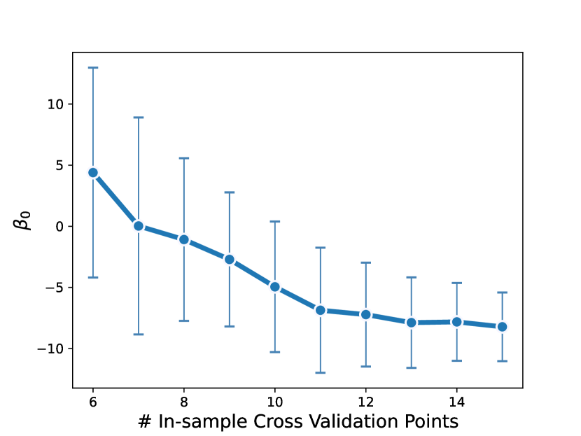
(c) Optimal parameters vs. FLOPs $\beta_{0}$

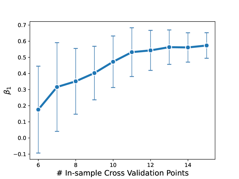
(d) Optimal parameters vs. FLOPs $\beta_{1}$

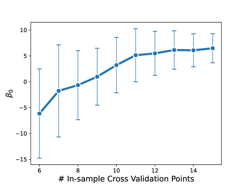
(e) Optimal samples vs. FLOPs $\beta_{0}$

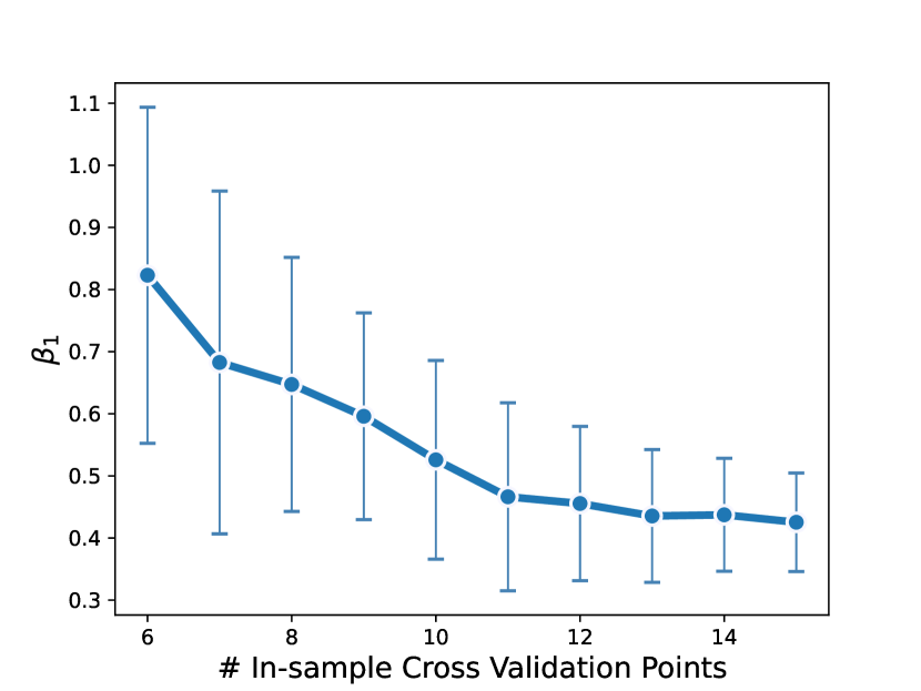
(f) Optimal samples vs. FLOPs $\beta_{1}$

Figure 6: BC loss cross validation progression. We leverage a time-series-based rolling cross-validation going from early to later FLOP budgets, and visualize the progression of the $\beta_{0}$ and $\beta_{1}$ coefficients.

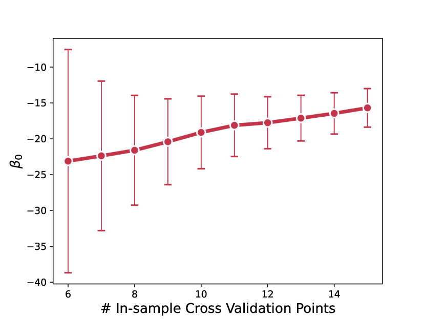
(a) Return vs. FLOPs $\beta_{0}$

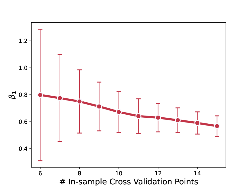
(b) Return vs. FLOPs $\beta_{1}$

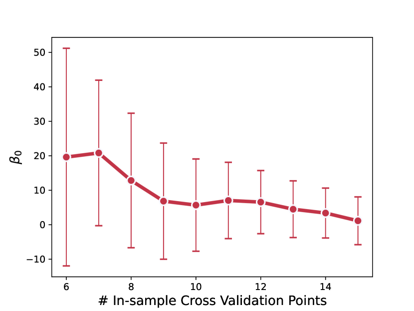
(c) Parameters vs. FLOPs $\beta_{0}$

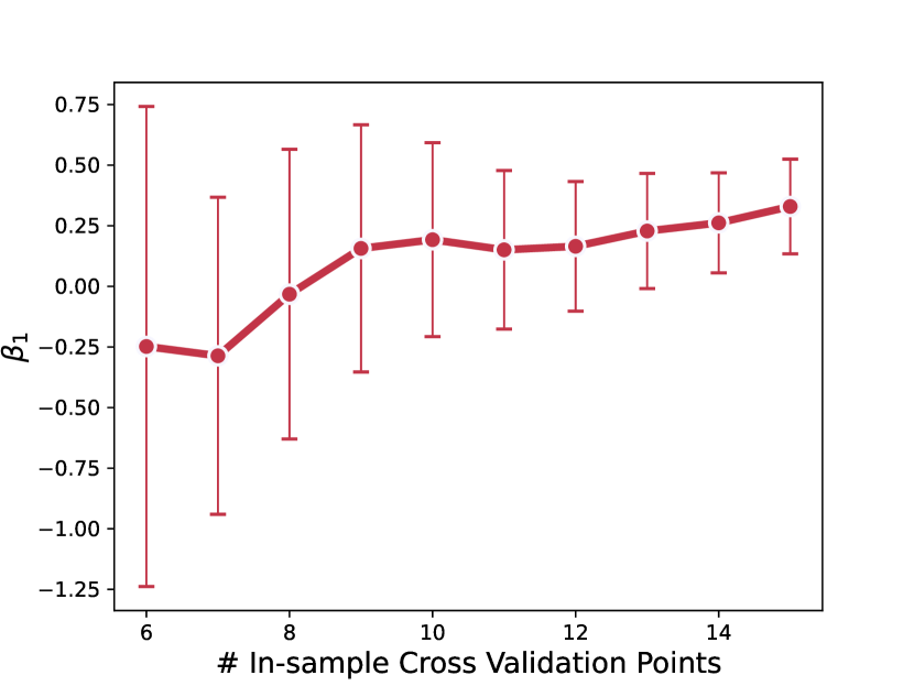
(d) Parameters vs. FLOPs $\beta_{1}$

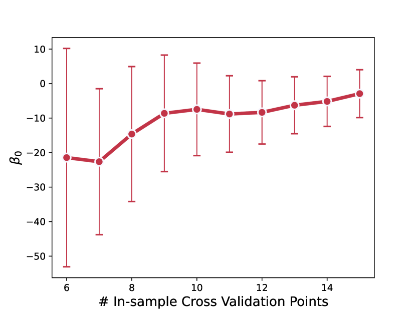
(e) Samples vs. FLOPs $\beta_{0}$

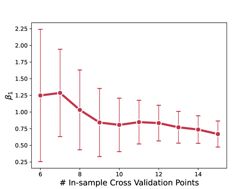
(f) Samples vs. FLOPs $\beta_{1}$

Figure 7: BC return cross validation progression. We leverage a time-series-based rolling cross-validation going from early to later FLOP budgets, and visualize the progression of the $\beta_{0}$ and $\beta_{1}$ coefficients.

(a) Return vs. optimal 1 / loss $\beta_{0}$

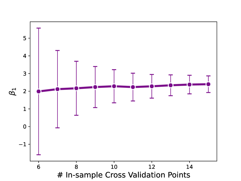
(b) Return vs. optimal 1 / loss $\beta_{1}$

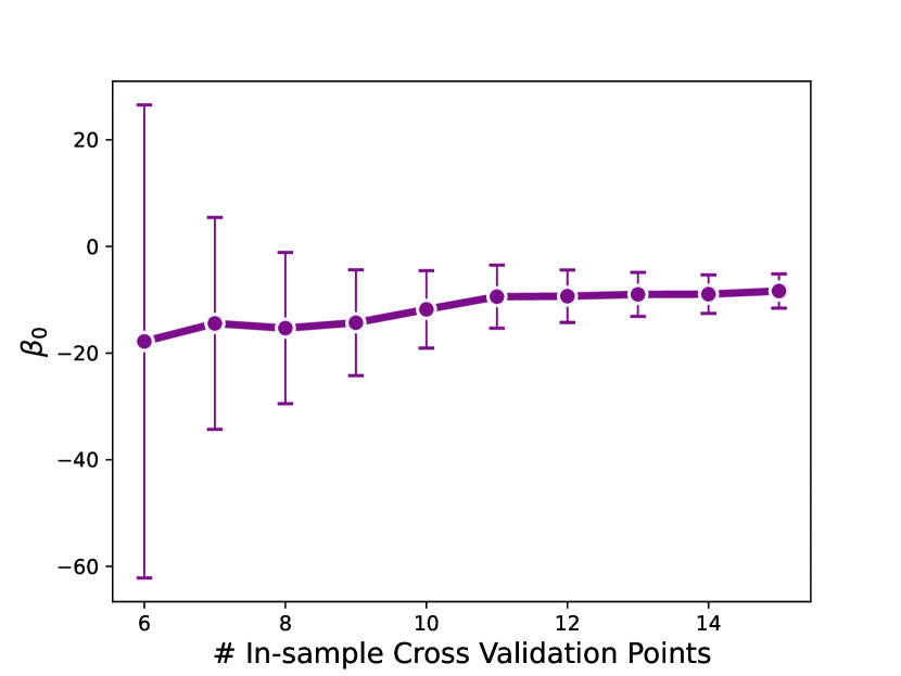
(c) Return vs. loss-optimal parameters $\beta_{0}$

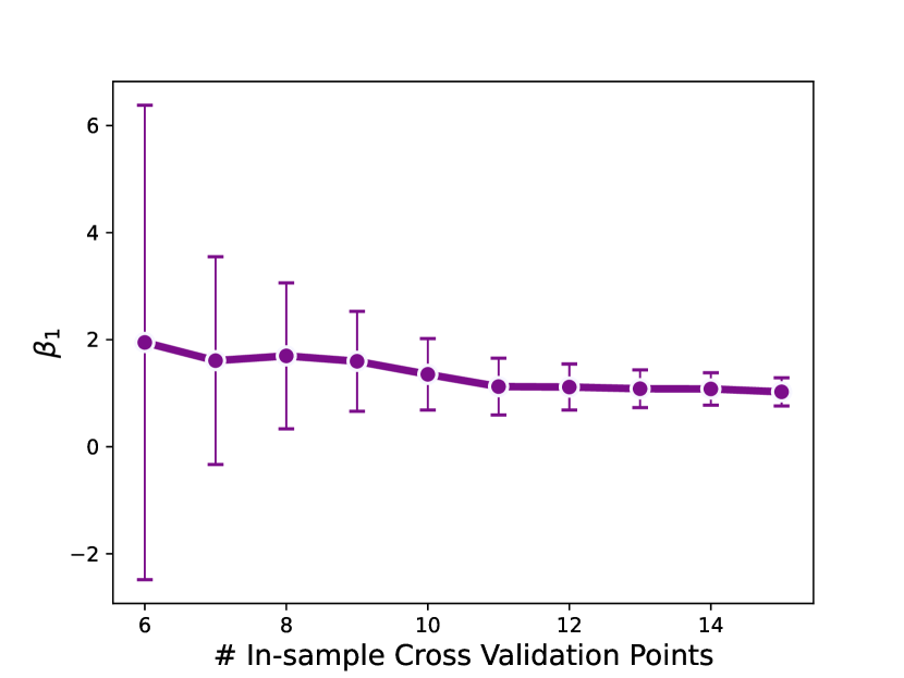
(d) Return vs. loss-optimal parameters $\beta_{1}$

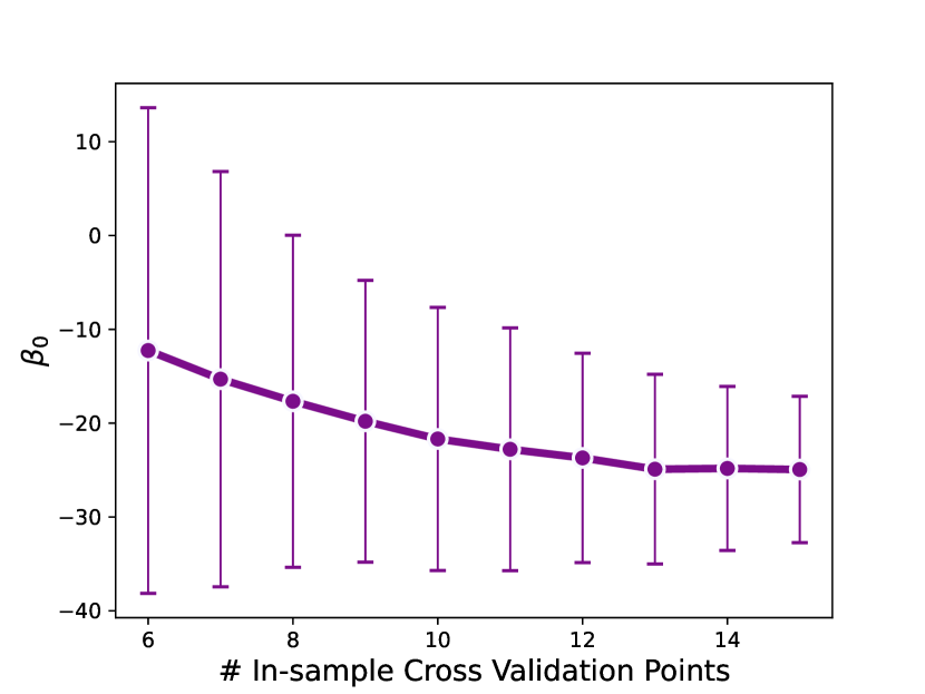
(e) Return vs. loss-optimal samples $\beta_{0}$

(f) Return vs. loss-optimal samples $\beta_{1}$

Figure 8: BC return-loss relation cross validation progression. We leverage a time-series-based rolling cross-validation going from early to later FLOP budgets, and visualize the progression of the $\beta_{0}$ and $\beta_{1}$ coefficients.

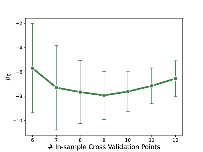
(a) Return vs. FLOPs $\beta_{0}$

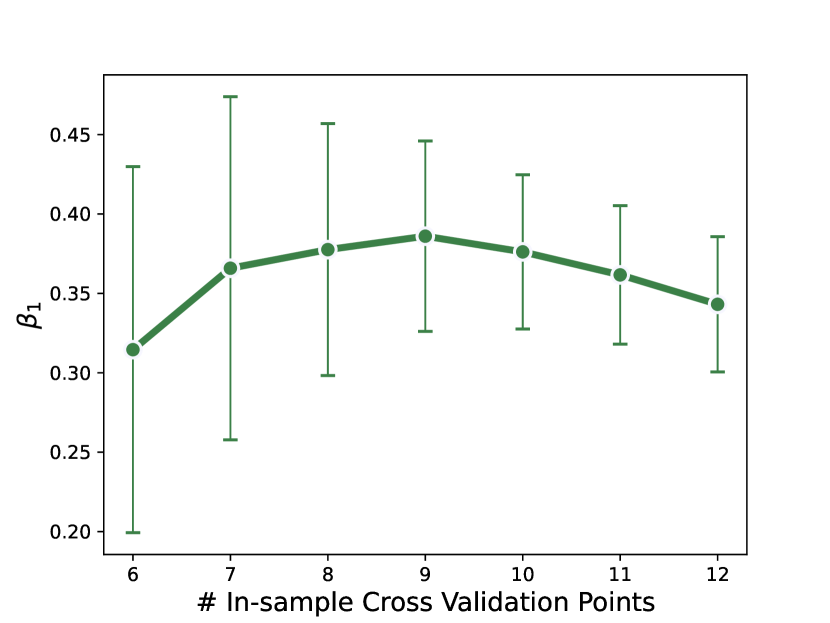
(b) Return vs. FLOPs $\beta_{1}$

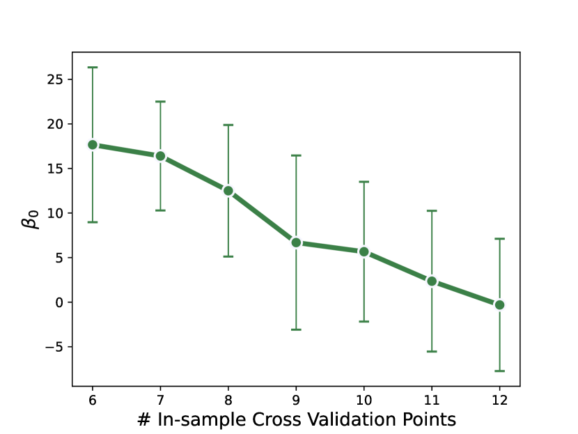
(c) Optimal parameters vs. FLOPs $\beta_{0}$

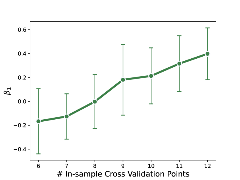
(d) Optimal parameters vs. FLOPs $\beta_{1}$

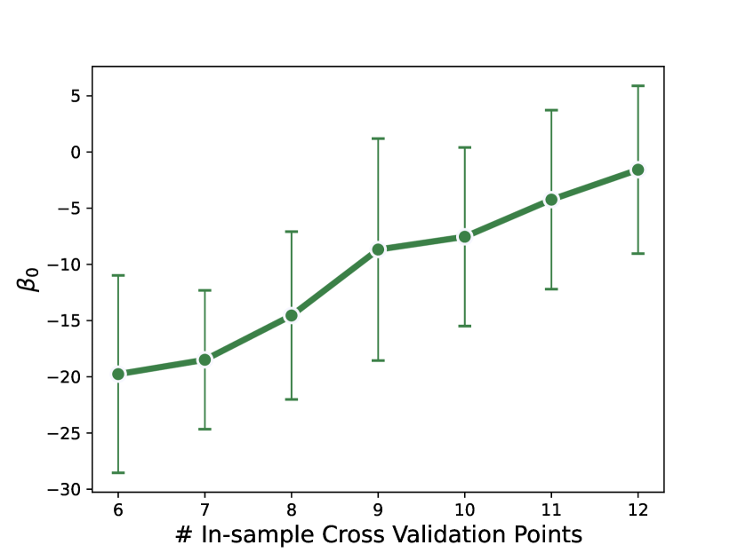
(e) Optimal samples vs. FLOPs $\beta_{0}$

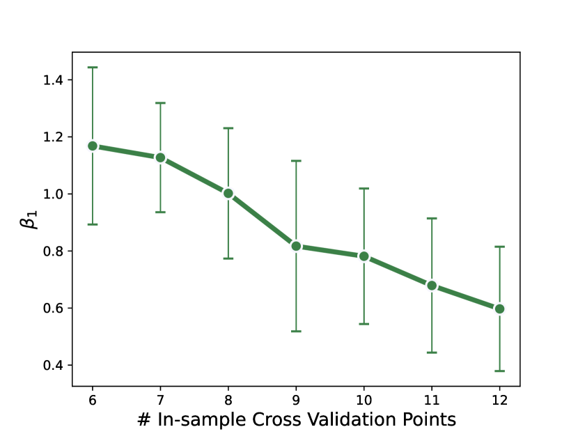
(f) Optimal samples vs. FLOPs $\beta_{1}$

Figure 9: RL return cross validation progression. We leverage a time-series-based rolling cross-validation going from early to later FLOP budgets, and visualize the progression of the $\beta_{0}$ and $\beta_{1}$ coefficients.

References

- Wen et al. [2020] Chuan Wen, Jierui Lin, Trevor Darrell, Dinesh Jayaraman, and Yang Gao. Fighting copycat agents in behavioral cloning from observation histories. Advances in Neural Information Processing Systems, 33:2564–2575, 2020.
- De Haan et al. [2019] Pim De Haan, Dinesh Jayaraman, and Sergey Levine. Causal confusion in imitation learning. Advances in Neural Information Processing Systems, 32, 2019.
- Jacob et al. [2022] Athul Paul Jacob, David J Wu, Gabriele Farina, Adam Lerer, Hengyuan Hu, Anton Bakhtin, Jacob Andreas, and Noam Brown. Modeling strong and human-like gameplay with kl-regularized search. In International Conference on Machine Learning, pages 9695–9728. PMLR, 2022.
- Kaplan et al. [2020] Jared Kaplan, Sam McCandlish, Tom Henighan, Tom B Brown, Benjamin Chess, Rewon Child, Scott Gray, Alec Radford, Jeffrey Wu, and Dario Amodei. Scaling laws for neural language models. arXiv preprint arXiv:2001.08361, 2020.
- Hoffmann et al. [2022] Jordan Hoffmann, Sebastian Borgeaud, Arthur Mensch, Elena Buchatskaya, Trevor Cai, Eliza Rutherford, Diego de Las Casas, Lisa Anne Hendricks, Johannes Welbl, Aidan Clark, et al. Training compute-optimal large language models. arXiv preprint arXiv:2203.15556, 2022.
- Silver et al. [2016] David Silver, Aja Huang, Chris J. Maddison, Arthur Guez, Laurent Sifre, George van den Driessche, Julian Schrittwieser, Ioannis Antonoglou, Veda Panneershelvam, Marc Lanctot, Sander Dieleman, Dominik Grewe, John Nham, Nal Kalchbrenner, Ilya Sutskever, Timothy Lillicrap, Madeleine Leach, Koray Kavukcuoglu, Thore Graepel, and Demis Hassabis. Mastering the game of go with deep neural networks and tree search. Nature, 529(7587):484–489, Jan 2016. ISSN 1476-4687. doi: 10.1038/nature16961. URL https://doi.org/10.1038/nature16961.
- Ahn et al. [2022] Michael Ahn, Anthony Brohan, Noah Brown, Yevgen Chebotar, Omar Cortes, Byron David, Chelsea Finn, Keerthana Gopalakrishnan, Karol Hausman, Alex Herzog, et al. Do as i can, not as i say: Grounding language in robotic affordances. arXiv preprint arXiv:2204.01691, 2022.
- Ecoffet et al. [2021] Adrien Ecoffet, Joost Huizinga, Joel Lehman, Kenneth O. Stanley, and Jeff Clune. First return, then explore. Nature, 590(7847):580–586, Feb 2021. ISSN 1476-4687. doi: 10.1038/s41586-020-03157-9. URL https://doi.org/10.1038/s41586-020-03157-9.
- Hambro et al. [2022a] Eric Hambro, Roberta Raileanu, Danielle Rothermel, Vegard Mella, Tim Rocktäschel, Heinrich Küttler, and Naila Murray. Dungeons and data: A large-scale nethack dataset. In S. Koyejo, S. Mohamed, A. Agarwal, D. Belgrave, K. Cho, and A. Oh, editors, Advances in Neural Information Processing Systems, volume 35, pages 24864–24878. Curran Associates, Inc., 2022a. URL https://proceedings.neurips.cc/paper_files/paper/2022/file/9d9258fd703057246cb341e615426e2d-Paper-Datasets_and_Benchmarks.pdf.
- Hambro et al. [2022b] Eric Hambro, Sharada Mohanty, Dmitrii Babaev, Minwoo Byeon, Dipam Chakraborty, Edward Grefenstette, Minqi Jiang, Jo Daejin, Anssi Kanervisto, Jongmin Kim, et al. Insights from the neurips 2021 nethack challenge. In NeurIPS 2021 Competitions and Demonstrations Track, pages 41–52. PMLR, 2022b.
- Küttler et al. [2020] Heinrich Küttler, Nantas Nardelli, Alexander Miller, Roberta Raileanu, Marco Selvatici, Edward Grefenstette, and Tim Rocktäschel. The nethack learning environment. Advances in Neural Information Processing Systems, 33:7671–7684, 2020.
- Mu et al. [2022] Jesse Mu, Victor Zhong, Roberta Raileanu, Minqi Jiang, Noah Goodman, Tim Rocktäschel, and Edward Grefenstette. Improving intrinsic exploration with language abstractions. In S. Koyejo, S. Mohamed, A. Agarwal, D. Belgrave, K. Cho, and A. Oh, editors, Advances in Neural Information Processing Systems, volume 35, pages 33947–33960. Curran Associates, Inc., 2022. URL https://proceedings.neurips.cc/paper_files/paper/2022/file/db8cf88ced2536017980998929ee0fdf-Paper-Conference.pdf.
- Mazoure et al. [2023] Bogdan Mazoure, Jake Bruce, Doina Precup, Rob Fergus, and Ankit Anand. Accelerating exploration and representation learning with offline pre-training. arXiv preprint arXiv:2304.00046, 2023.
- Espeholt et al. [2018] Lasse Espeholt, Hubert Soyer, Remi Munos, Karen Simonyan, Vlad Mnih, Tom Ward, Yotam Doron, Vlad Firoiu, Tim Harley, Iain Dunning, et al. Impala: Scalable distributed deep-rl with importance weighted actor-learner architectures. In International conference on machine learning, pages 1407–1416. PMLR, 2018.
- Hilton et al. [2023] Jacob Hilton, Jie Tang, and John Schulman. Scaling laws for single-agent reinforcement learning. arXiv preprint arXiv:2301.13442, 2023.
- Piterbarg et al. [2023] Ulyana Piterbarg, Lerrel Pinto, and Rob Fergus. Nethack is hard to hack. arXiv preprint arXiv:2305.19240, 2023.
- Bruce et al. [2023] Jake Bruce, Ankit Anand, Bogdan Mazoure, and Rob Fergus. Learning about progress from experts. In International Conference on Learning Representations, 2023.
- Hestness et al. [2017] Joel Hestness, Sharan Narang, Newsha Ardalani, Gregory Diamos, Heewoo Jun, Hassan Kianinejad, Md Patwary, Mostofa Ali, Yang Yang, and Yanqi Zhou. Deep learning scaling is predictable, empirically. arXiv preprint arXiv:1712.00409, 2017.
- Rosenfeld et al. [2019] Jonathan S Rosenfeld, Amir Rosenfeld, Yonatan Belinkov, and Nir Shavit. A constructive prediction of the generalization error across scales. arXiv preprint arXiv:1909.12673, 2019.
- Henighan et al. [2020] Tom Henighan, Jared Kaplan, Mor Katz, Mark Chen, Christopher Hesse, Jacob Jackson, Heewoo Jun, Tom B Brown, Prafulla Dhariwal, Scott Gray, et al. Scaling laws for autoregressive generative modeling. arXiv preprint arXiv:2010.14701, 2020.
- Droppo and Elibol [2021] Jasha Droppo and Oguz Elibol. Scaling laws for acoustic models. arXiv preprint arXiv:2106.09488, 2021.
- Clark et al. [2022] Aidan Clark, Diego de Las Casas, Aurelia Guy, Arthur Mensch, Michela Paganini, Jordan Hoffmann, Bogdan Damoc, Blake A. Hechtman, Trevor Cai, Sebastian Borgeaud, George van den Driessche, Eliza Rutherford, T. W. Hennigan, Matthew G. Johnson, Katie Millican, Albin Cassirer, Chris Jones, Elena Buchatskaya, David Budden, L. Sifre, Simon Osindero, Oriol Vinyals, Jack W. Rae, Erich Elsen, Koray Kavukcuoglu, and Karen Simonyan. Unified scaling laws for routed language models. In International Conference on Machine Learning, 2022.
- Hernandez et al. [2021] Danny Hernandez, Jared Kaplan, Tom Henighan, and Sam McCandlish. Scaling laws for transfer. arXiv preprint arXiv:2102.01293, 2021.
- Cherti et al. [2022] Mehdi Cherti, Romain Beaumont, Ross Wightman, Mitchell Wortsman, Gabriel Ilharco, Cade Gordon, Christoph Schuhmann, Ludwig Schmidt, and Jenia Jitsev. Reproducible scaling laws for contrastive language-image learning. arXiv preprint arXiv:2212.07143, 2022.
- Aghajanyan et al. [2023] Armen Aghajanyan, Lili Yu, Alexis Conneau, Wei-Ning Hsu, Karen Hambardzumyan, Susan Zhang, Stephen Roller, Naman Goyal, Omer Levy, and Luke Zettlemoyer. Scaling laws for generative mixed-modal language models. arXiv preprint arXiv:2301.03728, 2023.
- Caballero et al. [2022] Ethan Caballero, Kshitij Gupta, Irina Rish, and David Krueger. Broken neural scaling laws. arXiv preprint arXiv:2210.14891, 2022.
- Torabi et al. [2018] Faraz Torabi, Garrett Warnell, and Peter Stone. Behavioral cloning from observation. In Proceedings of the 27th International Joint Conference on Artificial Intelligence, pages 4950–4957, 2018.
- Beliaev et al. [2022] Mark Beliaev, Andy Shih, Stefano Ermon, Dorsa Sadigh, and Ramtin Pedarsani. Imitation learning by estimating expertise of demonstrators. In International Conference on Machine Learning, pages 1732–1748. PMLR, 2022.
- Baker et al. [2022] Bowen Baker, Ilge Akkaya, Peter Zhokov, Joost Huizinga, Jie Tang, Adrien Ecoffet, Brandon Houghton, Raul Sampedro, and Jeff Clune. Video pretraining (vpt): Learning to act by watching unlabeled online videos. Advances in Neural Information Processing Systems, 35:24639–24654, 2022.
- Kingma and Ba [2014] Diederik P Kingma and Jimmy Ba. Adam: A method for stochastic optimization. arXiv preprint arXiv:1412.6980, 2014.