The stellar thermal wind as a consequence of oblateness

Abstract

In many rotating fluids, the lowest-order force balance is between gravity, pressure, and rotational acceleration (‘GPR’ balance). Terrestrial GPR balance takes the form of geostrophy and hydrostasy, which together yield the terrestrial thermal wind equation. By contrast, stellar GPR balance is an oblateness equation, which determines the departures of the thermal variables from spherical symmetry; its curl yields the ‘stellar thermal wind equation.’ In this sense, the stellar thermal wind should be viewed not as a consequence of geostrophy, but of baroclinicity in the oblateness. Here we treat the full stellar oblateness, including the thermal wind, using pressure coordinates. We derive the generalised stellar thermal wind equation and identify the parameter regime for which it holds. In the case of the Sun, not considering the full oblateness has resulted in conflicting calculations of the theoretical aspherical temperature anomaly. We provide new calculation here and find that the baroclinic anomaly is $\sim$3–60 times smaller than the barotropic anomaly. Thus, the anomaly from the thermal wind may not be measurable helioseismically; but if measurement were possible, this would potentially yield a new way to bracket the depth of the solar tachocline.

1 The Terrestrial Thermal Wind

In many rotating fluids, the lowest-order force balance is between gravity, pressure, and rotational acceleration (hereafter ‘GPR’ balance). In the Earth’s atmosphere and oceans, GPR balance takes the form of hydrostasy in the vertical (i.e., radial) direction (pressure balancing gravity) and geostrophy in the horizontal (i.e., latitudinal and longitudinal) directions (pressure balancing the Coriolis force). When combined, hydrostasy and geostrophy yield the terrestrial thermal wind equations. Before briefly describing these equations, we emphasize the special properties of Earth that make it possible to neglect the fictitious centrifugal force (and simultaneously the Earth’s oblateness) from the equations.

First and foremost, oblateness itself is quite small: for example, if we define an object’s geometric oblateness$f\equiv(R_{\rm{eq}}-R_{\rm{pol}})/R_{\rm{eq}}$ (where $R_{\rm{eq}}$ is the object’s equatorial radius and $R_{\rm{pol}}$ its polar radius), then $f_{\oplus}=3.35\times 10^{-3}$ (e.g., Chao 2006). Second, the shape of the oblateness is such that the Earth’s surface is everywhere almost orthogonal to the effective gravity $\bm{g}_{\rm{eff}}$ (we define $\bm{g}_{\rm{eff}}\equiv\bm{g}_{\oplus}+\lambda\Omega_{\oplus}^{2}\hat{\bm{e}}_{\lambda}$, where $\bm{g}_{\oplus}$ is Earth’s gravitational acceleration, $\lambda$ the cylindrical moment arm, $\Omega_{\oplus}$ Earth’s rotation rate, and $\hat{\bm{e}}$ denotes a unit vector). The fluid flows can thus be described using spherical coordinates $r,\theta,$ and $\phi$ (radius, colatitude, and longitude, respectively) and $\bm{g}_{\rm{eff}}$ becomes purely radial. Ignoring the fictitious centrifugal force then leads to a slight error (dependent on latitude) in the magnitude of $\bm{g}_{\rm{eff}}$ and ignoring the oblateness leads to geometric errors in, for example, the operators $\partial/\partial r$ and $\partial/\partial\theta$. Both these errors are of order $f_{\oplus}$ and do not have any significant dynamical effects.

One more important property is the thinness of Earth’s oceans and atmosphere. The typical aspect ratio $\alpha$ of large-scale flow (ratio of the flow’s vertical length-scale to its horizontal length-scale) is thus quite small. Coriolis forces from the horizontal component of angular velocity can then be neglected to order $\alpha$ (e.g., Pedlosky 1987, p. 48) and the momentum equation for steady flows splits into a hydrostatic vertical component and a geostrophic horizontal component:

$$\frac{\partial P}{\partial r} =-\rho g_{\oplus},$$ (1)

$$\text{and}\ \ \ \ \ u_{\phi} =\frac{1}{2\Omega_{\oplus}\cos\theta}\frac{1}{\rho R_{\oplus}}\left(\frac{\partial P}{\partial\theta}\right)_{r},$$ (2)

where we have defined the pressure ($P$), density ($\rho$), fluid velocity ($\bm{u}$), $g_{\oplus}\equiv|\bm{g}_{\rm{eff}}|$ (presumed constant), and the radius of Earth ($R_{\oplus}$).

Throughout this work we explicitly distinguish between colatitudinal derivatives along spherical surfaces (constant $r$, denoted by $(\partial/\partial\theta)_{r}$) and isobaric surfaces (constant $P$, denoted by $(\partial/\partial\theta)_{P}$). Given a pressure field $P$, equation (2) defines the geostrophic wind $u_{\phi}$. Differentiating equation (2) by $r$ and using equation (1) yields the terrestrial thermal wind equation:

$$\frac{\partial u_{\phi}}{\partial r} =\frac{1}{2\Omega_{\oplus}\cos\theta}\frac{1}{\rho^{2}}(\nabla P\times\nabla\rho)_{\phi}$$

$$=-\frac{1}{2\Omega_{\oplus}\cos\theta}\frac{g_{\oplus}}{\rho}\frac{1}{R_{\oplus}}\left(\frac{\partial\rho}{\partial\theta}\right)_{P}.$$ (3)

Equation (1) defines the terrestrial thermal wind $\partial u_{\phi}/\partial r$—the radial gradient of the geostrophic wind (e.g., Vallis 2017, p. 91).

Equations (1) and (2) also require a small Rossby number ${\rm{Ro}}$ (ratio of advective force to Coriolis force) and a small Ekman number ${\rm{Ek}}$ (ratio of viscous force to Coriolis force). The order to which equation (1) holds is thus set by the largest of $f_{\oplus}$, $\alpha$, ${\rm{Ro}}$, and ${\rm{Ek}}$. For large-scale atmospheric winds, the rough ordering is $1\gtrsim{\rm{Ro}}\gtrsim\alpha\gtrsim f_{\oplus}\gtrsim\gg{\rm{Ek}}$ (e.g., Pedlosky 1987).

2 The Stellar Thermal Wind

In this section, we consider an axisymmetric, differentially rotating star. GPR balance might be expected to yield stellar analogs of the geostrophic and thermal winds. However, the flows in a star do not in general have small aspect ratio, nor are they confined to a surface perpendicular to $\bm{g}_{\rm{eff}}$. It is thus not justifiable to ignore the fictitious centrifugal force, use spherical coordinates while ignoring the oblateness, and assume hydrostatic and geostrophic balance. Nevertheless, this ‘terrestrial approach’ (e.g., Thompson et al. 2003; Brun et al. 2010; Aurnou & Aubert 2011; Matilsky et al. 2020) is often used to yield a stellar thermal wind equation:

$$2\Omega_{0}\frac{\partial\Omega_{*}}{\partial z}=\frac{\overline{g}}{r^{2}\sin\theta\overline{c_{P}}}\left(\frac{\partial S^{\prime}}{\partial\theta}\right)_{r}.$$ (4)

Here, $\Omega_{*}=\Omega_{*}(\lambda,z)$ is the star’s (differential) rotation rate, $\Omega_{0}$ some typical (constant) ‘reference’ value of $\Omega_{*}$, $c_{P}$ the specific heat at constant pressure, $S$ the specific entropy, and $z=r\cos\theta$ the axial coordinate. An overbar denotes a spherically-symmetric mean and a prime the deviation from that mean.

Although approximately correct, equation (4) suffers from several issues. First, it is unclear how to choose $\Omega_{0}$; and in fact, the left-hand side becomes significantly inaccurate for large differential rotation. Second, the colatitudinal derivative on the right-hand side should be at constant $P$, not constant $r$; this makes the equation invalid outside convection zones and obscures how to calculate the other aspherical thermal anomalies (apart from $S^{\prime}$) due to the thermal wind. Finally, the left-hand side of equation (4) comes from the Coriolis force; it should (in the correct equation) come from the centripetal acceleration, and thus the Coriolis-based numbers Ro and Ek do not define the regime in which stellar thermal wind balance holds.

To derive the correct equation, we work in the inertial frame (although we refer to the centripetal acceleration as a ‘centrifugal force’ when it appears on the right-hand side of the force equation; this is distinct from the fictitious centrifugal force referred to in section 1). In the GPR balance equation, we assume that gravity and pressure maintain the centripetal acceleration:

$$-\lambda\Omega_{*}^{2}\hat{\bm{e}}_{\lambda} =-\frac{1}{\rho}\nabla P+\bm{g},$$ (5a)

$$\text{or}\ \ \ \ \ \nabla P =\rho\bm{g}_{\rm{eff}},$$ (5b)

$$\text{where}\ \ \ \ \ \bm{g}_{\rm{eff}} \equiv\bm{g}+\lambda\Omega_{*}^{2}\hat{\bm{e}}_{\lambda}.$$ (5c)

This equation determines the shape (oblateness) of the star, or equivalently, the aspherical thermal anomalies $P^{\prime}$ and $\rho^{\prime}$ (and thus any other thermal anomaly using the equation of state; e.g., Goldreich & Schubert 1968; Armstrong & Kuhn 1999). It is equivalent to the hydrostatic equation, with the gravity modified by the centrifugal force $\lambda\Omega_{*}^{2}\hat{\bm{e}}_{\lambda}$. Given fields of $P$, $\rho$, and $\bm{g}$, equation (5) defines the zonal asterostrophic wind $\Omega_{*}^{2}$.

Considering the forces neglected from equation (5), we define the GPR Rossby, Lorentz, and Ekman numbers: ${\rm{Ro}}_{\rm{GPR}}\equiv U^{2}/H\lambda\Omega_{*}^{2}$ (where $U$ and $H$ are the typical speed and length-scale of flows not associated with the rotation), ${\rm{Lo}}_{\rm{GPR}}\equiv B^{2}/\mu\rho H\lambda\Omega_{*}^{2}$ (where $B$ is the strength of the typical magnetic field and $\mu$ the magnetic permeability), and ${\rm{Ek}}_{\rm{GPR}}\equiv\nu U/H^{2}\lambda\Omega_{*}^{2}$ (where $\nu$ is the kinematic viscosity). The order to which Equation (5) holds is set by the largest of ${\rm{Ro}}_{\rm{GPR}}$, ${\rm{Lo}}_{\rm{GPR}}$, and ${\rm{Ek}}_{\rm{GPR}}$.

Equation (5b) shows that $\bm{g}_{\rm{eff}}$ is everywhere parallel $\nabla P$. Thus, the isobaric surfaces determine the natural meanings of ‘vertical and horizontal’, which we define explicitly as ‘parallel and perpendicular to $\nabla P$’, respectively. To describe the thermal wind, we use pressure coordinates. We use $P$ in place of $r$ and define the colatitude-like coordinate $\eta=\eta(\lambda,z)$ by the distance travelled along an isobaric surface from the Northern rotation axis to $(\lambda,z)$. Figure 1 schematically shows the GPR force balance and the relationship between the various coordinate systems.

We take the curl of equation (5) to find, in analogy with equation (1), the equation of stellar thermal wind balance:

$$\frac{\partial\Omega_{*}^{2}}{\partial z} =\frac{1}{\lambda}\frac{1}{\rho^{2}}(\nabla P\times\nabla\rho)_{\phi}=-\frac{1}{\lambda}\frac{g_{\rm{eff}}}{\rho}\left(\frac{\partial\rho}{\partial\eta}\right)_{P},$$ (6)

where $g_{\rm{eff}}\equiv|\bm{g}_{\rm{eff}}|$. We refer to $\partial\Omega_{*}^{2}/\partial z$ as the stellar thermal wind—the axial variation in the asterostrophic wind. This derivation shows that stellar thermal wind balance is simply the baroclinic (curled) component of the oblateness equation. The stellar thermal wind is thus the baroclinic component of the full oblateness.

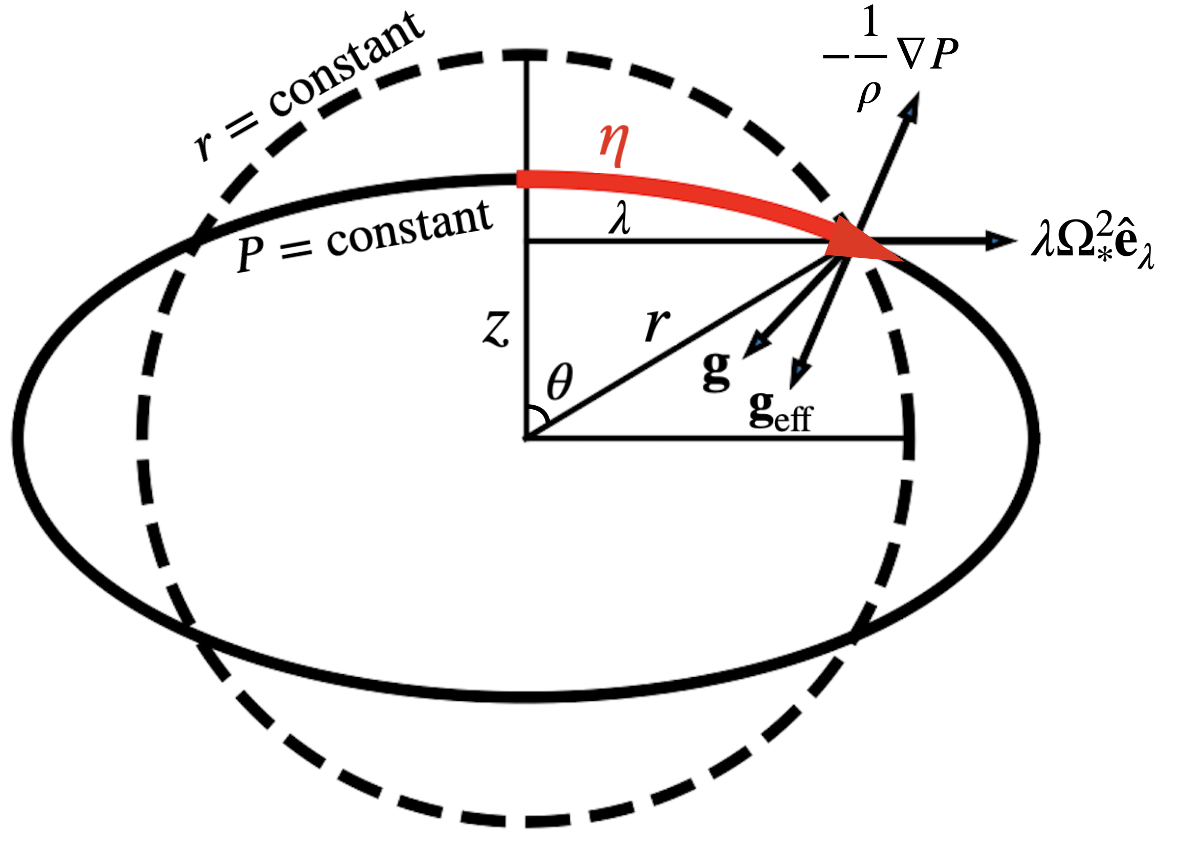
Figure 1: Schematic showing how the GPR balance equation, (5), determines the shape of an oblate star by setting the isobaric surfaces. The relation between the different cylindrical, spherical, and pressure coordinates is shown by the labels $r,\theta,\lambda,z,P$, and $\eta$. Note that $\bm{g}$ points in the general direction shown (not parallel to $-\hat{\bm{e}}_{r}$) because of the oblate centrally concentrated mass.

Because the curl has been taken, the conditions under which stellar thermal wind balance holds may be more restrictive than those associated with GPR balance. We define $Z\equiv|\partial\ln\Omega_{*}^{2}/\partial z|^{-1}$ as the axial scale of variation of $\Omega_{*}^{2}$ and define the thermal wind Rossby, Lorentz, and Ekman numbers:

$${\rm{Ro}}_{\rm{TW}} \equiv\left(\frac{Z}{H}\right){\rm{Ro}}_{\rm{GPR}}=\left(\frac{Z}{H}\right)\left(\frac{U^{2}}{H\lambda\Omega_{*}^{2}}\right),$$ (7a)

$${\rm{Lo}}_{\rm{TW}} \equiv\left(\frac{Z}{H}\right){\rm{Lo}}_{\rm{GPR}}=\left(\frac{Z}{H}\right)\left(\frac{B^{2}}{\mu\rho H\lambda\Omega_{*}^{2}}\right),$$ (7b)

$$\text{and}\ \ \ \ \ {\rm{Ek}}_{\rm{TW}} \equiv\left(\frac{Z}{H}\right){\rm{Ek}}_{\rm{GPR}}=\left(\frac{Z}{H}\right)\left(\frac{\nu U}{H^{2}\lambda\Omega_{*}^{2}}\right).$$ (7c)

The order to which Equation (6) holds is thus set by the largest of ${\rm{Ro}}_{\rm{TW}}$, ${\rm{Lo}}_{\rm{TW}}$, and ${\rm{Ek}}_{\rm{TW}}$.

We assume local thermodynamic equilibrium (LTE) and a known equation of state to rewrite the right-hand side of equation (6) in terms of any other thermodynamic variable. For example, we can instead use the temperature $T$ or the entropy $S$:

$$\frac{1}{\rho}\left(\frac{\partial\rho}{\partial\eta}\right)_{P}=-\beta_{T}\left(\frac{\partial T}{\partial\eta}\right)_{P}=-\frac{\beta_{T}T}{c_{P}}\left(\frac{\partial S}{\partial\eta}\right)_{P},$$ (8)

where $\beta_{T}\equiv-(1/\rho)(\partial\rho/\partial T)_{P}$ is the coefficient of expansion.

Note that equations (6) and (8) make no assumptions about the magnitude of oblateness (i.e., the departures of the thermal variables from spherical symmetry) or the particular equation of state. They are expected to hold anywhere in the star that is in LTE and for which the numbers in equation (7) are small. If the oblateness is small, then $(\partial/\partial\eta)_{P}\rightarrow(1/r)(\partial/\partial\theta)_{P}$, $g_{\rm{eff}}\rightarrow g\equiv|\bm{g}|$, and the thermal variables and $g$ (when not differentiated horizontally) reduce to their spherically symmetric values. Equations (6) and (8) then become:

$$\frac{\partial\Omega_{*}^{2}}{\partial z} =-\frac{\overline{g}}{r^{2}\sin\theta}\frac{1}{\overline{\rho}}\left(\frac{\partial\rho^{\prime}}{\partial\theta}\right)_{P}=\frac{\overline{g}}{r^{2}\sin\theta}\overline{\beta_{T}}\left(\frac{\partial T^{\prime}}{\partial\theta}\right)_{P}$$

$$=\frac{\overline{g}}{r^{2}\sin\theta}\frac{\overline{\beta_{T}}\ \overline{T}}{\overline{c_{P}}}\left(\frac{\partial S^{\prime}}{\partial\theta}\right)_{P},$$ (9)

which is valid to the order of the numbers in equation (7) and (say) the geometric oblateness $f_{*}$. For an ideal gas ($\overline{\beta_{T}}=1/\overline{T}$) and small differential rotation ($\partial\Omega_{*}^{2}/\partial z\approx 2\Omega_{0}\partial\Omega_{*}/\partial z$), equation (2) reduces to equation (4), except that the colatitudinal derivative is now taken along constant $P$ instead of constant $r$. This latter distinction can only be ignored for $S^{\prime}$ in well-mixed convection zones, since there the radial gradient $d\overline{S}/dr$ is the same order as the colatitudinal gradient $(1/r)\partial S^{\prime}/\partial\theta$ (e.g., Balbus et al. 2012; Vasil et al. 2021). Prior studies that estimated the solar aspherical thermal anomalies using the thermal wind equation (e.g., Matilsky et al. 2020; Choudhuri 2021; Vasil et al. 2021) were thus only accurate for $S^{\prime}$, and only in the convection zone not too close to the photosphere (in the outer $\sim$2% of the Sun by radius, $\overline{\beta_{T}}\ \overline{T}/\overline{c_{P}}$ ceases to be a constant).

The relative error between the left-hand sides of equations (4) and (6) (or (2)) is equal to the differential rotation Rossby number ${\rm{Ro}}_{\rm{DR}}\equiv|\Omega_{*}-\Omega_{0}|/\Omega_{*}$. Although ${\rm{Ro}}_{\rm{DR}}\ll 1$ may be true for certain stars, it is not a relevant condition for stellar thermal wind balance. For the Sun in particular, ${\rm{Ro}}_{\rm{DR}}$ can be as high as $\sim$0.3, depending on the choice of $\Omega_{0}$. Apart from increased accuracy, the form $\partial\Omega_{*}^{2}/\partial z$ makes it clear that the thermal wind arises not from the Coriolis force (geostrophy), but from the centrifugal force (axial variations of which tend to produce zonal vorticity).

The fact that the thermal wind $\partial\Omega_{*}^{2}/\partial z$ is a centrifugal term (and should be derived in the inertial frame without introducing the Coriolis force) has been pointed out by numerous authors (e.g., Kitchatinov & Ruediger 1995; Balbus 2009; Lara & Rieutord 2013; Choudhuri 2020). We argue there is a deeper point here, namely that in stars, geostrophy simply cannot hold for a steady zonal flow. On Earth, whose oblate surface is rigid, applying a latitudinal pressure gradient (‘latitudinal’ in the strictly horizontal sense, i.e., perpendicular to $\bm{g}_{\rm{eff}}$) creates a zonal flow according to geostrophy. In a gaseous star or planet, applying an $\eta$ pressure gradient causes the oblateness to adjust until GPR balance is obtained again. In other words, steadily rotating axisymmetric stars do not have nonzero horizontal pressure gradients (see Figure 1), making geostrophic balance in the horizontal direction impossible.

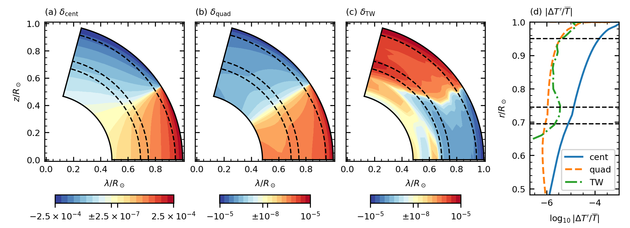
Figure 2: Contributions to the the solar aspherical temperature anomaly: (a) $\delta_{\rm{cent}}$, (b) $\delta_{\rm{quad}}$, and (c) $\delta_{\rm{TW}}$. They have been calculated from the helioseismic inversion of the rotation rate averaged between 1995–2009 (Howe et al., 2005; Howe, 2023). Quantities are shown in the upper half of the meridional plane, excluding latitudes greater than $75^{\circ}$. The colour map is ‘symmetric logarithmic:’ red (blue) tones logarithmically separate positive (negative) values into 9 bins, and one yellow bin contains the values close to zero. The boundaries of each set of bins are given by the colour bar tick labels. Each set of 9 bins spans 3 decades, so neighboring bins are separated by a factor of $\sim$2. (d) Pole-to-equator temperature contrast (|$\Delta\delta|=|\Delta T^{\prime}/\overline{T}|$) from each contribution. In all panels, the boundaries of the tachocline and NSSL are marked by dashed black curves.

3 Aspherical Thermal Anomalies

The full aspherical thermal anomalies can only be determined from the oblateness (GPR) equation (5). By contrast, the curled oblateness equation (2) determines just the baroclinic part of the anomaly due to the thermal wind. We can use the pressure-coordinate formulation to estimate the typical magnitudes of the aspherical thermal anomalies and separate the barotropic and baroclinic contributions. Here we do this for small $f_{*}$, so $(\partial/\partial\eta)_{P}\rightarrow(1/r)(\partial/\partial\theta)_{P}$. For the temperature anomaly $T^{\prime}$, we write the purely mathematical statement:

$$\left(\frac{\partial}{\partial\theta}\right)_{r}\left(\frac{T^{\prime}}{\overline{T}}\right) =\left(\frac{d\ln\overline{T}}{d\ln\overline{P}}\right)\left(\frac{\partial}{\partial\theta}\right)_{r}\left(\frac{P^{\prime}}{\overline{P}}\right)+\left(\frac{\partial}{\partial\theta}\right)_{P}\left(\frac{T^{\prime}}{\overline{T}}\right).$$ (10)

On the right-hand side, the first term is from the barotropic part of the oblateness and the second term from the baroclinic part (thermal wind). Analogous equations can be written for the other thermal anomalies; note that for $S^{\prime}$ in a well-mixed convection zone, the barotropic contribution is negligible.

We write the $\theta$ component of equation (5) as

$$\left(\frac{\partial}{\partial\theta}\right)_{r}\left(\frac{P^{\prime}}{\overline{P}}\right) =\frac{\overline{\rho}}{\overline{P}}(r^{2}\sin\theta\cos\theta\Omega_{*}^{2}+rg_{\theta}),$$ (11)

where $g_{\theta}\equiv\hat{\bm{e}}_{\theta}\cdot\bm{g}$. We expect $g_{\theta}$ to have the same sign and order of magnitude as the centrifugal force term $r\sin\theta\cos\theta\Omega_{*}^{2}$ (Figure 1).

To compare the magnitudes of the two terms in equation (10), we assume an ideal gas ($\overline{\beta_{T}}=1/\overline{T}$) and hydrostatic balance in the spherically symmetric mean variables ($\overline{g}=\overline{P}/\overline{\rho}H_{P}$, where $H_{P}\equiv-(d{\ln\overline{P}}/dr)^{-1}$ is the local pressure scale-height). Using equations (2) and (11), we estimate:

$$\delta_{\rm{bar}} \equiv\left(\frac{d\ln\overline{T}}{d\ln\overline{P}}\right)\int\left(\frac{\partial}{\partial\theta}\right)_{r}\left(\frac{P^{\prime}}{\overline{P}}\right)d\theta\sim\left(\frac{r}{H_{P}}\right)\left(\frac{r\sin\theta\cos\theta\Omega_{*}^{2}}{\overline{g}}\right),$$ (12a)

$$\delta_{\rm{TW}} \equiv\int\left(\frac{\partial}{\partial\theta}\right)_{P}\left(\frac{T^{\prime}}{\overline{T}}\right)d\theta\sim\left(\frac{r}{Z}\right)\left(\frac{r\sin\theta\Omega_{*}^{2}}{\overline{g}}\right),$$ (12b)

where we have defined $\delta_{\rm{bar}}$ and $\delta_{\rm{TW}}$ as the temperature anomalies from the barotropic part of the oblateness and the baroclinic part (thermal wind), respectively. Both anomalies are the same magnitude as the oblateness itself, since $r\Omega_{*}^{2}/\overline{g}\sim(r/R_{*})^{3}m$ (where $R_{*}$ is the stellar radius and $m\equiv R_{*}\Omega_{*}^{2}/\overline{g}_{\rm{surf}}$, with $\overline{g}_{\rm{surf}}$ the surface gravity) and in general, $m\sim f_{*}$ (e.g., Collins 1963). However, since $\delta_{\rm{TW}}/\delta_{\rm{bar}}\sim H_{P}/Z$, $\delta_{\rm{TW}}$ is often significantly smaller than $\delta_{\rm{bar}}$, except in regions of very strong axial shear (small $Z$). From equation (12a), we expect $\delta_{\rm{bar}}$ to be largest near the stellar surface (if the GPR approximation still holds there), since $H_{P}$ becomes very small. Prior estimates of the solar temperature anomaly—which considered only the thermal wind equation—thus missed the dominant barotropic contribution, as we show explicitly in the following section.

4 The solar temperature anomaly

The Sun’s aspherical thermal anomalies (e.g., $T^{\prime}$ and $S^{\prime}$) are of fundamental importance. The gradients of $S^{\prime}$ may determine how efficient the convection is according to mixing-length theory and thus how the radial energy transport varies with latitude (e.g., Featherstone & Miesch 2015). The structure of $T^{\prime}$ determines the energy transport by the meridional circulation (e.g., Matilsky et al. 2020) and is also closely related to variations in the sound speed, which may be directly measurable via helioseismology. Observations of the solar emissive flux reveal a slightly superluminous pole (Rast et al., 2008), yielding a pole-to-equator relative difference in emissive flux of $\Delta I/I_{0}\sim 2\times 10^{-3}$, or a difference in effective temperature of $\Delta T_{\rm{eff}}\sim 2.5$ K. It is thus natural to speculate that $\Delta T_{\rm{eff}}$ might be an ‘imprint’ of the interior temperature anomaly (e.g., Choudhuri 2021).

Table 1: Left two columns: volume-averages of $\Delta T^{\prime}/\overline{T}$ over the tachocline and the NSSL. Right-most column: volume-average of $\Delta T^{\prime}$ over the NSSL.

	$\Delta T^{\prime}/\overline{T}=\Delta\delta$		$\Delta T^{\prime}$
	tachocline	NSSL	NSSL
centrifugal	$-1.1\times 10^{-5}$	$-5.7\times 10^{-4}$	$-39$ K
quadrupole	$-1.0\times 10^{-6}$	$-1.2\times 10^{-5}$	$-0.85$ K
thermal wind	$\gtrsim 3.2\times 10^{-6}$	$1.0\times 10^{-5}$	$1.1$ K

An obvious way to infer the thermal anomalies is to assume GPR and thermal wind balance and use equation (12), along with the helioseismically measured solar rotation rate in equations (2) and (11). However, prior calculations have considered only the thermal wind equation (2) (e.g., Vasil et al. 2021; Jha & Choudhuri 2021) and excluded the barotropic oblateness contribution. Furthermore, no distinction was made between $(\partial/\partial\theta)_{P}$ and $(\partial/\partial\theta)_{r}$, meaning the calculations only yielded $S^{\prime}$ correctly, and only in the convection zone. Although Matilsky et al. (2020) attempted to calculate $T^{\prime}$ (summing both the thermal wind and barotropic parts), we used an incorrect form of equation (11).

Here we provide a new calculation of the relative temperature anomaly $\delta\equiv T^{\prime}/\overline{T}$ ($=\delta_{\rm{bar}}+\delta_{\rm{TW}}$), using pressure coordinates. The most uncertainty comes from $g_{\theta}$, which relates to the distribution of matter in the oblate solar core and has not been measured. To lowest order, we assume that the quadrupole moment dominates and write $g_{\theta}\approx(3/2)J_{2}(GM_{\odot}R_{\odot}^{2}/r^{4})\sin\theta\cos\theta$, where $J_{2}$ is the gravitational quadrupole moment, $G$ the gravitational constant, $M_{\odot}$ the solar mass, and $R_{\odot}$ the solar radius. Equation (11) then becomes

$$\left(\frac{\partial}{\partial\theta}\right)_{r}\left(\frac{P^{\prime}}{\overline{P}}\right) =\frac{\overline{\rho}}{\overline{P}}\left[r^{2}\Omega_{*}^{2}+\frac{3}{2}(R_{\odot}^{2}\Omega_{\odot}^{2})\left(\frac{J_{2}}{m_{\odot}}\right)\left(\frac{R_{\odot}}{r}\right)^{3}\right]\sin\theta\cos\theta,$$ (13)

where $\Omega_{\odot}\equiv 2.7\times 10^{-6}\ \rm{rad\ s^{-1}}$ (or $\Omega_{\odot}/2\pi\equiv 430$ nHz) is the the approximate solid-body rotation rate of the radiative zone and $m_{\odot}\equiv R_{\odot}^{3}\Omega_{\odot}^{2}/GM_{\odot}=1.9\times 10^{-5}$.

Using equation (13) in equation (12a), we write $\delta_{\rm{bar}}=\delta_{\rm{cent}}+\delta_{\rm{quad}}$, defining the separate contributions from the centrifugal force and quadrupole. $J_{2}$ can be estimated from the rotation rate by solving equation (5) simultaneously with the Poisson equation for the gravitational potential (e.g., Dicke 1967; Ulrich & Hawkins 1981). Using the helioseismic rotation law then yields $J_{2}\approx 2.2\times 10^{-7}$ (Pijpers, 1998; Armstrong & Kuhn, 1999). Note that $(3/2)J_{2}/m_{\odot}\approx 0.017$, so that for the Sun, $\delta_{\rm{quad}}\ll\delta_{\rm{cent}}$, except deep in the interior.

We take the spherically averaged quantities from model S (Christensen-Dalsgaard et al., 1996). We use equations (2) and (13) in (12) to find $\delta_{\rm{cent}}$, $\delta_{\rm{quad}}$, and $\delta_{\rm{TW}}$. We set the integration constants so that each $\delta_{(\cdots)}$ separately has no spherical mean (excluding the region above $75^{\circ}$ latitude). For $T^{\prime}=T^{\prime}(r,\theta)$, we also define the pole-to-equator temperature contrast: $\Delta T^{\prime}(r)\equiv T^{\prime}(r,\pi/12)-T^{\prime}(r,\pi/2)$ and $\Delta\delta=\Delta T^{\prime}/\overline{T}$ (positive for for a pole hotter than the equator). The result is shown in figure 2 and table 1. In presenting these results, we refer to the Sun’s two radial shear layers: the tachocline (radial boundaries at $(0.72\pm 0.025)R_{\odot}$) and the near-surface shear layer (NSSL; boundaries at $0.95R_{\odot}$, $R_{\odot}$).

The biggest contribution is $\delta_{\rm{cent}}$ (figure 2a). This term would make the equatorial regions slightly hotter than the polar regions ($\Delta T^{\prime}<0$), with $|\Delta T^{\prime}/\overline{T}|$ increasing from $\sim$$10^{-5}$ in the tachocline to $\sim$$6\times 10^{-4}$ in the NSSL (table 1). Helioseismic measurements so far have been sensitive to asphericity on the order of $\sim$$10^{-4}$ in the relative sound speed anomaly (e.g., Antia & Basu 2001), which should match $\delta$ where the gas is ideal. Thus, $\delta_{\rm{cent}}$ (and not $\delta_{\rm{TW}}$, which is $\sim$$10^{-5}$ in the NSSL) is the only contribution currently measurable by helioseismology, and only in the outermost layers (e.g., the NSSL). To further complicate a possible future measurement of thermal wind balance, $\delta_{\rm{TW}}$ and $\delta_{\rm{quad}}$ appear to be nearly equal and opposite above $r\approx 0.8R_{\odot}$. Unless $J_{2}$ is known accurately, subtracting an estimated $\delta_{\rm{quad}}$ from a measured $\delta$ could uncover false thermal wind balance.

Interestingly, Antia & Basu (2001) measure a sound speed in the NSSL that is smaller near the equator than near the poles (i.e., $\Delta T^{\prime}>0$). This implies that possibly GPR balance does not hold in the NSSL, or (as mentioned by Antia & Basu 2001), the measurements reflect the interior magnetic field, not the sound speed variations.

Deep in the Sun, the helioseismically measured $Z$ is really an upper bound, set by the large size of the inversion kernels (e.g., Howe 2009, p. 31). This makes our estimated value of $\delta_{\rm{TW}}$ a lower bound. It has been proposed that the tachocline is substantially thinner than the inversion kernels (e.g., Elliott 1997), but the true thickness $\Gamma$ is still unknown and would have important consequences for the global solar dynamo and the tachocline confinement problem (e.g., Miesch 2005; Matilsky et al. 2022). If we accept thermal wind balance a priori, then a precisely measured $\delta$ in the tachocline (after subtracting the $\delta_{\rm{cent}}$ and $\delta_{\rm{quad}}$ estimated here) would yield the true value of $\delta_{\rm{TW}}$, and hence $\Gamma$. For example, the inversion considered here (Howe et al., 2005; Howe, 2023) gives $\Gamma\lesssim 0.05R_{\odot}$ and $\Delta\delta_{\rm{TW}}\gtrsim 3\times 10^{-6}$ (table 1). If a future measurement of the sound speed anomaly were to yield $\Delta\delta\approx 10^{-5}$ ($\Delta\delta_{\rm{TW}}\approx 2\times 10^{-5}$), that would imply $\Gamma\approx 0.01R_{\odot}$.

We point out that none of the values in table 1 (either dimensional or non-dimensional) closely match the $\Delta I/I_{0}\sim 2\times 10^{-3}$ or $\Delta T_{\rm{eff}}\sim 2.5$ K reported in Rast et al. (2008). Even ignoring the discrepancies in sign, the magnitudes of our non-dimensional values are all too low (as are the dimensional $|\Delta T^{\prime}|$ from the thermal wind and quadrupole), while $|\Delta T^{\prime}|$ from the centrifugal force is too high. This indicates that the interior temperature anomaly does not imprint directly onto the surface. This may not be too surprising (and does necessarily mean GPR or thermal wind balance breaks down in the NSSL), since it is still not well-understood how the interior $T^{\prime}$ and $S^{\prime}$ determine the energy flux (and thus the observed $\Delta T_{\rm{eff}}$, which really measures asphericity in the outward energy flux at the photosphere).

Apart from measuring the thermal anomalies, the validity of solar GPR and thermal wind balance could be assessed by estimating the relevant non-dimensional numbers in equation (7) from the expected Reynolds and Maxwell stresses. In the NSSL, for example, supergranulation gives $U\sim 100\ \rm m\ s^{-1}$ and $H\sim 30$ Mm (e.g., Rincon & Rieutord 2018). Using $\lambda\sim 500$ Mm, $\Omega_{*}\sim 3\times 10^{-6}\ \rm rad\ s^{-1}$, and $Z\sim 10^{3}$ Mm (for $Z$, see Matilsky 2023) gives ${\rm{Ro}}_{\rm{GPR}}\sim 0.07$ and ${\rm{Ro}}_{\rm{TW}}\sim 2.5$. We thus might expect the NSSL to be in GPR balance, but not thermal wind balance (ignoring for now the Maxwell stress since its value is poorly constrained). Of course, this estimate implicitly assumes that the meridional components of the velocity from supergranulation are perfectly correlated; a poor correlation might yield ${\rm{Ro}}_{\rm{TW}}\ll 1$, and then thermal wind balance might still hold.

5 Conclusions

We derive the equations of GPR balance and the corollary of stellar thermal wind balance, which we contrast with the different equation of terrestrial thermal wind balance. We also derive the non-dimensional numbers that must be small to make each equation valid. We show that the stellar thermal wind is really a consequence of the centrifugal force (oblateness) and not of the Coriolis force (geostrophy). Furthermore, the aspherical thermal anomalies due to the barotropic parts of the oblateness (here we consider the contributions from the centrifugal force and gravitational quadrupole moment) are necessarily the same order of magnitude as the baroclinic anomaly from the thermal wind, and often substantially larger.

Using pressure coordinates, we estimate the temperature anomaly for the Sun, separating the contributions from the centrifugal force, gravitational quadrupole, and thermal wind. We find that verifying or falsifying thermal wind balance by measuring the solar temperature anomaly heloseismically may not be possible. On the other hand, measuring the anomaly to an improved precision of $\sim$$10^{-5}$ (and simply accepting thermal wind balance for the deep interior) may yield a new way to bracket the width of the tachocline. Finally, it is not clear exactly how measurements of surface emissive flux (e.g., Rast et al. 2008) connect to the interior thermal anomalies. Until this connection is well-understood (or the interior Reynolds and Maxwell stresses are more reliably estimated), it is still an open question whether GPR and thermal wind balance hold everywhere in the Sun.

Data Availability

The helioseismic inversion of the solar rotation rate is publicly available via Zenodo (Howe, 2023). Model S is available at https://users-phys.au.dk/~jcd/solar_models/. The solar temperature anomalies, entropy anomalies, and $Z$ (with a more complete description of numerical methods) are publicly available via Zenodo (Matilsky, 2023).

References

- Antia & Basu (2001) Antia H. M., Basu S., 2001, ApJ, 559, L67
- Armstrong & Kuhn (1999) Armstrong J., Kuhn J. R., 1999, ApJ, 525, 533
- Aurnou & Aubert (2011) Aurnou J. M., Aubert J., 2011, PEPI, 187, 353
- Balbus (2009) Balbus S. A., 2009, MNRAS, 395, 2056
- Balbus et al. (2012) Balbus S. A., Latter H., Weiss N., 2012, MNRAS, 420, 2457
- Brun et al. (2010) Brun A. S., Antia H. M., Chitre S. M., 2010, A&A, 510, A33
- Chao (2006) Chao B. F., 2006, CRGeo, 338, 1123
- Choudhuri (2020) Choudhuri A. R., 2020, SCPMA, 64
- Choudhuri (2021) Choudhuri A. R., 2021, SoPh, 296
- Christensen-Dalsgaard et al. (1996) Christensen-Dalsgaard J., et al., 1996, Sci., 272, 1286
- Collins (1963) Collins G. W., 1963, ApJ, 138, 1134
- Dicke (1967) Dicke R. H., 1967, ApJ, 149, L121
- Elliott (1997) Elliott J. R., 1997, A&A, 327, 1222
- Featherstone & Miesch (2015) Featherstone N. A., Miesch M. S., 2015, ApJ, 804, 67
- Goldreich & Schubert (1968) Goldreich P., Schubert G., 1968, ApJ, 154, 1005
- Howe (2009) Howe R., 2009, LRSP, 6, 1
- Howe (2023) Howe R., 2023, Mean solar rotation profile from GONG splittings 1995-2009, doi:10.5281/ZENODO.8171572
- Howe et al. (2005) Howe R., Christensen-Dalsgaard J., Hill F., Komm R., Schou J., Thompson M. J., 2005, ApJ, 634, 1405
- Jha & Choudhuri (2021) Jha B. K., Choudhuri A. R., 2021, MNRAS, 506, 2189
- Kitchatinov & Ruediger (1995) Kitchatinov L. L., Ruediger G., 1995, A&A, 299, 446
- Lara & Rieutord (2013) Lara F. E., Rieutord M., 2013, A&A, 552, A35
- Matilsky (2023) Matilsky L. I., 2023, Dataset for MNRAS Letter: The stellar thermal wind as a consequence of oblateness, doi:10.5281/ZENODO.8176830
- Matilsky et al. (2020) Matilsky L. I., Hindman B. W., Toomre J., 2020, ApJ, 898, 111
- Matilsky et al. (2022) Matilsky L. I., Hindman B. W., Featherstone N. A., Blume C. C., Toomre J., 2022, ApJL, 940, L50
- Miesch (2005) Miesch M. S., 2005, LRSP, 2, 1
- Pedlosky (1987) Pedlosky J., 1987, Geophysical Fluid Dynamics. Springer, New York, doi:10.1007/978-1-4612-4650-3
- Pijpers (1998) Pijpers F. P., 1998, MNRAS, 297, L76
- Rast et al. (2008) Rast M. P., Ortiz A., Meisner R. W., 2008, ApJ, 673, 1209
- Rincon & Rieutord (2018) Rincon F., Rieutord M., 2018, LRSP, 15, 6
- Thompson et al. (2003) Thompson M. J., Christensen-Dalsgaard J., Miesch M. S., Toomre J., 2003, ARA&A, 41, 599
- Ulrich & Hawkins (1981) Ulrich R. K., Hawkins G. W., 1981, ApJ, 246, 985
- Vallis (2017) Vallis G. K., 2017, Atmospheric and Oceanic Fluid Dynamics. Cambridge University Press, doi:10.1017/9781107588417
- Vasil et al. (2021) Vasil G. M., Julien K., Featherstone N. A., 2021, PNAS, 118