Jointly Improving the Sample and Communication Complexities in Decentralized Stochastic Minimax Optimization

Abstract

In this work, we propose a novel single-loop decentralized algorithm called DGDA-VR for solving the stochastic nonconvex strongly-concave minimax problem over a connected network of $M$ agents. By using stochastic first-order oracles to estimate the local gradients, we prove that our algorithm finds an $\epsilon$-accurate solution with $\mathcal{O}(\epsilon^{-3})$ sample complexity and $\mathcal{O}(\epsilon^{-2})$ communication complexity, both of which are optimal and match the lower bounds for this class of problems. Unlike competitors, our algorithm does not require multiple communications for the convergence results to hold, making it applicable to a broader computational environment setting. To the best of our knowledge, this is the first such algorithm to jointly optimize the sample and communication complexities for the problem considered here.

1 Introduction

This paper considers a connected network $\mathcal{G}=(\mathcal{V},\mathcal{E})$ of $M$ agents which cooperatively solve

$$\min_{\mathbf{x}\in\mathbb{R}^{{\color[rgb]{0,0,0}d}}}\max_{\mathbf{y}\in\mathbb{R}^{m}}f(\mathbf{x},\mathbf{y})\triangleq\frac{1}{M}\sum_{i=1}^{M}f_{i}(\mathbf{x},\mathbf{y}),$$ (1)

where $f_{i}:{\color[rgb]{0,0,0}\mathbb{R}^{d}\times\mathbb{R}^{m}}\rightarrow\mathbb{R}$ are smooth and possibly nonconvex in $\mathbf{x}\in\mathbb{R}^{d}$ and are strongly-concave in $\mathbf{y}\in\mathbb{R}^{m}$ for $i=1,2,...,M$. Furthermore, each agent-$i$ can only access unbiased stochastic gradients $\tilde{\nabla}f_{i}$ rather than exact gradients $\nabla f_{i}$ and we assume that $\{\tilde{\nabla}f_{i}\}_{i\in\mathcal{V}}$ have finite variances, uniformly bounded by some $\sigma>0$. The set $\mathcal{V}=\{1,2,\dots,M\}$ indexes the $M$ agents and $(i,j)\in\mathcal{E}\subseteq\mathcal{V}\times\mathcal{V}$ only if agent $i$ can send information to agent $j$. Minimax optimization has garnered recent interest due to applications in many machine learning settings such as adversarial training [12, 23], distributionally robust optimization [28, 44], reinforcement learning [56], and fair machine learning [31]. The problem in (1) arises naturally when the data is physically distributed among many agents or is too large to store on a single computing device [46]. It is well known that centralized methods suffer from communication bottlenecks on the parameter server [20, 44] and potential data privacy violations [42]; hence, decentralized methods have emerged as a practical alternative to overcome these issues.

In a decentralized setting, $f_{i}$ and its stochastic gradient oracle can only be accessed by agent-$i$, and thus in order for the $M$ agents to collaboratively solve (1), each agent-$i$ will make a local copy, denoted as $(\mathbf{x}_{i},\mathbf{y}_{i})$, of the primal-dual variable $(\mathbf{x},\mathbf{y})$ and communicate the local variables and gradient information with its (1-hop) neighbors. In this way, (1) can be reformulated equivalently into the following problem in a decentralized format:

$$\begin{split}&\min_{\{\mathbf{x}_{i}\}_{{\color[rgb]{0,0,0}i\in\mathcal{V}}}}\max_{\{\mathbf{y}_{i}\}_{{\color[rgb]{0,0,0}i\in\mathcal{V}}}}\frac{1}{{\color[rgb]{0,0,0}|\mathcal{V}|}}\sum_{{\color[rgb]{0,0,0}i\in\mathcal{V}}}f_{i}(\mathbf{x}_{i},\mathbf{y}_{i})\\ \text{ s.t. }&\mathbf{x}_{i}=\mathbf{x}_{j},\quad\mathbf{y}_{i}=\mathbf{y}_{j},\enskip\forall\,(i,j)\in\mathcal{E}.\end{split}$$ (2)

Consensus among the agents is then enforced through the use of a mixing matrix encoding the topology of $\mathcal{G}$, discussed in detail later.

Although there are existing decentralized algorithms for stochastic nonconvex-strongly-concave minimax problems, the existing work [23, 4] requires multi-communication rounds at each iteration; hence, they can be analyzed as a centralized algorithm with inexact gradients. In a multi-agent setting, methods requiring multi-communication rounds per iteration are not desired as they require more strict coordination among the agents while single round communication methods are much easier to implement. We will design a decentralized algorithm for (1) or equivalently (2) that only requires a single communication round per iteration. Although another recent work [44] attempted the same problem and also proposed a decentralized algorithm with a single round of communication per iteration, we noticed that its proof has a fundamental issue and the claimed complexity results do not hold — we explain this problem in detail when we compare our results with the existing work in Section 2. In addition, the communication complexity result of the algorithm in [44] will intrinsically be the same order as its sample complexity result and cannot be optimal. In contrast, the algorithm that we design can achieve an optimal complexity result for both sample complexity and communication complexity in terms of the dependence on a given tolerance.

Contributions.

Our contributions are two-fold. First, we propose a decentralized stochastic gradient-type method, called black, for solving (1) or equivalently (2). At every iteration of the method, each agent-$i$ performs a local stochastic gradient descent step for $\mathbf{x}_{i}$ and a local stochastic gradient ascent step for $\mathbf{y}_{i}$, along a tracked (global) stochastic gradient direction. black needs only a single communication round per iteration for neighbor (weighted) averaging local variables and tracked stochastic gradient information.

Second, we show that when each agent uses a SPIDER-type stochastic gradient estimator [10], which is a variant of SARAH [29], black can, in a decentralized manner, generate $\{\mathbf{z}_{i}(\epsilon)\}_{i\in\mathcal{V}}$ with $\mathbf{z}_{i}(\epsilon)\triangleq\big{(}\mathbf{x}_{i}(\epsilon),\mathbf{y}_{i}(\epsilon)\big{)}$ such that the local decisions $\{\mathbf{z}_{i}(\epsilon)\}_{i\in\mathcal{V}}$ and their average $(\bar{\mathbf{x}}_{\epsilon},\bar{\mathbf{y}}_{\epsilon})=\bar{\mathbf{z}}_{\epsilon}=\frac{1}{|\mathcal{V}|}\sum_{i\in\mathcal{V}}\mathbf{z}_{i}(\epsilon)$ have the following properties:

1. $\bar{\mathbf{x}}_{\epsilon}$ is an $\epsilon$-stationary point of the primal function $\Phi(\cdot)\triangleq\max_{\mathbf{y}}f(\cdot,\mathbf{y})$, i.e., $\mathbf{E}[\|\nabla\Phi(\bar{\mathbf{x}}_{\epsilon})\|]\leq\epsilon$;

2. $\bar{\mathbf{y}}_{\epsilon}$ is an $\mathcal{O}(\epsilon)$-optimal-response to $\bar{\mathbf{x}}_{\epsilon}$, i.e., $\mathbf{E}[\|\bar{\mathbf{y}}_{\epsilon}-\mathbf{y}^{*}(\bar{\mathbf{x}}_{\epsilon})\|]=\mathcal{O}(\epsilon)$, where $\mathbf{y}^{*}(\bar{\mathbf{x}}_{\epsilon})=\operatorname*{argmax}_{\mathbf{y}}f(\bar{\mathbf{x}}_{\epsilon},\mathbf{y})$;

3. $\{\mathbf{z}_{i}(\epsilon)\}_{i\in\mathcal{V}}$ has $\mathcal{O}(\epsilon)$-consensus-violation, i.e., $\mathbf{E}[\sum_{i\in\mathcal{V}}\|\mathbf{z}_{i}(\epsilon)-\bar{\mathbf{z}}_{\epsilon}\|^{2}]=\mathcal{O}(\epsilon^{2})$;

4. this computation requires $\mathcal{O}((1-\rho)^{-2}\epsilon^{-2})$ communication among neighboring nodes, which employ $\mathcal{O}(\sigma(1-\rho)^{-2}\epsilon^{-3})$ stochastic oracle calls, i.e., the sampling complexity — here, $\rho\in[0,1)$ measures the connectivity of the underlying communication network, and a smaller $\rho$ means a more connected network. The orders $\mathcal{O}(\epsilon^{-2})$ for communication rounds and $\mathcal{O}(\epsilon^{-3})$ for stochastic oracles both match with existing lower bounds [35, 1].

Notation and definitions.

Throughout the paper, we use bold lower-case letters $\mathbf{x},\mathbf{y},\ldots$ to denote vectors and upper-case letters $X,Y,\ldots$ to denote matrices. $\|\cdot\|$ denotes the Euclidean norm for a vector. $\|\cdot\|_{F}$ and $\|\cdot\|_{2}$ denote the Frobenius norm, and the spectral norm of a matrix, respectively. The symbols $\mathbf{I}$ and $\mathbf{1}$ denote the identity matrix and the column vector with all elements $1$, respectively. The symbol $\mathbf{E}$ is used for expectation. $W$ represents a mixing matrix and $\Pi\triangleq\frac{1}{M}\mathbf{1}\mathbf{1}^{\top}\in\mathbb{R}^{M\times M}$ the averaging matrix. We let $\mathbb{N}^{+}\triangleq\mathbb{N}/\{0\}$. Given $M\in\mathbb{N}^{+}$, $[M]$ denotes the integer set $\{1,2,..,M\}$. Given a random variable $\xi$, for any $i\in[M]$, $\tilde{\nabla}f_{i}(\mathbf{x},\mathbf{y};\xi)$ denotes an unbiased estimator of $\nabla f_{i}(\mathbf{x},\mathbf{y})$, of which properties are stated in Assumptions 4 and 5. We interchangeably use $\mathbb{R}^{d}\times\mathbb{R}^{m}=\mathbb{R}^{d+m}$ when it is convenient to define the inputs to $f_{i}$ as a single vector. We will use the more compact matrix variables for (2)

$$X\triangleq[\mathbf{x}_{1},\ldots,\mathbf{x}_{M}]^{\top},\ Y\triangleq[\mathbf{y}_{1},\ldots,\mathbf{y}_{M}]^{\top},\ Z\triangleq[X,Y].$$

Organization.

In Section 2, we briefly discuss the previous work on decentralized minimax problems related to ours. After we give some important definitions and state our assumptions in Section 3, we describe our proposed method and main results in detail in Section 4 and we discuss the overview of convergence analysis in Section 5. Finally, we test our method against the SOTA methods employing variance reduction on a distributed logistic regression problem with a non-convex regularizer in Section 6.

2 Related Work

Table 1: Representative decentralized minimax optimization methods. The P column gives the problem setting between finite-sum (FS) or stochastic (S); for FS setting, we let $n$ denote the number of component functions. The U column gives whether stochastic (S) or deterministic (D) gradients are used. Some works do not make the dependence upon the spectral gap or condition number clear; we use constants $a,b,c,d>0$ with subscripts $s$ and $c$ to denote whether or not these unknowns are related to the sample or communication complexities, respectively. An ✗ in the final column indicates there is no special requirement for the theoretical results to hold. ^†GT-DA considers a slightly different problem than (2) as consensus is only enforced on $\{\mathbf{x}_{i}\}$ or $\{\mathbf{y}_{i}\}$; additionally, GT-DA performs deterministic updates, hence $\sigma$ does not appear in the convergence results. ^⋄GT-SRVR can remove the dependence upon $\sigma$ by computing a full gradient periodically. ^¶DSGDA uses a variance reduction technique which removes the bounded variance assumption (hence $\sigma$ does not appear), however, it is unclear whether this technique can be extended to the stochastic setting. ^‡DPOSG considers the nonconvex-nonconcave problem, hence $\kappa$ is undefined for this setting; additionally, $t>1$ represents the required number of communications per iteration.

Method	P	U	Samp. Comp.	Comm. Comp.	Requirement
GT-DA [41]†	FS	D	$\tilde{\mathcal{O}}\left(\frac{n\kappa^{a_{s}}}{(1-\rho)^{b_{s}}\varepsilon^{2}}\right)$	$\tilde{\mathcal{O}}\left(\frac{\kappa^{a_{c}}}{(1-\rho)^{b_{c}}\varepsilon^{2}}\right)$	mult. $\mathbf{y}$-update
GT-SRVR [56]	FS	S	$\mathcal{O}\left(n+\frac{\sqrt{n}\kappa^{c_{s}}}{(1-\rho)^{d_{s}}\varepsilon^{2}}\right)^{\diamond}$	$\mathcal{O}\left(\frac{\kappa^{c_{c}}}{(1-\rho)^{d_{c}}\varepsilon^{2}}\right)$	✗
DSGDA [11]	FS	S	$\mathcal{O}\left(\frac{\sqrt{n}\kappa^{3}}{(1-\rho)^{2}\varepsilon^{2}}\right)^{\P}$	$\mathcal{O}\left(\frac{\kappa^{3}}{(1-\rho)^{2}\varepsilon^{2}}\right)$	✗
DPOSG [23]	S	S	$\mathcal{O}\left(\frac{\sigma^{2}}{(1-\rho^{t})^{2}\varepsilon^{12}}\right)^{\ddagger}$	$\mathcal{O}\left(\frac{\sigma^{2}}{(1-\rho^{t})^{2}\varepsilon^{12}}\right)^{\ddagger}$	mult. comm.
DREAM [4]	S	S	$\mathcal{O}\left(\frac{\kappa^{3}\sigma}{\varepsilon^{3}}\right)$	$\mathcal{O}\left(\frac{\kappa^{2}}{\sqrt{1-\rho}\varepsilon^{2}}\right)$	mult. comm.
Ours	S	S	$\mathcal{O}\left(\frac{\kappa^{3}\sigma}{\min\{1/\kappa,(1-\rho)^{2}\}\epsilon^{3}}\right)$	$\mathcal{O}\left(\frac{\kappa^{2}}{\min\{1/\kappa,(1-\rho)^{2}\}\varepsilon^{2}}\right)$	✗

We provide a brief literature review of decentralized optimization methods (specifically for nonconvex and stochastic problems), and discuss both centralized and decentralized methods for minimax problems.

Decentralized optimization.

D-PSGD [20] first advocated for the use of decentralized methods and provided convergence analysis for a stochastic gradient-type method. $D^{2}$ [37] improved the analysis of D-PSGD to allow for data heterogeneity. More recently, gradient tracking has been utilized to further enhance the convergence rate of new methods; see [25, 52, 15, 47] for further discussions. Variance reduction methods that mimic updates from the SARAH [30] and SPIDER [43] methods provide optimal gradient complexity results at the expense of large batch computations; examples include D-SPIDER-SFO [33], D-GET [36], GT-SARAH [48], DESTRESS [17]. To avoid the large batch requirement of these methods, the STORM [7, 50] and Hybrid-SGD [39] methods have also been adapted to the decentralized setting; see GT-STORM [55] and GT-HSGD [46]. Both types of variance reduction have recently been extended to include a proximal term in ProxGT-SR-O/E [45] and DEEPSTORM [27]. There are many other decentralized methods which handle various problem settings, but an exhaustive discussion is beyond the scope of this work; we refer interested readers to the references in the above works for more details.

Minimax optimization.

Before discussing purely decentralized minimax optimization methods, we first provide a brief overview of centralized minimax optimization methods. In recent years, a significant amount of work has been proposed [5, 14, 21, 22, 24, 32, 38, 58, 51]. In general, two cases are considered: (i) the deterministic setting, where the partial gradients of $f_{i}$ are exactly available; (ii) the stochastic setting, where only stochastic estimates of the gradients are available. Moreover, the lower complexity bounds have also been studied for centralized minimax algorithms in [53, 54, 18] – these type of bounds are useful as they indicate a potential room for improvement in algorithm design. Our focus in this paper will be mainly on the stochastic setting, which is more relevant and more applicable to large-scale machine learning (ML) problems. Indeed, due to large-dimensions and the sheer size of the modern datasets, it is either infeasible or impractical to compute exact gradients in practice and gradients are often estimated stochastically based on mini-batches (randomly sampled subset of data points) as in the case of stochastic gradient-type algorithms. Therefore, more methods employing variance reduction have been considered to improve the performance of the stochastic minimax algorithms, e.g., see [49, 13, 26, 57]. In this paper, to control the noise accumulation, we propose black, a decentralized method employing the SPIDER variance reduction technique [10], a variant of SARAH [29, 29].

For the decentralized setting, we summarize some representative work for solving the minimax problem in Table 1. The method GT-DA [41] is proposed for a slightly modified version of (2) in the deterministic setting; this method only enforces consensus on the $\mathbf{x}_{i}$ variables and as such requires the $\mathbf{y}$-subproblem be solved to an increasing accuracy at each iteration. GT-SRVR [56] is closely related to black, our proposed algorithm; that said, the analysis for GT-SRVR is only provided for the finite-sum problem and further, the dependence upon important parameters such as $\kappa$ and $\rho$ is unclear. Similarly, DSGDA [11] is proposed for the finite-sum setting, and employs a stochastic gradient estimator from [19], for which it is unclear on how to theoretically extend to the general stochastic setting. For the purely stochastic case, DPSOG [23] is a general method that solves the nonconvex-nonconcave problem, however, its oracle complexity is sub-optimal. Furthermore, DPSOG requires multiple communications per each iteration in order to guarantee the convergence to a stationary point.

Comparison with DM-HSGD and DREAM.

We provide a more detailed comparison of black to two closely related methods: DM-HSGD [44] and DREAM [4]. The recent DM-HSGD [44] algorithm adapts the STORM-type update to the decentralized minimax setting; however, there are several critical errors in their proof which impact their results. First, their equation (28) does not hold with the given choice of $\theta$. In fact, $\theta$ must depend on $L$, for which it is not clear whether their convergence analysis will go through if one chooses $\theta=\Theta(1/L)$ to make their equation (28) valid, e.g., in this scenario the coefficient of $\mathbb{E}\|\bar{u}^{t}\|$ becomes positive and cannot be dropped from the final bound while their convergence analysis requires this term to be dropped. Second, the algorithm is claimed to solve the minimax problem in (2) such that $\mathbf{y}\in\mathcal{Y}$ for a convex set $\mathcal{Y}\subseteq\mathbb{R}^{m}$; however, equation (29) in their Lemma 5 cannot hold unless $\mathcal{Y}\triangleq\mathbb{R}^{m}$ which means that at best, their analysis is only applicable to (2) without simple constraint sets. The recent DREAM [4] is similar to our method in terms of the variance reduction technique used to reduce the sample complexity. However, their proof requires the use of multiple communications for their Lemma 3 to hold (see their equations (19) and (22)); our proof technique removes such a requirement so that for any given connected network topology, our algorithm black is guaranteed to converge.

3 Preliminaries

Throughout the paper, for notational convenience, we define $\mathbf{z}=(\mathbf{x},\mathbf{y})\in\mathbb{R}^{d+m}$ to be the concatenation of the $\mathbf{x}$ and $\mathbf{y}$ variables. We start with some basic definitions.

Definition 1.

A differentiable function $r$ is $L$-smooth if $\exists L>0$ such that $\|\nabla r(\mathbf{z})-\nabla r(\mathbf{z}^{\prime})\|\leq L\|\mathbf{z}-\mathbf{z}^{\prime}\|$, $\forall\,\mathbf{z},\mathbf{z}^{\prime}$.

Definition 2.

The condition number of the problem in (1) is denoted by $\kappa\triangleq L/\mu$. Moreover, the primal function of (1) is defined as

$$\Phi(\cdot)\triangleq\max_{\mathbf{y}}f(\cdot,\mathbf{y}).$$

Since only stochastic estimates of the gradients of $f_{i}$ are available to each agent, we introduce the concept of a stochastic oracle and state our related assumptions on its properties later.

Definition 3.

For all $i\in[M]$, given a random sample $\xi$, we define the stochastic oracle of $\nabla f_{i}(\mathbf{x},\mathbf{y})$ at $(\mathbf{x},\mathbf{y})$ to be $\tilde{\nabla}f_{i}(\mathbf{x},\mathbf{y};\xi)$. Additionally, given a set of random samples $\mathcal{B}$, we define

$$G_{i}(\mathcal{B})\triangleq\frac{1}{|\mathcal{B}|}\sum_{\xi\in\mathcal{B}}\tilde{\nabla}f_{i}(\mathbf{x}_{i},\mathbf{y}_{i};\xi)$$ (3)

as the averaged stochastic estimator for $\nabla f_{i}(\mathbf{x}^{t}_{i},\mathbf{y}^{t}_{i})$ with random samples $\mathcal{B}$. We further denote $G_{i}^{t}(\mathcal{B})$ to be (3) evaluated at $(\mathbf{x}_{i}^{t},\mathbf{y}_{i}^{t}).$

Below we state our assumptions on the functions $\{f_{i}\}_{i\in\mathcal{V}}$ and their stochastic gradient oracles and also, assumptions on the primal objective $\Phi(\cdot)$ and the mixing matrix $W$.

Assumption 1.

There exists $L>0$ such that $f_{i}:\mathbb{R}^{d+m}\to\mathbb{R}$ is $L$-smooth for all $i\in[M]$.

Assumption 2.

There exists $\mu>0$ such that $f_{i}(\mathbf{x},\cdot)$ is $\mu$-strongly concave for all fixed $\mathbf{x}$ and $i\in[M]$.

Remark 1.

Assumptions 1 and 2 imply that $f$ is $L$-smooth and $f(\mathbf{x},\cdot)$ is $\mu$-strongly concave for all $\mathbf{x}$.

Assumption 3.

The primal function is uniformly lower bounded, $\inf_{\mathbf{x}}\Phi(\mathbf{x})>-\infty$.

Assumptions 1, 2, and 3 are standard in the minimax literature [18]. For all $i\in[M],$ we make the following assumptions for the stochastic oracles $\tilde{\nabla}f_{i}(\mathbf{x},\mathbf{y};\xi)$, which are defined in Definition 3.

Assumption 4.

The stochastic gradients are unbiased and have finite variance. Namely, there exists $\sigma>0$ such that for all $i\in[M]$ and for any $\mathbf{z}=(\mathbf{x},\mathbf{y})\in\mathbb{R}^{d{\color[rgb]{0,0,0}+}m}$, the stochastic gradient $\tilde{\nabla}f_{i}(\mathbf{z};\xi)$ satisfies the conditions:

1. $\mathbf{E}\Big{[}\tilde{\nabla}f_{i}(\mathbf{z};\xi)~{}|~{}\mathbf{z}\Big{]}=\nabla f_{i}(\mathbf{z})$;

2. $\mathbf{E}\Big{[}\|\tilde{\nabla}f_{i}(\mathbf{z};\xi)-\nabla f_{i}(\mathbf{z})\|^{2}~{}|~{}\mathbf{z}\Big{]}\leq\sigma^{2}$.

Such assumptions are common in the literature, e.g., [2, 9, 51], and are satisfied when gradients are estimated from randomly sampled data points with replacement. Additionally, we make the following standard assumption on $f_{i}$.

Assumption 5.

Given random $\xi$, we assume $\mathbf{E}[\|{\color[rgb]{0,0,0}\tilde{\nabla}}f_{i}(\mathbf{z};\xi)-{\color[rgb]{0,0,0}\tilde{\nabla}}f_{i}(\mathbf{z}’;\xi)\|^{2}]\leq L^{2}\mathbf{E}[\|\mathbf{z}-\mathbf{z}\|^{2}]$, for $\mathbf{z},\mathbf{z}^{\prime}\in\mathbb{R}^{{\color[rgb]{0,0,0}d+m}}$.

Indeed, Assumptions 4 and 5 imply 1 holds, see section 2.2 in [40]. Finally, we state our assumptions on the mixing matrix $W$.

Assumption 6.

Consider a connected network $\mathcal{G}\triangleq(\mathcal{V},\mathcal{E})$, where $\mathcal{V}$ denotes the set of $M$ agents and $\mathcal{E}\subseteq\mathcal{V}\times\mathcal{V}$ is the set of edges. An ordered pair $(i,j)\in\mathcal{E}$ if agent $i$ can directly communicate with agent $j$. Let $W\triangleq(w_{ij}){\color[rgb]{0,0,0}\in\mathbb{R}^{M\times M}}$ be a mixing matrix with non-negative entries such that

1. (Decentralized property) If $(i,j)\notin\mathcal{E}$, then $w_{ij}=0$;

2. (Doubly stochastic property) $W\mathbf{1}=\mathbf{1}$ and $W^{\top}\mathbf{1}=\mathbf{1}$;

3. (Spectral property) $\rho\triangleq\|W-\Pi\|_{2}\in[0,1)$

where $\Pi\triangleq\frac{1}{M}\mathbf{1}\mathbf{1}^{\top}\in\mathbb{R}^{M\times M}$ denotes the average operator.

Notice that $W$ is not assumed to be symmetric and hence holds for strongly-connected weight-balanced directed networks, and hence undirected graphs as well [46]; this is a weaker assumption compared to related works [23, 55, 4] which require a symmetric $W$ and hence are only theoretically applicable to undirected networks.

Indeed, the main problem in (1) is equivalent to $\min_{\mathbf{x}}\Phi(\mathbf{x})$. Moreover, the norm of the gradient of the primal function $\Phi(\mathbf{x})$, i.e., $\|\nabla\Phi(\mathbf{x})\|$, is widely used as the convergence metric in the algorithmic analysis for nonconvex minimax problems in the literature. Given that we solve (2), we quantify the consensus errors among the agents related to the average point $\bar{\mathbf{z}}=(\bar{\mathbf{x}},\bar{\mathbf{y}})$ and also $\|\nabla\Phi(\bar{\mathbf{x}})\|$.

4 DGDA-VR Method

We introduce our proposed Decentralized Gradient Decent Ascent - Variance Reduction, black, method in Algorithm 1 for solving (2). Specifically, through local computations and communicating with neighboring agents, each agent-$i$ for $i\in[M]$ iteratively updates its local variable $\mathbf{z}_{i}\triangleq(\mathbf{x}_{i},\mathbf{y}_{i})\in\mathbb{R}^{d{\color[rgb]{0,0,0}+}m}$, which has value at iteration $t$ denoted by $\mathbf{z}^{t}_{i}\triangleq(\mathbf{x}^{t}_{i},\mathbf{y}^{t}_{i})\in\mathbb{R}^{d{\color[rgb]{0,0,0}+}m}$ for $t\in\mathbb{N}$.

For ease of stating our results and notational convenience, we define the following terms.

Definition 4.

Let $X^{t},Y^{t},D^{t},V^{t}\in\mathbb{R}^{M\times m}$ be such that

$$X^{t}\triangleq[\mathbf{x}^{t}_{1},\ldots,\mathbf{x}^{t}_{M}]^{\top},\ Y^{t}\triangleq[\mathbf{y}^{t}_{1},\ldots,\mathbf{y}^{t}_{M}]^{\top},$$

$$V^{t}\triangleq[\mathbf{v}^{t}_{1},\ldots,\mathbf{v}^{t}_{M}]^{\top},D^{t}\triangleq[\mathbf{d}^{t}_{1},\ldots,\mathbf{d}^{t}_{M}]^{\top},$$

where $(X^{t},Y^{t})$ denotes the iterates of black displayed in Algorithm 1, ${\mathbf{d}_{i}^{t}}=({\mathbf{d}_{x,i}^{t}},{\mathbf{d}_{y,i}^{t}})$ denotes the gradient-tracking term, and ${\mathbf{v}_{i}^{t}}=({\mathbf{v}_{x,i}^{t}},{\mathbf{v}_{y,i}^{t}})$ denotes the SPIDER-type stochastic gradient estimates of agent-$i$ at iteration $t\in\mathbb{N}$. Furthermore, we define $Z^{t}=\begin{pmatrix}X^{t},Y^{t}\end{pmatrix}\in\mathbb{R}^{M\times(m+d)}$ for $t\in\mathbb{N}$.

1:  Input: $Z^{0}$, $\{\eta_{x},\eta_{y}\}$, $\{S_{1},S_{2},q,T\}$

2:  for $t=0,1,2,...,{\color[rgb]{0,0,0}T-1}$ do

3:     $X^{t+1}=WX^{t}-\eta_{x}D^{t}_{x}$

4:     $Y^{t+1}=WY^{t}+\eta_{y}D^{t}_{y}$

5:     if $mod(t,q)=0$ then

6:        Let $\mathcal{C}_{i}^{t+1}$ be random samples with $|\mathcal{C}_{i}^{t+1}|=S_{1}$

7:        $\mathbf{v}^{t+1}_{i}=G_{i}^{t+1}(\mathcal{C}_{i}^{t+1}),\;\forall i\in[M]$

8:     else

9:        Let $\mathcal{B}_{i}^{t+1}$ be random samples with $|\mathcal{B}_{i}^{t+1}|=S_{2}$

10:        $\mathbf{v}_{i}^{t+1}=G^{t+1}_{i}(\mathcal{B}^{t+1}_{i})-G^{t}_{i}(\mathcal{B}^{t+1}_{i})+\mathbf{v}^{t}_{i},\;\forall i\in[M]$

11:     end if

12:     $D^{t+1}_{x}=W(D^{t}_{x}+V^{t+1}_{x}-V^{t}_{x})$

13:     $D^{t+1}_{y}=W(D^{t}_{y}+V^{t+1}_{y}-V^{t}_{y})$

14:  end for

15:  Output:$(X^{\tau},Y^{\tau})$, where $\tau$ is selected from $\{0,\ldots,T-1\}$ uniformly at random

Algorithm 1 black

Definition 5.

For $t\geq 0$, given a vector matrix $X^{t}\in\mathbb{R}^{M\times n}$, we define $\bar{X}^{t}\triangleq\Pi(X^{t})$, i.e., let

$$\bar{\mathbf{x}}^{t}\triangleq\frac{1}{M}\sum_{i=1}^{M}{\color[rgb]{0,0,0}\mathbf{x}_{i}^{t}},\quad\bar{X}^{t}=\mathbf{1}\bar{\mathbf{x}}^{t\top},\quad X_{\perp}{\color[rgb]{0,0,0}\triangleq}X^{t}-\bar{X}^{t},$$ (4)

and $\{{\color[rgb]{0,0,0}\bar{Y}^{t}},Y^{t}_{\perp},{\color[rgb]{0,0,0}\bar{Z}^{t}},Z^{t}_{\perp},{\color[rgb]{0,0,0}\bar{D}^{t}},D^{t}_{\perp},\bar{V}^{t},V^{t}_{\perp}\}$ is defined similarly.

Notice that under Assumption 6, Algorithm 1 implies

$$\bar{\mathbf{x}}^{t+1} =\bar{\mathbf{x}}^{t}-\eta_{x}\bar{\mathbf{d}}^{t}_{x},\quad\ \bar{\mathbf{d}}^{t+1}_{x}=\bar{\mathbf{d}}^{t}_{x}+\bar{\mathbf{v}}^{t+1}_{x}-\bar{\mathbf{v}}^{t}_{x},$$ (5)

$$\bar{\mathbf{y}}^{t+1} ={\color[rgb]{0,0,0}\bar{\mathbf{y}}^{t}}+\eta_{y}\bar{\mathbf{d}}^{t}_{y},\ \quad\bar{\mathbf{d}}^{t+1}_{y}=\bar{\mathbf{d}}^{t}_{y}+\bar{\mathbf{v}}^{t+1}_{y}-\bar{\mathbf{v}}^{t}_{y},$$

hold for all $t\geq 0$. Moreover, when $\bar{\mathbf{d}}^{0}=\bar{\mathbf{v}}^{0}$, it holds that $\bar{\mathbf{d}}^{t}=\bar{\mathbf{v}}^{t}$ for $t\in\mathbb{N}$; thus, in such scenarios, we have

$$\bar{\mathbf{x}}^{t+1}={\color[rgb]{0,0,0}\bar{\mathbf{x}}^{t}}-\eta_{x}\bar{\mathbf{v}}^{t}_{x},\quad\bar{\mathbf{y}}^{t+1}=\bar{\mathbf{y}}^{t}+\eta_{y}\bar{\mathbf{v}}^{t}_{y},\quad{\color[rgb]{0,0,0}\forall~{}t\in\mathbb{N}}.$$ (6)

4.1 Main Results

In a multi-agent system, for any $\epsilon>0$, our aim for each agent-$i$ is to compute $\mathbf{z}_{i}(\epsilon)=\Big{(}\mathbf{x}_{i}(\epsilon),\mathbf{y}_{i}(\epsilon)\Big{)}$ such that

$${\color[rgb]{0,0,0}\mathbf{E}\Big{[}\|\nabla\Phi(\bar{\mathbf{x}}_{\epsilon})\|\Big{]}\leq\epsilon,}$$ (7a)

$${\color[rgb]{0,0,0}\mathbf{E}\Big{[}\|\bar{\mathbf{y}}_{\epsilon}-\mathbf{y}^{*}(\bar{\mathbf{x}}_{\epsilon})\|^{2}\Big{]}=\mathcal{O}(\epsilon^{2})},$$ (7b)

$${\color[rgb]{0,0,0}\mathbf{E}\Big{[}\sum_{i=1}^{M}\|\mathbf{z}_{i}(\epsilon)-\bar{\mathbf{z}}_{\epsilon}\|^{2}\Big{]}=\mathcal{O}(\epsilon^{2}),}$$ (7c)

where $\bar{\mathbf{z}}_{\epsilon}=(\bar{\mathbf{x}}_{\epsilon},\bar{\mathbf{y}}_{\epsilon})\triangleq\frac{1}{M}\sum_{i=1}^{M}\big{(}\mathbf{x}_{i}(\epsilon),\mathbf{y}_{i}(\epsilon)\big{)}$ and

$$\mathbf{y}^{*}(\cdot)\triangleq\operatorname*{argmax}_{\mathbf{y}}f(\cdot,\mathbf{y})$$ (8)

denotes the best-response function.

We will show that black can indeed generate $\{\mathbf{z}_{i}(\epsilon)\}_{i\in\mathcal{V}}$ such that (7) holds. More importantly, in the decentralized optimization context, let $T_{\epsilon}$ denote the minimum number of communication rounds required to compute $\{\mathbf{x}_{i}(\epsilon)\}_{i\in\mathcal{V}}$ satisfying (7) in a distributed manner — in each communication round, every agent-$i$ transmits a vector of size $(m+d)$ to its neighbors twice, i.e., $\mathbf{z}_{i}^{t}$ and $\mathbf{d}_{i}^{t}$. According to black, $T_{\epsilon}$ communication rounds require each agent-$i$ to make $C_{\epsilon}\triangleq\lceil\frac{T_{\epsilon}}{q}\rceil S_{1}+T_{\epsilon}S_{2}$ calls to its stochastic oracle $\tilde{\nabla}f_{i}$. Our aim is to provide bounds on the expected communication and oracle complexities, i.e., $T_{\epsilon}$ and $C_{\epsilon}$. Moreover, we also would like to provide precise bounds on the dual suboptimality as in (7b) and on the consensus violation (the deviation from the average) for $\{\mathbf{z}_{i}(\epsilon)\}_{i\in\mathcal{V}}$ as in (7c).

The result below shows our guarantee on (7a).

Theorem 1.

Suppose Assumptions 2, 3, 4, 5 and 6 hold, and $\{\eta_{x},\eta_{y}\}$ and $\{S_{1},S_{2},q\}$ are chosen such that

$$\eta_{y}=\Theta\left(\frac{1}{L}\min\Big{\{}(1-\rho)^{2},\frac{1}{\kappa}\Big{\}}\right),\quad{\color[rgb]{0,0,0}\eta_{x}=\Theta\left(\frac{\eta_{y}}{\kappa^{2}}\right)},\quad{\color[rgb]{0,0,0}S_{1}=\Theta\left(\frac{\kappa^{2}\sigma^{2}}{\epsilon^{2}}\right)},\quad S_{2}\geq q,\quad q\geq 1.$$ (9)

Given $\epsilon>0$, there exists $T_{\epsilon}\in\mathbb{N}$ such that

$$T_{\epsilon}=\mathcal{O}\Big{(}\max\left\{\frac{1}{\eta_{x}},{\color[rgb]{0,0,0}\frac{L\kappa}{\eta_{y}}},{\color[rgb]{0,0,0}\frac{L^{2}\kappa^{2}}{(1-\rho)M}}\right\}\epsilon^{-2}\Big{)},$$

and $\{X^{t}\}_{t=0}^{T}$ generated by black satisfies

$${\color[rgb]{0,0,0}\frac{1}{T}\sum_{t=0}^{T-1}\mathbf{E}\Big{[}\|\nabla\Phi(\bar{\mathbf{x}}^{t})\|\Big{]}\leq\epsilon,\quad\forall~{}T\geq T_{\epsilon},}$$ (10)

where $\bar{\mathbf{x}}^{t}$ is defined in (4).

Remark 2.

Without loss of generality, we assume $L\geq 1$. Indeed, 5 holds for all $\hat{L}$ such that $\hat{L}\geq L$; therefore, we obtain

$$T_{\epsilon}=\mathcal{O}\Big{(}\frac{{\color[rgb]{0,0,0}\max\{L\kappa^{2},L^{2}\kappa\}}}{\min\{1/\kappa,(1-\rho)^{2}\}}\cdot\frac{1}{\epsilon^{2}}\Big{)}.$$

Given $T=T_{\epsilon},S_{1}$ and $S_{2}\geq q$, the optimal $q=\Theta(\sqrt{S_{1}})=\Theta\Big{(}{\color[rgb]{0,0,0}\frac{\kappa\sigma}{\epsilon}}\Big{)}$ and $S_{2}=\Theta(q)$, so $TS_{2}+TS_{1}/q\sim 2TS_{2}={\color[rgb]{0,0,0}\mathcal{O}\left(\frac{\max\{L\kappa^{3},L^{2}\kappa^{2}\}\sigma}{\min\{1/\kappa,(1-\rho)^{2}\}\epsilon^{3}}\right)}.$

The result below shows our guarantee on (7b) and (7c).

Theorem 2.

Under the premise of Theorem 1,

$${\color[rgb]{0,0,0}\frac{1}{T}\sum_{t=0}^{T-1}\mathbb{E}[\|Z^{t}_{\perp}\|_{F}^{2}]=\mathcal{O}\Big{(}{\color[rgb]{0,0,0}M\epsilon^{2}/L^{2}\kappa^{2}}\Big{)},\quad\forall~{}T\geq T_{\epsilon}},$$ (11)

$$\frac{1}{T}\sum_{t=0}^{T-1}\mathbb{E}[\|\mathbf{y}^{t}-\mathbf{y}^{*}(\bar{\mathbf{x}}^{t})\|^{2}]={\color[rgb]{0,0,0}\mathcal{O}(\epsilon^{2}/L^{2})},\quad\forall~{}T\geq T_{\epsilon},$$ (12)

where $\Lambda_{0}\triangleq\max\{\|Z^{0}_{\perp}\|^{2}_{F},\|D^{0}_{\perp}\|^{2}_{F}\}$.

Remark 3.

Let $\tau_{\epsilon}$ be a random variable with a uniform distribution over $\{0,\ldots,T_{\epsilon}-1\}$. Then (10) implies that $\mathbf{E}\Big{[}\|\nabla\Phi(\bar{\mathbf{x}}^{\tau_{\epsilon}})\|\Big{]}\leq\epsilon$. Furthermore, we also have $\mathbb{E}[\|Z^{\tau_{\epsilon}}_{\perp}\|_{F}]=\mathcal{O}(\epsilon)$ and $\mathbb{E}[\|\mathbf{y}^{\tau_{\epsilon}}-\mathbf{y}^{*}(\bar{\mathbf{x}}^{\tau_{\epsilon}})\|]=\mathcal{O}(\epsilon)$. This computation requires $T_{\epsilon}=\mathcal{O}(\frac{{\color[rgb]{0,0,0}\max\{L\kappa^{2},L^{2}\kappa\}}}{\min\{1/\kappa,(1-\rho)^{2}\}}\cdot\frac{1}{\epsilon^{2}})$ communication rounds which employ $\mathcal{O}(\frac{\max\{L\kappa^{3},L^{2}\kappa^{2}\}\sigma}{\min\{1/\kappa,(1-\rho)^{2}\}\epsilon^{3}})$ stochastic oracle calls.

5 Overview of Convergence Analysis

In this section, we sketch the proof for our main results. Throughout the proof, we use $\|Z^{t}_{\perp}\|_{F}$ and $\|D^{t}_{\perp}\|_{F}$ to represent the consensus errors, which are given in Definition 5. Moreover, we define dual suboptimality as

$$\delta_{t}\triangleq\|\mathbf{y}^{*}(\bar{\mathbf{x}}^{t})-\bar{\mathbf{y}}^{t}\|^{2}.$$ (13)

Lastly, we define $E^{t}=[{\mathbf{e}^{t}_{1}},\mathbf{e}^{t}_{2},...,\mathbf{e}^{t}_{M}]^{\top}$, where

$$\mathbf{e}_{i}^{t}\triangleq\mathbf{v}_{i}^{t}-\nabla f_{i}(\mathbf{x}_{i}^{t},\mathbf{y}_{i}^{t}),\quad{\color[rgb]{0,0,0}\forall~{}i\in[M],}$$ (14)

as the estimate error of stochastic gradient, where $\mathbf{v}^{t}_{i}$ is the SPIDER-type stochastic gradient estimate of agent-$i$ at iteration $t$. Our primary objective is to examine the behavior of $\{\|\nabla\Phi(\bar{\mathbf{x}}^{t})\|\}$, which requires carefully analyzing the effects of different errors: consensus errors on iterates and gradient tracking terms, i.e., $\{\|Z_{\perp}^{t}\|_{F}\}$ and $\{\|D_{\perp}^{t}\|_{F}\}$, and dual errors, i.e., $\{\delta_{t}\}$. Furthermore, as we employ variance reduction, we must evaluate errors at different stages, specifically when $mod(t,q)=0$ and $mod(t,q)>0$.

Next, we summarize our analysis by dividing it in four parts.

Bound of Stochastic Estimate Error

The main challenge in the analysis is incorporating variance reduction into the algorithm and examining its effect on various bounds. Specifically, one must carefully analyze the consensus errors $\|Z_{\perp}^{t}\|_{F}$ and $\|D_{\perp}^{t}\|_{F}$, and dual optimality error $\delta_{t}$ as they are affected by the stochastic estimate error $E_{t}$ in a different manner depending on whether $mod(t,q)=0$ or $mod(t,q)>0$. To address this challenge, we first establish an upper bound on the stochastic estimate error $\mathbf{E}[\|E^{t}\|^{2}_{F}]$ to be able to analyze $\mathbf{E}[\|\nabla\Phi(\bar{\mathbf{x}}^{t})\|]$, $\mathbf{E}[\Phi(\bar{\mathbf{x}}^{t})]$ and $\mathbf{E}[\delta_{t}]$ later on. In Lemma 5, we show that for all $t\geq 1$ such that $mod(t,q)>0$,

$$\mathbf{E}[\| E^{t}\|^{2}_{F}]=\mathcal{O}\Bigg{(}\frac{M\sigma^{2}}{S_{1}}+\frac{L}{S_{2}}\sum_{j=nq}^{t}\Big{(}\|Z^{j}_{\perp}\|^{2}_{F}+\eta_{y}^{2}\|D^{j}_{\perp}\|^{2}_{F}+M{\color[rgb]{0,0,0}L^{2}\eta_{y}^{2}}{\color[rgb]{0,0,0}\delta_{j}}+M\eta_{x}^{2}\|\nabla\Phi(\mathbf{x}^{j})\|^{2}\Big{)}\Bigg{)}$$

where $n\in\mathbb{N}$ such that $nq<t<(n+1)q$, i.e., $n=\lfloor t/q\rfloor$. On the other hand, when $mod(t,q)=0$, we have a simpler bound $\mathbf{E}[\|E^{t}\|^{2}_{F}]\leq\frac{M\sigma^{2}}{S_{1}}$.

Fundamental Inequality

The second step in the proof is to demonstrate a recursive inequality for the primal function values $\{\Phi(\bar{\mathbf{x}}^{t})\}$. Using the stochastic error bound from Lemma 5 within the proof of Lemma 7, we establish the relationship between $\Phi(\bar{\mathbf{x}}^{nq})$ and $\Phi(\bar{\mathbf{x}}^{(n+1)q})$ for any given $n\in\mathbb{N}^{+}$, i.e.,

$$\mathbf{E}[\Phi (\bar{\mathbf{x}}^{(n+1)q})]-\mathbf{E}[\Phi(\bar{\mathbf{x}}^{nq})]=\mathcal{O}\Big{(}{\color[rgb]{0,0,0}\eta_{x}}q\sigma^{2}/S_{1}-\sum_{t=nq}^{(n+1)q-1}\mathbf{E}\Big{[}\eta_{x}\|\nabla\Phi(\bar{\mathbf{x}}^{t})\|^{2}-\eta_{x}L^{2}\delta_{t}-\frac{\eta_{x}L^{2}}{M}\|Z^{t}_{\perp}\|^{2}_{F}-\frac{\eta_{x}\eta_{y}^{2}qL^{2}}{S_{2}M}\|D^{t}_{\perp}\|_{F}^{2}\Big{]}\Big{)},$$

which incorporates the effects of consensus errors $Z^{t}_{\perp},D^{t}_{\perp}$, dual suboptimality $\delta_{t}$ and the sampling strategy through $S_{1}$ and $q$. Then the remaining step is to show the consensus errors and the dual optimality error are small enough compared to the stationarity violation $\|\nabla\Phi(\bar{\mathbf{x}}^{t})\|$.

Bound of Dual Suboptimality and Consensus Error

Once again using the bound on the stochastic estimate error $\mathbf{E}[\|E^{t}\|^{2}_{F}$], in Lemma 8, we are able to show that

$$\mathbf{E}\Bigg{[} \delta_{(n+1)q}+\Theta(\eta_{y}\mu)\sum_{t=nq+1}^{(n+1)q-1}\delta_{t}\Bigg{]}=(1-\Theta(\eta_{y}\mu))\mathbf{E}\Big{[}\delta_{nq}\Big{]}$$

$$+\mathcal{O}\Bigg{(}\frac{\eta_{y}q\sigma^{2}}{\mu S_{1}}+\sum_{t=nq}^{(n+1)q-1}\mathbf{E}\Big{[}{\color[rgb]{0,0,0}\frac{\eta_{x}^{2}\kappa^{2}}{\eta_{y}\mu}}\|\nabla\Phi(\bar{\mathbf{x}}^{t})\|^{2}+{\color[rgb]{0,0,0}\frac{\eta_{y}L\kappa}{M}}\|Z^{t}_{\perp}\|^{2}_{F}+\frac{\eta_{y}^{3}qL\kappa}{S_{2}M}\|D^{t}_{\perp}\|_{F}^{2}\Big{]}\Bigg{)}$$

holds for all $n\in\mathbb{N}$, where we use parameter choice as in (9) to simplify the constants for readability. Moreover, if we further use the bound of stochastic gradient error $\mathbf{E}[\|E^{t}\|_{F}^{2}]$ given in Lemma 5, we obtain that the consensus errors $\mathbf{E}[\|Z^{t}_{\perp}\|^{2}_{F}]$ and $\mathbf{E}[\|D^{t}_{\perp}\|_{F}^{2}]$ can be bounded by the gradient of the primal function and the dual suboptimality (see  Lemma 11) as follows:

$$\mathbf{E}\Bigg{[} \Theta(1-\rho)\sum_{j=1}^{{\color[rgb]{0,0,0}T-1}}\|Z^{j}_{\perp}\|^{2}_{F}\Bigg{]}={\color[rgb]{0,0,0}\mathcal{O}\Bigg{(}\|Z^{0}_{\perp}\|^{2}+\|D^{0}_{\perp}\|^{2}+T\cdot\frac{\eta_{y}^{2}M\sigma^{2}}{(1-\rho)^{3}S_{1}}}{\color[rgb]{0,0,0}+\frac{\eta_{y}^{2}ML^{2}}{(1-\rho)^{3}}\sum_{j=0}^{T-2}\mathbf{E}\Big{[}\eta_{y}^{2}L^{2}\delta_{j}+\eta_{x}^{2}\|\nabla\Phi(\bar{\mathbf{x}}^{j})\|^{2}\Big{]}\Bigg{)}},$$

$$\mathbf{E}\Bigg{[} \Theta(1-\rho)\sum_{j=1}^{{\color[rgb]{0,0,0}T-1}}\|D^{j}_{\perp}\|^{2}_{F}\Bigg{]}=\mathcal{O}\Bigg{(}\frac{L^{2}}{(1-\rho)^{2}}\|Z^{0}_{\perp}\|^{2}+\|D^{0}_{\perp}\|^{2}+T\cdot\frac{M\sigma^{2}}{(1-\rho)S_{1}}+\frac{ML^{2}}{(1-\rho)}\sum_{j=0}^{T-2}\mathbf{E}\Big{[}\eta_{y}^{2}L^{2}\delta_{j}+\eta_{x}^{2}\|\nabla\Phi(\bar{\mathbf{x}}^{j})\|^{2}\Big{]}\Bigg{)},$$

where $T=Nq$ and we use parameter choice as in (9) to simplify the constants for readability, see Appendix E for details. Indeed, our choice of parameters as outlined in (9) implies that whenever $\frac{1}{T}\sum_{t=0}^{T-1}\mathbf{E}[\|\nabla\Phi(\bar{\mathbf{x}}^{t})\|]\leq\epsilon$ holds, we can obtain small consensus and dual suboptimality errors, as discussed in Theorem 2.

Finally, by substituting the bounds on (i) dual suboptimality, and (ii) consensus error into the fundamental inequality, we can derive our main result as explained next.

Parameter Analysis and Conclusions

After carefully incorporating the bounds on dual suboptimality and consensus error into the fundamental inequality, we can construct a telescoping sum, i.e., using the results of Lemma 8 and Lemma 11 within Lemma 7, we are able to demonstrate the convergence result in Theorem 3 as follows:

$$\sum_{t=0}^{T-1}\mathbf{E}[\|\nabla\Phi(\bar{\mathbf{x}}^{t})\|^{2}]=\mathcal{O}\Big{(}\frac{1}{\eta_{x}}+\frac{L\kappa\delta_{0}}{\eta_{y}}+\frac{L^{2}\kappa^{2}\Lambda_{0}}{M}+T\cdot\frac{\kappa^{2}\sigma^{2}}{S_{1}}\Big{)}.$$

Under the parameter conditions outlined in (9) and 3, we further provide a detailed version for our main results as restated in Theorem 4.

6 Numerical Experiments

We test our proposed method on three problems: a quadratic minimax problem, robust non-convex linear regression, and robust neural network training. For the first and third problem, we let $m=8$ such that each agent is represented by an NVIDIA Tesla V100 GPU. For the second problem, we test methods in a serial manner to facilitate more general reproducibility; here, we let $m=20$. In all cases, we utilize a ring graph which weights self and neighbor information scaled by a factor of $\frac{1}{3}$. The learning rates for all tests are chosen such that $\eta_{y}\in\{10^{-1},10^{-2},10^{-3}\}$ and we tune the ratio $\frac{\eta_{x}}{\eta_{y}}\in\{1,10^{-1},10^{-2},10^{-3}\}$. We test our proposed method against 3 methods: DPSOG [23], DM-HSGD [44], and the deterministic GT/DA [41].

6.1 A Polyak-Lojasiewicz game

We consider a slightly modified version of the two-player Polyak-Lojasiewicz game from [3]. Namely, we make the problem decentralized by letting each agent $i=1,\dots,m$ contain a dataset of triples $\{(\mathbf{p}_{ij},\mathbf{q}_{ij},\mathbf{r}_{ij})\}_{j=1}^{n}$ where each vector lies in $\mathbb{R}^{d}$. Local agent functions are given by

$$f_{i}(\mathbf{x}_{i},\mathbf{y}_{i})=\frac{1}{2}(\mathbf{x}_{i})^{\top}\mathbf{P}_{i}\mathbf{x}_{i}-\frac{1}{2}(\mathbf{y}_{i})^{\top}\mathbf{Q}_{i}\mathbf{y}_{i}+(\mathbf{x}_{i})^{\top}\mathbf{R}_{i}\mathbf{y}_{i}$$ (15)

where $\mathbf{x}_{i},\mathbf{y}_{i}\in\mathbb{R}^{d}$ for all $i=1,\dots,m$ and

$$\mathbf{P}_{i}=\frac{1}{n}\sum_{j=1}^{n}\mathbf{p}_{ij}\mathbf{p}_{ij}^{\top},\enskip\mathbf{Q}_{i}=\frac{1}{n}\sum_{j=1}^{n}\mathbf{q}_{ij}\mathbf{q}_{ij}^{\top}+\alpha\mathbf{I},\enskip\mathbf{R}_{i}=\frac{1}{n}\sum_{j=1}^{n}\mathbf{r}_{ij}\mathbf{r}_{ij}^{\top}$$ (16)

for some $\alpha>0$ which guarantees the problem is strongly-concave in $\mathbf{y}$; we choose $\alpha=1$ for these experiments. Data is generated in the same manner as in [3] to guarantee that $\mathbf{P}_{i}$ is singular and hence the problem is not strongly-convex in $\mathbf{x}$. Here, $n=1000$ and we fix the mini-batch size for all methods to be 1 (besides GT/DA). For our proposed method, we set $q=S_{1}=100$. We run each algorithm to 50,000 iterations and additionally plot results until 50 epochs have been completed by each method. We measure the stationarity violation as

$$\|\frac{1}{m}\sum_{i=1}^{m}\nabla_{\mathbf{x}}f_{i}(\bar{\mathbf{x}},\mathbf{y}_{i}^{(*)})\|_{2}^{2}+\|\mathbf{X}_{\perp}\|_{F}^{2}+\|\mathbf{Y}_{\perp}\|_{F}^{2}$$ (17)

where $\mathbf{y}_{i}^{(*)}:=\arg\max_{\mathbf{y}_{i}}f_{i}(\bar{\mathbf{x}},\mathbf{y}_{i})$ for $\bar{\mathbf{x}}=\frac{1}{m}\sum_{i=1}^{m}\mathbf{x}_{i}$. Results are shown in Figure 1. From the figures, we can see that our proposed method has comparable performance to the other stochastic methods in terms of finding a stationary point.

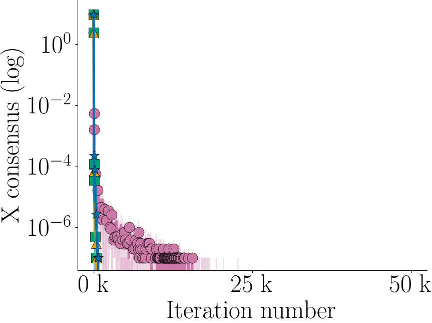
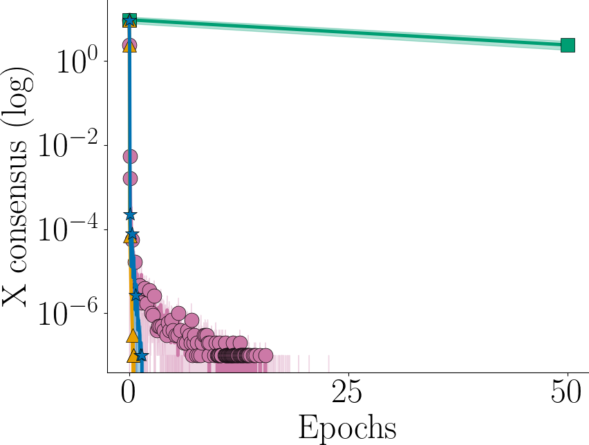
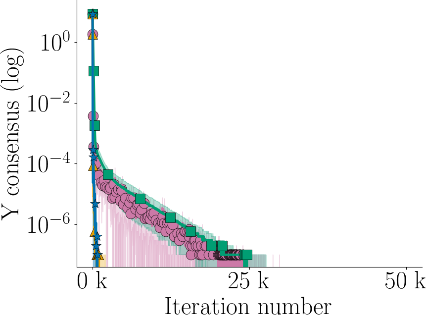
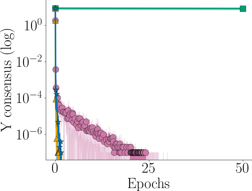
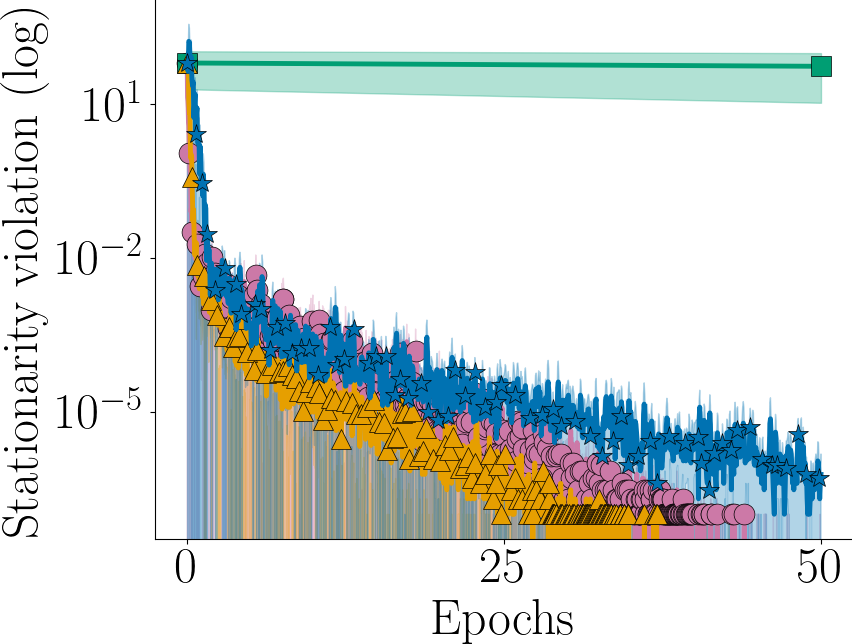
Figure 1: Experiment results for the PL game (15). The left column shows results in terms of algorithm iterations, while the right shows results in terms of data passes.

6.2 Robust Machine Learning

We consider two decentralized robust machine learning problems: non-convex linear regression with tabular data and neural network training with image data. We let each agent $i=1,\dots,m$ contain a dataset of points and labels denoted $\{(\mathbf{a}_{ij},b_{ij})\}_{j=1}^{n}$ where $b_{ij}$ is the class label of data point $\mathbf{a}_{ij}$. For these problems, $\mathbf{y}_{i}^{(*)}:=\arg\max_{\mathbf{y}_{i}}f_{i}(\mathbf{x},\mathbf{y}_{i})$ is not easily computable; as a proxy, we report the stationarity violation as

$$\|\frac{1}{m}\sum_{i=1}^{m}\nabla f_{i}(\bar{\mathbf{x}},\bar{\mathbf{y}})\|_{2}^{2}+\|\mathbf{X}_{\perp}\|_{F}^{2}+\|\mathbf{Y}_{\perp}\|_{F}^{2}.$$ (18)

6.2.1 Robust Non-convex Linear Regression

We consider training a robust version of the non-convex linear regression classifier from [36]. Local agent functions are given by

$$f_{i}(\mathbf{x}_{i},\mathbf{y}_{i})=\frac{1}{n}\sum_{j=1}^{n}\ln\left(\frac{\left(b_{ij}-\mathbf{x}_{i}^{\top}(\mathbf{a}_{ij}+\mathbf{y}_{i})\right)^{2}}{2}+1\right)-\frac{\alpha}{2}\|\mathbf{y}_{i}\|_{2}^{2}$$ (19)

where $b_{ij}\in\{-1,+1\}$ and $\alpha>0$ is a penalty term which guarantees the problem is strongly-concave in $\mathbf{y}$; we choose $\alpha=1.0$ for these experiments. The $\mathbf{y}$ variable acts as a perturbation to the data, hence we seek to maximize the perturbation, while simultaneously minimizing the loss on the perturbed data. We compare across two datasets: a9a and ijcnn1, both of which can be downloaded from https://www.csie.ntu.edu.tw/cjlin/libsvmtools/datasets/. Each $\mathbf{a}_{ij}\in\mathbb{R}^{123}$ for a9a and $\mathbb{R}^{22}$ for ijcnn1. We run each method to 5,000 iterations and additionally plot results until 50 epochs have been completed by each method. Results are reported in Figure 2. The main bottle neck for other methods which prevent a low violation of (18) is either the consensus on $\{\mathbf{x}_{i}\}$ or $\{\mathbf{y}_{i}\}$; from this, we can conclude that our proposed method acheives consensus extremely well in practice.

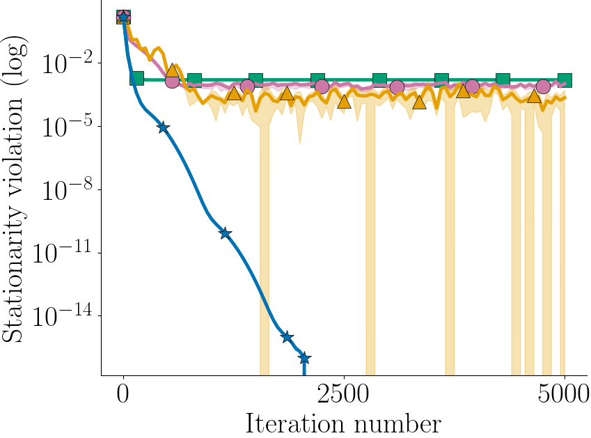
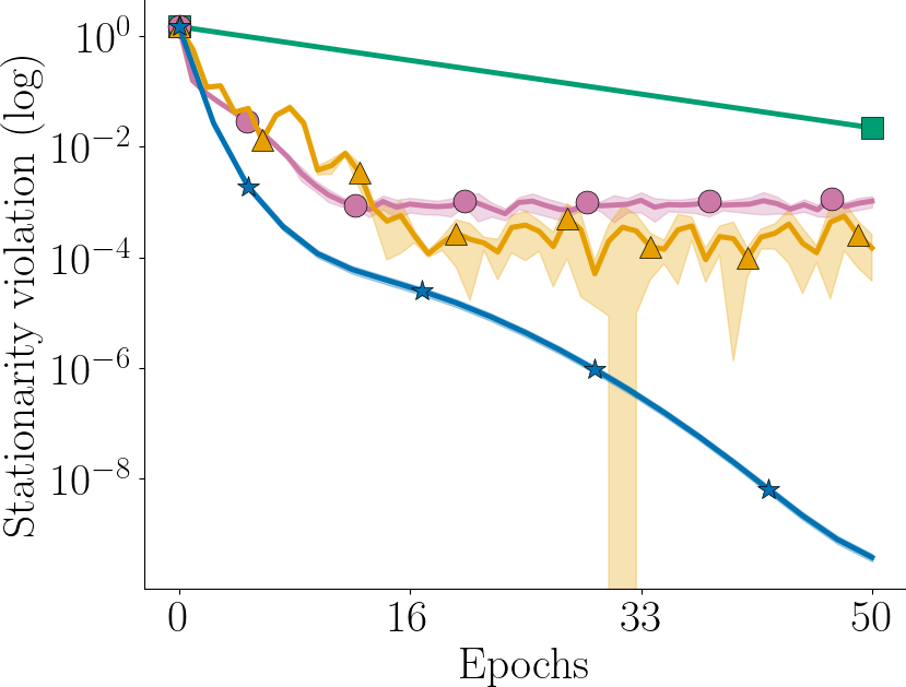
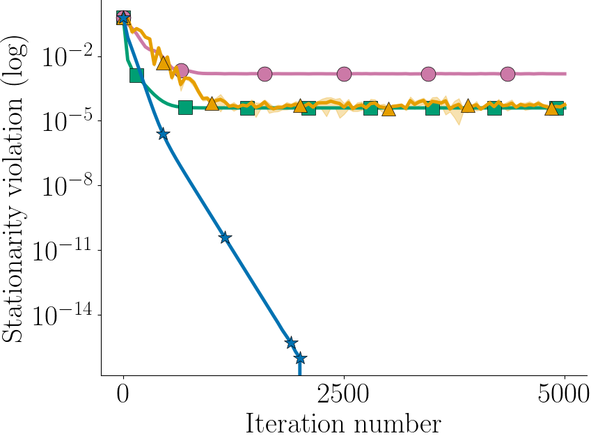
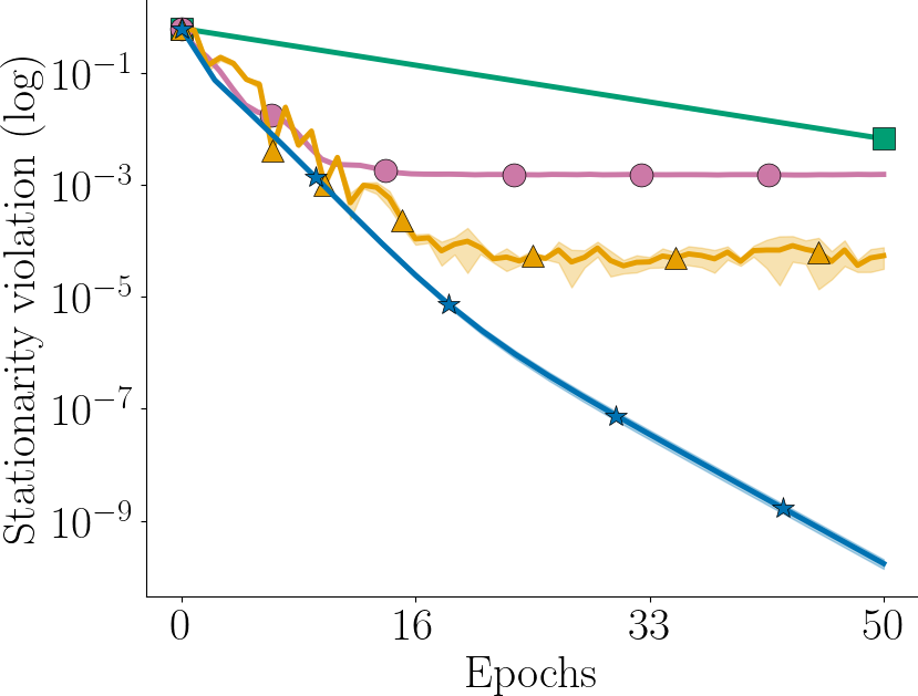
Figure 2: Experiment results for the robust non-convex linear regression model (19). The left column shows results in terms of algorithm iterations, while the right shows results in terms of data passes. The first row corresponds to the a9a dataset, while the second corresponds to the ijcnn1 dataset.

6.2.2 Robust Neural Network Training

We consider a slightly modified version of the robust neural network training problem from [8, 34]. Local agent functions are given by

$$f_{i}(\mathbf{x}_{i},\mathbf{y}_{i})=\frac{1}{n}\sum_{j=1}^{n}\ell\left(g_{\mathbf{x}_{i}}(\mathbf{a}_{ij}+\mathbf{y}_{i}),b_{ij}\right)-\frac{\alpha}{2}\|\mathbf{y}_{i}\|_{2}^{2}$$ (20)

where $g_{\mathbf{x}_{i}}$ is a neural network parameterized by $\mathbf{x}_{i}$, $\ell$ is the cross-entropy loss function, and $\alpha>0$ is a penalty term which guarantees the problem is strongly-concave in $\mathbf{y}$; we choose $\alpha=1.0$ for these experiments. Inspired by [8], we let $g_{\mathbf{x}_{i}}$ be a two-layer network (200 hidden units) with a tanh activation function, $\ell$ be the cross-entropy loss, and use the MNIST [16] dataset for training. We fix the mini-batch size for all methods to be 100 (besides GT/DA). For our proposed method, we set $q=100$ and let $S_{1}=7{,}500$. We run each algorithm to 50,000 iterations and additionally plot results until 500 epochs have been completed by each method. Results are shown in Figure 3. Our method has comparable performance to the compared stochastic methods and still outperforms the deterministic method in terms of data passes.

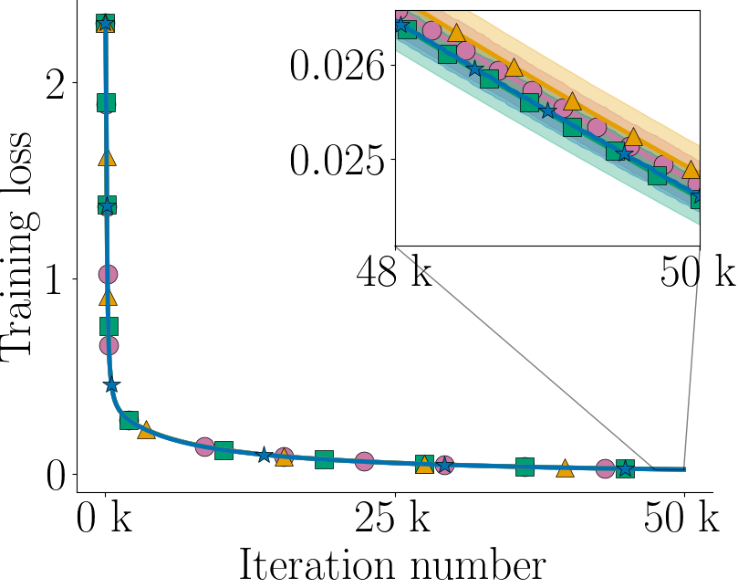
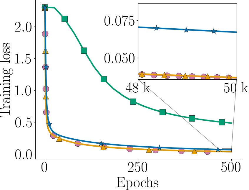
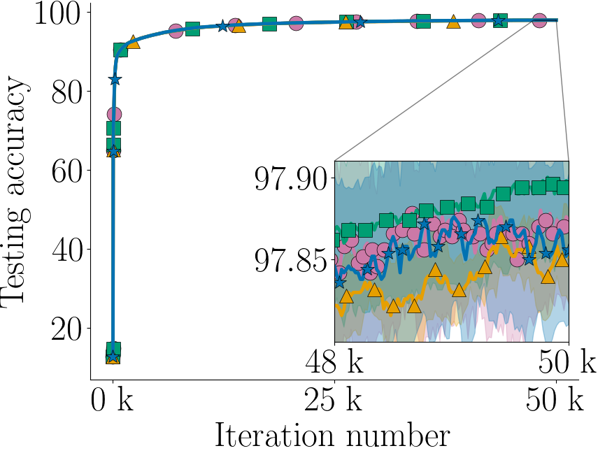
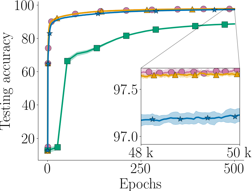
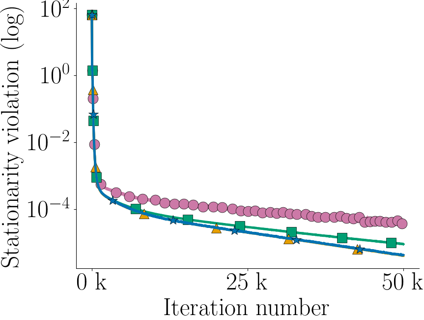
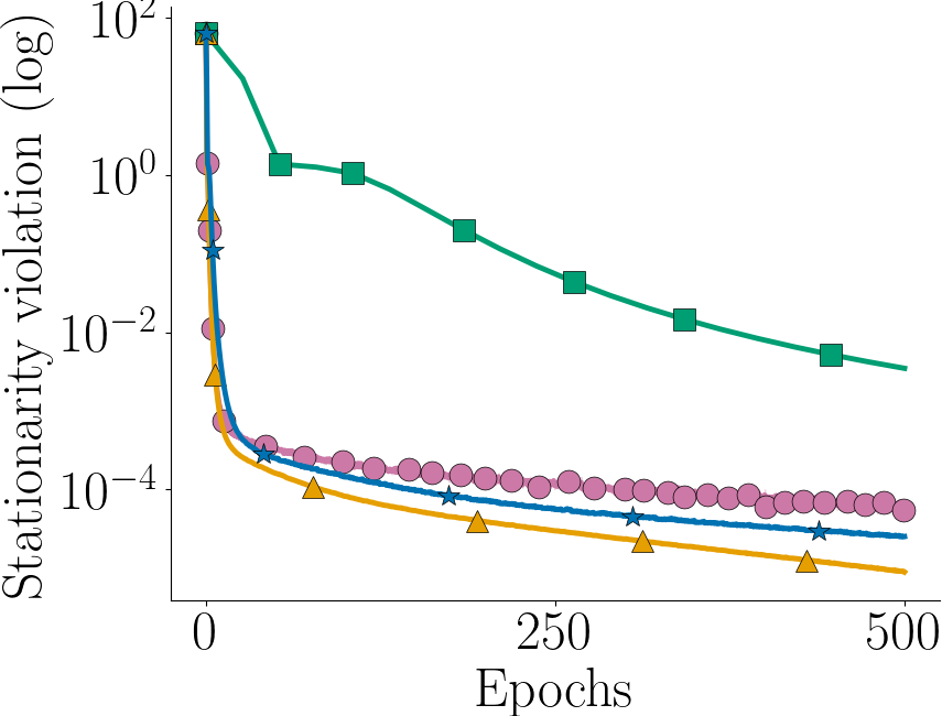
Figure 3: Experiment results for the robust neural network training problem (20). The left column shows results in terms of algorithm iterations, while the right shows results in terms of data passes.

7 Conclusion

In this work, we proposed a Decentralized Gradient Decent Ascent - Variance Reduction method, black, for solving the stochastic nonconvex strongly-concave minimax problem over a connected network of $M$ computing agents. Under the assumption that the computing agents only have access to stochastic first-order oracles, our method incorporates variance reduction and gradient tracking to jointly optimize the sample and communication complexities to be $\mathcal{O}\left(\epsilon^{-3}\right)$ and $\mathcal{O}\left(\epsilon^{-2}\right)$, respectively, for reaching an $\epsilon$-accurate solution. For the class of problems considered here, this is the first work which does not require multiple coordinated communications in each iteration to achieve these optimal complexities.

Appendix A Notation

To aid readability, we list the frequently used notation in the proof as follows:

• We defined $\Phi(\cdot)=\max_{\mathbf{y}}f(\cdot,\mathbf{y})$ and the condition number $\kappa$ in Definition 2.

• We defined $\mathbf{y}^{*}(\cdot)=\operatorname*{argmax}_{y}f(\cdot,\mathbf{y})$ in (8).

• We defined $\delta_{t}=\|\mathbf{y}^{*}(\bar{\mathbf{x}}^{t})-\bar{\mathbf{y}}^{t}\|^{2}$ in (13).

• The matrices and vector notations are defined in Definitions 4 and 5. The stochastic gradient estimate error $\{E^{t}\}$ and $\{\mathbf{e}^{t}_{i}\}$ are defined in (14).

• We use subscripts $x,y$ to represent the components of vectors or matrices, for example, $\mathbf{e}_{x,i}^{t}\triangleq\mathbf{v}_{x,i}^{t}-\nabla_{x}f_{i}(\mathbf{x}_{i}^{t},\mathbf{y}_{i}^{t})$ for $i\in[M]$.

Appendix B The General Proof Construction

In general, the proof of our main result Theorem 1 is based on the fundamental inequality:

$$\mathbf{E}[\Phi (\bar{\mathbf{x}}^{(n+1)q})]-\mathbf{E}[\Phi(\bar{\mathbf{x}}^{nq})]\leq\Theta(q\eta_{x}\sigma^{2}/S_{1})$$

$$-\sum_{t=nq}^{(n+1)q-1}\Big{(}\Theta(\eta_{x})\|\nabla\Phi(\bar{\mathbf{x}}^{t})\|^{2}-\Theta(\eta_{x}L^{2})\delta_{t}-\Theta(\frac{\eta_{x}L^{2}}{M})\|Z^{t}_{\perp}\|^{2}_{F}-\Theta(\frac{\eta_{x}\eta_{y}^{2}L^{2}}{M})\|D^{t}_{\perp}\|_{F}^{2}\Big{)}$$

which is shown in Lemma 7. From this inequality, we bound $\delta_{t}$, $\|Z^{t}_{\perp}\|_{F}^{2}$, and $\|D^{t}_{\perp}\|^{2}_{F}$ in Lemmas 8 and 11. To accomplish this, we also need to bound the error $\|E^{t}\|_{F}^{2}$ that is caused by the stochastic oracles and our variance reduction gradient estimator. The bound of $\|E^{t}\|$ is provided in Lemma 5, and is frequently used in other parts of the proof. After this, we invoke Lemmas 11 and 8 within Lemma 7, and then obtain the general convergence results of $\|\nabla\Phi(\bar{\mathbf{x}}^{t})\|$ in Theorem 3 through the following inequality:

$$\sum_{t=0}^{T-1}\mathbf{E}[\|\nabla\Phi(\bar{\mathbf{x}}^{t})\|^{2}]\leq\mathcal{O}\Big{(}\frac{1}{\eta_{x}}+\frac{L\kappa\delta_{0}}{\eta_{y}}+\frac{L^{2}\kappa^{2}\Lambda_{0}}{M}+T\cdot\frac{\kappa^{2}\sigma^{2}}{S_{1}}\Big{)}.$$ (21)

To achieve this concise bound, we also provide the parameter analysis in Appendix E to simplify the complicated terms in the proof. In the last, we provide the proper parameter choices and obtain the detailed sample complexity and communication complexity given certain parameter choices in Theorem 4 for running black. Before beginning the analysis, we restate a useful Lemma from the literature that is commonly employed in the convergence analysis of first-order algorithms.

Lemma 1 (Proposition 1 [6]).

Suppose Assumptions 1,  2, and 3 hold. Then $\Phi(\cdot):\mathbb{R}^{d}\rightarrow\mathbb{R}$ is $(\kappa+1)L$-smooth and $\nabla\Phi(\cdot)=f(\cdot,\mathbf{y}^{*}(\cdot))$. Moreover, $\mathbf{y}^{*}(\cdot):\mathbb{R}^{d}\rightarrow\mathbb{R}^{m}$ is $\kappa$-Lipschitz.

Appendix C Convergence Analysis

We begin by analyzing the measure of the dual suboptimality sequence $\{\delta_{t}\}$. It is important to note that many of the equations in this proof will be reused in other parts of the paper.

Lemma 2.

Suppose Assumptions 1, 2 and 6 hold. If $\eta_{y}\in(0,1/L]$, then the inequality

$$\delta_{t}\leq \Big{(}1-\frac{1}{4}\eta_{y}\mu+3\Big{(}\frac{4}{\eta_{y}\mu}-1\Big{)}\kappa^{2}\eta_{x}^{2}L^{2}\Big{)}\delta_{t-1}+\Big{(}\frac{4-\eta_{y}\mu}{4-2\eta_{y}\mu}\frac{2\eta_{y}}{\mu}+3\Big{(}\frac{4}{\eta_{y}\mu}-1\Big{)}\kappa^{2}\eta_{x}^{2}\Big{)}\frac{2L^{2}}{M}{\color[rgb]{0,0,0}\|Z^{t-1}_{\perp}\|^{2}_{F}}$$ (22)

$$+\frac{4-\eta_{y}\mu}{4-2\eta_{y}\mu}\frac{2\eta_{y}}{\mu}\frac{2}{M}\sum_{i=1}^{M}\|\mathbf{e}^{{\color[rgb]{0,0,0}t-1}}_{y,i}\|^{2}{\color[rgb]{0,0,0}+\Big{(}\frac{4}{\eta_{y}\mu}-1\Big{)}\kappa^{2}\eta_{x}^{2}\frac{6}{M}\sum_{i=1}^{M}\|\mathbf{e}^{t-1}_{x,i}\|^{2}}+3\Big{(}\frac{4}{\eta_{y}\mu}-1\Big{)}\kappa^{2}\eta_{x}^{2}\|\nabla\Phi(\bar{\mathbf{x}}^{t-1})\|^{2}$$

holds for all $t\geq 1$, where $\delta_{t}=\|{\mathbf{y}}^{*}(\bar{\mathbf{x}}^{t})-\bar{\mathbf{y}}^{t}\|^{2}$ is defined in (13).

Proof.

Using the facts $\bar{\mathbf{y}}^{t+1}=\bar{\mathbf{y}}^{t}+\eta_{y}\bar{\mathbf{d}}^{t}_{y}=\bar{\mathbf{y}}^{t}+\eta_{y}\bar{\mathbf{v}}^{t}_{y}$ and $\nabla_{y}f(\bar{\mathbf{x}}^{t},{\mathbf{y}}^{*}(\bar{\mathbf{x}}^{t}))=0$, we have that for any $a>0$,

$$\|{\mathbf{y}}^{*}(\bar{\mathbf{x}}^{t})-\bar{\mathbf{y}}^{t+1}\|^{2}=\|{\mathbf{y}}^{*}(\bar{\mathbf{x}}^{t})+\eta_{y}\nabla_{y}f(\bar{\mathbf{x}}^{t},{\mathbf{y}}^{*}(\bar{\mathbf{x}}^{t}))-\bar{\mathbf{y}}^{t}-\eta_{y}\bar{\mathbf{v}}^{t}\|^{2}$$ (23)

$$\leq (1+a)\|{\mathbf{y}}^{*}(\bar{\mathbf{x}}^{t})+\eta_{y}\nabla_{y}f(\bar{\mathbf{x}}^{t},{\mathbf{y}}^{*}(\bar{\mathbf{x}}^{t}))-\bar{\mathbf{y}}^{t}-\eta_{y}\nabla_{y}f(\bar{\mathbf{x}}^{t},\bar{\mathbf{y}}^{t})\|^{2}+(\textstyle 1+\frac{1}{a})\eta_{y}^{2}\|\nabla_{y}f(\bar{\mathbf{x}}^{t},\bar{\mathbf{y}}^{t})-\bar{\mathbf{v}}^{t}_{y}\|^{2}.$$

We bound the first term on the right hand side of (23) as follows:

$$\|{\mathbf{y}}^{*}(\bar{\mathbf{x}}^{t})+\eta_{y}\nabla_{y}f(\bar{\mathbf{x}}^{t},{\mathbf{y}}^{*}(\bar{\mathbf{x}}^{t}))-\bar{\mathbf{y}}^{t}-\eta_{y}{\color[rgb]{0,0,0}\nabla_{y}f(\bar{\mathbf{x}}^{t},\bar{\mathbf{y}}^{t})}\|^{2}$$ (24)

$$= \|{\mathbf{y}}^{*}(\bar{\mathbf{x}}^{t})-\bar{\mathbf{y}}^{t}\|^{2}+2\eta_{y}\left\langle{\mathbf{y}}^{*}(\bar{\mathbf{x}}^{t})-\bar{\mathbf{y}}^{t},\nabla_{y}f(\bar{\mathbf{x}}^{t},{\mathbf{y}}^{*}(\bar{\mathbf{x}}^{t}))-\nabla_{y}f(\bar{\mathbf{x}}^{t},\bar{\mathbf{y}}^{t})\right\rangle+\eta_{y}^{2}\|\nabla_{y}f(\bar{\mathbf{x}}^{t},{\mathbf{y}}^{*}(\bar{\mathbf{x}}^{t}))-\nabla_{y}f(\bar{\mathbf{x}}^{t},\bar{\mathbf{y}}^{t})\|^{2}$$

$$\leq \|{\mathbf{y}}^{*}(\bar{\mathbf{x}}^{t})-\bar{\mathbf{y}}^{t}\|^{2}+(2\eta_{y}-\eta_{y}^{2}L)\left\langle{\mathbf{y}}^{*}(\bar{\mathbf{x}}^{t})-\bar{\mathbf{y}}^{t},\nabla_{y}f(\bar{\mathbf{x}}^{t},{\mathbf{y}}^{*}(\bar{\mathbf{x}}^{t}))-\nabla_{y}f(\bar{\mathbf{x}}^{t},\bar{\mathbf{y}}^{t})\right\rangle$$

$$\leq (1-2\eta_{y}\mu+\eta_{y}^{2}\mu L){\color[rgb]{0,0,0}\|{\mathbf{y}}^{*}(\bar{\mathbf{x}}^{t})-\bar{\mathbf{y}}^{t}\|^{2}},$$

where the first inequality is by 1 and the concavity of $f(\mathbf{x},\cdot)$; the second inequality is by the strong concavity of $f(\mathbf{x},\cdot)$. Therefore, plugging (24) into (23), we have that for any $a>0$,

$$\|{\mathbf{y}}^{*}(\bar{\mathbf{x}}^{t})-\bar{\mathbf{y}}^{t+1}\|^{2}\leq (1+a)(1-2\eta_{y}\mu+\eta_{y}^{2}\mu L)\|{\mathbf{y}}^{*}(\bar{\mathbf{x}}^{t})-\bar{\mathbf{y}}^{t}\|^{2}+(1+\frac{1}{a})\eta_{y}^{2}\|\nabla_{y}f(\bar{\mathbf{x}}^{t},\bar{\mathbf{y}}^{t})-\bar{\mathbf{v}}^{t}_{y}\|^{2}$$ (25)

$$\leq (1+a)\left(1-\eta_{y}\mu\right)\delta_{t}+(1+\frac{1}{a})\eta_{y}^{2}\|\nabla_{y}f(\bar{\mathbf{x}}^{t},\bar{\mathbf{y}}^{t})-\bar{\mathbf{v}}^{t}_{y}\|^{2}$$

$$= (1-\frac{1}{2}\eta_{y}\mu)\delta_{t}+\left(\frac{2}{\eta_{y}\mu}-1\right)\eta_{y}^{2}\|\nabla_{y}f(\bar{\mathbf{x}}^{t},\bar{\mathbf{y}}^{t})-\bar{\mathbf{v}}^{t}_{y}\|^{2}$$

$$\leq \left(1-\frac{1}{2}\eta_{y}\mu\right)\delta_{t}+\frac{2\eta_{y}}{\mu}\|\nabla_{y}f(\bar{\mathbf{x}}^{t},\bar{\mathbf{y}}^{t})-\bar{\mathbf{v}}^{t}_{y}\|^{2}$$

where in the second inequality we use $\eta_{y}\in(0,1/L]$, and in the equality we set $a=\frac{\eta_{y}\mu}{2-2\eta_{y}\mu}$. Moreover, we can bound $\|\bar{\mathbf{v}}^{t}_{y}-\nabla_{y}f(\bar{\mathbf{x}}^{t},\bar{\mathbf{y}}^{t})\|^{2}$ as follows:

$$\|\nabla_{y}f(\bar{\mathbf{x}}^{t},\bar{\mathbf{y}}^{t})-\bar{\mathbf{v}}^{t}_{y}\|^{2}= \left\|\nabla_{y}f(\bar{\mathbf{x}}^{t},\bar{\mathbf{y}}^{t})-\frac{1}{M}\sum_{i=1}^{M}\nabla_{y}f_{i}(\mathbf{x}^{t}_{i},\mathbf{y}^{t}_{i})+\frac{1}{M}\sum_{i=1}^{M}\nabla_{y}f_{i}(\mathbf{x}^{t}_{i},\mathbf{y}^{t}_{i})-\bar{\mathbf{v}}^{t}_{y}\right\|^{2}$$ (26)

$$\leq 2\left\|{\color[rgb]{0,0,0}\frac{1}{M}\sum_{i=1}^{M}}\nabla_{y}{\color[rgb]{0,0,0}f_{i}}(\bar{\mathbf{x}}^{t},\bar{\mathbf{y}}^{t})-\frac{1}{M}\sum_{i=1}^{M}\nabla_{y}f_{i}(\mathbf{x}^{t}_{i},\mathbf{y}^{t}_{i})\right\|^{2}+2\left\|\frac{1}{M}\sum_{i=1}^{M}\nabla_{y}f_{i}(\mathbf{x}^{t}_{i},\mathbf{y}^{t}_{i})-\frac{1}{M}\sum_{i=1}^{M}\mathbf{v}^{t}_{y,i}\right\|^{2}$$

$$\leq \frac{2}{M}\sum_{i=1}^{M}\Big{(}\|\nabla_{y}{\color[rgb]{0,0,0}f_{i}}(\bar{\mathbf{x}}^{t},\bar{\mathbf{y}}^{t})-\nabla_{y}f_{i}(\mathbf{x}^{t}_{i},\mathbf{y}^{t}_{i})\|^{2}+\|\nabla_{y}f_{i}(\mathbf{x}^{t}_{i},\mathbf{y}^{t}_{i})-\mathbf{v}^{t}_{y,i}\|^{2}\Big{)}$$

$$\leq \frac{2L^{2}}{M}(\|X^{t}_{\perp}\|^{2}_{F}+\|Y^{t}_{\perp}\|^{2}_{F})+\frac{2}{M}\sum_{i=1}^{M}\|\mathbf{e}^{t}_{y,i}\|^{2}$$

where the last inequality follows from 1, and $X_{\perp}$, $Y_{\perp}$, and $\mathbf{e}^{t}_{y,i}$ are defined in Appendix A. Then, plugging (26) into (25), we have

$$\|{\mathbf{y}}^{*}(\bar{\mathbf{x}}^{t})-\bar{\mathbf{y}}^{t+1}\|^{2}\leq \left(1-\frac{1}{2}\eta_{y}\mu\right)\delta_{t}+\frac{2\eta_{y}}{\mu}\Big{(}\frac{2L^{2}}{M}(\|X^{t}_{\perp}\|^{2}_{F}+\|Y^{t}_{\perp}\|^{2}_{F})+\frac{2}{M}\sum_{i=1}^{M}\|\mathbf{e}^{t}_{y,i}\|^{2}\Big{)}.$$ (27)

Now, we are ready to show a proper bound for $\delta_{t}$ for all $t\geq 1$. Indeed, for $\forall a>0$, we have

$$\delta_{t}=\|{\mathbf{y}}^{*}(\bar{\mathbf{x}}^{t})-{\mathbf{y}}^{*}(\bar{\mathbf{x}}^{t-1})+{\mathbf{y}}^{*}(\bar{\mathbf{x}}^{t-1})-\bar{\mathbf{y}}^{t}\|^{2}$$ (28)

$$\leq (1+a)\|{\mathbf{y}}^{*}(\bar{\mathbf{x}}^{t-1})-\bar{\mathbf{y}}^{t}\|^{2}+\left(1+\frac{1}{a}\right)\|{\mathbf{y}}^{*}(\bar{\mathbf{x}}^{t})-{\mathbf{y}}^{*}(\bar{\mathbf{x}}^{t-1})\|^{2}$$

$$\leq (1+a)\|{\mathbf{y}}^{*}(\bar{\mathbf{x}}^{t-1})-\bar{\mathbf{y}}^{t}\|^{2}+\left(1+\frac{1}{a}\right)\kappa^{2}\|\bar{\mathbf{x}}^{t}-\bar{\mathbf{x}}^{t-1}\|^{2}$$

$$\leq (1+a)\left(\Big{(}1-\frac{1}{2}\eta_{y}\mu\Big{)}\delta_{t-1}+\frac{2\eta_{y}}{\mu}\frac{2L^{2}}{M}(\|X^{t-1}_{\perp}\|^{2}_{F}+\|Y^{t-1}_{\perp}\|^{2}_{F})+\frac{2\eta_{y}}{\mu}\frac{2}{M}\sum_{i=1}^{M}\|\mathbf{e}^{t-1}_{y,i}\|^{2}\right)+\left(1+\frac{1}{a}\right)\kappa^{2}\|\bar{\mathbf{x}}^{t}-\bar{\mathbf{x}}^{t-1}\|^{2},$$

where the second inequality is by Lemma 1; the last inequality is by (27). Next, letting $a=\frac{\eta_{y}\mu}{4-2\eta_{y}\mu}$ and using the fact $\bar{\mathbf{x}}^{t}=\bar{\mathbf{x}}^{t-1}-\eta_{x}\bar{\mathbf{v}}^{t-1}$, we obtain

$$\delta_{t}\leq \left(1-\frac{1}{4}\eta_{y}\mu\right)\delta_{t-1}+\frac{4-\eta_{y}\mu}{4-2\eta_{y}\mu}\frac{2\eta_{y}}{\mu}\frac{2L^{2}}{M}\left(\|X^{t-1}_{\perp}\|^{2}_{F}+\|Y^{t-1}_{\perp}\|^{2}_{F}\right)$$ (29)

$$+\frac{4-\eta_{y}\mu}{4-2\eta_{y}\mu}\frac{2\eta_{y}}{\mu}\frac{2}{M}\sum_{i=1}^{M}\|\mathbf{e}^{t-1}_{y,i}\|^{2}+\left(\frac{4}{\eta_{y}\mu}-1\right)\kappa^{2}\eta_{x}^{2}\|\bar{\mathbf{v}}^{t-1}_{x}\|^{2}.$$

In the following part, we first provide an upper bound on $\|\bar{\mathbf{v}}^{t}_{x}\|^{2}$, and then use it within (29). Indeed, we have

$$\|\bar{\mathbf{v}}^{t}_{x}\|^{2}= \|\bar{\mathbf{v}}^{t}_{x}-\nabla_{x}f(\bar{\mathbf{x}}^{t},\bar{\mathbf{y}}^{t})+\nabla_{x}f(\bar{\mathbf{x}}^{t},\bar{\mathbf{y}}^{t})-\nabla\Phi(\bar{\mathbf{x}}^{t})+\nabla\Phi(\bar{\mathbf{x}}^{t})\|^{2}$$ (30)

$$\leq 3\|\bar{\mathbf{v}}^{t}_{x}-\nabla_{x}f(\bar{\mathbf{x}}^{t},\bar{\mathbf{y}}^{t})\|^{2}+3\|\nabla_{x}f(\bar{\mathbf{x}}^{t},\bar{\mathbf{y}}^{t})-\nabla\Phi(\bar{\mathbf{x}}^{t})\|^{2}+3\|\nabla\Phi(\bar{\mathbf{x}}^{t})\|^{2}$$

$$\leq 3\|\bar{\mathbf{v}}^{t}_{x}-\nabla_{x}f(\bar{\mathbf{x}}^{t},\bar{\mathbf{y}}^{t})\|^{2}+3L^{2}\delta_{t}+3\|\nabla\Phi(\bar{\mathbf{x}}^{t})\|^{2},$$

where the last inequality is by 1 and $\Phi(\mathbf{x})=\max_{\mathbf{y}\in\mathbb{R}^{m}}f(\mathbf{x},\mathbf{y})$ is defined in Lemma 1; specifically, the definition of $\Phi(\mathbf{x})$ implies $\nabla\Phi(\bar{\mathbf{x}}^{t})=\nabla_{x}f(\bar{\mathbf{x}}^{t},\mathbf{y}^{*}(\bar{\mathbf{x}}^{t}))$. Furthermore, similar to Equation 26, we also have

$$\|\nabla_{x}f(\bar{\mathbf{x}}^{t},\bar{\mathbf{y}}^{t})-\bar{\mathbf{v}}^{t}_{x}\|^{2}\leq\frac{2L^{2}}{M}(\|X^{t}_{\perp}\|^{2}_{F}+\|Y^{t}_{\perp}\|^{2}_{F})+\frac{2}{M}\sum_{i=1}^{M}\|\mathbf{e}^{t}_{x,i}\|^{2}.$$ (31)

If we use (31) within (30), it follows that

$$\|\bar{\mathbf{v}}^{t}_{x}\|^{2}\leq \frac{6L^{2}}{M}(\|X^{t}_{\perp}\|^{2}_{F}+\|Y^{t}_{\perp}\|^{2}_{F})+\frac{6}{M}\sum_{i=1}^{M}\|\mathbf{e}^{t}_{x,i}\|^{2}+3L^{2}\delta_{t}+3\|\nabla\Phi(\bar{\mathbf{x}}^{t})\|^{2}.$$ (32)

Next, using (32) within (29) gives

$$\delta_{t}\leq \Big{(}1-\frac{1}{4}\eta_{y}\mu\Big{)}\delta_{t-1}+\frac{4-\eta_{y}\mu}{4-2\eta_{y}\mu}\frac{2\eta_{y}}{\mu}\frac{2L^{2}}{M}(\|X^{t-1}_{\perp}\|^{2}_{F}+\|Y^{t-1}_{\perp}\|^{2}_{F})+\frac{4-\eta_{y}\mu}{4-2\eta_{y}\mu}\frac{2\eta_{y}}{\mu}\frac{2}{M}\sum_{i=1}^{M}\|\mathbf{e}^{t-1}_{y,i}\|^{2}$$ (33)

$$+\Big{(}\frac{4}{\eta_{y}\mu}-1\Big{)}\kappa^{2}\eta_{x}^{2}\Big{(}\frac{6L^{2}}{M}(\|X^{t-1}_{\perp}\|^{2}_{F}+\|Y^{t-1}_{\perp}\|^{2}_{F})+\frac{6}{M}\sum_{i=1}^{M}\|\mathbf{e}^{t-1}_{x,i}\|^{2}+3L^{2}\delta_{t-1}+3\|\nabla\Phi(\bar{\mathbf{x}}^{t-1})\|^{2}\Big{)}$$

$$= \Big{(}1-\frac{1}{4}\eta_{y}\mu+3\Big{(}\frac{4}{\eta_{y}\mu}-1\Big{)}\kappa^{2}\eta_{x}^{2}L^{2}\Big{)}\delta_{t-1}+\Big{(}\frac{4-\eta_{y}\mu}{4-2\eta_{y}\mu}\frac{2\eta_{y}}{\mu}+3\Big{(}\frac{4}{\eta_{y}\mu}-1\Big{)}\kappa^{2}\eta_{x}^{2}\Big{)}\frac{2L^{2}}{M}(\|X^{{\color[rgb]{0,0,0}t-1}}_{\perp}\|^{2}_{F}+\|Y^{{\color[rgb]{0,0,0}t-1}}_{\perp}\|^{2}_{F})$$

$$+\frac{4-\eta_{y}\mu}{4-2\eta_{y}\mu}\frac{2\eta_{y}}{\mu}\frac{2}{M}\sum_{i=1}^{M}\|\mathbf{e}^{{\color[rgb]{0,0,0}t-1}}_{y,i}\|^{2}{\color[rgb]{0,0,0}+\Big{(}\frac{4}{\eta_{y}\mu}-1\Big{)}\kappa^{2}\eta_{x}^{2}\frac{6}{M}\sum_{i=1}^{M}\|\mathbf{e}^{t-1}_{x,i}\|^{2}}+3\Big{(}\frac{4}{\eta_{y}\mu}-1\Big{)}\kappa^{2}\eta_{x}^{2}\|\nabla\Phi(\bar{\mathbf{x}}^{t-1})\|^{2}.$$

Now using the fact $\|Z^{t}_{\perp}\|^{2}_{F}=\|X^{t}_{\perp}\|^{2}_{F}+\|Y^{t}_{\perp}\|^{2}_{F}$ completes the proof. ∎

We temporarily stop the analysis of $\delta_{t}$ here. In section Section C.3, we will continue to investigate the bound of $\delta_{t}$. The reason why we presented this part of the proof first is that it includes many technical equations that are used in other parts of the analysis. Next, we will proceed to analyze the error of the stochastic gradient oracles $\|E^{t}\|^{2}_{F}$.

C.1 Bound of Stochastic Gradient Estimate

In this section, we establish a suitable upper bound for $\mathbf{E}[\|E^{t}\|^{2}_{F}]$. The bound will be frequently used in the analysis of $\{\nabla\Phi(\bar{\mathbf{x}}^{t}),\delta_{t},\|Z^{t}_{\perp}\|^{2}_{F},\|D^{t}_{\perp}\|^{2}_{F}\}$.

Lemma 3.

Suppose Assumptions 2, 4, 5 and 6 hold. Given $q\geq 1$, the inequality

$$\mathbf{E}[\|\mathbf{e}^{t}_{i}\|^{2}]\leq \mathbf{E}[\|\mathbf{e}^{t-1}_{i}\|^{2}]+\frac{L^{2}}{S_{2}}\mathbf{E}[\|\mathbf{z}^{t}_{i}-\mathbf{z}^{t-1}_{i}\|^{2}],\quad{\color[rgb]{0,0,0}\forall~{}i\in[M]}$$ (34)

holds for all $t\geq 1$ such that $\rm{mod}(t,q)\neq 0$. Moreover, if $\rm{mod}(t,q)=0$, then $\mathbf{E}[\|\mathbf{e}^{t}_{i}\|^{2}]\leq\frac{\sigma^{2}}{S_{1}}$.

Proof.

Recall that $\mathbf{e}_{i}^{t}=\mathbf{v}_{i}^{t}-\nabla f_{i}(\mathbf{x}_{i}^{t},\mathbf{y}_{i}^{t})$ for $i=1,\ldots,M$ and $\mathbf{v}_{i}^{t}$ is defined in Definition 4. Thus, Given $i\in[M]$ and $t\geq 1$ such that $\rm{mod}(t,q)>0$, it follows from the definition of $\mathbf{v}^{t}_{i}$ and $\mathbf{e}^{t}_{i}$ that

$$\mathbf{E}\left[\left\|\|\mathbf{e}^{t}_{i}\|^{2}]=\right.\right. \mathbf{E}\Bigg{[}\Bigg{\|}\frac{1}{|{\color[rgb]{0,0,0}\mathcal{B}_{i}^{t}}|}\sum_{\xi\in{\color[rgb]{0,0,0}\mathcal{B}_{i}^{t}}}\Big{(}{\color[rgb]{0,0,0}\tilde{\nabla}f_{i}}(\mathbf{x}^{t}_{i},\mathbf{y}^{t}_{i};\xi)-{\color[rgb]{0,0,0}\tilde{\nabla}f_{i}}(\mathbf{x}^{t-1}_{i},\mathbf{y}^{t-1}_{i};\xi)\Big{)}+\mathbf{v}^{t-1}_{i}-\nabla f_{i}(\mathbf{x}^{t}_{i},\mathbf{y}^{t}_{i}))\Bigg{\|}^{2}\Bigg{]}$$ (35)

$$= \mathbf{E}\left[\left\|\frac{1}{|{\color[rgb]{0,0,0}\mathcal{B}_{i}^{t}}|}\sum_{\xi\in{\color[rgb]{0,0,0}\mathcal{B}_{i}^{t}}}\Big{(}{\color[rgb]{0,0,0}\tilde{\nabla}f_{i}}(\mathbf{x}^{t}_{i},\mathbf{y}^{t}_{i};\xi)-{\color[rgb]{0,0,0}\tilde{\nabla}f_{i}}(\mathbf{x}^{t-1}_{i},\mathbf{y}^{t-1}_{i};\xi)\Big{)}+\mathbf{e}^{t-1}_{i}-\nabla f_{i}(\mathbf{x}^{t}_{i},\mathbf{y}^{t}_{i})+\nabla f_{i}(\mathbf{x}^{t-1}_{i},\mathbf{y}^{t-1}_{i})\right\|^{2}\right]$$

$$= \mathbf{E}[\|\mathbf{e}^{t-1}_{i}\|^{2}]+\mathbf{E}\left[\left\|\frac{1}{|{\color[rgb]{0,0,0}\mathcal{B}_{i}^{t}}|}\sum_{\xi\in{\color[rgb]{0,0,0}\mathcal{B}_{i}^{t}}}\Big{(}{\color[rgb]{0,0,0}\tilde{\nabla}f_{i}}(\mathbf{x}^{t}_{i},\mathbf{y}^{t}_{i};\xi)-{\color[rgb]{0,0,0}\tilde{\nabla}f_{i}}(\mathbf{x}^{t-1}_{i},\mathbf{y}^{t-1}_{i};\xi)\Big{)}-\nabla f_{i}(\mathbf{x}^{t}_{i},\mathbf{y}^{t}_{i})+\nabla f_{i}(\mathbf{x}^{t-1}_{i},\mathbf{y}^{t-1}_{i})\right\|^{2}\right]$$

$$= \mathbf{E}[\|\mathbf{e}^{t-1}_{i}\|^{2}]+\frac{1}{|{\color[rgb]{0,0,0}\mathcal{B}_{i}^{t}}|^{2}}\sum_{\xi\in{\color[rgb]{0,0,0}\mathcal{B}_{i}^{t}}}\mathbf{E}\left[\|{\color[rgb]{0,0,0}\tilde{\nabla}f_{i}}(\mathbf{x}^{t}_{i},\mathbf{y}^{t}_{i};\xi)-{\color[rgb]{0,0,0}\tilde{\nabla}f_{i}}(\mathbf{x}^{t-1}_{i},\mathbf{y}^{t-1}_{i};\xi)-\nabla f_{i}(\mathbf{x}^{t}_{i},\mathbf{y}^{t}_{i})+\nabla f_{i}(\mathbf{x}^{t-1}_{i},\mathbf{y}^{t-1}_{i})\|^{2}\right].$$

The last two equalities above follow from the unbiasedness of the stochastic oracle in Assumption 4 and the independence of the elements in ${\color[rgb]{0,0,0}\mathcal{B}_{i}^{t}}$, which implies

$$\mathbf{E}[{\color[rgb]{0,0,0}\tilde{\nabla}f_{i}}(\mathbf{x}^{t}_{i},\mathbf{y}^{t}_{i};\xi)-{\color[rgb]{0,0,0}\tilde{\nabla}f_{i}}(\mathbf{x}^{t-1}_{i},\mathbf{y}^{t-1}_{i};\xi)-\nabla f_{i}(\mathbf{x}^{t}_{i},\mathbf{y}^{t}_{i})+\nabla f_{i}(\mathbf{x}^{t-1}_{i},\mathbf{y}^{t-1}_{i})]=0,\;\forall\xi\in{\color[rgb]{0,0,0}\mathcal{B}_{i}^{t}}.$$

Furthermore, since for any given random variable $\zeta$ with the finite second order moment, $\mathbf{E}[\|\zeta-\mathbf{E}[\zeta]\|^{2}]\leq\mathbf{E}[\|\zeta\|^{2}]$ holds, invoking this inequality for $\zeta={\color[rgb]{0,0,0}\tilde{\nabla}f_{i}}(\mathbf{x}^{t}_{i},\mathbf{y}^{t}_{i};\xi)-{\color[rgb]{0,0,0}\tilde{\nabla}f_{i}}(\mathbf{x}^{t-1}_{i},\mathbf{y}^{t-1}_{i};\xi)$, (35) implies that

$$\mathbf{E}[\|\mathbf{e}^{t}_{i}\|^{2}]\leq \mathbf{E}[\|\mathbf{e}^{t-1}_{i}\|^{2}]+\frac{1}{|{\color[rgb]{0,0,0}\mathcal{B}_{i}^{t}}|^{2}}\sum_{\xi\in{\color[rgb]{0,0,0}\mathcal{B}_{i}^{t}}}\mathbf{E}[\|{\color[rgb]{0,0,0}\tilde{\nabla}f_{i}}(\mathbf{x}^{t}_{i},\mathbf{y}^{t}_{i};\xi)-{\color[rgb]{0,0,0}\tilde{\nabla}f_{i}}(\mathbf{x}^{t-1}_{i},\mathbf{y}^{t-1}_{i};\xi)\|^{2}]$$ (36)

$$\leq \mathbf{E}[\|\mathbf{e}^{t-1}_{i}\|^{2}]+\frac{L^{2}}{|{\color[rgb]{0,0,0}\mathcal{B}_{i}^{t}}|}\mathbf{E}[\|\mathbf{x}^{t}_{i}-\mathbf{x}^{t-1}_{i}\|^{2}+\|\mathbf{y}^{t}_{i}-\mathbf{y}^{t-1}_{i}\|^{2}]$$

$$= \mathbf{E}[\|\mathbf{e}^{t-1}_{i}\|^{2}]+\frac{L^{2}}{|{\color[rgb]{0,0,0}\mathcal{B}_{i}^{t}}|}\mathbf{E}[\|\mathbf{z}^{t}_{i}-\mathbf{z}^{t-1}_{i}\|^{2}],$$

where the last inequality follows from 5. Since for $\rm{mod}(t,q)>0$ we set $|{\color[rgb]{0,0,0}\mathcal{B}_{i}^{t}}|=S_{2}$ for all $i\in[M]$, (34) follows immediately.

On the other hand, given $i\in[M]$, when $\rm{mod}(t,q)=0$, it directly follows from the definition of $\mathbf{e}^{t}_{i}$ and Assumption 4 that $\mathbf{E}[\|\mathbf{e}^{t}_{i}\|^{2}]\leq\frac{\sigma^{2}}{S_{1}}$, which completes the proof. ∎

Lemma 4.

Suppose Assumptions 2, 4, 5 and 6 hold, and $\eta_{x}\leq\eta_{y}$, then the inequality

$${\color[rgb]{0,0,0}\mathbf{E}[}\|Z^{t+1}-Z^{t}\|^{2}_{F}{\color[rgb]{0,0,0}]}\leq\frac{S_{2}}{L^{2}}\Delta_{t}+{\color[rgb]{0,0,0}24\eta_{y}^{2}}\mathbf{E}[\|E^{t}\|_{F}^{2}]$$ (37)

holds for all $t\geq 0$, where we define $E^{t}=[{\mathbf{e}^{t}_{1}},\mathbf{e}^{t}_{2},...,\mathbf{e}^{t}_{M}]^{\top}$, and

$$\Delta_{t}=\frac{L^{2}}{S_{2}}\mathbf{E}\Big{[}\Big{(}{\color[rgb]{0,0,0}8}+{\color[rgb]{0,0,0}40\eta_{y}^{2}L^{2}}\Big{)}\|Z^{t}_{\perp}\|^{2}_{F}+4\eta_{y}^{2}\|D^{t}_{\perp}\|^{2}_{F}+{\color[rgb]{0,0,0}20\eta_{y}^{2}L^{2}M\delta_{t}}+12M\eta_{x}^{2}\|\nabla\Phi(\bar{\mathbf{x}}^{t})\|^{2}\Big{]}.$$ (38)

Proof.

From the update in Algorithm 1 and 6, we have

$$\|X^{t+1}-X^{t}\|_{F}^{2}=\|WX^{t}-X^{t}-\eta_{x}D^{t}_{x}\|^{2}_{F}=\|(W-I)(X^{t}-\bar{X}^{t})-\eta_{x}D^{t}_{x}\|^{2}$$

$$\leq 2\|(W-I)X^{t}_{\perp}\|_{F}^{2}+2\eta_{x}^{2}\|D^{t}_{x}\|^{2}_{F}\leq{\color[rgb]{0,0,0}8}\|X^{t}_{\perp}\|_{F}^{2}+2\eta_{x}^{2}\|D^{t}_{x}\|^{2}_{F}.$$

Moreover, by Young’s inequality and the fact that $D^{t}_{x}=\bar{D}^{t}_{x}+D^{t}_{x\perp}$ and $\bar{D}^{t}_{x}=\bar{V}^{t}_{x}$, we have

$$\|X^{t+1}-X^{t}\|_{F}^{2}\leq{\color[rgb]{0,0,0}8}\|X^{t}_{\perp}\|_{F}^{2}+4\eta_{x}^{2}\|\bar{D}^{t}_{x}\|^{2}_{F}+4\eta_{x}^{2}\|D^{t}_{x\perp}\|^{2}_{F}{\color[rgb]{0,0,0}=}{\color[rgb]{0,0,0}8}\|X^{t}_{\perp}\|_{F}^{2}+4\eta_{x}^{2}\|\bar{V}^{t}_{x}\|^{2}_{F}+4\eta_{x}^{2}\|D^{t}_{x\perp}\|^{2}_{F}.$$ (39)

Similarly, we have

$$\|Y^{t+1}-Y^{t}\|_{F}^{2}\leq{\color[rgb]{0,0,0}8}\|Y^{t}_{\perp}\|_{F}^{2}+4\eta_{y}^{2}\|\bar{V}^{t}_{y}\|^{2}_{F}+4\eta_{y}^{2}\|D^{t}_{y\perp}\|^{2}_{F}.$$ (40)

Therefore, combining Equations 39 and 40, we have

$$\|Z^{t+1}-Z^{t}\|^{2}_{F}=\|X^{t+1}-X^{t}\|_{F}^{2}+\|Y^{t+1}-Y^{t}\|_{F}^{2}$$ (41)

$$\leq {\color[rgb]{0,0,0}8}\|X^{t}_{\perp}\|_{F}^{2}+4\eta_{x}^{2}\|D^{t}_{x\perp}\|^{2}_{F}+{\color[rgb]{0,0,0}8}\|Y^{t}_{\perp}\|_{F}^{2}+4\eta_{y}^{2}\|D^{t}_{y\perp}\|^{2}_{F}+4\eta_{x}^{2}\|\bar{V}^{t}_{x}\|^{2}_{F}+4\eta_{y}^{2}\|\bar{V}^{t}_{y}\|^{2}_{F}$$

$$\leq {\color[rgb]{0,0,0}8}\|Z^{t}_{\perp}\|_{F}^{2}+4\eta_{y}^{2}\|D^{t}_{\perp}\|^{2}_{F}+4\eta_{x}^{2}\|\bar{V}^{t}_{x}\|^{2}_{F}+4\eta_{y}^{2}\|\bar{V}^{t}_{y}\|^{2}_{F},$$

where we use the condition $\eta_{x}\leq\eta_{y}$ in the last inequality. Next, we will bound $\|\bar{V}^{t}_{x}\|^{2}_{F}$ and $\|\bar{V}^{t}_{y}\|^{2}_{F}$ separately. Specifically, it follows from (32) that

$$\|\bar{V}^{t}_{x}\|_{F}^{2}\leq 6L^{2}\|Z^{t}_{\perp}\|^{2}_{F}+6\sum_{i=1}^{M}\|\mathbf{e}^{t}_{x,i}\|^{2}+3ML^{2}\delta_{t}+3M\|\nabla\Phi(\bar{\mathbf{x}}^{t})\|^{2}.$$ (42)

On the other hand, we can bound $\|\bar{V}^{t}_{y}\|_{F}^{2}$ as follows

$$\|\bar{V}^{t}_{y}\|_{F}^{2}=M\|\bar{\mathbf{v}}^{t}\|^{2}$$ (43)

$$= M\|\bar{\mathbf{v}}^{t}-\nabla_{y}f(\bar{\mathbf{x}}^{t},\bar{\mathbf{y}}^{t})+\nabla_{y}f(\bar{\mathbf{x}}^{t},\bar{\mathbf{y}}^{t})-\nabla_{y}f(\bar{\mathbf{x}}^{t},\mathbf{y}_{*}(\bar{\mathbf{x}}^{t}))\|^{2}$$

$$\leq 2M\Big{(}\|\bar{\mathbf{v}}^{t}-\nabla_{y}f(\bar{\mathbf{x}}^{t},\bar{\mathbf{y}}^{t})\|^{2}+\|\nabla_{y}f(\bar{\mathbf{x}}^{t},\bar{\mathbf{y}}^{t})-\nabla_{y}f(\bar{\mathbf{x}}^{t},\mathbf{y}_{*}(\bar{\mathbf{x}}^{t}))\|^{2}\Big{)}$$

$$\leq 2L^{2}M\delta_{t}+4L^{2}\|Z^{t}_{\perp}\|^{2}+4\sum_{i=1}^{M}\|\mathbf{e}^{t}_{y,i}\|^{2}$$

where the last inequality follows from Equation 26 and 1. Therefore, if we use Equations 42 and 43 within Equation 41 and then use the condition $\eta_{x}\leq\eta_{y}$, we obtain that

$$\|Z^{t+1}-Z^{t}\|^{2}_{F}\leq {\color[rgb]{0,0,0}8}\|Z^{t}_{\perp}\|_{F}^{2}+4\eta_{y}^{2}\|D^{t}_{\perp}\|^{2}_{F}$$ (44)

$$+24\eta_{x}^{2}L^{2}\|Z^{t}_{\perp}\|^{2}_{F}+24{\color[rgb]{0,0,0}\eta_{x}^{2}}\sum_{i=1}^{M}\|\mathbf{e}^{t}_{x,i}\|^{2}+12\eta_{x}^{2}ML^{2}\delta_{t}+12\eta_{x}^{2}M\|\nabla\Phi(\bar{\mathbf{x}}^{t})\|^{2}$$

$${\color[rgb]{0,0,0}+8\eta_{y}^{2}L^{2}M\delta_{t}+16\eta_{y}^{2}L^{2}\|Z^{t}_{\perp}\|^{2}+16\eta_{y}^{2}\sum_{i=1}^{M}\|\mathbf{e}^{t}_{y,i}\|^{2}}$$

$$\leq \Big{(}{\color[rgb]{0,0,0}8}+{\color[rgb]{0,0,0}40\eta_{y}^{2}L^{2}}\Big{)}\|Z^{t}_{\perp}\|^{2}_{F}+4\eta_{y}^{2}\|D^{t}_{\perp}\|^{2}_{F}+{\color[rgb]{0,0,0}24\eta_{y}^{2}}\|E^{t}\|_{F}^{2}$$

$$+{\color[rgb]{0,0,0}20\eta_{y}^{2}L^{2}M\delta_{t}}+12M\eta_{x}^{2}\|\nabla\Phi(\bar{\mathbf{x}}^{t})\|^{2}.$$

Now taking the expectation of the above inequality completes the proof. ∎

Lemma 5.

Suppose Assumptions 2, 4, 5 and 6 hold and $S_{2}\geq 24L^{2}\eta_{y}^{2}$. Then, for $q\geq 1$, the inequality

$$\mathbf{E}[\|E^{t}\|^{2}_{F}]\leq\frac{2M\sigma^{2}}{S_{1}}+\sum_{j=nq}^{t-1}(1+c_{1})^{t-1-j}\Delta_{j}$$ (45)

holds for all $t\geq 1$ such that $mod(t,q)>0$, and $n\in\mathbb{N}$ such that $nq<t<(n+1)q$, where $c_{1}=\frac{24\eta_{y}^{2}L^{2}}{S_{2}}$, $E^{t}$ is defined in Equation 14 and $\Delta_{t}$ is defined in Equation 38. Moreover, if $mod(t,q)=0$, then $\mathbf{E}[\|E^{t}\|^{2}_{F}]\leq\frac{M\sigma^{2}}{S_{1}}$.

Proof.

Given $t\geq 1$, when $mod(t,q)=0$, it directly follows from Lemma 3 and 4 that $\mathbf{E}[\|E^{t}\|^{2}_{F}]\leq\frac{M\sigma^{2}}{S_{1}}$. Moreover, when $mod(t,q)>0$, we take $n\in\mathbb{N}^{+}$ such that $nq<t<(n+1)q$. If we invoke Lemma 4 within Lemma 3, we obtain that

$$\mathbf{E}[\|E^{t}\|^{2}_{F}]\leq(1+{\color[rgb]{0,0,0}\frac{24\eta_{y}^{2}L^{2}}{S_{2}}})\mathbf{E}[\|E^{t-1}\|^{2}_{F}]+\Delta_{t-1},\quad\forall\;{\color[rgb]{0,0,0}t:}\ nq<t<(n+1)q.$$ (46)

If we apply Equation 46 recursively from $nq+1$ to $t$, it follows that

$$\mathbf{E}[\|E^{t}\|^{2}_{F}]\leq \Delta_{t-1}+(1+c_{1})\Delta_{t-2}+\cdots+(1+c_{1})^{t-nq-1}\Delta_{nq}+(1+c_{1})^{t-nq}\mathbf{E}[\|E^{nq}\|^{2}_{F}]$$

$$= \sum_{j=nq}^{t-1}(1+c_{1})^{t-1-j}\Delta_{j}+(1+c_{1})^{t-nq}\mathbf{E}[\|E^{nq}\|^{2}_{F}]$$

$$\leq \sum_{j=nq}^{t-1}(1+c_{1})^{t-1-j}\Delta_{j}+(1+c_{1})^{t-nq}M\frac{\sigma^{2}}{S_{1}},\quad\forall\;{\color[rgb]{0,0,0}t:}\ nq<t<(n+1)q,$$

where $c_{1}=\frac{24\eta_{y}^{2}L^{2}}{S_{2}}$. If we pick $q{\color[rgb]{0,0,0}\leq}\lfloor 1/(2c_{1})\rfloor$, then $(1+c_{1})^{q}\leq(1+c_{1})^{1/(2c_{1})}\leq 2$ since $1/c_{1}\geq 1$ for $\eta_{y}\leq\sqrt{\frac{S_{2}}{24}}\cdot\frac{1}{L}$, it follows that

$$\mathbf{E}[\|E^{t}\|^{2}_{F}]\leq\frac{2M\sigma^{2}}{S_{1}}+\sum_{j=nq}^{t-1}(1+c_{1})^{t-1-j}\Delta_{j},\quad\forall\;{\color[rgb]{0,0,0}t:}\ nq<t<(n+1)q,$$

which completes the proof. ∎

C.2 Fundamental Inequality

In this section, we display the fundamental analysis of the sequences $\{\Phi(\bar{\mathbf{x}}^{t})\}$ and $\{\nabla\Phi(\bar{\mathbf{x}}^{t})\}$. The analysis in Lemma 7 will be utilized to derive the final convergence result in Theorem 3 by constructing a telescoping sum.

Lemma 6.

Suppose 1 and 2 hold. Then the inequality

$$\Phi(\bar{\mathbf{x}}^{t+1})\leq \Phi(\bar{\mathbf{x}}^{t})-(\frac{\eta_{x}}{2}-\frac{3(\kappa+1)L\eta_{x}^{2}}{2})\|\nabla\Phi(\bar{\mathbf{x}}^{t})\|^{2}+\Big{(}\eta_{x}+\frac{3(\kappa+1)L\eta_{x}^{2}}{2}\Big{)}\Big{(}L^{2}\delta_{t}+\frac{2}{M}\sum_{i=1}^{M}\|\mathbf{e}^{t}_{x,i}\|^{2}\Big{)}$$ (47)

$$+\frac{2L^{2}}{M}\Big{(}\eta_{x}+\frac{3(\kappa+1)L\eta_{x}^{2}}{2}\Big{)}\|Z^{t}_{\perp}\|^{2}_{F}$$

holds for all $t\geq 0$.

Proof.

For any $t\geq 0$, it follows from Lemma 1 that

$$\Phi(\bar{\mathbf{x}}^{t+1}) \leq\Phi(\bar{\mathbf{x}}^{t})+\langle\nabla\Phi(\bar{\mathbf{x}}^{t}),\bar{\mathbf{x}}^{t+1}-\bar{\mathbf{x}}^{t}\rangle+\frac{(\kappa+1)L}{2}\|\bar{\mathbf{x}}^{t+1}-\bar{\mathbf{x}}^{t}\|^{2}$$ (48)

$$=\Phi(\bar{\mathbf{x}}^{t})-\eta_{x}\|\nabla\Phi(\bar{\mathbf{x}}^{t})\|^{2}+\frac{(\kappa+1)L\eta_{x}^{2}}{2}\|\bar{\mathbf{v}}^{t}_{x}\|^{2}+\eta_{x}\langle\nabla\Phi(\bar{\mathbf{x}}^{t})-\bar{\mathbf{v}}^{t}_{x},\nabla\Phi(\bar{\mathbf{x}}^{t})\rangle.$$

We bound the last inner product term in the above inequality as follows

$$\langle\nabla\Phi(\bar{\mathbf{x}}^{t})-\bar{\mathbf{v}}^{t}_{x},\Phi(\bar{\mathbf{x}}^{t})\rangle= \langle\nabla\Phi(\bar{\mathbf{x}}^{t})-\nabla_{x}f(\bar{\mathbf{x}}^{t},\bar{\mathbf{y}}^{t}),\Phi(\bar{\mathbf{x}}^{t})\rangle+\langle{\color[rgb]{0,0,0}\nabla_{x}}f(\bar{\mathbf{x}}^{t},\bar{\mathbf{y}}^{t})-\bar{\mathbf{v}}^{t}_{x},\Phi(\bar{\mathbf{x}}^{t})\rangle$$ (49)

$$\leq \frac{1}{2}\|\nabla\Phi(\bar{\mathbf{x}})^{t}\|^{2}+\|\nabla\Phi(\bar{\mathbf{x}}^{t})-\nabla_{x}f(\bar{\mathbf{x}}^{t},\bar{\mathbf{y}}^{t})\|^{2}+\|\nabla_{x}f(\bar{\mathbf{x}}^{t},\bar{\mathbf{y}}^{t})-\bar{\mathbf{v}}^{t}_{x}\|^{2},$$

where we use Young’s inequality for Equation 49, i.e., $\langle\mathbf{a},\mathbf{b}\rangle\leq\frac{1}{4}\|\mathbf{a}\|^{2}+\|\mathbf{b}\|^{2},\;\forall\mathbf{a},\mathbf{b}\in\mathbb{R}^{d}$. Then, using Equations 30 and 49 within Equation 48 leads to

$$\Phi(\bar{\mathbf{x}}^{t+1})\leq \Phi(\bar{\mathbf{x}}^{t})-(\frac{\eta_{x}}{2}-\frac{3(\kappa+1)L\eta_{x}^{2}}{2})\|\nabla\Phi(\bar{\mathbf{x}}^{t})\|^{2}$$ (50)

$$+\Big{(}\eta_{x}+\frac{3(\kappa+1)L\eta_{x}^{2}}{2}\Big{)}(\|\bar{\mathbf{v}}^{t}_{x}-\nabla_{x}f(\bar{\mathbf{x}}^{t},\bar{\mathbf{y}}^{t})\|^{2}+\|\nabla_{x}f(\bar{\mathbf{x}}^{t},\bar{\mathbf{y}}^{t})-\nabla\Phi(\bar{\mathbf{x}}^{t})\|^{2})$$

$$\leq \Phi(\bar{\mathbf{x}}^{t})-(\frac{\eta_{x}}{2}-\frac{3(\kappa+1)L\eta_{x}^{2}}{2})\|\nabla\Phi(\bar{\mathbf{x}}^{t})\|^{2}$$

$$+\Big{(}\eta_{x}+\frac{3(\kappa+1)L\eta_{x}^{2}}{2}\Big{)}\Big{(}\|\bar{\mathbf{v}}^{t}_{x}-\nabla_{x}f(\bar{\mathbf{x}}^{t},\bar{\mathbf{y}}^{t})\|^{2}+L^{2}\delta_{t}\Big{)},$$

where the last inequality uses 1 and recalls that $\delta_{t}=\|{\mathbf{y}}^{*}(\bar{\mathbf{x}}^{t})-\bar{\mathbf{y}}^{t}\|^{2}$ and $\nabla\Phi(\bar{\mathbf{x}}^{t})=\nabla_{x}f(\bar{\mathbf{x}}^{t},\mathbf{y}^{*}(\bar{\mathbf{x}}^{t}))$. Moreover, we can bound $\|\bar{\mathbf{v}}^{t}_{x}-\nabla_{x}f(\bar{\mathbf{x}}^{t},\bar{\mathbf{y}}^{t})\|^{2}$ by Equation 31. Next, if we plug Equation 31 into Equation 50, we have that

$$\Phi(\bar{\mathbf{x}}^{t+1})\leq \Phi(\bar{\mathbf{x}}^{t})-(\frac{\eta_{x}}{2}-\frac{3(\kappa+1)L\eta_{x}^{2}}{2})\|\nabla\Phi(\bar{\mathbf{x}}^{t})\|^{2}+\Big{(}\eta_{x}+\frac{3(\kappa+1)L\eta_{x}^{2}}{2}\Big{)}\Big{(}L^{2}\delta_{t}+\frac{2}{M}\sum_{i=1}^{M}\|\mathbf{e}^{t}_{x,i}\|^{2}\Big{)}$$

$$+\frac{2L^{2}}{M}\Big{(}\eta_{x}+\frac{3(\kappa+1)L\eta_{x}^{2}}{2}\Big{)}(\|X^{t}_{\perp}\|^{2}_{F}+\|Y^{t}_{\perp}\|^{2}_{F}).$$

Then using the fact $\|Z^{t}_{\perp}\|^{2}_{F}=\|X^{t}_{\perp}\|^{2}_{F}+\|Y^{t}_{\perp}\|^{2}_{F}$ completes the proof. ∎

Lemma 7.

Suppose Assumptions 2, 4, 5 and 6 hold. Then the inequality

$$\mathbf{E}[\Phi(\bar{\mathbf{x}}^{(n+1)q})]\leq \mathbf{E}\Big{[}\Phi(\bar{\mathbf{x}}^{nq})+\Big{(}\eta_{x}+\frac{3(\kappa+1)L\eta_{x}^{2}}{2}\Big{)}\frac{4q\sigma^{2}}{S_{1}}-c_{\Phi}\sum_{t=nq}^{(n+1)q-1}\|\nabla\Phi(\bar{\mathbf{x}}^{t})\|^{2}+c_{\delta}\sum_{t=nq}^{(n+1)q-1}\delta_{t}$$ (51)

$$+c_{Z}\sum_{t=nq}^{(n+1)q-1}\|Z^{t}_{\perp}\|^{2}_{F}+\frac{4(q-1)}{M}\Big{(}\eta_{x}+\frac{3(\kappa+1)L\eta_{x}^{2}}{2}\Big{)}\frac{L^{2}}{S_{2}}4\eta_{y}^{2}\sum_{t=nq}^{(n+1)q-2}\|D^{t}_{\perp}\|_{F}^{2}\Big{]},$$

holds for all $n\in\mathbb{N}$, where

$$c_{\Phi}\triangleq(\frac{\eta_{x}}{2}-\frac{3(\kappa+1)L\eta_{x}^{2}}{2})-\frac{4(q-1)}{M}\Big{(}\eta_{x}+\frac{3(\kappa+1)L\eta_{x}^{2}}{2}\Big{)}\frac{L^{2}}{S_{2}}12M\eta_{x}^{2},$$ (52)

$$c_{\delta}\triangleq\Big{(}\eta_{x}+\frac{3(\kappa+1)L\eta_{x}^{2}}{2}\Big{)}L^{2}+\frac{4(q-1)}{M}\Big{(}\eta_{x}+\frac{3(\kappa+1)L\eta_{x}^{2}}{2}\Big{)}\frac{L^{2}}{S_{2}}{\color[rgb]{0,0,0}20\eta_{y}^{2}L^{2}M},$$

$$c_{Z}\triangleq\frac{2L^{2}}{M}\Big{(}\eta_{x}+\frac{3(\kappa+1)L\eta_{x}^{2}}{2}\Big{)}+\frac{4(q-1)}{M}\Big{(}\eta_{x}+\frac{3(\kappa+1)L\eta_{x}^{2}}{2}\Big{)}\frac{L^{2}}{S_{2}}{\color[rgb]{0,0,0}(8+40\eta_{y}^{2}L^{2})}.$$

Proof.

For given $t\geq 0$ such that $mod(t,q)>0$, we take $n\in\mathbb{N}$ such that $nq<t<(n+1)q$. Then it follows from Lemma 6 and Lemma 5 that

$$\mathbf{E}[\Phi(\bar{\mathbf{x}}^{t+1})]\leq \mathbf{E}\Big{[}\Phi(\bar{\mathbf{x}}^{t})-(\frac{\eta_{x}}{2}-\frac{3(\kappa+1)L\eta_{x}^{2}}{2})\|\nabla\Phi(\bar{\mathbf{x}}^{t})\|^{2}$$ (53)

$$+\Big{(}\eta_{x}+\frac{3(\kappa+1)L\eta_{x}^{2}}{2}\Big{)}\Big{(}L^{2}\delta_{t}+\frac{4\sigma^{2}}{S_{1}}+\frac{2}{M}\sum_{j=nq}^{t-1}(1+c_{1})^{t-1-j}\Delta_{j}\Big{)}$$

$$+\frac{2L^{2}}{M}\Big{(}\eta_{x}+\frac{3(\kappa+1)L\eta_{x}^{2}}{2}\Big{)}\|Z^{t}_{\perp}\|^{2}_{F}\Big{]}.$$

When $t\geq 0$ and $mod(t,q)=0$, we assume $t=nq$ for some $n\in\mathbb{N}$. Then Equation 53 is also satisfied for $t=nq$ according to Lemma 5. Therefore, if we sum up Equation 53 over $t=nq$ to $(n+1)q-1$, we obtain

$$\mathbf{E}[\Phi(\bar{\mathbf{x}}^{(n+1)q})]\leq \mathbf{E}\Big{[}\Phi(\bar{\mathbf{x}}^{nq})+\Big{(}\eta_{x}+\frac{3(\kappa+1)L\eta_{x}^{2}}{2}\Big{)}\frac{4q\sigma^{2}}{S_{1}}-(\frac{\eta_{x}}{2}-\frac{3(\kappa+1)L\eta_{x}^{2}}{2})\sum_{t=nq}^{(n+1)q-1}\|\nabla\Phi(\bar{\mathbf{x}}^{t})\|^{2}$$ (54)

$$+\Big{(}\eta_{x}+\frac{3(\kappa+1)L\eta_{x}^{2}}{2}\Big{)}L^{2}\sum_{t=nq}^{(n+1)q-1}\delta_{t}+\frac{2L^{2}}{M}\Big{(}\eta_{x}+\frac{3(\kappa+1)L\eta_{x}^{2}}{2}\Big{)}\sum_{t=nq}^{(n+1)q-1}\|Z^{t}_{\perp}\|^{2}_{F}\Big{]}$$

$$+\frac{2}{M}\Big{(}\eta_{x}+\frac{3(\kappa+1)L\eta_{x}^{2}}{2}\Big{)}\sum_{t=nq}^{(n+1)q-1}\sum_{j=nq}^{t-1}(1+c_{1})^{t-1-j}\Delta_{j}$$

for all $n\in\mathbb{N}$. Note that

$$\sum_{t=nq}^{(n+1)q-1}\sum_{j=nq}^{t-1}(1+c_{1})^{t-1-j}\Delta_{j}=\sum_{j=nq}^{(n+1)q-2}\sum_{t=j+1}^{(n+1)q-1}(1+c_{1})^{t-1-j}\Delta_{j}$$ (55)

$$\leq \sum_{j=nq}^{(n+1)q-2}(q-1)(1+c_{1})^{q-2}\Delta_{j}\leq 2(q-1)\sum_{j=nq}^{(n+1)q-2}\Delta_{j},$$

where the last inequality is by $q\leq\frac{1}{2c_{1}}$ and Lemma 12. Therefore, if we use Equation 55 within Equation 54, we obtain that

$$\mathbf{E}[\Phi(\bar{\mathbf{x}}^{(n+1)q})]\leq \mathbf{E}\Big{[}\Phi(\bar{\mathbf{x}}^{nq})+\Big{(}\eta_{x}+\frac{3(\kappa+1)L\eta_{x}^{2}}{2}\Big{)}\frac{4q\sigma^{2}}{S_{1}}-(\frac{\eta_{x}}{2}-\frac{3(\kappa+1)L\eta_{x}^{2}}{2})\sum_{t=nq}^{(n+1)q-1}\|\nabla\Phi(\bar{\mathbf{x}}^{t})\|^{2}$$ (56)

$$+\Big{(}\eta_{x}+\frac{3(\kappa+1)L\eta_{x}^{2}}{2}\Big{)}L^{2}\sum_{t=nq}^{(n+1)q-1}\delta_{t}+\frac{2L^{2}}{M}\Big{(}\eta_{x}+\frac{3(\kappa+1)L\eta_{x}^{2}}{2}\Big{)}\sum_{t=nq}^{(n+1)q-1}\|Z^{t}_{\perp}\|^{2}_{F}\Big{]}$$

$$+\frac{4(q-1)}{M}\Big{(}\eta_{x}+\frac{3(\kappa+1)L\eta_{x}^{2}}{2}\Big{)}\sum_{t=nq}^{(n+1)q-2}\Delta_{t}$$

holds for all $n\in\mathbb{N}$. Furthermore, using $\Delta_{t}$ defined in Equation 38, i.e.,

$$\Delta_{t}=\frac{L^{2}}{S_{2}}\mathbf{E}\Big{[}\Big{(}{\color[rgb]{0,0,0}8}+{\color[rgb]{0,0,0}40\eta_{y}^{2}L^{2}}\Big{)}\|Z^{t}_{\perp}\|^{2}_{F}+4\eta_{y}^{2}\|D^{t}_{\perp}\|^{2}_{F}+{\color[rgb]{0,0,0}20\eta_{y}^{2}L^{2}M\delta_{t}}+12M\eta_{x}^{2}\|\nabla\Phi(\bar{\mathbf{x}}^{t})\|^{2}\Big{]},$$

within Equation 56, we obtain Equation 51 and complete the proof. ∎

C.3 Bound of the Dual Suboptimality

In this section, we display the proper bound of the measure of suboptimality $\mathbf{E}[\delta_{t}]$. The result of this analysis will be combined with Lemma 7 to derive the final convergence result in Theorem 3 by constructing a telescoping sum.

Lemma 8.

Suppose Assumptions 2, 4, 5 and 6 hold. Then the inequality

$$\mathbf{E}\left[\delta_{(n+1)q}+a_{\delta}\sum_{t=nq+1}^{(n+1)q-1}\delta_{t}\right]\leq \mathbf{E}\left[{\color[rgb]{0,0,0}(1-a_{\delta})}\delta_{nq}+\frac{16\eta_{y}q\sigma^{2}}{\mu S_{1}}+a_{\Phi}\sum_{t=nq}^{(n+1)q-1}\|\nabla\Phi(\bar{\mathbf{x}}^{t})\|^{2}\right.$$ (57)

$$\left.+a_{Z}\sum_{t=nq}^{(n+1)q-1}\|Z^{t}_{\perp}\|^{2}_{F}+\frac{16(q-1)\eta_{y}}{\mu M}\frac{L^{2}}{S_{2}}4\eta_{y}^{2}\sum_{t=nq}^{(n+1)q-2}\|D^{t}_{\perp}\|_{F}^{2}\right],$$

holds for all $n\in\mathbb{N}$, where

$$a_{\delta}\triangleq\frac{1}{4}\eta_{y}\mu-\frac{12}{\eta_{y}\mu}\kappa^{2}\eta_{x}^{2}L^{2}-{\color[rgb]{0,0,0}\frac{320(q-1)L^{4}\eta_{y}^{3}}{\mu S_{2}}},$$ (58)

$$a_{\Phi}\triangleq\frac{12}{\eta_{y}\mu}\kappa^{2}\eta_{x}^{2}+\frac{16(q-1)\eta_{y}}{\mu}\frac{L^{2}}{S_{2}}12\eta_{x}^{2},$$

$$a_{Z}\triangleq\Big{(}\frac{4\eta_{y}}{\mu}+\frac{12}{\eta_{y}\mu}\kappa^{2}\eta_{x}^{2}\Big{)}\frac{2L^{2}}{M}+\frac{16(q-1)\eta_{y}}{\mu M}\frac{L^{2}}{S_{2}}(8+{\color[rgb]{0,0,0}40\eta_{y}^{2}L^{2}}).$$

Proof.

For given $t\in\mathbb{N}^{+}$, we take $n\in\mathbb{N}$ such that $nq<t\leq(n+1)q$. Then it follows from Lemma 2 and $\eta_{x}\leq\frac{1}{\sqrt{3}\kappa}\eta_{y}$, $\eta_{y}\leq\frac{1}{L}$ together with Lemma 12 that

$$\delta_{t}\leq \Big{(}1-\frac{1}{4}\eta_{y}\mu+3\Big{(}\frac{4}{\eta_{y}\mu}-1\Big{)}\kappa^{2}\eta_{x}^{2}L^{2}\Big{)}\delta_{t-1}+3\Big{(}\frac{4}{\eta_{y}\mu}-1\Big{)}\kappa^{2}\eta_{x}^{2}\|\nabla\Phi(\bar{\mathbf{x}}^{t-1})\|^{2}$$

$$+\Big{(}\frac{4\eta_{y}}{\mu}+3\Big{(}\frac{4}{\eta_{y}\mu}-1\Big{)}\kappa^{2}\eta_{x}^{2}\Big{)}\frac{2L^{2}}{M}\|Z^{{\color[rgb]{0,0,0}t-1}}_{\perp}\|^{2}_{F}+\frac{8\eta_{y}}{\mu M}\|E^{t-1}\|^{2}.$$

Moreover, if we take the expectation of the above inequality and then use Lemma 5, we obtain

$$\mathbf{E}[\delta_{t}]\leq \mathbf{E}\Big{[}\Big{(}1-\frac{1}{4}\eta_{y}\mu+3\Big{(}\frac{4}{\eta_{y}\mu}-1\Big{)}\kappa^{2}\eta_{x}^{2}L^{2}\Big{)}\delta_{t-1}+3\Big{(}\frac{4}{\eta_{y}\mu}-1\Big{)}\kappa^{2}\eta_{x}^{2}\|\nabla\Phi(\bar{\mathbf{x}}^{t-1})\|^{2}$$ (59)

$$+\Big{(}\frac{4\eta_{y}}{\mu}+3\Big{(}\frac{4}{\eta_{y}\mu}-1\Big{)}\kappa^{2}\eta_{x}^{2}\Big{)}\frac{2L^{2}}{M}\|Z^{{\color[rgb]{0,0,0}t-1}}_{\perp}\|^{2}_{F}\Big{]}+\frac{8\eta_{y}}{\mu}\Big{(}\frac{2\sigma^{2}}{S_{1}}+\frac{1}{M}\sum_{j=nq}^{t-2}(1+c_{1})^{t-2-j}\Delta_{j}\Big{)}.$$

Next, if we sum up Equation 59 over $t=nq+1$ to $(n+1)q$, we obtain that

$$\mathbf{E}\Big{[}\delta_{(n+1)q}+\Big{(}\frac{1}{4}\eta_{y}\mu-3\Big{(}\frac{4}{\eta_{y}\mu}-1\Big{)}\kappa^{2}\eta_{x}^{2}L^{2}\Big{)}\sum_{t=nq+1}^{(n+1)q-1}\delta_{t}\Big{]}$$ (60)

$$\leq \mathbf{E}\Big{[}\Big{(}1-\frac{1}{4}\eta_{y}\mu+3\Big{(}\frac{4}{\eta_{y}\mu}-1\Big{)}\kappa^{2}\eta_{x}^{2}L^{2}\Big{)}\delta_{nq}+\frac{16\eta_{y}q\sigma^{2}}{\mu S_{1}}+3\Big{(}\frac{4}{\eta_{y}\mu}-1\Big{)}\kappa^{2}\eta_{x}^{2}\sum_{t=nq}^{(n+1)q-1}\|\nabla\Phi(\bar{\mathbf{x}}^{t})\|^{2}$$

$$+\Big{(}\frac{4\eta_{y}}{\mu}+3\Big{(}\frac{4}{\eta_{y}\mu}-1\Big{)}\kappa^{2}\eta_{x}^{2}\Big{)}\frac{2L^{2}}{M}\sum_{t=nq}^{(n+1)q-1}\|Z^{t}_{\perp}\|^{2}_{F}\Big{]}+\frac{8\eta_{y}}{\mu M}\sum_{t=nq+1}^{(n+1)q}\sum_{j=nq}^{t-2}(1+c_{1})^{t-2-j}\Delta_{j},$$

where we set $\sum_{j=nq}^{nq-1}\Delta_{j}=0$ which arises for $t=nq+1$ in the above double summation. Next, if we use Equation 55 within Equation 60, we obtain that

$$\mathbf{E}\Big{[}\delta_{(n+1)q}+\Big{(}\frac{1}{4}\eta_{y}\mu-3\Big{(}\frac{4}{\eta_{y}\mu}-1\Big{)}\kappa^{2}\eta_{x}^{2}L^{2}\Big{)}\sum_{t=nq+1}^{(n+1)q-1}\delta_{t}\Big{]}$$

$$\leq \mathbf{E}\Big{[}\Big{(}1-\frac{1}{4}\eta_{y}\mu+3\Big{(}\frac{4}{\eta_{y}\mu}-1\Big{)}\kappa^{2}\eta_{x}^{2}L^{2}\Big{)}\delta_{nq}+\frac{16\eta_{y}q\sigma^{2}}{\mu S_{1}}+3\Big{(}\frac{4}{\eta_{y}\mu}-1\Big{)}\kappa^{2}\eta_{x}^{2}\sum_{t=nq}^{(n+1)q-1}\|\nabla\Phi(\bar{\mathbf{x}}^{t})\|^{2}$$

$$+\Big{(}\frac{4\eta_{y}}{\mu}+3\Big{(}\frac{4}{\eta_{y}\mu}-1\Big{)}\kappa^{2}\eta_{x}^{2}\Big{)}\frac{2L^{2}}{M}\sum_{t=nq}^{(n+1)q-1}\|Z^{t}_{\perp}\|^{2}_{F}\Big{]}+\frac{16(q-1)\eta_{y}}{\mu M}\sum_{t=nq}^{(n+1)q-2}\Delta_{t}.$$

The above inequality further implies

$$\mathbf{E}\Big{[}\delta_{(n+1)q}+\Big{(}\frac{1}{4}\eta_{y}\mu-\frac{12}{\eta_{y}\mu}\kappa^{2}\eta_{x}^{2}L^{2}\Big{)}\sum_{t=nq+1}^{(n+1)q-1}\delta_{t}\Big{]}$$ (61)

$$\leq \mathbf{E}\Big{[}\Big{(}1-\frac{1}{4}\eta_{y}\mu+\frac{12}{\eta_{y}\mu}\kappa^{2}\eta_{x}^{2}L^{2}\Big{)}\delta_{nq}+\frac{16\eta_{y}q\sigma^{2}}{\mu S_{1}}+\frac{12}{\eta_{y}\mu}\kappa^{2}\eta_{x}^{2}\sum_{t=nq}^{(n+1)q-1}\|\nabla\Phi(\bar{\mathbf{x}}^{t})\|^{2}$$

$$+\Big{(}\frac{4\eta_{y}}{\mu}+\frac{12}{\eta_{y}\mu}\kappa^{2}\eta_{x}^{2}\Big{)}\frac{2L^{2}}{M}\sum_{t=nq}^{(n+1)q-1}\|Z^{t}_{\perp}\|^{2}_{F}\Big{]}+\frac{16(q-1)\eta_{y}}{\mu M}\sum_{t=nq}^{(n+1)q-2}\Delta_{t}.$$

Furthermore, recall from (38) that

$$\Delta_{t}=\frac{L^{2}}{S_{2}}\mathbf{E}\Big{[}\Big{(}{\color[rgb]{0,0,0}8}+{\color[rgb]{0,0,0}{\color[rgb]{0,0,0}40\eta_{y}^{2}L^{2}}}\Big{)}\|Z^{t}_{\perp}\|^{2}_{F}+4\eta_{y}^{2}\|D^{t}_{\perp}\|^{2}_{F}+{\color[rgb]{0,0,0}20\eta_{y}^{2}L^{2}M\delta_{t}}+12M\eta_{x}^{2}\|\nabla\Phi(\bar{\mathbf{x}}^{t})\|^{2}\Big{]}.$$

If we plug the above equality into Equation 61, we obtain Equation 57 and complete the proof. ∎

C.4 Bound of Consensus Error

In this section, we display the proper bound of the measure of consensus error $\mathbf{E}[\|Z^{t}_{\perp}\|^{2}_{F}]$ and $\mathbf{E}[\|D^{t}_{\perp}\|^{2}_{F}]$. The analysis in Lemma 11 will be utilized within Lemma 7 to derive the final convergence result in Theorem 3 by constructing a telescoping sum.

Lemma 9.

Suppose Assumptions 2, 4, 5 and 6 hold. Then

$$\mathbf{E}[\|D_{\perp}^{t}\|^{2}_{F}]\leq \mathbf{E}\Bigg{[}(\rho+\frac{4L^{2}{\color[rgb]{0,0,0}\rho^{2}}\eta_{y}^{2}}{1-\rho})\|D^{t-1}_{\perp}\|_{F}^{2}+\frac{L^{2}{\color[rgb]{0,0,0}\rho^{2}}}{1-\rho}\Big{(}{\color[rgb]{0,0,0}20\eta_{y}^{2}L^{2}M}\delta_{t-1}+12M\eta_{x}^{2}\|\nabla\Phi(\bar{\mathbf{x}}^{t-1})\|^{2}$$ (62)

$$+{\color[rgb]{0,0,0}24\eta_{y}^{2}}\|E^{t-1}\|_{F}^{2}+{\color[rgb]{0,0,0}(8+40\eta_{y}^{2}L^{2})}\|Z^{t-1}_{\perp}\|^{2}_{F}\Big{)}\Bigg{]}$$

holds for all $t\geq 1$ and $mod(t,q)>0$. Moreover, when $t\geq 1$ and $mod(t,q)=0$, i.e., $t=nq$ for some $n\in\mathbb{N}$, it holds

$$\mathbf{E}[\|D_{\perp}^{t}\|^{2}_{F}]\leq \mathbf{E}\Big{[}\rho\|D^{t-1}_{\perp}\|_{F}^{2}+\frac{{\color[rgb]{0,0,0}\rho^{2}}}{1-\rho}\frac{6M\sigma^{2}}{S_{1}}+\frac{3S_{2}{\color[rgb]{0,0,0}\rho^{2}}}{1-\rho}\Delta_{t-1}+\frac{3{\color[rgb]{0,0,0}\rho^{2}}}{1-\rho}\sum_{j=(n-1)q+1}^{t-1}\Delta_{j-1}$$ (63)

$$+\frac{{\color[rgb]{0,0,0}72\eta_{y}^{2}}L^{2}{\color[rgb]{0,0,0}\rho^{2}}}{1-\rho}\|E^{t-1}\|^{2}_{F}+\frac{{\color[rgb]{0,0,0}72\eta_{y}^{2}}L^{2}{\color[rgb]{0,0,0}\rho^{2}}}{(1-\rho)S_{2}}\sum_{j=(n-1)q+1}^{t-1}\|E^{j-1}\|^{2}_{F}\Big{]}.$$

Proof.

Recall that $D^{t}_{\perp}=D^{t}-\bar{D}^{t}$ and $D^{t+1}=W(D^{t}+V^{t+1}-V^{t})$, which implies that $\bar{D}^{t+1}=\bar{D}^{t}+\bar{V}^{t+1}-\bar{V}^{t}$ for $t\geq 0$. Therefore, for any constant $a>0$, we have that

$$\|D_{\perp}^{t}\|^{2}_{F}= \|D^{t}-\bar{D}^{t}\|^{2}_{F}=\|W(D^{t-1}+V^{t}-V^{t-1})-(\bar{D}^{t-1}+\bar{V}^{t}-\bar{V}^{t-1})\|_{F}^{2}$$ (64)

$$= \|(W-\Pi)D^{t-1}_{\perp}+(W-\Pi)({V}_{\perp}^{t}-{V}_{\perp}^{t-1})\|^{2}_{F}$$

$$\leq (1+a)\|(W-\Pi)D_{\perp}^{t-1}\|_{F}^{2}+\textstyle(1+\frac{1}{a})\|(W-\Pi)({V}_{\perp}^{t}-{V}_{\perp}^{t-1})\|^{2}_{F}$$

$$\leq (1+a)\|W-\Pi\|^{2}_{2}\|D_{\perp}^{t-1}\|_{F}^{2}+\textstyle(1+\frac{1}{a})\|W-\Pi\|^{2}_{2}\|{V}_{\perp}^{t}-{V}_{\perp}^{t-1}\|^{2}_{F}$$

$$\leq \rho\|D^{t-1}_{\perp}\|_{F}^{2}+\frac{{\color[rgb]{0,0,0}\rho^{2}}}{1-\rho}\|V^{t}-V^{t-1}\|^{2}_{F}$$

holds for all $t\geq 1$, where the first inequality is by Young’s inequality and $\Pi$ is the average operator such that $\Pi\triangleq\frac{1}{M}\mathbf{1}\mathbf{1}^{\top}\in\mathbb{R}^{M\times M}$, the second inequality uses $\|AB\|_{F}^{2}\leq\|A\|_{2}^{2}\|B\|_{F}^{2}$, the third inequality is by 6, and letting $a=\frac{1}{\rho}-1$ and the fact $\rho{\color[rgb]{0,0,0}<}1$. In the following part, we will analyze $\|V^{t}-V^{t-1}\|^{2}_{F}$ when $mod(t,q)>0$ and $mod(t,q)=0$. Indeed, when ${mod(t,q)>0}$ and $t\geq 1$, we have that

$$\mathbf{E}[\|V^{t}-V^{t-1}\|^{2}_{F}]= \mathbf{E}\left[\sum_{i=1}^{M}\left\|{\frac{1}{|{\color[rgb]{0,0,0}\mathcal{B}_{i}^{t}}|}\sum_{\xi\in{\color[rgb]{0,0,0}\mathcal{B}_{i}^{t}}}\Big{(}\tilde{\nabla}f_{i}(x^{t}_{i},y^{t}_{i};\xi)-\tilde{\nabla}f_{i}(x^{t-1}_{i},y^{t-1}_{i};\xi)\Big{)}}\right\|^{2}\right]$$ (65)

$$\leq \mathbf{E}\left[\sum_{i=1}^{M}\frac{1}{|{\color[rgb]{0,0,0}\mathcal{B}_{i}^{t}}|}\sum_{\xi\in{\color[rgb]{0,0,0}\mathcal{B}_{i}^{t}}}\|\tilde{\nabla}f_{i}(x^{t}_{i},y^{t}_{i};\xi)-\tilde{\nabla}f_{i}(x^{t-1}_{i},y^{t-1}_{i};\xi)\|^{2}\right]$$

$$\leq L^{2}\mathbf{E}[\|Z^{t}-Z^{t-1}\|^{2}_{F}]$$

where the first inequality is by Young’s inequality, and the second inequality is by 5. Moreover, if we take the expectation of Equation 64 and then use Equation 65 and Lemma 4, it follows that Equation 62 holds for all $t\geq 1$ and $mod(t,q)>0$. Therefore, the desired result holds for all $t\geq 1$ such that $mod(t,q)>0$.

Next, for $t\geq 1$ such that ${mod(t,q)=0}$, we upper bound $\|\mathbf{v}^{t}_{i}-\mathbf{v}^{t-1}_{i}\|^{2}$ as follows:

$$\mathbf{E}[\|\mathbf{v}^{t}_{i}-\mathbf{v}^{t-1}_{i}\|^{2}]$$ (66)

$$= \mathbf{E}[\|\mathbf{v}^{t}_{i}-\nabla f_{i}(\mathbf{x}^{t}_{i},\mathbf{y}^{t}_{i})+\nabla f_{i}(\mathbf{x}^{t}_{i},\mathbf{y}^{t}_{i})-\nabla f_{i}(\mathbf{x}^{t-1}_{i},\mathbf{y}^{t-1}_{i})+\nabla f_{i}(\mathbf{x}^{t-1}_{i},\mathbf{y}^{t-1}_{i})-\mathbf{v}^{t-1}_{i}\|^{2}]$$

$$\leq 3\mathbf{E}[\|\mathbf{v}^{t}_{i}-\nabla f_{i}(\mathbf{x}^{t}_{i},\mathbf{y}^{t}_{i})\|^{2}]+3\mathbf{E}[\|\nabla f_{i}(\mathbf{x}^{t}_{i},\mathbf{y}^{t}_{i})-\nabla f_{i}(\mathbf{x}^{t-1}_{i},\mathbf{y}^{t-1}_{i})\|^{2}]+3\mathbf{E}[\|\mathbf{v}^{t-1}_{i}-\nabla f_{i}(\mathbf{x}^{t-1}_{i},\mathbf{y}^{t-1}_{i})\|^{2}]$$

$$= 3\mathbf{E}[\|\mathbf{e}^{t}_{i}\|^{2}]+3\mathbf{E}[\|\nabla f_{i}(\mathbf{x}^{t}_{i},\mathbf{y}^{t}_{i})-\nabla f_{i}(\mathbf{x}^{t-1}_{i},\mathbf{y}^{t-1}_{i})\|^{2}]+3\mathbf{E}[\|\mathbf{e}^{t-1}_{i}\|^{2}]$$

$$\leq \frac{3\sigma^{2}}{S_{1}}+3L^{2}\mathbf{E}[\|\mathbf{z}^{t}_{i}-\mathbf{z}^{t-1}_{i}\|^{2}]+3\mathbf{E}[\|\mathbf{e}^{t-1}_{i}\|^{2}],\quad\forall i\in[M],$$

where the last inequality is by Lemma 3 and 5. Next, we assume that $t=nq$ for some $n\in\mathbb{N}^{+}$; since $mod(t-1,q)>0$, Lemma 3 implies that

$$\mathbf{E}[\|\mathbf{e}^{t-1}_{i}\|^{2}]\leq \mathbf{E}[\|\mathbf{e}^{t-2}_{i}\|^{2}]+\frac{L^{2}}{S_{2}}\mathbf{E}[\|\mathbf{z}^{t-1}_{i}-\mathbf{z}^{t-2}_{i}\|^{2}]$$ (67)

$$\leq \mathbf{E}[\|\mathbf{e}^{(n-1)q}_{i}\|^{2}]+\frac{L^{2}}{S_{2}}\sum_{j=(n-1)q+1}^{t-1}\mathbf{E}[\|\mathbf{z}^{j}_{i}-\mathbf{z}^{j-1}_{i}\|^{2}]$$

$$\leq \frac{\sigma^{2}}{S_{1}}+\frac{L^{2}}{S_{2}}\sum_{j=(n-1)q+1}^{t-1}\mathbf{E}[\|\mathbf{z}^{j}_{i}-\mathbf{z}^{j-1}_{i}\|^{2}],\quad\forall i\in[M],$$

holds for all $t\geq 1$ and $mod(t,q)=0$. If we plug Equation 67 into Equation 66, it follows that

$$\mathbf{E}[\|\mathbf{v}^{t}_{i}-\mathbf{v}^{t-1}_{i}\|^{2}]\leq \frac{6\sigma^{2}}{S_{1}}+3L^{2}\mathbf{E}[\|\mathbf{z}^{t}_{i}-\mathbf{z}^{t-1}_{i}\|^{2}]+\frac{3L^{2}}{S_{2}}\sum_{j=(n-1)q+1}^{t-1}\mathbf{E}[\|\mathbf{z}^{j}_{i}-\mathbf{z}^{j-1}_{i}\|^{2}],\quad\forall i\in[M],$$

holds for all $t\geq 1$ and $mod(t,q)=0$; thus, we obtain that

$$\mathbf{E}[\|V^{t}-V^{t-1}\|^{2}_{F}]\leq\frac{6M\sigma^{2}}{S_{1}}+3L^{2}\mathbf{E}[\|Z^{t}-Z^{t-1}\|^{2}_{F}]+\frac{3L^{2}}{S_{2}}\sum_{j=(n-1)q+1}^{t-1}\mathbf{E}[\|Z^{j}-Z^{j-1}\|^{2}_{F}]$$ (68)

holds for all $t\geq 1$ such that $mod(t,q)=0$, i.e., $t=nq$ for some $n\in\mathbb{N}$. Moreover, if we plug Equation 68 into Equation 64, and then use Lemma 4, we obtain that Equation 63 holds for all $t\geq 1$ such that $mod(t,q)=0$, i.e., there exists $n\in\mathbb{N}$ such that $t=nq$. ∎

Lemma 10.

Suppose Assumptions 2, 4, 5 and 6 hold. Then the inequality

$${\color[rgb]{0,0,0}\mathbf{E}\Big{[}(1-\alpha)\|D^{Nq-1}_{\perp}\|^{2}_{F}+\alpha\sum_{j=1}^{Nq-1}\|D_{\perp}^{j}\|^{2}_{F}}\Big{]}$$ (69)

$${\color[rgb]{0,0,0}=} \mathbf{E}\Big{[}\|D^{Nq-1}_{\perp}\|^{2}_{F}+\sum_{n=1}^{N-1}{\color[rgb]{0,0,0}\alpha}\|D_{\perp}^{nq-1}\|^{2}_{F}+\sum_{n=1}^{N-1}\sum_{j=nq}^{(n+1)q-2}{\color[rgb]{0,0,0}\alpha}\|D^{j}_{\perp}\|^{2}_{F}+{\color[rgb]{0,0,0}\alpha}\sum_{j=1}^{q-2}\|D_{\perp}^{{\color[rgb]{0,0,0}j}}\|^{2}\Big{]}$$

$$\leq \mathbf{E}\Big{[}\Big{(}(\frac{3L^{2}}{(1-\rho)S_{2}}+{\color[rgb]{0,0,0}\frac{288\tilde{q}\eta_{y}^{2}L^{4}}{(1-\rho)S_{2}}})4{\color[rgb]{0,0,0}\rho^{2}}\eta_{y}^{2}+(\rho+\frac{4L^{2}{\color[rgb]{0,0,0}\rho^{2}}\eta_{y}^{2}}{1-\rho}+{\color[rgb]{0,0,0}\frac{24\eta_{y}^{2}L^{2}{\color[rgb]{0,0,0}\rho^{2}}}{1-\rho}}\frac{8(q-1)L^{2}\eta_{y}^{2}}{S_{2}})\Big{)}\|D^{0}_{\perp}\|^{2}_{F}$$

$$+\sum_{j=0}^{q-2}\Big{(}{b}_{\delta}\delta_{j}+{b}_{\Phi}\|\nabla\Phi(\bar{\mathbf{x}}^{j})\|^{2}+{b}_{Z}\|Z^{j}_{\perp}\|^{2}_{F}\Big{)}+\sum_{n=1}^{N-1}\sum_{j=(n-1)q}^{(n+1)q-2}\Big{(}\hat{b}_{\delta}\delta_{j}+\hat{b}_{\Phi}\|\nabla\Phi(\bar{\mathbf{x}}^{j})\|^{2}+\hat{b}_{Z}\|Z^{j}_{\perp}\|^{2}_{F}\Big{)}\Big{]}$$

$$+(N-1)\frac{2M\sigma^{2}{\color[rgb]{0,0,0}\rho^{2}}}{(1-\rho)S_{1}}\Big{(}((q-1)+6\tilde{q}){\color[rgb]{0,0,0}24L^{2}\eta_{y}^{2}}+3\Big{)}+{\color[rgb]{0,0,0}\frac{24\eta_{y}^{2}L^{2}{\color[rgb]{0,0,0}\rho^{2}}}{1-\rho}}\frac{2M\sigma^{2}}{S_{1}}(q-1),$$

holds for all $N\in\mathbb{N}^{+}$, where

$$\tilde{q}\triangleq\max\left\{1,\frac{q-1}{S_{2}}\right\}$$ (70)

and

$$\alpha\triangleq\min\{\alpha_{1},\alpha_{2}\},\;\alpha_{1}\triangleq 1-\rho-\frac{12L^{2}{\color[rgb]{0,0,0}\rho^{2}}\eta_{y}^{2}}{1-\rho},$$ (71)

$$\alpha_{2}\triangleq 1-\rho-\frac{4L^{2}{\color[rgb]{0,0,0}\rho^{2}}\eta_{y}^{2}}{1-\rho}-{\color[rgb]{0,0,0}\frac{24\eta_{y}^{2}L^{2}{\color[rgb]{0,0,0}\rho^{2}}}{1-\rho}}\frac{8(q-1)L^{2}\eta_{y}^{2}}{S_{2}}-{\color[rgb]{0,0,0}\rho^{2}}\Big{(}\frac{3L^{2}}{(1-\rho)S_{2}}+{\color[rgb]{0,0,0}\frac{288\tilde{q}\eta_{y}^{2}L^{4}}{(1-\rho)S_{2}}}\Big{)}4\eta_{y}^{2},$$

and

$$b_{\delta}\triangleq\frac{L^{2}{\color[rgb]{0,0,0}\rho^{2}}}{1-\rho}{\color[rgb]{0,0,0}20ML^{2}\eta_{y}^{2}}+{\color[rgb]{0,0,0}\frac{24\eta_{y}^{2}L^{2}{\color[rgb]{0,0,0}\rho^{2}}}{1-\rho}\frac{2(q-1)L^{2}}{S_{2}}20ML^{2}\eta_{y}^{2}},$$ (72)

$$b_{\Phi}\triangleq\frac{12\rho^{2}ML^{2}\eta_{x}^{2}}{1-\rho}+{\color[rgb]{0,0,0}\frac{24\rho^{2}\eta_{y}^{2}L^{2}}{1-\rho}}\frac{24(q-1)ML^{2}\eta_{x}^{2}}{S_{2}},$$

$$b_{Z}\triangleq\frac{{\color[rgb]{0,0,0}\rho^{2}}L^{2}}{1-\rho}({\color[rgb]{0,0,0}8+40L^{2}\eta_{y}^{2}})(1+{\color[rgb]{0,0,0}\frac{48(q-1)L^{2}\eta_{y}^{2}}{S_{2}}}),$$

and

$$\hat{b}_{\delta}\triangleq\max\{b_{\delta},\frac{3L^{2}{\color[rgb]{0,0,0}\rho^{2}}}{1-\rho}{\color[rgb]{0,0,0}20ML^{2}\eta_{y}^{2}},{\color[rgb]{0,0,0}\rho^{2}}\Big{(}\frac{3L^{2}}{(1-\rho)S_{2}}+{\color[rgb]{0,0,0}\frac{288\tilde{q}\eta_{y}^{2}L^{4}}{(1-\rho)S_{2}}}\Big{)}{\color[rgb]{0,0,0}20ML^{2}\eta_{y}^{2}}\},$$ (73)

$$\hat{b}_{\Phi}\triangleq\max\{b_{\Phi},\frac{36ML^{2}{\color[rgb]{0,0,0}\rho^{2}}\eta_{x}^{2}}{1-\rho},{\color[rgb]{0,0,0}\rho^{2}}\Big{(}\frac{3L^{2}}{(1-\rho)S_{2}}+{\color[rgb]{0,0,0}\frac{288\tilde{q}\eta_{y}^{2}L^{4}}{(1-\rho)S_{2}}}\Big{)}12M\eta_{x}^{2}\},$$

$$\hat{b}_{Z}\triangleq\max\{b_{Z},\frac{3{\color[rgb]{0,0,0}\rho^{2}}L^{2}}{1-\rho}{\color[rgb]{0,0,0}(8+40\eta_{y}^{2}L^{2})},{\color[rgb]{0,0,0}\rho^{2}}\Big{(}\frac{3L^{2}}{(1-\rho)S_{2}}+{\color[rgb]{0,0,0}\frac{288\tilde{q}\eta_{y}^{2}L^{4}}{(1-\rho)S_{2}}}\Big{)}{\color[rgb]{0,0,0}(8+40\eta_{y}^{2}L^{2})}\}.$$

Proof.

For all $t\geq 1$ such that $mod(t,q)>0$, it follows from Lemma 9 and Lemma 5 that

$$\mathbf{E}[\|D_{\perp}^{t}\|^{2}_{F}]\leq (\rho+\frac{4L^{2}{\color[rgb]{0,0,0}\rho^{2}}\eta_{y}^{2}}{1-\rho})\mathbf{E}[\|D^{t-1}_{\perp}\|_{F}^{2}]+\frac{L^{2}{\color[rgb]{0,0,0}\rho^{2}}}{1-\rho}\Big{(}{\color[rgb]{0,0,0}20\eta_{y}^{2}L^{2}M}\delta_{t-1}+12M\eta_{x}^{2}\|\nabla\Phi(\bar{\mathbf{x}}^{t-1})\|^{2}$$ (74)

$$+{\color[rgb]{0,0,0}(8+40\eta_{y}^{2}L^{2})}\|Z^{t-1}_{\perp}\|^{2}_{F}\Big{)}+\frac{{\color[rgb]{0,0,0}24\eta_{y}^{2}}L^{2}{\color[rgb]{0,0,0}\rho^{2}}}{1-\rho}\Big{(}\frac{2M\sigma^{2}}{S_{1}}+\sum_{j=nq}^{t-2}(1+c_{1})^{t-2-j}\Delta_{j}\Big{)}.$$

Moreover, recall $\Delta_{t}$ defined in (38), i.e.,

$$\Delta_{t}= \frac{L^{2}}{S_{2}}\mathbf{E}\Big{[}{\color[rgb]{0,0,0}(8+40\eta_{y}^{2}L^{2})}\|Z^{t}_{\perp}\|^{2}_{F}+4\eta_{y}^{2}\|D^{t}_{\perp}\|^{2}_{F}+{\color[rgb]{0,0,0}20\eta_{y}^{2}L^{2}M}\delta_{t}+12M\eta_{x}^{2}\|\nabla\Phi(\bar{\mathbf{x}}^{t})\|^{2}\Big{]}.$$

If we plug $\Delta_{t}$ into Equation 74, we obtain that

$$\mathbf{E}[\|D_{\perp}^{t}\|^{2}_{F}]\leq \mathbf{E}\Bigg{[}(\rho+\frac{4L^{2}{\color[rgb]{0,0,0}\rho^{2}}\eta_{y}^{2}}{1-\rho})\|D^{t-1}_{\perp}\|_{F}^{2}]+\frac{{\color[rgb]{0,0,0}24\eta_{y}^{2}}L^{2}{\color[rgb]{0,0,0}\rho^{2}}}{1-\rho}\frac{L^{2}}{S_{2}}4\eta_{y}^{2}\sum_{j=nq}^{t-2}(1+c_{1})^{t-2-j}\|D^{j}_{\perp}\|_{F}^{2}$$ (75)

$$+\frac{L^{2}{\color[rgb]{0,0,0}\rho^{2}}}{1-\rho}{\color[rgb]{0,0,0}20M\eta_{y}^{2}L^{2}}\delta_{t-1}+\frac{{\color[rgb]{0,0,0}24\eta_{y}^{2}}L^{2}{\color[rgb]{0,0,0}\rho^{2}}}{1-\rho}\frac{L^{2}}{S_{2}}{\color[rgb]{0,0,0}20\eta_{y}^{2}L^{2}M}\sum_{j=nq}^{t-2}(1+c_{1})^{t-2-j}\delta_{j}$$

$$+\frac{12ML^{2}{\color[rgb]{0,0,0}\rho^{2}}\eta_{x}^{2}}{1-\rho}\|\nabla\Phi(\bar{\mathbf{x}}^{t-1})\|^{2}+\frac{{\color[rgb]{0,0,0}24\eta_{y}^{2}}L^{2}{\color[rgb]{0,0,0}\rho^{2}}}{1-\rho}\frac{12ML^{2}\eta_{x}^{2}}{S_{2}}\sum_{j=nq}^{t-2}(1+c_{1})^{t-2-j}\|\nabla\Phi(\bar{\mathbf{x}}^{j})\|^{2}$$

$$+\frac{L^{2}{\color[rgb]{0,0,0}\rho^{2}}}{1-\rho}{\color[rgb]{0,0,0}(8+40\eta_{y}^{2}L^{2})}\|Z^{t-1}_{\perp}\|^{2}_{F}$$

$$+{\color[rgb]{0,0,0}\frac{24\eta_{y}^{2}L^{2}{\color[rgb]{0,0,0}\rho^{2}}}{1-\rho}}\frac{L^{2}}{S_{2}}{\color[rgb]{0,0,0}(8+40\eta_{y}^{2}L^{2})}\sum_{j=nq}^{t-2}(1+c_{1})^{t-2-j}\|Z^{j}_{\perp}\|^{2}_{F}$$

$$+{\color[rgb]{0,0,0}\frac{24\eta_{y}^{2}L^{2}{\color[rgb]{0,0,0}\rho^{2}}}{1-\rho}}\frac{2M\sigma^{2}}{S_{1}}\Bigg{]}$$

holds for all $t\geq 1$ such that $mod(t,q)>0$. Moreover, if we assume $nq<t{\color[rgb]{0,0,0}\leq}(n+1)q-1$ for some $n\in\mathbb{N}$ and sum Equation 75 over $t=nq+1$ to $(n+1)q-1$, and use the fact that

$$\sum_{t=nq+1}^{(n+1)q-1}\sum_{j=nq}^{t-2}(1+c_{1})^{t-2-j}A_{j}=\sum_{j=nq}^{(n+1)q-3}\sum_{t=j+2}^{(n+1)q-1}(1+c_{1})^{t-2-j}A_{j}\leq 2(q-1)\sum_{t=nq}^{(n+1)q-3}A_{t}$$

holds for any nonegative number sequence $\{A_{j}\}$, where the last inequality is by $q\leq\frac{1}{2c_{1}}$ and Lemma 12, we obtain that

$$\mathbf{E}\Bigg{[}\sum_{t=nq+1}^{(n+1)q-1}\|D^{t}_{\perp}\|^{2}_{F}-\sum_{t=nq}^{(n+1)q-2}(\rho+\frac{4L^{2}{\color[rgb]{0,0,0}\rho^{2}}\eta_{y}^{2}}{1-\rho})\|D^{t}_{\perp}\|^{2}_{F}\Bigg{]}$$ (76)

$$\leq \mathbf{E}\Bigg{[}{\color[rgb]{0,0,0}\frac{24\eta_{y}^{2}L^{2}{\color[rgb]{0,0,0}\rho^{2}}}{1-\rho}}\frac{8(q-1)L^{2}\eta_{y}^{2}}{S_{2}}\sum_{t=nq}^{(n+1)q-3}\|D^{t}_{\perp}\|^{2}_{F}+b_{\delta}\sum_{t=nq}^{(n+1)q-2}\delta_{t}+b_{\Phi}\sum_{t=nq}^{(n+1)q-2}\|\nabla\Phi(\bar{\mathbf{x}}^{t})\|^{2}$$

$$+b_{Z}\sum_{t=nq}^{(n+1)q-2}\|Z^{t}_{\perp}\|^{2}_{F}\Bigg{]}+{\color[rgb]{0,0,0}\frac{24\eta_{y}^{2}L^{2}{\color[rgb]{0,0,0}\rho^{2}}}{1-\rho}}\frac{2M\sigma^{2}}{S_{1}}(q-1),$$

holds for all $n\in\mathbb{N}$, where $b_{\delta},b_{\Phi},b_{Z}$ are defined in Equation 72.

On the other hand, for all $t\geq 1$ and $mod(t,q)=0$, we assume $t=nq$ for some $n\in\mathbb{N}$. Then it follows from Lemma 9 and Lemma 5 that

$$\mathbf{E}[\|D_{\perp}^{t}\|^{2}_{F}]\leq \mathbf{E}\Bigg{[}\rho\|D^{t-1}_{\perp}\|_{F}^{2}+\frac{{\color[rgb]{0,0,0}\rho^{2}}}{1-\rho}\frac{6M\sigma^{2}}{S_{1}}+\frac{3{\color[rgb]{0,0,0}\rho^{2}}S_{2}}{1-\rho}\Delta_{t-1}+\frac{3{\color[rgb]{0,0,0}\rho^{2}}}{1-\rho}\sum_{j=(n-1)q+1}^{t-1}\Delta_{j-1}$$

$$+\frac{{\color[rgb]{0,0,0}72}\eta_{y}^{2}L^{2}{\color[rgb]{0,0,0}\rho^{2}}}{1-\rho}\Big{(}\frac{2M\sigma^{2}}{S_{1}}+\sum_{j=(n-1)q}^{t-2}(1+c_{1})^{t-2-j}\Delta_{j}\Big{)}$$

$$+\frac{{\color[rgb]{0,0,0}72\eta_{y}^{2}}L^{2}{\color[rgb]{0,0,0}\rho^{2}}}{(1-\rho)S_{2}}\sum_{s=(n-1)q+1}^{t-1}\Big{(}\frac{2M\sigma^{2}}{S_{1}}+\sum_{j=(n-1)q}^{s-2}(1+c_{1})^{s-2-j}\Delta_{j}\Big{)}\Bigg{]}$$

holds for all $t\geq 1$ such that $t=nq$ for some $n\in\mathbb{N}$. Note that

$$\sum_{s=(n-1)q+1}^{t-1}\sum_{j=(n-1)q}^{s-2}(1+c_{1})^{s-2-j}\Delta_{j}=\sum_{j=(n-1)q}^{t-3}\sum_{s=j+2}^{t-1}(1+c_{1})^{s-2-j}\Delta_{j}\leq 2(q-1)\sum_{j=(n-1)q}^{t-3}\Delta_{j},$$

where the last inequality is by $q\leq 1/(2c_{1})$ and Lemma 12, implying $(1+c_{1})^{q}\leq 2$. Therefore, we further have that

$$\mathbf{E}[\|D_{\perp}^{t}\|^{2}_{F}]\leq \mathbf{E}\Bigg{[}\rho\|D^{t-1}_{\perp}\|_{F}^{2}+\frac{{\color[rgb]{0,0,0}\rho^{2}}}{1-\rho}\frac{6M\sigma^{2}}{S_{1}}+\frac{3{\color[rgb]{0,0,0}\rho^{2}}S_{2}}{1-\rho}\Delta_{t-1}+\frac{3{\color[rgb]{0,0,0}\rho^{2}}}{1-\rho}\sum_{j=(n-1)q}^{t-2}\Delta_{j}$$

$$+\frac{{\color[rgb]{0,0,0}72\eta_{y}^{2}}L^{2}{\color[rgb]{0,0,0}\rho^{2}}}{1-\rho}\Big{(}\frac{2M\sigma^{2}}{S_{1}}+2\sum_{j=(n-1)q}^{t-2}\Delta_{j}\Big{)}$$

$$+\frac{{\color[rgb]{0,0,0}72\eta_{y}^{2}}L^{2}{\color[rgb]{0,0,0}\rho^{2}}}{(1-\rho)S_{2}}\Big{(}\frac{2M\sigma^{2}}{S_{1}}(q-1)+2(q-1)\sum_{j=(n-1)q}^{t-3}\Delta_{j}\Big{)}\Bigg{]}$$

holds for all $t\geq 1$ such that $t=nq$ for some $n\in\mathbb{N}$. Then, by $\tilde{q}={\color[rgb]{0,0,0}\max\{1,\frac{q-1}{S_{2}}\}}$ and rearranging terms, we have that

$$\mathbf{E}[\|D_{\perp}^{t}\|^{2}_{F}]\leq \mathbf{E}\Bigg{[}\rho\|D^{t-1}_{\perp}\|_{F}^{2}+\frac{{\color[rgb]{0,0,0}\rho^{2}}}{1-\rho}\frac{6M\sigma^{2}}{S_{1}}+\frac{3{\color[rgb]{0,0,0}\rho^{2}}S_{2}}{1-\rho}\Delta_{t-1}$$ (77)

$$+{\color[rgb]{0,0,0}\rho^{2}}\Big{(}\frac{3}{1-\rho}+\frac{{\color[rgb]{0,0,0}72\eta_{y}^{2}}L^{2}}{1-\rho}\cdot 2+\frac{{\color[rgb]{0,0,0}72\eta_{y}^{2}}L^{2}}{(1-\rho)S_{2}}\cdot 2(q-1)\Big{)}\sum_{j=(n-1)q}^{t-2}\Delta_{j}\Bigg{]}$$

$$+\frac{{\color[rgb]{0,0,0}72\eta_{y}^{2}}{\color[rgb]{0,0,0}\rho^{2}}L^{2}}{1-\rho}\frac{2M\sigma^{2}}{S_{1}}+\frac{{\color[rgb]{0,0,0}72\eta_{y}^{2}}{\color[rgb]{0,0,0}\rho^{2}}L^{2}}{(1-\rho)S_{2}}\frac{2M\sigma^{2}}{S_{1}}(q-1)$$

$$\leq \mathbf{E}\Bigg{[}\rho\|D^{t-1}_{\perp}\|_{F}^{2}+\frac{{\color[rgb]{0,0,0}\rho^{2}}}{1-\rho}\frac{6M\sigma^{2}}{S_{1}}+\frac{3{\color[rgb]{0,0,0}\rho^{2}}S_{2}}{1-\rho}\Delta_{t-1}+{\color[rgb]{0,0,0}\rho^{2}}\Big{(}\frac{3}{1-\rho}+{\color[rgb]{0,0,0}\frac{288\tilde{q}\eta_{y}^{2}L^{2}}{1-\rho}}\Big{)}\sum_{j=(n-1)q}^{t-2}\Delta_{j}\Bigg{]}$$

$$+\frac{{\color[rgb]{0,0,0}288\tilde{q}\eta_{y}^{2}L^{2}{\color[rgb]{0,0,0}\rho^{2}}}}{1-\rho}\frac{M\sigma^{2}}{S_{1}}$$

holds for all $t\geq 1$ such that $t=nq$ for some $n\in\mathbb{N}$, where the second inequality is by the fact $q\geq 1$ and $\frac{1}{S_{1}}\leq 1$. Moreover, recall that for all $t\geq 1$,

$$\Delta_{t}= \frac{L^{2}}{S_{2}}\mathbf{E}\Big{[}{\color[rgb]{0,0,0}(8+40\eta_{y}^{2}L^{2})}\|Z^{t}_{\perp}\|^{2}_{F}+4\eta_{y}^{2}\|D^{t}_{\perp}\|^{2}_{F}+{\color[rgb]{0,0,0}20\eta_{y}^{2}L^{2}M}\delta_{t}+12M\eta_{x}^{2}\|\nabla\Phi(\bar{\mathbf{x}}^{t})\|^{2}\Big{]}.$$

Hence, for arbitrary $n\in\mathbb{N}$, setting $t=nq$ and substituting $\Delta_{t}$ into Equation 77, we obtain that

$$\mathbf{E}[\|D_{\perp}^{nq}\|^{2}_{F}]\leq \frac{{\color[rgb]{0,0,0}288\tilde{q}\eta_{y}^{2}L^{2}{\color[rgb]{0,0,0}\rho^{2}}}}{1-\rho}\frac{M\sigma^{2}}{S_{1}}+\mathbf{E}\Bigg{[}\rho\|D^{nq-1}_{\perp}\|_{F}^{2}+\frac{{\color[rgb]{0,0,0}\rho^{2}}}{1-\rho}\frac{6M\sigma^{2}}{S_{1}}$$ (78)

$$+\frac{3L^{2}{\color[rgb]{0,0,0}\rho^{2}}}{1-\rho}\Big{[}{\color[rgb]{0,0,0}(8+40\eta_{y}^{2}L^{2})}\|Z^{nq-1}_{\perp}\|^{2}_{F}+4\eta_{y}^{2}\|D^{nq-1}_{\perp}\|^{2}_{F}+{\color[rgb]{0,0,0}20\eta_{y}^{2}L^{2}M}\delta_{nq-1}+12M\eta_{x}^{2}\|\nabla\Phi(\bar{\mathbf{x}}^{nq-1})\|^{2}\Big{]}$$

$$+{\color[rgb]{0,0,0}\rho^{2}}\Big{(}\frac{3L^{2}}{(1-\rho)S_{2}}+{\color[rgb]{0,0,0}\frac{288\tilde{q}\eta_{y}^{2}L^{4}}{(1-\rho)S_{2}}}\Big{)}{\color[rgb]{0,0,0}(8+40\eta_{y}^{2}L^{2})}\sum_{j=(n-1)q}^{nq-2}\|Z^{j}_{\perp}\|^{2}_{F}$$

$$+{\color[rgb]{0,0,0}\rho^{2}}\Big{(}\frac{3L^{2}}{(1-\rho)S_{2}}+{\color[rgb]{0,0,0}\frac{288\tilde{q}\eta_{y}^{2}L^{4}}{(1-\rho)S_{2}}}\Big{)}4\eta_{y}^{2}\sum_{j=(n-1)q}^{nq-2}\|D^{j}_{\perp}\|^{2}_{F}$$

$$+{\color[rgb]{0,0,0}\rho^{2}}\Big{(}\frac{3L^{2}}{(1-\rho)S_{2}}+{\color[rgb]{0,0,0}\frac{288\tilde{q}\eta_{y}^{2}L^{4}}{(1-\rho)S_{2}}}\Big{)}{\color[rgb]{0,0,0}20\eta_{y}^{2}L^{2}M}\sum_{j=(n-1)q}^{nq-2}{\color[rgb]{0,0,0}\delta_{j}}$$

$$+{\color[rgb]{0,0,0}\rho^{2}}\Big{(}\frac{3L^{2}}{(1-\rho)S_{2}}+{\color[rgb]{0,0,0}\frac{288\tilde{q}\eta_{y}^{2}L^{4}}{(1-\rho)S_{2}}}\Big{)}12M\eta_{x}^{2}\sum_{j=(n-1)q}^{nq-2}\|\nabla\Phi(\bar{\mathbf{x}}^{j})\|^{2}\Bigg{]}$$

holds for $n\in\mathbb{N}^{+}$. Therefore, we have finished discussing the two cases depending on $t$, i.e., $mod(t,q)=0$ and $mod(t,q)>0$.

Next, if we add Equation 78 and Equation 76, it follows that

$$\mathbf{E}\Bigg{[}\sum_{j=nq}^{(n+1)q-1}\|D^{j}_{\perp}\|^{2}_{F}-\sum_{j=nq}^{(n+1)q-2}(\rho+\frac{4L^{2}{\color[rgb]{0,0,0}\rho^{2}}\eta_{y}^{2}}{1-\rho})\|D^{j}_{\perp}\|^{2}_{F}\Bigg{]}$$ (79)

$$\leq \mathbf{E}\Bigg{[}{\color[rgb]{0,0,0}\frac{24\eta_{y}^{2}L^{2}{\color[rgb]{0,0,0}\rho^{2}}}{1-\rho}}\frac{8(q-1)L^{2}\eta_{y}^{2}}{S_{2}}\sum_{j=nq}^{(n+1)q-3}\|D^{j}_{\perp}\|^{2}_{F}+\Big{(}\frac{12L^{2}{\color[rgb]{0,0,0}\rho^{2}}\eta_{y}^{2}}{1-\rho}+\rho\Big{)}\|D^{nq-1}_{\perp}\|^{2}_{F}$$

$$+{\color[rgb]{0,0,0}\rho^{2}}\Big{(}\frac{3L^{2}}{(1-\rho)S_{2}}+{\color[rgb]{0,0,0}\frac{288\tilde{q}\eta_{y}^{2}L^{4}}{(1-\rho)S_{2}}}\Big{)}4\eta_{y}^{2}\sum_{j=(n-1)q}^{nq-2}\|D^{j}_{\perp}\|^{2}_{F}$$

$$+b_{\delta}\sum_{j=nq}^{(n+1)q-2}\delta_{j}+\frac{3L^{2}{\color[rgb]{0,0,0}\rho^{2}}}{1-\rho}{\color[rgb]{0,0,0}20\eta_{y}^{2}L^{2}M}\delta_{nq-1}$$

$$+{\color[rgb]{0,0,0}\rho^{2}}\Big{(}\frac{3L^{2}}{(1-\rho)S_{2}}+{\color[rgb]{0,0,0}\frac{288\tilde{q}\eta_{y}^{2}L^{4}}{(1-\rho)S_{2}}}\Big{)}{\color[rgb]{0,0,0}20\eta_{y}^{2}L^{2}M}\sum_{j=(n-1)q}^{nq-2}{\color[rgb]{0,0,0}\delta_{j}}$$

$$+b_{\Phi}\sum_{j=nq}^{(n+1)q-2}\|\nabla\Phi(\bar{\mathbf{x}}^{j})\|^{2}+\frac{36ML^{2}{\color[rgb]{0,0,0}\rho^{2}}\eta_{x}^{2}}{1-\rho}\|\nabla\Phi(\bar{\mathbf{x}}^{nq-1})\|^{2}$$

$$+{\color[rgb]{0,0,0}\rho^{2}}\Big{(}\frac{3L^{2}}{(1-\rho)S_{2}}+{\color[rgb]{0,0,0}\frac{288\tilde{q}\eta_{y}^{2}L^{4}}{(1-\rho)S_{2}}}\Big{)}12M\eta_{x}^{2}\sum_{j=(n-1)q}^{nq-2}\|\nabla\Phi(\bar{\mathbf{x}}^{j})\|^{2}$$

$$+b_{Z}\sum_{j=nq}^{(n+1)q-2}\|Z^{j}_{\perp}\|^{2}_{F}+\frac{3L^{2}{\color[rgb]{0,0,0}\rho^{2}}}{1-\rho}{\color[rgb]{0,0,0}(8+40\eta_{y}^{2}L^{2})}\|Z^{nq-1}_{\perp}\|^{2}_{F}$$

$$+{\color[rgb]{0,0,0}\rho^{2}}\Big{(}\frac{3L^{2}}{(1-\rho)S_{2}}+{\color[rgb]{0,0,0}\frac{288\tilde{q}\eta_{y}^{2}L^{4}}{(1-\rho)S_{2}}}\Big{)}{\color[rgb]{0,0,0}(8+40\eta_{y}^{2}L^{2})}\sum_{j=(n-1)q}^{nq-2}\|Z^{j}_{\perp}\|^{2}_{F}\Bigg{]}$$

$$+{\color[rgb]{0,0,0}\frac{24\eta_{y}^{2}L^{2}{\color[rgb]{0,0,0}\rho^{2}}}{1-\rho}}\frac{2M\sigma^{2}}{S_{1}}(q-1)+\frac{{\color[rgb]{0,0,0}288\tilde{q}\eta_{y}^{2}L^{2}{\color[rgb]{0,0,0}\rho^{2}}}}{1-\rho}\frac{M\sigma^{2}}{S_{1}}+\frac{{\color[rgb]{0,0,0}\rho^{2}}}{1-\rho}\frac{6M\sigma^{2}}{S_{1}}$$

holds for all $n\in\mathbb{N}^{+}$. Furthermore, if we use the definition of $\hat{b}_{\delta},\hat{b}_{\Phi},\hat{b}_{Z}$ that defined in Equation 73 within the above inequality, we obtain

$$\mathbf{E}\Bigg{[}\sum_{j=nq}^{(n+1)q-1}\|D^{j}_{\perp}\|^{2}_{F}-\sum_{j=nq}^{(n+1)q-2}(\rho+\frac{4L^{2}{\color[rgb]{0,0,0}\rho^{2}}\eta_{y}^{2}}{1-\rho})\|D^{j}_{\perp}\|^{2}_{F}\Bigg{]}$$

$$\leq \mathbf{E}\Bigg{[}{\color[rgb]{0,0,0}\frac{24\eta_{y}^{2}L^{2}{\color[rgb]{0,0,0}\rho^{2}}}{1-\rho}}\frac{8(q-1)L^{2}\eta_{y}^{2}}{S_{2}}\sum_{j=nq}^{(n+1)q-3}\|D^{j}_{\perp}\|^{2}_{F}+\Big{(}\frac{12L^{2}{\color[rgb]{0,0,0}\rho^{2}}\eta_{y}^{2}}{1-\rho}+\rho\Big{)}\|D^{nq-1}_{\perp}\|^{2}_{F}$$

$$+{\color[rgb]{0,0,0}\rho^{2}}\Big{(}\frac{3L^{2}}{(1-\rho)S_{2}}+{\color[rgb]{0,0,0}\frac{288\tilde{q}\eta_{y}^{2}L^{4}}{(1-\rho)S_{2}}}\Big{)}4\eta_{y}^{2}\sum_{j=(n-1)q}^{nq-2}\|D^{j}_{\perp}\|^{2}_{F}$$

$$+\sum_{j=(n-1)q}^{(n+1)q-2}\Big{(}\hat{b}_{\delta}\delta_{j}+\hat{b}_{\Phi}\|\nabla\Phi(\bar{\mathbf{x}}^{j})\|^{2}+\hat{b}_{Z}\|Z^{j}_{\perp}\|^{2}_{F}\Big{)}\Bigg{]}$$

$$+{\color[rgb]{0,0,0}\frac{24\eta_{y}^{2}L^{2}{\color[rgb]{0,0,0}\rho^{2}}}{1-\rho}}\frac{2M\sigma^{2}}{S_{1}}(q-1)+\frac{{\color[rgb]{0,0,0}288\tilde{q}\eta_{y}^{2}L^{2}{\color[rgb]{0,0,0}\rho^{2}}}}{1-\rho}\frac{M\sigma^{2}}{S_{1}}+\frac{{\color[rgb]{0,0,0}\rho^{2}}}{1-\rho}\frac{6M\sigma^{2}}{S_{1}}.$$

Then by rearranging terms, we obtain that

$$\mathbf{E}\Bigg{[}\|D^{(n+1)q-1}_{\perp}\|^{2}_{F}+\Big{(}1-\rho-\frac{4L^{2}{\color[rgb]{0,0,0}\rho^{2}}\eta_{y}^{2}}{1-\rho}-{\color[rgb]{0,0,0}\frac{24\eta_{y}^{2}L^{2}{\color[rgb]{0,0,0}\rho^{2}}}{1-\rho}}\frac{8(q-1)L^{2}\eta_{y}^{2}}{S_{2}}\Big{)}\sum_{j=nq}^{(n+1)q-2}\|D^{j}_{\perp}\|^{2}_{F}\Bigg{]}$$ (80)

$$\leq \mathbf{E}\Bigg{[}\Big{(}\frac{12L^{2}{\color[rgb]{0,0,0}\rho^{2}}\eta_{y}^{2}}{1-\rho}+\rho\Big{)}\|D^{nq-1}_{\perp}\|^{2}_{F}+{\color[rgb]{0,0,0}\rho^{2}}\Big{(}\frac{3L^{2}}{(1-\rho)S_{2}}+{\color[rgb]{0,0,0}\frac{288\tilde{q}\eta_{y}^{2}L^{4}}{(1-\rho)S_{2}}}\Big{)}4\eta_{y}^{2}\sum_{j=(n-1)q}^{nq-2}\|D^{j}_{\perp}\|^{2}_{F}$$

$$+\sum_{j=(n-1)q}^{(n+1)q-2}\Big{(}\hat{b}_{\delta}\delta_{j}+\hat{b}_{\Phi}\|\nabla\Phi(\bar{\mathbf{x}}^{j})\|^{2}+\hat{b}_{Z}\|Z^{j}_{\perp}\|^{2}_{F}\Big{)}\Bigg{]}+\frac{2{\color[rgb]{0,0,0}\rho^{2}}M\sigma^{2}}{(1-\rho)S_{1}}\Big{(}\Big{(}(q-1)+6\tilde{q}\Big{)}{\color[rgb]{0,0,0}24L^{2}\eta_{y}^{2}}+3\Big{)}.$$

Moreover, by the definition of $\alpha_{1}$ and $\alpha_{2}$ in (71), if we sum Equation 80 over $n=1,2,...,N-1$ for some $N\in\mathbb{N}^{+}$, we obtain that

$$\mathbf{E}\Bigg{[}\|D^{Nq-1}_{\perp}\|^{2}_{F}+\sum_{n=2}^{N-1}\alpha_{1}\|D_{\perp}^{nq-1}\|^{2}_{F}+\sum_{n=1}^{N-1}\sum_{j=nq}^{(n+1)q-2}\alpha_{2}\|D^{j}_{\perp}\|^{2}_{F}\Bigg{]}$$ (81)

$$\leq \mathbf{E}\Bigg{[}\Big{(}\frac{12L^{2}{\color[rgb]{0,0,0}\rho^{2}}\eta_{y}^{2}}{1-\rho}+\rho\Big{)}\|D^{q-1}_{\perp}\|^{2}_{F}+{\color[rgb]{0,0,0}\rho^{2}}\Big{(}\frac{3L^{2}}{(1-\rho)S_{2}}+{\color[rgb]{0,0,0}\frac{288\tilde{q}\eta_{y}^{2}L^{4}}{(1-\rho)S_{2}}}\Big{)}4\eta_{y}^{2}\sum_{j=0}^{q-2}\|D^{j}_{\perp}\|^{2}_{F}$$

$$+\sum_{n=1}^{N-1}\sum_{j=(n-1)q}^{(n+1)q-2}\Big{(}\hat{b}_{\delta}\delta_{j}+\hat{b}_{\Phi}\|\nabla\Phi(\bar{\mathbf{x}}^{j})\|^{2}+\hat{b}_{Z}\|Z^{j}_{\perp}\|^{2}_{F}\Big{)}\Bigg{]}+(N-1)\frac{2{\color[rgb]{0,0,0}\rho^{2}}M\sigma^{2}}{(1-\rho)S_{1}}\Big{(}\Big{(}(q-1)+6\tilde{q}\Big{)}{\color[rgb]{0,0,0}24L^{2}\eta_{y}^{2}}+3\Big{)}.$$

In addition, for $n=0$, it follows from Equation 76 that

$$\mathbf{E}\Bigg{[}\sum_{j=1}^{q-1}\|D^{j}_{\perp}\|^{2}_{F}-\sum_{j=0}^{q-2}(\rho+\frac{4L^{2}{\color[rgb]{0,0,0}\rho^{2}}\eta_{y}^{2}}{1-\rho})\|D^{j}_{\perp}\|^{2}_{F}\Bigg{]}$$

$$\leq \mathbf{E}\Bigg{[}{\color[rgb]{0,0,0}\frac{24\eta_{y}^{2}L^{2}{\color[rgb]{0,0,0}\rho^{2}}}{1-\rho}}\frac{8(q-1)L^{2}\eta_{y}^{2}}{S_{2}}\sum_{j=0}^{q-3}\|D^{j}_{\perp}\|^{2}_{F}+b_{\delta}\sum_{j=0}^{q-2}\delta_{{\color[rgb]{0,0,0}j}}+b_{\Phi}\sum_{j=0}^{q-2}\|\nabla\Phi(\bar{\mathbf{x}}^{{\color[rgb]{0,0,0}j}})\|^{2}+b_{Z}\sum_{j=0}^{q-2}\|Z^{{\color[rgb]{0,0,0}j}}_{\perp}\|^{2}_{F}\Bigg{]}$$

$$+{\color[rgb]{0,0,0}\frac{24\eta_{y}^{2}L^{2}{\color[rgb]{0,0,0}\rho^{2}}}{1-\rho}}\frac{2M\sigma^{2}}{S_{1}}(q-1),$$

which further implies that

$$\mathbf{E}\Bigg{[}\|D^{q-1}_{\perp}\|^{2}_{F}+\sum_{j=1}^{q-2}\Big{(}1-\rho-\frac{4L^{2}{\color[rgb]{0,0,0}\rho^{2}}\eta_{y}^{2}}{1-\rho}-{\color[rgb]{0,0,0}\frac{24\eta_{y}^{2}L^{2}{\color[rgb]{0,0,0}\rho^{2}}}{1-\rho}}\frac{8(q-1)L^{2}\eta_{y}^{2}}{S_{2}}\Big{)}\|D^{j}_{\perp}\|^{2}_{F}\Bigg{]}$$ (82)

$$\leq \mathbf{E}\Bigg{[}\Big{(}\rho+\frac{4L^{2}{\color[rgb]{0,0,0}\rho^{2}}\eta_{y}^{2}}{1-\rho}+{\color[rgb]{0,0,0}\frac{24\eta_{y}^{2}L^{2}{\color[rgb]{0,0,0}\rho^{2}}}{1-\rho}}\frac{8(q-1)L^{2}\eta_{y}^{2}}{S_{2}}\Big{)}\|D^{0}_{\perp}\|^{2}_{F}+b_{\delta}\sum_{j=0}^{q-2}\delta_{{\color[rgb]{0,0,0}j}}+b_{\Phi}\sum_{j=0}^{q-2}\|\nabla\Phi(\bar{\mathbf{x}}^{{\color[rgb]{0,0,0}j}})\|^{2}$$

$$+b_{Z}\sum_{j=0}^{q-2}\|Z^{{\color[rgb]{0,0,0}j}}_{\perp}\|^{2}_{F}\Bigg{]}+{\color[rgb]{0,0,0}\frac{24\eta_{y}^{2}L^{2}{\color[rgb]{0,0,0}\rho^{2}}}{1-\rho}}\frac{2M\sigma^{2}}{S_{1}}(q-1).$$

Next, if we sum up Equation 81 and Equation 82, then it follows that Equation 69 holds for all $N\in\mathbb{N}^{+}$, which completes the proof. ∎

Lemma 11.

Suppose Assumptions 2, 4, 5, and 6, 1 and $1-\rho>\frac{2\eta_{y}^{2}\hat{b}_{Z}}{\alpha(1-\rho)}$ hold. Then the inequalities below

$$\mathbf{E}\Big{[}(1-\rho-\frac{2\eta_{y}^{2}\hat{b}_{Z}}{\alpha(1-\rho)})\sum_{j=1}^{T}\|Z^{j}_{\perp}\|^{2}_{F}\Big{]}$$ (83)

$$\leq {\color[rgb]{0,0,0}C_{0,Z}}+{\color[rgb]{0,0,0}\frac{\eta_{y}^{2}}{\alpha(1-\rho)}}\mathbf{E}\bigg{[}\sum_{j=0}^{q-2}\Big{(}{b}_{\delta}\delta_{j}+{b}_{\Phi}\|\nabla\Phi(\bar{\mathbf{x}}^{j})\|^{2}\Big{)}+\sum_{n=1}^{N-1}\sum_{j=(n-1)q}^{(n+1)q-2}\Big{(}\hat{b}_{\delta}\delta_{j}+\hat{b}_{\Phi}\|\nabla\Phi(\bar{\mathbf{x}}^{j})\|^{2}\Big{)}\bigg{]}$$

$$\alpha\mathbf{E}\Big{[}\sum_{j=1}^{T-1}\|D^{j}_{\perp}\|^{2}_{F}\Big{]}\leq{\color[rgb]{0,0,0}C_{0,D}}+{\color[rgb]{0,0,0}C_{1}}\mathbf{E}\bigg{[}\sum_{j=0}^{q-2}\Big{(}{b}_{\delta}\delta_{j}+{b}_{\Phi}\|\nabla\Phi(\bar{\mathbf{x}}^{j})\|^{2}\Big{)}+\sum_{n=1}^{N-1}\sum_{j=(n-1)q}^{(n+1)q-2}\Big{(}\hat{b}_{\delta}\delta_{j}+\hat{b}_{\Phi}\|\nabla\Phi(\bar{\mathbf{x}}^{j})\|^{2}\Big{)}\bigg{]}$$ (84)

hold for all $T\geq 1$ such that $T=Nq$ for some $N\in\mathbb{N}^{+}$, where $C_{1}\triangleq 1+\frac{2\eta_{y}^{2}\hat{b}_{Z}}{\alpha(1-\rho)}\Big{(}1-\rho-\frac{2\eta_{y}^{2}\hat{b}_{Z}}{\alpha(1-\rho)}\Big{)}^{-1}$, and

$$C_{0,Z}\triangleq \mathbf{E}\bigg{[}(\rho+\frac{2\eta_{y}^{2}\hat{b}_{Z}}{\alpha(1-\rho)})\|Z^{0}_{\perp}\|^{2}_{F}+\frac{\eta_{y}^{2}}{\alpha(1-\rho)}\Big{(}(N-1)\frac{2{\color[rgb]{0,0,0}\rho^{2}}M\sigma^{2}}{(1-\rho)S_{1}}\Big{(}\Big{(}(q-1)+6\tilde{q}\Big{)}{\color[rgb]{0,0,0}24L^{2}\eta_{y}^{2}}+3\Big{)}+{\color[rgb]{0,0,0}\frac{24\eta_{y}^{2}L^{2}{\color[rgb]{0,0,0}\rho^{2}}}{1-\rho}}\frac{2M\sigma^{2}}{S_{1}}(q-1)\Big{)}$$ (85)

$$+\frac{\eta_{y}^{2}}{\alpha(1-\rho)}\Big{(}{\color[rgb]{0,0,0}\alpha+}\Big{(}\frac{3L^{2}{\color[rgb]{0,0,0}\rho^{2}}}{(1-\rho)S_{2}}+{\color[rgb]{0,0,0}\frac{288\tilde{q}\eta_{y}^{2}L^{4}\rho^{2}}{(1-\rho)S_{2}}}\Big{)}4\eta_{y}^{2}+\Big{(}\rho+\frac{4L^{2}{\color[rgb]{0,0,0}\rho^{2}}\eta_{y}^{2}}{1-\rho}+{\color[rgb]{0,0,0}\frac{24\eta_{y}^{2}L^{2}{\color[rgb]{0,0,0}\rho^{2}}}{1-\rho}}\frac{8(q-1)L^{2}\eta_{y}^{2}}{S_{2}}\Big{)}\Big{)}\|D^{0}_{\perp}\|^{2}_{F}\bigg{]},$$

$$C_{0,D}\triangleq \mathbf{E}\bigg{[}2\hat{b}_{Z}\Big{(}\Big{(}1-\rho-\frac{2\eta_{y}^{2}\hat{b}_{Z}}{\alpha(1-\rho)}\Big{)}^{-1}\Big{(}\rho+\frac{2\eta_{y}^{2}\hat{b}_{Z}}{\alpha(1-\rho)}\Big{)}+1\Big{)}\|Z^{0}_{\perp}\|^{2}_{F}$$

$$+{\color[rgb]{0,0,0}C_{1}}\Big{(}{\color[rgb]{0,0,0}\alpha+}(\frac{3L^{2}{\color[rgb]{0,0,0}\rho^{2}}}{(1-\rho)S_{2}}+{\color[rgb]{0,0,0}\frac{288\tilde{q}\eta_{y}^{2}L^{4}\rho^{2}}{(1-\rho)S_{2}}})4\eta_{y}^{2}+(\rho+\frac{4L^{2}{\color[rgb]{0,0,0}\rho^{2}}\eta_{y}^{2}}{1-\rho}+{\color[rgb]{0,0,0}\frac{24\eta_{y}^{2}L^{2}{\color[rgb]{0,0,0}\rho^{2}}}{1-\rho}}\frac{8(q-1)L^{2}\eta_{y}^{2}}{S_{2}})\Big{)}\|D^{0}_{\perp}\|^{2}_{F}$$

$$+{\color[rgb]{0,0,0}C_{1}}\Big{(}(N-1)\frac{2{\color[rgb]{0,0,0}\rho^{2}}M\sigma^{2}}{(1-\rho)S_{1}}\Big{(}\Big{(}(q-1)+6\tilde{q}\Big{)}{\color[rgb]{0,0,0}24L^{2}\eta_{y}^{2}}+3\Big{)}+{\color[rgb]{0,0,0}\frac{24\eta_{y}^{2}L^{2}{\color[rgb]{0,0,0}\rho^{2}}}{1-\rho}}\frac{2M\sigma^{2}}{S_{1}}(q-1)\Big{)}\bigg{]}.$$

Proof.

Recall that $X_{\perp}=X-\bar{X}$, therefore, for all $t\geq 0$ and a constant $a>0$, we have

$$\|X_{\perp}^{t+1}\|^{2}_{F}= \|WX^{t}-\eta_{x}D^{t}_{x}-\bar{X}^{t}+\eta_{x}\bar{D}^{t}_{x}\|^{2}_{F}$$

$$\leq (1+a)\|WX^{t}-\bar{X}^{t}\|^{2}_{F}+(1+\frac{1}{a})\eta_{x}^{2}\|D_{x\perp}^{t}\|^{2}_{F}$$

$$= (1+a)\|(W-\Pi){\color[rgb]{0,0,0}(X^{t}-\bar{X}^{t})}\|^{2}_{F}+(1+\frac{1}{a})\eta_{x}^{2}\|D_{x\perp}^{t}\|^{2}_{F}$$

$$\leq (1+a)\rho^{2}\|X_{\perp}^{t}\|_{F}^{2}+(1+\frac{1}{a})\eta_{x}^{2}\|D^{t}_{x\perp}\|_{F}^{2}$$

$$= \rho\|X^{t}_{\perp}\|_{F}^{2}+\frac{1}{1-\rho}\eta_{x}^{2}\|D^{t}_{x\perp}\|^{2}_{F}$$

where the first inequality is by Young’s inequality; the first equality follows from $(W-\Pi)(\bar{X}^{t})=\mathbf{0}_{M\times n}$; the second inequality is by 6; the last equality is by letting $a=\frac{1}{\rho}-1$. Similarly, for all $t\geq 0$, we have

$$\|Y_{\perp}^{t+1}\|^{2}_{F}\leq\rho\|Y^{t}_{\perp}\|_{F}^{2}+\frac{1}{1-\rho}\eta_{y}^{2}\|D^{t}_{y\perp}\|^{2}_{F}$$ (86)

Because $\eta_{x}\leq\eta_{y}$, the above two inequalities further imply that

$$\|Z_{\perp}^{t+1}\|^{2}_{F}\leq\rho\|Z^{t}_{\perp}\|_{F}^{2}+\frac{1}{1-\rho}\eta_{y}^{2}\|D^{t}_{\perp}\|^{2}_{F}.$$

Moreover, if we sum up the above inequality from $t=0$ to $T-1$ for some $T\geq 1$ such that $T=Nq$ for some $N\in\mathbb{N}^{+}$, it follows that

$$\|Z_{\perp}^{T}\|^{2}_{F}+(1-\rho)\sum_{j=1}^{T-1}\|Z_{\perp}^{j}\|^{2}_{F}\leq\rho\|Z^{0}_{\perp}\|_{F}^{2}+\frac{\eta_{y}^{2}}{1-\rho}\sum_{j=0}^{T-1}\|D^{j}_{\perp}\|^{2}_{F}.$$

Furthermore, since $\alpha\triangleq\min\{\alpha_{1},\alpha_{2}\}<1$, using Lemma 10 within the above inequality, we obtain that

$$\mathbf{E}\Bigg{[}\|Z_{\perp}^{T}\|^{2}_{F} +(1-\rho)\sum_{t=1}^{T-1}\|Z_{\perp}^{t}\|^{2}_{F}\Bigg{]}\leq\mathbf{E}\Bigg{[}\rho\|Z^{0}_{\perp}\|_{F}^{2}+\frac{\eta_{y}^{2}}{1-\rho}\|D^{0}_{\perp}\|^{2}_{F}\Bigg{]}$$

$$+\frac{\eta_{y}^{2}}{\alpha(1-\rho)}\mathbf{E}\Bigg{[}\Big{(}(\frac{3L^{2}{\color[rgb]{0,0,0}\rho^{2}}}{(1-\rho)S_{2}}+{\color[rgb]{0,0,0}\frac{288\tilde{q}\eta_{y}^{2}L^{4}\rho^{2}}{(1-\rho)S_{2}}})4\eta_{y}^{2}+(\rho+\frac{4L^{2}{\color[rgb]{0,0,0}\rho^{2}}\eta_{y}^{2}}{1-\rho}+{\color[rgb]{0,0,0}\frac{24\eta_{y}^{2}L^{2}{\color[rgb]{0,0,0}\rho^{2}}}{1-\rho}}\frac{8(q-1)L^{2}\eta_{y}^{2}}{S_{2}})\Big{)}\|D^{0}_{\perp}\|^{2}_{F}$$

$$+\sum_{j=0}^{q-2}\Big{(}{b}_{\delta}\delta_{j}+{b}_{\Phi}\|\nabla\Phi(\bar{\mathbf{x}}^{j})\|^{2}+{b}_{Z}\|Z^{j}_{\perp}\|^{2}_{F}\Big{)}+\sum_{n=1}^{N-1}\sum_{j=(n-1)q}^{(n+1)q-2}\Big{(}\hat{b}_{\delta}\delta_{j}+\hat{b}_{\Phi}\|\nabla\Phi(\bar{\mathbf{x}}^{j})\|^{2}+\hat{b}_{Z}\|Z^{j}_{\perp}\|^{2}_{F}\Big{)}$$

$$+(N-1)\frac{2M\sigma^{2}{\color[rgb]{0,0,0}\rho^{2}}}{(1-\rho)S_{1}}\Big{(}((q-1)+6\tilde{q}){\color[rgb]{0,0,0}24L^{2}\eta_{y}^{2}}+3\Big{)}+{\color[rgb]{0,0,0}\frac{24\eta_{y}^{2}L^{2}{\color[rgb]{0,0,0}\rho^{2}}}{1-\rho}}\frac{2M\sigma^{2}}{S_{1}}(q-1)\Bigg{]}$$

holds for all $T\geq 1$ such that $T=Nq$ for some $N\in\mathbb{N}^{+}$. Hence, we further have that

$$(1- \rho-\frac{2\eta_{y}^{2}\hat{b}_{Z}}{\alpha(1-\rho)})\mathbf{E}\Bigg{[}\sum_{t=1}^{T}\|Z^{t}_{\perp}\|^{2}_{F}\Bigg{]}\leq\mathbf{E}\bigg{[}(\rho+\frac{2\eta_{y}^{2}\hat{b}_{Z}}{\alpha(1-\rho)})\|Z^{0}_{\perp}\|^{2}_{F}+\frac{\eta_{y}^{2}}{1-\rho}\|D^{0}_{\perp}\|^{2}_{F}\bigg{]}$$

$$+\frac{\eta_{y}^{2}}{\alpha(1-\rho)}\mathbf{E}\Bigg{[}\Big{(}(\frac{3L^{2}{\color[rgb]{0,0,0}\rho^{2}}}{(1-\rho)S_{2}}+{\color[rgb]{0,0,0}\frac{288\tilde{q}\eta_{y}^{2}L^{4}\rho^{2}}{(1-\rho)S_{2}}})4\eta_{y}^{2}+(\rho+\frac{4L^{2}{\color[rgb]{0,0,0}\rho^{2}}\eta_{y}^{2}}{1-\rho}+{\color[rgb]{0,0,0}\frac{24\eta_{y}^{2}L^{2}{\color[rgb]{0,0,0}\rho^{2}}}{1-\rho}}\frac{8(q-1)L^{2}\eta_{y}^{2}}{S_{2}})\Big{)}\|D^{0}_{\perp}\|^{2}_{F}$$

$$+\sum_{j=0}^{q-2}\Big{(}{b}_{\delta}\delta_{j}+{b}_{\Phi}\|\nabla\Phi(\bar{\mathbf{x}}^{j})\|^{2}\Big{)}+\sum_{n=1}^{N-1}\sum_{j=(n-1)q}^{(n+1)q-2}\Big{(}\hat{b}_{\delta}\delta_{j}+\hat{b}_{\Phi}\|\nabla\Phi(\bar{\mathbf{x}}^{j})\|^{2}\Big{)}$$

$$+(N-1)\frac{2M\sigma^{2}{\color[rgb]{0,0,0}\rho^{2}}}{(1-\rho)S_{1}}\Big{(}((q-1)+6\tilde{q}){\color[rgb]{0,0,0}24L^{2}\eta_{y}^{2}}+3\Big{)}+{\color[rgb]{0,0,0}\frac{24\eta_{y}^{2}L^{2}{\color[rgb]{0,0,0}\rho^{2}}}{1-\rho}}\frac{2M\sigma^{2}}{S_{1}}(q-1)\Bigg{]}$$

holds for all $T\geq 1$ such that $T=Nq$ for some $N\in\mathbb{N}^{+}$; hence, we obtain the desired result in (83). Next, $\alpha<1$, it follows from Equation 69 and $\hat{b}_{Z}\geq b_{Z}$ that the inequality

$${\color[rgb]{0,0,0}\mathbf{E}\Bigg{[}\alpha\sum_{j=1}^{Nq-1}\|D_{\perp}^{j}\|^{2}_{F}\Bigg{]}}$$ (87)

$$\leq \mathbf{E}\Bigg{[}\Big{(}(\frac{3L^{2}}{(1-\rho)S_{2}}+{\color[rgb]{0,0,0}\frac{288\tilde{q}\eta_{y}^{2}L^{4}}{(1-\rho)S_{2}}})4{\color[rgb]{0,0,0}\rho^{2}}\eta_{y}^{2}+(\rho+\frac{4L^{2}{\color[rgb]{0,0,0}\rho^{2}}\eta_{y}^{2}}{1-\rho}+{\color[rgb]{0,0,0}\frac{24\eta_{y}^{2}L^{2}{\color[rgb]{0,0,0}\rho^{2}}}{1-\rho}}\frac{8(q-1)L^{2}\eta_{y}^{2}}{S_{2}})\Big{)}\|D^{0}_{\perp}\|^{2}_{F}$$

$$+\sum_{j=0}^{q-2}\Big{(}{b}_{\delta}\delta_{j}+{b}_{\Phi}\|\nabla\Phi(\bar{\mathbf{x}}^{j})\|^{2}\Big{)}+\sum_{n=1}^{N-1}\sum_{j=(n-1)q}^{(n+1)q-2}\Big{(}\hat{b}_{\delta}\delta_{j}+\hat{b}_{\Phi}\|\nabla\Phi(\bar{\mathbf{x}}^{j})\|^{2}\Big{)}$$

$$+2\hat{b}_{Z}\|Z^{0}_{\perp}\|^{2}_{F}+2\hat{b}_{Z}\sum_{j=1}^{Nq-2}\|Z^{j}_{\perp}\|^{2}_{F}$$

$$+(N-1)\frac{2M\sigma^{2}{\color[rgb]{0,0,0}\rho^{2}}}{(1-\rho)S_{1}}\Big{(}((q-1)+6\tilde{q}){\color[rgb]{0,0,0}24L^{2}\eta_{y}^{2}}+3\Big{)}+{\color[rgb]{0,0,0}\frac{24\eta_{y}^{2}L^{2}{\color[rgb]{0,0,0}\rho^{2}}}{1-\rho}}\frac{2M\sigma^{2}}{S_{1}}(q-1)\Bigg{]}$$

holds for all $N\in\mathbb{N}^{+}$. Moreover, we use Equation 83 together with $1-\rho>\frac{2\hat{b}_{Z}\eta_{y}^{2}}{\alpha(1-\rho)}$ within the above inequality and obtain that Equation 84 holds for all $T\geq 1$ such that $T=Nq$ for some $N\in\mathbb{N}^{+}$, which completes the proof. ∎

Appendix D Parameter Conditions

In this section, we present two parameter conditions that are employed in our analysis. Specifically, 1 is utilized in the proof before this section. Subsequently, 2 is employed to simplify the constant terms that appear in the above analysis. As a result, we obtain Theorem 3. It is worth noting that 2 implies 1 hold.

Parameter Condition 1.

Suppose $\eta_{x},\eta_{y}>0$ and $q,S_{1},S_{2}\in\mathbb{N}^{+}$ satisfy the following conditions

1. $\eta_{y}\leq\frac{1}{L}$, and $\eta_{x}\leq\frac{1}{\sqrt{3}\kappa}\eta_{y}$

2. $q\leq\frac{1}{2c_{1}}$ for $c_{1}\triangleq\frac{24\eta_{y}^{2}L^{2}}{S_{2}}$ such that $c_{1}\leq 1$,

3. $1-\rho>\frac{2\eta_{y}^{2}\hat{b}_{Z}}{\alpha(1-\rho)}$,

where $\hat{b}_{Z}$ is defined in Equation 73, $\alpha$ is defined in Equation 71 and $\rho$ is defined in 6.

In the next lemma, we summarize the frequently employed inequalities related to 1 that was used in Appendix C for improved readability.

Lemma 12.

If $\eta_{x},\eta_{y}>0$, and $q\in\mathbb{N}^{+}$ satisfy 1, then

1. $\frac{4-\eta_{y}\mu}{4-2\eta_{y}\mu}\leq 2$;

2. $(1+c_{1})^{q}\leq 2$;

3. $3(\frac{4}{\eta_{y}\mu}-1)\kappa^{2}\eta_{x}^{2}\leq\frac{4\eta_{y}}{\mu}$.

The following parameter condition will be used in Appendix E to obtain the convergence results in Theorem 3. It implies 1. Specifically, we later show that $1-\rho>\frac{2\eta_{y}^{2}\hat{b}_{Z}}{\alpha(1-\rho)}$ hold if 2 are satisfied in Equation 92. Therefore, all stepsizes assumptions of the previous analysis hold with 2.

Parameter Condition 2.

Suppose $\eta_{x},\eta_{y}\geq 0$ and $q,S_{1},S_{2}\in\mathbb{N}^{+}$ satisfy the following conditions

$$\eta_{y}\leq\frac{1}{32\sqrt{5}L}\min\{(1-\rho)^{2},\frac{1}{\kappa},\frac{1-\rho}{\sqrt{\kappa}}\},$$ (88a)

$$\eta_{x}\leq\min\{{\frac{1}{6(\kappa+1)L}},~{}{\frac{\eta_{y}}{8\sqrt{3}\kappa^{2}}},\frac{4}{5\mu}\eta_{y},\frac{1}{64\kappa^{2}}\eta_{y}\},$$ (88b)

$$S_{2}\geq q,\quad{\color[rgb]{0,0,0}q\geq 1.}$$ (88c)

Remark 4.

The redundant conditions are kept for the purpose of facilitating the verification of the conditions used in the analysis in Appendix E. Furthermore, the above-mentioned parameter conditions are condensed in our final result, as shown by (139).

Appendix E Complexity Analysis

In this section, we first use 2 to simplify the constant in our previous analysis, and then obtain the convergence result in Theorem 3.

Lemma 13.

Suppose 2 holds. Then it holds that $\alpha\geq\frac{1-\rho}{2}$, where $\alpha$ is defined in Equation 71.

Proof.

Because $S_{2}\geq q$, then we obtain

$$\tilde{q}=1$$ (89)

where $\tilde{q}$ is defined in Equation 70. Secondly, Equation 88a implies $\frac{12L^{2}\eta_{y}^{2}\rho^{2}}{1-\rho}\leq\frac{1-\rho}{2}$; therefore, we obtain that

$$\alpha_{1}\geq\frac{(1-\rho)}{2},$$ (90)

where $\alpha_{1}$ is defined in Equation 71. We now continue to show $\alpha_{2}\geq\frac{1-\rho}{2}$, where $\alpha_{2}$ is defined in Equation 71. Indeed, it holds that

$$\alpha_{2}= 1-\rho-\frac{4L^{2}\eta_{y}^{2}\rho^{2}}{1-\rho}-{\color[rgb]{0,0,0}\frac{24\eta_{y}^{2}L^{2}{\color[rgb]{0,0,0}\rho^{2}}}{1-\rho}}\frac{8(q-1)L^{2}\eta_{y}^{2}}{S_{2}}-{\color[rgb]{0,0,0}\rho^{2}}\Big{(}\frac{3L^{2}}{(1-\rho)S_{2}}+{\color[rgb]{0,0,0}\frac{288\tilde{q}\eta_{y}^{2}L^{4}}{(1-\rho)S_{2}}}\Big{)}4\eta_{y}^{2}$$ (91)

$$= 1-\rho-\frac{4L^{2}\eta_{y}^{2}\rho^{2}}{1-\rho}\Big{(}1+\frac{48(q-1)L^{2}\eta_{y}^{2}}{S_{2}}+\frac{3}{S_{2}}+\frac{288\tilde{q}L^{2}\eta_{y}^{2}}{S_{2}}\Big{)}$$

$$\geq \frac{1-\rho}{2}$$

where use $\eta_{y}\leq\frac{1}{32\sqrt{5}}\cdot\frac{(1-\rho)^{2}}{L\kappa}$ and $S_{2}\geq q\geq 1$. Therefore, we conclude that $\alpha=\min\{\alpha_{1},\alpha_{2}\}\geq\frac{1-\rho}{2}.$ ∎

Lemma 14.

Suppose 2 holds. Then it holds that

$$\hat{b}_{\delta}\leq{\color[rgb]{0,0,0}\frac{120ML^{4}\rho^{2}\eta_{y}^{2}}{1-\rho}},\quad\hat{b}_{\Phi}\leq\frac{{\color[rgb]{0,0,0}72}ML^{2}{\color[rgb]{0,0,0}\rho^{2}}\eta_{x}^{2}}{1-\rho},\quad\hat{b}_{Z}\leq{\color[rgb]{0,0,0}\frac{60L^{2}\rho^{2}}{1-\rho}},\quad\frac{2\hat{b}_{Z}\eta_{y}^{2}}{\alpha(1-\rho)}\leq\frac{1-\rho}{2},$$ (92)

where $\{\hat{b}_{\delta},\hat{b}_{\Phi},\hat{b}_{Z}\}$ are defined in Equation 73.

Proof.

It follows from the definition of $\hat{b}_{\delta}$ and $S_{2}\geq q,\eta_{y}\leq{\color[rgb]{0,0,0}\frac{1}{32\sqrt{5}}\cdot\frac{(1-\rho)^{2}}{L}}$ that

$$\hat{b}_{\delta}\leq{\color[rgb]{0,0,0}\rho^{2}}\Big{(}\frac{3L^{2}}{(1-\rho)}+{\color[rgb]{0,0,0}\frac{288\eta_{y}^{2}L^{4}}{(1-\rho)}}\Big{)}{\color[rgb]{0,0,0}20ML^{2}\eta_{y}^{2}}\leq{\color[rgb]{0,0,0}\rho^{2}}\cdot\frac{6L^{2}}{(1-\rho)}\cdot{\color[rgb]{0,0,0}20ML^{2}\eta_{y}^{2}}=\frac{120ML^{4}\rho^{2}\eta_{y}^{2}}{1-\rho}$$ (93)

Similarly, it hold that

$$\hat{b}_{\Phi}\leq{\color[rgb]{0,0,0}\rho^{2}}\Big{(}\frac{3L^{2}}{(1-\rho)}+{\color[rgb]{0,0,0}\frac{288\eta_{y}^{2}L^{4}}{(1-\rho)}}\Big{)}12M\eta_{x}^{2}\leq{\color[rgb]{0,0,0}\rho^{2}}\cdot\frac{6L^{2}}{(1-\rho)}\cdot 12M\eta_{x}^{2}=\frac{72ML^{2}\rho^{2}\eta_{x}^{2}}{1-\rho}$$ (94)

and

$$\hat{b}_{Z}\leq{\color[rgb]{0,0,0}\rho^{2}}\Big{(}\frac{3L^{2}}{(1-\rho)}+{\color[rgb]{0,0,0}\frac{288\eta_{y}^{2}L^{4}}{(1-\rho)}}\Big{)}{\color[rgb]{0,0,0}(8+40\eta_{y}^{2}L^{2})}\leq{\color[rgb]{0,0,0}\rho^{2}}\cdot\frac{6L^{2}}{(1-\rho)}\cdot{\color[rgb]{0,0,0}(8+40\eta_{y}^{2}L^{2})}\leq\frac{60L^{2}\rho^{2}}{1-\rho}.$$ (95)

The last inequality in Equation 92 directly follows from ${\color[rgb]{0,0,0}\frac{1}{32\sqrt{5}}\cdot\frac{(1-\rho)^{2}}{L}}$ and the above bound of $\hat{b}_{Z}$ and Lemma 13. ∎

Lemma 15.

If 2 holds, then

$$a_{Z}\leq\frac{176L\kappa\eta_{y}}{M},\quad a_{\Phi}\leq\frac{13\eta_{x}^{2}\kappa^{2}}{\eta_{y}\mu},\quad a_{\delta}\geq\frac{1}{8}\eta_{y}\mu,\quad c_{Z}\leq\frac{105L^{2}\eta_{x}}{2M},\quad c_{\Phi}\geq\frac{\eta_{x}}{12},\quad c_{\delta}\leq\frac{3}{2}\eta_{x}L^{2}$$ (96)

where $\{a_{Z},~{}a_{\Phi},~{}a_{\delta}\}$ are defined in Equation 58, $\{c_{Z},c_{\Phi},c_{\delta}\}$ are defined in Equation 52.

Proof.

We begin the proof by showing an upper bound of $a_{Z}$. First, it follows from $\eta_{x}\leq\frac{\eta_{y}}{\sqrt{3}\kappa}$ that

$$\Big{(}\frac{4\eta_{y}}{\mu}+\frac{12}{\eta_{y}\mu}\kappa^{2}\eta_{x}^{2}\Big{)}\frac{2L^{2}}{M}=\Big{(}1+\frac{3\kappa^{2}\eta_{x}^{2}}{\eta_{y}^{2}}\Big{)}\frac{8\kappa L\eta_{y}}{M}\leq\frac{16L\kappa\eta_{y}}{M}.$$ (97)

Secondly, it follows from $S_{2}\geq q$ and $\eta_{y}\leq\frac{1}{32\sqrt{5}}\cdot\frac{1}{L\kappa}$ that

$$\frac{16(q-1)\eta_{y}}{\mu M}\frac{L^{2}}{S_{2}}{\color[rgb]{0,0,0}(8+40\eta_{y}^{2}L^{2})}\leq\frac{16}{M}\cdot\eta_{y}L\kappa\cdot{\color[rgb]{0,0,0}(8+40\eta_{y}^{2}L^{2})}\leq\frac{160L\kappa\eta_{y}}{M}$$ (98)

Furthermore, Equation 97 together with Equation 98 implies that

$$a_{Z}\leq\frac{176L\kappa\eta_{y}}{M}.$$ (99)

Next, we continue to show an upper bound of $a_{\Phi}$. Indeed, it follows from $S_{2}\geq q$ and $\eta_{y}\leq\frac{1}{32\sqrt{5}}\cdot\frac{1}{L\kappa}$ that

$$a_{\Phi}= \frac{12}{\eta_{y}\mu}\kappa^{2}\eta_{x}^{2}+\frac{16(q-1)\eta_{y}}{\mu}\frac{L^{2}}{S_{2}}12\eta_{x}^{2}$$ (100)

$$\leq \frac{12\eta_{x}^{2}}{\eta_{y}\mu}(\kappa^{2}+16L^{2}\eta_{y}^{2}\frac{q-1}{S_{2}})$$

$$\leq \frac{13\eta_{x}^{2}\kappa^{2}}{\eta_{y}\mu}$$

Next, we continue to an upper bound of $c_{Z}$. First, the condition $\eta_{x}\leq\frac{1}{6(\kappa+1)L}$ implies

$$\frac{3(\kappa+1)L\eta_{x}^{2}}{2}\leq{\color[rgb]{0,0,0}\frac{\eta_{x}}{4}}.$$ (101)

Then, it follows from $\eta_{y}\leq\frac{1}{32\sqrt{5}}\cdot\frac{1}{L\kappa}$ and $S_{2}\geq q$ and Equation 101 that

$$c_{Z}= \frac{2L^{2}}{M}\Big{(}\eta_{x}+\frac{3(\kappa+1)L\eta_{x}^{2}}{2}\Big{)}+\frac{4(q-1)}{M}\Big{(}\eta_{x}+\frac{3(\kappa+1)L\eta_{x}^{2}}{2}\Big{)}\frac{L^{2}}{S_{2}}{\color[rgb]{0,0,0}(8+40\eta_{y}^{2}L^{2})}$$ (102)

$$\leq \frac{2L^{2}}{M}\frac{5\eta_{x}}{4}+\frac{4(q-1)}{M}\frac{5\eta_{x}}{4}\frac{L^{2}}{S_{2}}\cdot 10\leq\frac{5L^{2}\eta_{x}}{2M}+\frac{4}{M}\cdot\frac{5\eta_{x}}{4}\cdot L^{2}\cdot 10$$

$$\leq \frac{105L^{2}\eta_{x}}{2M}.$$

Next, we continue to show a lower bound on $c_{\Phi}$. Indeed, it follows from $S_{2}\geq q$, $\eta_{x}\leq\frac{1}{6(\kappa+1)L}\leq\frac{1}{12L}$ and Equation 101 that

$$c_{\Phi}= (\frac{\eta_{x}}{2}-\frac{3(\kappa+1)L\eta_{x}^{2}}{2})-\frac{4(q-1)}{M}\Big{(}\eta_{x}+\frac{3(\kappa+1)L\eta_{x}^{2}}{2}\Big{)}\frac{L^{2}}{S_{2}}12M\eta_{x}^{2}$$ (103)

$$\geq \frac{\eta_{x}}{2}-\frac{\eta_{x}}{4}-60L^{2}\eta_{x}^{3}$$

$$\geq \frac{\eta_{x}}{12},$$

The rest of the proof follows a similar idea to the above proof. Indeed, we have that

$$a_{\delta}= \frac{1}{4}\eta_{y}\mu-\frac{12}{\eta_{y}\mu}\kappa^{2}\eta_{x}^{2}L^{2}-{\color[rgb]{0,0,0}\frac{320(q-1)L^{4}\eta_{y}^{3}}{\mu S_{2}}}$$ (104)

$$= \frac{1}{4}\eta_{y}\mu\Big{(}1-\frac{48\kappa^{4}\eta_{x}^{2}}{\eta_{y}^{2}}-\frac{1280(q-1)L^{2}\kappa^{2}\eta_{y}^{2}}{S_{2}}\Big{)}$$

$$\geq \frac{1}{8}\eta_{y}\mu$$

where we use the condition that $\eta_{y}\leq\frac{1}{32\sqrt{5}}\cdot\frac{1}{L\kappa}$ and $S_{2}\geq q$ and $\eta_{x}\leq\frac{\eta_{y}}{8\sqrt{3}\kappa^{2}}$. Similarly, we have

$$c_{\delta}= \Big{(}\eta_{x}+\frac{3(\kappa+1)L\eta_{x}^{2}}{2}\Big{)}L^{2}+\frac{4(q-1)}{M}\Big{(}\eta_{x}+\frac{3(\kappa+1)L\eta_{x}^{2}}{2}\Big{)}\frac{L^{2}}{S_{2}}{\color[rgb]{0,0,0}20ML^{2}\eta_{y}^{2}}$$ (105)

$$\leq \frac{5\eta_{x}}{4}L^{2}+\frac{{\color[rgb]{0,0,0}100L^{2}\eta_{x}}}{5120}$$

$$\leq \frac{3}{2}\eta_{x}L^{2}.$$

where we use the condition that $S_{2}\geq q$, $\eta_{y}\leq\frac{1}{32\sqrt{5}}\cdot\frac{1}{L\kappa}$ and Equation 101. ∎

Lemma 16.

If 2 holds, then

$$C_{0,Z}\leq\|Z_{\perp}^{0}\|_{F}^{2}+\|D^{0}_{\perp}\|^{2}_{F}+\frac{\eta_{y}^{2}M\sigma^{2}}{S_{1}}\frac{\rho^{2}}{(1-\rho)^{3}}\cdot N(3q/80+16),$$ (106a)

$$C_{0,D}\leq\frac{{\color[rgb]{0,0,0}240}\rho^{2}L^{2}}{(1-\rho)^{2}}\|Z^{0}_{\perp}\|^{2}_{F}+\frac{201}{100}\|D^{0}_{\perp}\|^{2}_{F}+\frac{M\sigma^{2}}{S_{1}}\frac{\rho^{2}}{(1-\rho)}\cdot N(3q/80+16),$$ (106b)

$$N\Big{[}\Big{(}\eta_{x}+\frac{3(\kappa+1)L\eta_{x}^{2}}{2}\Big{)}\frac{4q\sigma^{2}}{S_{1}}+\frac{16\eta_{y}q\sigma^{2}}{\mu S_{1}}\Big{]}\leq\frac{20N\eta_{y}q\sigma^{2}}{\mu S_{1}}$$ (106c)

where $C_{0,Z}$ and $C_{0,D}$ are defined in Equation 85.

Proof.

In this proof, we will analyze each component of $C_{0,Z}$ and $C_{0,D}$ separately. It follow from Equation 92 that

$$\rho+\frac{2\eta_{y}^{2}\hat{b}_{Z}}{\alpha(1-\rho)}\leq 1.$$ (107)

In addition, we can compute that

$$\left(\frac{3L^{2}{\color[rgb]{0,0,0}\rho^{2}}}{(1-\rho)S_{2}}+{\color[rgb]{0,0,0}\frac{288\tilde{q}\eta_{y}^{2}L^{4}\rho^{2}}{(1-\rho)S_{2}}}\right)4\eta_{y}^{2}=\frac{12L^{2}\rho^{2}\eta_{y}^{2}}{(1-\rho)S_{2}}+\frac{{\color[rgb]{0,0,0}1152}L^{4}\rho^{2}\eta_{y}^{4}}{(1-\rho)S_{2}}$$ (108)

$$= \frac{12L^{2}\rho^{2}}{(1-\rho)}\frac{\eta_{y}^{2}}{S_{2}}\Big{(}1+96L^{2}\eta_{y}^{2}\Big{)}\leq\frac{\rho^{2}}{{\color[rgb]{0,0,0}400}}$$

where the first equality is by Equation 89, i.e., $\tilde{q}=1$, the first inequality is by $\eta_{y}\leq\frac{1}{32\sqrt{5}}\cdot\frac{(1-\rho)^{2}}{L}$. Furthermore,

$$\rho+\frac{4L^{2}{\color[rgb]{0,0,0}\rho^{2}}\eta_{y}^{2}}{1-\rho}+{\color[rgb]{0,0,0}\frac{24\eta_{y}^{2}L^{2}{\color[rgb]{0,0,0}\rho^{2}}}{1-\rho}}\frac{8(q-1)L^{2}\eta_{y}^{2}}{S_{2}}$$ (109)

$$= \rho\Big{[}1+\frac{4L^{2}\rho}{1-\rho}\eta_{y}^{2}\Big{(}1+\frac{48(q-1)L^{2}\eta_{y}^{2}}{S_{2}}\Big{)}\Big{]}$$

$$\leq \rho\Big{[}1+\frac{4L^{2}\rho}{1-\rho}\eta_{y}^{2}(1+48L^{2}\eta_{y}^{2})\Big{]}$$

$$\leq \frac{501}{500}\rho$$

where the first inequality is by $S_{2}\geq q$, the second inequality is by $\eta_{y}\leq\frac{1}{32\sqrt{5}}\cdot\frac{(1-\rho)^{2}}{L}$. Therefore, by the definition of $\alpha$ in Equation 71, we conclude that

$${\color[rgb]{0,0,0}\alpha+}\Big{(}\frac{3L^{2}{\color[rgb]{0,0,0}\rho^{2}}}{(1-\rho)S_{2}}+{\color[rgb]{0,0,0}\frac{288\tilde{q}\eta_{y}^{2}L^{4}\rho^{2}}{(1-\rho)S_{2}}}\Big{)}4\eta_{y}^{2}+\Big{(}\rho+\frac{4L^{2}{\color[rgb]{0,0,0}\rho^{2}}\eta_{y}^{2}}{1-\rho}+{\color[rgb]{0,0,0}\frac{24\eta_{y}^{2}L^{2}{\color[rgb]{0,0,0}\rho^{2}}}{1-\rho}}\frac{8(q-1)L^{2}\eta_{y}^{2}}{S_{2}}\Big{)}\leq 1-\rho+\frac{\rho^{2}}{400}+\frac{501}{500}\rho\leq\frac{201}{200}$$ (110)

In addition, we can compute that

$$(N-1)\frac{2{\color[rgb]{0,0,0}\rho^{2}}M\sigma^{2}}{(1-\rho)S_{1}}\Big{(}((q-1)+6\tilde{q}){\color[rgb]{0,0,0}24L^{2}\eta_{y}^{2}}+3\Big{)}+{\color[rgb]{0,0,0}\frac{24\eta_{y}^{2}L^{2}{\color[rgb]{0,0,0}\rho^{2}}}{1-\rho}}\frac{2M\sigma^{2}}{S_{1}}(q-1)$$ (111)

$$= \frac{2M\sigma^{2}}{S_{1}}\frac{\rho^{2}}{1-\rho}\Big{[}(N-1)\Big{(}((q-1)+6\tilde{q}){\color[rgb]{0,0,0}24L^{2}\eta_{y}^{2}}+{\color[rgb]{0,0,0}3}\Big{)}+{\color[rgb]{0,0,0}24L^{2}\eta_{y}^{2}}(q-1)\Big{]}$$

$$\leq \frac{2M\sigma^{2}}{S_{1}}\frac{\rho^{2}}{(1-\rho)}\cdot N\Big{[}\frac{3q}{640}+\frac{9}{320}+3+\frac{3q}{640}\Big{]}$$

$$\leq \frac{2M\sigma^{2}}{S_{1}}\frac{\rho^{2}}{(1-\rho)}\cdot N(\frac{3q}{320}+4)$$

where the first inequality is by Equation 89 and $\eta_{y}\leq\frac{1}{32\sqrt{5}}\cdot\frac{1}{L\kappa}$. Hence, from the definition of $C_{0,Z}$ in Equation 85, combining Equations 107, 108, 109, 110 and 111 and using $\eta_{y}\leq\frac{1}{32\sqrt{5}}\cdot\frac{(1-\rho)^{2}}{L}$ and Lemma 13 implies that

$$C_{0,Z}\leq \|Z_{\perp}^{0}\|_{F}^{2}+\|D^{0}_{\perp}\|^{2}_{F}+N(3q/80+16)\cdot\frac{\eta_{y}^{2}M\sigma^{2}}{S_{1}}\frac{\rho^{2}}{(1-\rho)^{3}},$$ (112)

which complete the proof for Equation 106a.

Next, we will follow a similar idea to prove Equation 106b. Indeed, we already proved upper bounds of most components of $C_{0,D}$ defined in Equation 85. It follows from Equation 92 that

$$(1-\rho-\frac{2\eta_{y}^{2}\hat{b}_{Z}}{\alpha(1-\rho)})^{-1}\leq\frac{2}{1-\rho},\quad C_{1}=1+\frac{2\eta_{y}^{2}\hat{b}_{Z}}{\alpha(1-\rho)}\Big{/}(1-\rho-\frac{2\eta_{y}^{2}\hat{b}_{Z}}{\alpha(1-\rho)})\leq 2$$ (113)

where $C_{1}$ is defined in Lemma 11. Therefore, by Equation 92, we further have

$$2\hat{b}_{Z}\Big{(}\Big{(}1-\rho-\frac{2\eta_{y}^{2}\hat{b}_{Z}}{\alpha(1-\rho)}\Big{)}^{-1}\Big{(}\rho+\frac{2\eta_{y}^{2}\hat{b}_{Z}}{\alpha(1-\rho)}\Big{)}+1\Big{)}\leq 2\hat{b}_{Z}\Big{(}\frac{2}{1-\rho}\Big{(}\rho+\frac{1-\rho}{2}\Big{)}+1\Big{)}=\frac{4\hat{b}_{Z}}{1-\rho}\leq\frac{240L^{2}\rho^{2}}{(1-\rho)^{2}}$$ (114)

Next, by Equations 110 and 113, another term of $C_{0,D}$ can be bounded as

$${\color[rgb]{0,0,0}C_{1}}\Big{(}{\color[rgb]{0,0,0}\alpha+}(\frac{3L^{2}{\color[rgb]{0,0,0}\rho^{2}}}{(1-\rho)S_{2}}+{\color[rgb]{0,0,0}\frac{288\tilde{q}\eta_{y}^{2}L^{4}\rho^{2}}{(1-\rho)S_{2}}})4\eta_{y}^{2}+(\rho+\frac{4L^{2}{\color[rgb]{0,0,0}\rho^{2}}\eta_{y}^{2}}{1-\rho}+{\color[rgb]{0,0,0}\frac{24\eta_{y}^{2}L^{2}{\color[rgb]{0,0,0}\rho^{2}}}{1-\rho}}\frac{8(q-1)L^{2}\eta_{y}^{2}}{S_{2}})\Big{)}\leq\frac{201}{100}$$ (115)

Then using Equations 114, 111 and 115 and the definition of $C_{0,D}$ in Equation 85 implies

$$C_{0,D}\leq\frac{{\color[rgb]{0,0,0}240}\rho^{2}L^{2}}{(1-\rho)^{2}}\|Z^{0}_{\perp}\|^{2}_{F}+\frac{201}{100}\|D^{0}_{\perp}\|^{2}_{F}+\frac{M\sigma^{2}}{S_{1}}\frac{\rho^{2}}{(1-\rho)}\cdot N(\frac{3q}{80}+16),$$ (116)

which completes the analysis for Equation 106b. Next, we move to the proof for Equation 106c. Indeed, it follows from Equation 101 and $\eta_{x}\leq\frac{4}{5\mu}\eta_{y}$ that

$$N\Big{[}\Big{(}\eta_{x}+\frac{3(\kappa+1)L\eta_{x}^{2}}{2}\Big{)}\frac{4q\sigma^{2}}{S_{1}}+\frac{16\eta_{y}q\sigma^{2}}{\mu S_{1}}\Big{]}\leq N\Big{[}\frac{5q\sigma^{2}\eta_{x}}{S_{1}}+\frac{16\eta_{y}q\sigma^{2}}{\mu S_{1}}\Big{]}\leq\frac{20N\eta_{y}q\sigma^{2}}{\mu S_{1}},$$ (117)

which completes the proof. ∎

E.1 The Proof of Main Result

Havingh provided the essential bounds for the parameters as discussed above, we are now ready to combine our analysis and show the final convergence results.

Theorem 3.

Suppose Assumptions 2, 3, 4, 5 and 6 hold. Moreover, $\{\eta_{x},\eta_{y}\}$ and $\{S_{1},S_{2},q\}$ are chosen such that 2 are satisfied. Then the following inequality holds

$$\frac{1}{T}\sum_{j=0}^{T-1}\mathbb{E}\left[\|\nabla\Phi(\bar{\mathbf{x}}^{j})\|^{2}\right]\leq\frac{1}{T}\cdot\Big{(}\frac{50}{\eta_{x}}\mathbb{E}\left[\Phi(\bar{\mathbf{x}}^{0})-\Phi(\bar{\mathbf{x}}^{T})\right]+\frac{900L\kappa}{\eta_{y}}\delta_{0}+\frac{50\cdot 9772L^{2}\kappa^{2}}{M}\cdot\Lambda_{0}\Big{)}+\frac{50\cdot 323\kappa^{2}\sigma^{2}}{S_{1}}.$$ (118)

for all $T\geq 0$ such that $T=Nq$ for some $N\in\mathbb{N}^{+}$, where $\Delta_{\Phi}\triangleq\Phi(\bar{\mathbf{x}}^{0})-\min_{\mathbf{x}}\Phi(\mathbf{x})$ and $\Lambda_{0}=\|Z^{0}_{\perp}\|^{2}_{F}+\|D^{0}_{\perp}\|^{2}_{F}$ and $\delta_{0}$ is defined in Equation 38.

Proof.

If we sum up Equation 57 from $n=0$ to $N-1$, it holds that

$$\mathbb{E}\Big{[}\delta_{Nq}\Big{]}+ a_{\delta}\mathbf{E}\left[\sum_{n=0}^{N-1}\delta_{nq}+\sum_{n=0}^{N-1}\sum_{t=nq+1}^{(n+1)q-1}\delta_{t}\right]\leq\mathbf{E}\left[\delta_{0}+N\frac{16\eta_{y}q\sigma^{2}}{\mu S_{1}}+a_{\Phi}\sum_{n=0}^{N-1}\sum_{t=nq}^{(n+1)q-1}\|\nabla\Phi(\bar{\mathbf{x}}^{t})\|^{2}\right.$$ (119)

$$\left.+a_{Z}\sum_{n=0}^{N-1}\sum_{t=nq}^{(n+1)q-1}\|Z^{t}_{\perp}\|^{2}_{F}+\frac{16(q-1)\eta_{y}}{\mu M}\frac{L^{2}}{S_{2}}4\eta_{y}^{2}\sum_{n=0}^{N-1}\sum_{t=nq}^{(n+1)q-2}\|D^{t}_{\perp}\|_{F}^{2}\right].$$

Moreover, it follows from Equations 83 and 113 and $\hat{b}_{\delta}\geq b_{\delta},\hat{b}_{\Phi}\geq b_{\Phi}$ that

$$\mathbf{E}\Big{[}\sum_{j=1}^{T}\|Z^{j}_{\perp}\|^{2}_{F}\Big{]}$$ (120)

$$\leq \frac{2}{1-\rho}\Big{\{}{\color[rgb]{0,0,0}C_{0,Z}}+{\color[rgb]{0,0,0}\frac{\eta_{y}^{2}}{\alpha(1-\rho)}}\mathbf{E}\bigg{[}\sum_{j=0}^{q-2}\Big{(}{b}_{\delta}\delta_{j}+{b}_{\Phi}\|\nabla\Phi(\bar{\mathbf{x}}^{j})\|^{2}\Big{)}+\sum_{n=1}^{N-1}\sum_{j=(n-1)q}^{(n+1)q-2}\Big{(}\hat{b}_{\delta}\delta_{j}+\hat{b}_{\Phi}\|\nabla\Phi(\bar{\mathbf{x}}^{j})\|^{2}\Big{)}\bigg{]}\Big{\}}$$

$$\leq \frac{2}{1-\rho}\Big{\{}{\color[rgb]{0,0,0}C_{0,Z}}+{\color[rgb]{0,0,0}\frac{\eta_{y}^{2}}{\alpha(1-\rho)}}\mathbf{E}\bigg{[}\sum_{j=0}^{T-2}\Big{(}2\hat{b}_{\delta}\delta_{j}+2\hat{b}_{\Phi}\|\nabla\Phi(\bar{\mathbf{x}}^{j})\|^{2}\Big{)}\bigg{]}\Big{\}}$$

Similarly, Equation 84 also implies that

$$\mathbf{E}\Big{[}\sum_{j=1}^{T-1}\|D^{j}_{\perp}\|^{2}_{F}\Big{]}\leq\frac{{\color[rgb]{0,0,0}C_{0,D}}}{\alpha}+\frac{{\color[rgb]{0,0,0}C_{1}}}{\alpha}\mathbf{E}\bigg{[}\sum_{j=0}^{T-2}\Big{(}2\hat{b}_{\delta}\delta_{j}+2\hat{b}_{\Phi}\|\nabla\Phi(\bar{\mathbf{x}}^{j})\|^{2}\Big{)}\bigg{]}$$ (121)

Moreover, using Equations 120 and 121 and the fact $T=Nq$ within Equation 119, it follows that

$$\mathbf{E}\left[\delta_{T}+a_{\delta}\sum_{j=0}^{T-1}\delta_{j}\right]\leq \mathbf{E}\left[\delta_{0}+N\frac{16\eta_{y}q\sigma^{2}}{\mu S_{1}}+a_{Z}\|Z^{0}_{\perp}\|^{2}_{F}+\frac{16(q-1)\eta_{y}}{\mu M}\frac{L^{2}}{S_{2}}4\eta_{y}^{2}\|D_{\perp}^{0}\|^{2}_{F}\right.$$ (122)

$$+\frac{2a_{Z}}{1-\rho}C_{0,Z}+\frac{16(q-1)\eta_{y}}{\mu M}\frac{L^{2}}{S_{2}}4\eta_{y}^{2}\frac{C_{0,D}}{\alpha}$$

$$+\Big{(}a_{\Phi}+\frac{2a_{Z}}{1-\rho}\frac{\eta_{y}^{2}}{\alpha(1-\rho)}2\hat{b}_{\Phi}+\frac{16(q-1)\eta_{y}}{\mu M}\frac{L^{2}}{S_{2}}4\eta_{y}^{2}\frac{C_{1}}{\alpha}2\hat{b}_{\Phi}\Big{)}\sum_{j=0}^{T-1}\|\nabla\Phi(\bar{\mathbf{x}}^{j})\|^{2}$$

$$\left.+\Big{(}\frac{2a_{Z}}{1-\rho}\frac{\eta_{y}^{2}}{\alpha(1-\rho)}2\hat{b}_{\delta}+\frac{16(q-1)\eta_{y}}{\mu M}\frac{L^{2}}{S_{2}}4\eta_{y}^{2}\frac{C_{1}}{\alpha}2\hat{b}_{\delta}\Big{)}\sum_{j=0}^{T-2}\delta_{j}\right],$$

In addition, we can compute that

$$a_{\delta}-\frac{2a_{Z}}{1-\rho}\frac{\eta_{y}^{2}}{\alpha(1-\rho)}2\hat{b}_{\delta}-\frac{16(q-1)\eta_{y}}{\mu M}\frac{L^{2}}{S_{2}}4\eta_{y}^{2}\frac{C_{1}}{\alpha}2\hat{b}_{\delta}$$ (123)

$$\geq \frac{1}{8}\eta_{y}\mu-\frac{352L\kappa\eta_{y}}{M(1-\rho)}\frac{2\eta_{y}^{2}}{(1-\rho)^{2}}\frac{240ML^{4}\rho^{2}\eta_{y}^{2}}{1-\rho}-\frac{16(q-1)\eta_{y}}{\mu M}\frac{L^{2}}{S_{2}}4\eta_{y}^{2}\frac{4}{1-\rho}\frac{240ML^{4}\rho^{2}\eta_{y}^{2}}{1-\rho}$$

$$= \frac{1}{8}\eta_{y}\mu\Big{(}1-\frac{16\cdot 352\cdot 240L^{4}\kappa^{2}\rho^{2}}{(1-\rho)^{4}}\eta_{y}^{4}-\frac{8\cdot 16\cdot 16\cdot 240L^{4}\kappa^{2}\rho^{2}}{(1-\rho)^{2}}\frac{q-1}{S_{2}}\eta_{y}^{4}\Big{)}$$

$$\leq \frac{1}{8}\eta_{y}\mu\Big{(}1-\frac{16\cdot 352\cdot 240L^{4}\kappa^{2}\rho^{2}}{(1-\rho)^{4}}\eta_{y}^{4}-\frac{8\cdot 16\cdot 16\cdot 240L^{4}\kappa^{2}\rho^{2}}{(1-\rho)^{2}}\eta_{y}^{4}\Big{)}$$

$$\leq \frac{1}{9}\eta_{y}\mu$$

where the first inequality is by Lemmas 13, 92, 96 and 113; the second inequality is by $S_{2}\geq q$; the last inequality is by $\eta_{y}\leq\frac{1}{32\sqrt{5}}\cdot\frac{1-\rho}{L\sqrt{\kappa}}$. Therefore, if we use Equation 123 and the fact $\frac{1}{9}\eta_{y}\mu\leq 1$ which implied by 2 within Equation 122, we obtain that

$$\mathbf{E}\left[\frac{1}{9}\eta_{y}\mu\sum_{j=0}^{T}\delta_{j}\right]\leq \mathbf{E}\left[\delta_{0}+N\frac{16\eta_{y}q\sigma^{2}}{\mu S_{1}}+a_{Z}\|Z^{0}_{\perp}\|^{2}_{F}+\frac{16(q-1)\eta_{y}}{\mu M}\frac{L^{2}}{S_{2}}4\eta_{y}^{2}\|D_{\perp}^{0}\|^{2}_{F}\right.$$ (124)

$$+\frac{2a_{Z}}{1-\rho}C_{0,Z}+\frac{16(q-1)\eta_{y}}{\mu M}\frac{L^{2}}{S_{2}}4\eta_{y}^{2}\frac{C_{0,D}}{\alpha}$$

$$\left.+\Big{(}a_{\Phi}+\frac{2a_{Z}}{1-\rho}\frac{\eta_{y}^{2}}{\alpha(1-\rho)}2\hat{b}_{\Phi}+\frac{16(q-1)\eta_{y}}{\mu M}\frac{L^{2}}{S_{2}}4\eta_{y}^{2}\frac{C_{1}}{\alpha}2\hat{b}_{\Phi}\Big{)}\sum_{j=0}^{T-1}\|\nabla\Phi(\bar{\mathbf{x}}^{j})\|^{2}\right].$$

If we sum up Equation 51 from $n=0$ to $N-1$, it follows that

$$\mathbf{E}[\Phi(\bar{\mathbf{x}}^{T})]\leq \mathbf{E}\Big{[}\Phi(\bar{\mathbf{x}}^{0})+\Big{(}\eta_{x}+\frac{3(\kappa+1)L\eta_{x}^{2}}{2}\Big{)}\frac{4q\sigma^{2}}{S_{1}}N-c_{\Phi}\sum_{t=0}^{T-1}\|\nabla\Phi(\bar{\mathbf{x}}^{t})\|^{2}+c_{\delta}\sum_{t=0}^{T-1}\delta_{t}$$ (125)

$$+c_{Z}\sum_{t=0}^{T-1}\|Z^{t}_{\perp}\|^{2}_{F}+\frac{4(q-1)}{M}\Big{(}\eta_{x}+\frac{3(\kappa+1)L\eta_{x}^{2}}{2}\Big{)}\frac{L^{2}}{S_{2}}4\eta_{y}^{2}\sum_{t=0}^{T-2}\|D^{t}_{\perp}\|_{F}^{2}\Big{]}.$$

Then substituting Equation 120 and Equation 121 into above inequality, we obtain that

$$\mathbf{E}[\Phi(\bar{\mathbf{x}}^{T})]\leq \mathbf{E}\Bigg{[}\Phi(\bar{\mathbf{x}}^{0})+(\eta_{x}+\frac{3(\kappa+1)L\eta_{x}^{2}}{2})\frac{4q\sigma^{2}}{S_{1}}N-c_{\Phi}\sum_{j=0}^{T-1}\|\nabla\Phi(\bar{\mathbf{x}}^{j})\|^{2}+c_{Z}\|Z^{0}_{\perp}\|^{2}_{F}$$ (126)

$$+\frac{2c_{Z}}{1-\rho}\Big{\{}C_{0,Z}+\frac{\eta_{y}^{2}}{\alpha(1-\rho)}\sum_{j=0}^{T-2}\big{(}2\hat{b}_{\delta}\delta_{j}+2\hat{b}_{\Phi}\|\nabla\Phi(\bar{\mathbf{x}}^{j})\|^{2}\big{)}\Big{\}}$$

$$+\frac{4(q-1)}{M}(\eta_{x}+\frac{3(\kappa+1)L\eta_{x}^{2}}{2})\frac{L^{2}}{S_{2}}4\eta_{y}^{2}\|D^{0}_{\perp}\|^{2}_{F}$$

$$+\frac{4(q-1)}{M}(\eta_{x}+\frac{3(\kappa+1)L\eta_{x}^{2}}{2})\frac{L^{2}}{S_{2}}4\eta_{y}^{2}\Big{\{}\frac{C_{0,D}}{\alpha}+\frac{C_{1}}{\alpha}\sum_{j=0}^{T-2}(2\hat{b}_{\delta}\delta_{j}+2\hat{b}_{\Phi}\|\nabla\Phi(\bar{\mathbf{x}}^{j})\|^{2})\Big{\}}+c_{\delta}\sum_{j=0}^{T-1}\delta_{j}\Bigg{]}$$

By rearranging terms, we get

$$c_{\Phi}\mathbf{E}\left[\sum_{j=0}^{T-1}\|\nabla\Phi(\bar{\mathbf{x}}^{j})\|^{2}\right]$$ (127)

$$\leq \mathbf{E}\Bigg{[}\Phi(\bar{\mathbf{x}}^{0})-\Phi(\bar{\mathbf{x}}^{T})+(\eta_{x}+\frac{3(\kappa+1)L\eta_{x}^{2}}{2})\frac{4q\sigma^{2}}{S_{1}}N+c_{Z}\|Z^{0}_{\perp}\|^{2}_{F}+\frac{2c_{Z}}{1-\rho}C_{0,Z}$$

$$+\frac{4(q-1)}{M}(\eta_{x}+\frac{3(\kappa+1)L\eta_{x}^{2}}{2})\frac{L^{2}}{S_{2}}4\eta_{y}^{2}\|D^{0}_{\perp}\|^{2}_{F}+\frac{4(q-1)}{M}(\eta_{x}+\frac{3(\kappa+1)L\eta_{x}^{2}}{2})\frac{L^{2}}{S_{2}}4\eta_{y}^{2}\frac{C_{0,D}}{\alpha}$$

$$+\Big{(}\frac{2c_{Z}}{1-\rho}\frac{\eta_{y}^{2}}{\alpha(1-\rho)}2\hat{b}_{\Phi}+\frac{4(q-1)}{M}(\eta_{x}+\frac{3(\kappa+1)L\eta_{x}^{2}}{2})\frac{L^{2}}{S_{2}}4\eta_{y}^{2}\frac{C_{1}}{\alpha}\cdot 2\hat{b}_{\Phi}\Big{)}\sum_{j=0}^{T-2}\|\nabla\Phi(\bar{\mathbf{x}}^{j})\|^{2}$$

$$+\Big{(}\frac{2c_{Z}}{1-\rho}\frac{\eta_{y}^{2}}{\alpha(1-\rho)}2\hat{b}_{\delta}+\frac{4(q-1)}{M}(\eta_{x}+\frac{3(\kappa+1)L\eta_{x}^{2}}{2})\frac{L^{2}}{S_{2}}4\eta_{y}^{2}\frac{C_{1}}{\alpha}\cdot 2\hat{b}_{\delta}+c_{\delta}\Big{)}\sum_{j=0}^{T-1}\delta_{j}\Bigg{]}.$$

Moreover, if we use Equation 124 and the fact that $\delta_{T}\geq 0$ within the above inequality, it follows that

$$c_{\Phi}\mathbf{E}\left[\sum_{j=0}^{T-1}\|\nabla\Phi(\bar{\mathbf{x}}^{j})\|^{2}\right]$$ (128)

$$\leq \Bigg{[}\Phi(\bar{\mathbf{x}}^{0})-\Phi(\bar{\mathbf{x}}^{T})+(\eta_{x}+\frac{3(\kappa+1)L\eta_{x}^{2}}{2})\frac{4q\sigma^{2}}{S_{1}}N+c_{Z}\|Z^{0}_{\perp}\|^{2}_{F}+\frac{2c_{Z}}{1-\rho}C_{0,Z}$$

$$+\frac{4(q-1)}{M}(\eta_{x}+\frac{3(\kappa+1)L\eta_{x}^{2}}{2})\frac{L^{2}}{S_{2}}4\eta_{y}^{2}\|D^{0}_{\perp}\|^{2}_{F}+\frac{4(q-1)}{M}(\eta_{x}+\frac{3(\kappa+1)L\eta_{x}^{2}}{2})\frac{L^{2}}{S_{2}}4\eta_{y}^{2}\frac{C_{0,D}}{\alpha}$$

$$+\Big{(}\frac{2c_{Z}}{1-\rho}\frac{\eta_{y}^{2}}{\alpha(1-\rho)}2\hat{b}_{\Phi}+\frac{4(q-1)}{M}(\eta_{x}+\frac{3(\kappa+1)L\eta_{x}^{2}}{2})\frac{L^{2}}{S_{2}}4\eta_{y}^{2}\frac{C_{1}}{\alpha}\cdot 2\hat{b}_{\Phi}\Big{)}\sum_{j=0}^{T-2}\|\nabla\Phi(\bar{\mathbf{x}}^{j})\|^{2}$$

$$+\frac{9}{\eta_{y}\mu}\Big{(}\frac{2c_{Z}}{1-\rho}\frac{\eta_{y}^{2}}{\alpha(1-\rho)}2\hat{b}_{\delta}+\frac{4(q-1)}{M}(\eta_{x}+\frac{3(\kappa+1)L\eta_{x}^{2}}{2})\frac{L^{2}}{S_{2}}4\eta_{y}^{2}\frac{C_{1}}{\alpha}\cdot 2\hat{b}_{\delta}+c_{\delta}\Big{)}\cdot\Big{\{}$$

$$\delta_{0}+N\frac{16\eta_{y}q\sigma^{2}}{\mu S_{1}}+a_{Z}\|Z^{0}_{\perp}\|^{2}_{F}+\frac{16(q-1)\eta_{y}}{\mu M}\frac{L^{2}}{S_{2}}4\eta_{y}^{2}\|D_{\perp}^{0}\|^{2}_{F}$$

$$+\frac{2a_{Z}}{1-\rho}C_{0,Z}+\frac{16(q-1)\eta_{y}}{\mu M}\frac{L^{2}}{S_{2}}4\eta_{y}^{2}\frac{1}{\alpha}C_{0,D}$$

$$+\Big{(}a_{\Phi}+\frac{2a_{Z}}{1-\rho}\frac{\eta_{y}^{2}}{\alpha(1-\rho)}2\hat{b}_{\Phi}+\frac{16(q-1)\eta_{y}}{\mu M}\frac{L^{2}}{S_{2}}4\eta_{y}^{2}\frac{C_{1}}{\alpha}2\hat{b}_{\Phi}\Big{)}\sum_{j=0}^{T-2}\|\nabla\Phi(\bar{\mathbf{x}}^{j})\|^{2}\Big{\}}\Bigg{]}$$

Next, we will bound the coefficients in the last inequality specifically. First, it follows from Equation 101 and $T=Nq$ that,

$$(\eta_{x}+\frac{3(\kappa+1)L\eta_{x}^{2}}{2})\frac{4q\sigma^{2}}{S_{1}}N\leq\frac{5q\sigma^{2}}{S_{1}}\eta_{x}N=\frac{5\sigma^{2}}{S_{1}}\eta_{x}T,\quad N\frac{16\eta_{y}q\sigma^{2}}{\mu S_{1}}=T\frac{16\eta_{y}\sigma^{2}}{\mu S_{1}}$$ (129)

Secondly, it follows from Equation 101, Lemma 13 and $S_{2}\geq q$

$$\frac{4(q-1)}{M}(\eta_{x}+\frac{3(\kappa+1)L\eta_{x}^{2}}{2})\frac{L^{2}}{S_{2}}4\eta_{y}^{2}\leq\frac{20L^{2}\eta_{y}^{2}\eta_{x}}{M},\quad\frac{4(q-1)}{M}(\eta_{x}+\frac{3(\kappa+1)L\eta_{x}^{2}}{2})\frac{L^{2}}{S_{2}}4\eta_{y}^{2}\frac{1}{\alpha}\leq\frac{40L^{2}\eta_{y}^{2}\eta_{x}}{M(1-\rho)}.$$ (130)

Thirdly, it follows from Lemma 13 and $S_{2}\geq q$ that

$$\frac{16(q-1)\eta_{y}}{\mu M}\frac{L^{2}}{S_{2}}4\eta_{y}^{2}\leq\frac{64L\kappa\eta_{y}^{3}}{M},\quad\frac{16(q-1)\eta_{y}}{\mu M}\frac{L^{2}}{S_{2}}4\eta_{y}^{2}\frac{1}{\alpha}\leq\frac{128L\kappa\eta_{y}^{3}}{M(1-\rho)},$$ (131)

Fourthly, it follows from Lemmas 13, 101, 92, 96 and 113 that

$$\frac{2c_{Z}}{1-\rho}\frac{\eta_{y}^{2}}{\alpha(1-\rho)}2\hat{b}_{\Phi}+\frac{4(q-1)}{M}(\eta_{x}+\frac{3(\kappa+1)L\eta_{x}^{2}}{2})\frac{L^{2}}{S_{2}}4\eta_{y}^{2}\frac{C_{1}}{\alpha}\cdot 2\hat{b}_{\Phi}$$ (132)

$$\leq \frac{105L^{2}\eta_{x}}{M(1-\rho)}\frac{2\eta_{y}^{2}}{(1-\rho)^{2}}\frac{144ML^{2}\rho^{2}\eta_{x}^{2}}{1-\rho}+\frac{4}{M}\frac{5\eta_{x}}{4}L^{2}4\eta_{y}^{2}\frac{4}{1-\rho}\frac{144ML^{2}\rho^{2}\eta_{x}^{2}}{1-\rho}$$

$$= \frac{210\cdot 144L^{4}\rho^{2}}{(1-\rho)^{4}}\eta_{x}^{3}\eta_{y}^{2}+\frac{80\cdot 144L^{4}\rho^{2}}{(1-\rho)^{2}}\eta_{x}^{3}\eta_{y}^{2}$$

$$\leq \frac{290\cdot 144L^{4}\rho^{2}}{(1-\rho)^{4}}\eta_{x}^{3}\eta_{y}^{2}.$$

Moreover, we have that

$$\frac{2c_{Z}}{1-\rho}\frac{\eta_{y}^{2}}{\alpha(1-\rho)}2\hat{b}_{\delta}+\frac{4(q-1)}{M}(\eta_{x}+\frac{3(\kappa+1)L\eta_{x}^{2}}{2})\frac{L^{2}}{S_{2}}4\eta_{y}^{2}\frac{C_{1}}{\alpha}2\hat{b}_{\delta}+c_{\delta}$$ (133)

$$\leq \frac{105L^{2}\eta_{x}}{(1-\rho)M}\frac{2\eta_{y}^{2}}{(1-\rho)^{2}}\frac{240ML^{4}\rho^{2}\eta_{y}^{2}}{1-\rho}+\frac{4}{M}\frac{5\eta_{x}}{4}L^{2}4\eta_{y}^{2}\frac{4}{1-\rho}\frac{240ML^{4}\rho^{2}\eta_{y}^{2}}{1-\rho}+\frac{3L^{2}\eta_{x}}{2}$$

$$= \frac{210\cdot 240L^{6}\rho^{2}}{(1-\rho)^{4}}\eta_{x}\eta_{y}^{4}+\frac{80\cdot 240L^{6}\rho^{2}}{(1-\rho)^{2}}\eta_{x}\eta_{y}^{4}+\frac{3L^{2}\eta_{x}}{2}$$

$$= \frac{3L^{2}\eta_{x}}{2}\Big{(}\frac{140\cdot 240L^{4}\rho^{2}}{(1-\rho)^{4}}\eta_{y}^{4}+\frac{12800L^{4}\rho^{2}}{(1-\rho)^{2}}\eta_{y}^{4}+1\Big{)}$$

$$\leq 2L^{2}\eta_{x},$$

where the first inequality is by Lemmas 13, 101, 92, 96 and 113 and $S_{2}\geq q$ and the last inequality is by $\eta_{y}\leq\frac{1}{32\sqrt{5}}\cdot\frac{(1-\rho)^{2}}{L}$. Next, we have that

$$a_{\Phi}+\frac{2a_{Z}}{1-\rho}\frac{\eta_{y}^{2}}{\alpha(1-\rho)}2\hat{b}_{\Phi}+\frac{16(q-1)\eta_{y}}{\mu M}\frac{L^{2}}{S_{2}}4\eta_{y}^{2}\frac{C_{1}}{\alpha}2\hat{b}_{\Phi}$$ (134)

$$\leq \frac{13\eta_{x}^{2}\kappa^{2}}{\eta_{y}\mu}+\frac{2\cdot 176L\kappa\eta_{y}}{M(1-\rho)}\frac{2\eta_{y}^{2}}{(1-\rho)^{2}}\frac{144ML^{2}\rho^{2}\eta_{x}^{2}}{1-\rho}+\frac{16\eta_{y}}{\mu M}L^{2}4\eta_{y}^{2}\frac{4}{1-\rho}\frac{144ML^{2}\rho^{2}\eta_{x}^{2}}{1-\rho}$$

$$= \frac{13\kappa^{2}\eta_{x}^{2}}{\mu\eta_{y}}+\frac{4\cdot 144\cdot 176L^{3}\kappa\rho^{2}}{(1-\rho)^{4}}\eta_{y}^{3}\eta_{x}^{2}+\frac{16^{2}\cdot 144L^{3}\kappa\rho^{2}}{(1-\rho)^{2}}\eta_{y}^{3}\eta_{x}^{2}$$

$$= \frac{\kappa^{2}\eta_{x}^{2}}{\mu\eta_{y}}\Big{(}13+\frac{4\cdot 144\cdot 176L^{4}\rho^{2}}{(1-\rho)^{4}\kappa^{2}}\eta_{y}^{4}+\frac{16^{2}\cdot 144L^{4}\rho^{2}}{(1-\rho)^{2}\kappa^{2}}\eta_{y}^{4}\Big{)}$$

$$\leq \frac{14\kappa^{2}}{\mu}\frac{\eta_{x}^{2}}{\eta_{y}}$$

where the first inequality follows from Lemmas 13, 92, 96 and 113 and $S_{2}\geq q$; the last inequality follows from the condition of $\eta_{y}\leq\frac{1}{32\sqrt{5}}\cdot\frac{(1-\rho)^{2}}{L}$. If we use all the analysis from Equation 129 to Equation 134 within Equation 128 and then use Equation 96, i.e., $c_{\Phi}\geq\frac{\eta_{x}}{12}$, it follows that

$$(\frac{\eta_{x}}{12}-\frac{290\cdot 144L^{4}\rho^{2}}{(1-\rho)^{4}}\eta_{x}^{3}\eta_{y}^{2}-\frac{9}{\eta_{y}\mu}\cdot 2L^{2}\eta_{x}\cdot\frac{14\kappa^{2}}{\mu}\frac{\eta_{x}^{2}}{\eta_{y}})\sum_{j=0}^{T-1}\mathbb{E}\left[\|\nabla\Phi(\bar{\mathbf{x}}^{j})\|^{2}\right]\leq\mathbb{E}\left[\Phi(\bar{\mathbf{x}}^{0})-\Phi(\bar{\mathbf{x}}^{T})\right]+\frac{9}{\eta_{y}\mu}\cdot 2L^{2}\eta_{x}\delta_{0}$$ (135)

$$+\Big{(}\frac{40L^{2}\eta_{y}^{2}\eta_{x}}{M(1-\rho)}+\frac{9}{\eta_{y}\mu}\cdot 2L^{2}\eta_{x}\cdot\frac{128L\kappa\eta_{y}^{3}}{M(1-\rho)}\Big{)}C_{0,D}+\Big{(}\frac{2c_{Z}}{1-\rho}+\frac{9}{\eta_{y}\mu}\cdot 2L^{2}\eta_{x}\cdot\frac{2a_{Z}}{1-\rho}\Big{)}C_{0,Z}$$

$$+\Big{(}c_{Z}+\frac{9}{\eta_{y}\mu}\cdot 2L^{2}\eta_{x}\cdot a_{Z}\Big{)}\|Z^{0}_{\perp}\|^{2}_{F}+\Big{(}\frac{20L^{2}\eta_{y}^{2}\eta_{x}}{M}+\frac{9}{\eta_{y}\mu}\cdot 2L^{2}\eta_{x}\cdot\frac{64L\kappa\eta_{y}^{3}}{M}\Big{)}\|D^{0}_{\perp}\|^{2}_{F}$$

$$+\frac{5\sigma^{2}}{S_{1}}\eta_{x}T+\frac{9}{\eta_{y}\mu}\cdot 2L^{2}\eta_{x}\cdot T\frac{16\eta_{y}\sigma^{2}}{\mu S_{1}}.$$

Moreover, it follows from Equation 96 and $\eta_{x}\leq\frac{1}{64\kappa^{2}}\eta_{y}$ and $\eta_{y}\leq\frac{1}{32\sqrt{5}L}\{(1-\rho)^{2},\frac{1}{\kappa}\}$ that

$$\frac{\eta_{x}}{12}-\frac{290\cdot 144L^{4}\rho^{2}}{(1-\rho)^{4}}\eta_{x}^{3}\eta_{y}^{2}-\frac{9}{\eta_{y}\mu}\cdot 2L^{2}\eta_{x}\cdot\frac{14\kappa^{2}}{\mu}\frac{\eta_{x}^{2}}{\eta_{y}}\geq\frac{\eta_{x}}{50}$$ (136)

$$\frac{40L^{2}\eta_{y}^{2}\eta_{x}}{M(1-\rho)}+\frac{9}{\eta_{y}\mu}\cdot 2L^{2}\eta_{x}\cdot\frac{128L\kappa\eta_{y}^{3}}{M(1-\rho)}=\frac{L^{2}\eta_{y}^{2}\eta_{x}}{M(1-\rho)}(40+18\cdot 128\kappa^{2})\leq\frac{2344L^{2}\kappa^{2}\eta_{y}^{2}\eta_{x}}{M(1-\rho)},$$

$$c_{Z}+\frac{9}{\eta_{y}\mu}\cdot 2L^{2}\eta_{x}\cdot a_{Z}\leq\frac{105L^{2}\eta_{x}}{2M}+\frac{9}{\eta_{y}\mu}\cdot{2L^{2}\eta_{x}}\cdot\frac{176L\kappa\eta_{y}}{M}=\frac{L^{2}\eta_{x}}{M}(\frac{105}{2}+18\cdot 176\kappa^{2})\leq\frac{6441L^{2}\kappa^{2}\eta_{x}}{2M},$$

$$\frac{5\sigma^{2}}{S_{1}}\eta_{x}T+\frac{9}{\eta_{y}\mu}\cdot 2L^{2}\eta_{x}\cdot T\frac{16\eta_{y}\sigma^{2}}{\mu S_{1}}\leq\frac{293\kappa^{2}\sigma^{2}\eta_{x}}{S_{1}}\cdot T,$$

If we use Equation 136 within Equation 135, we obtain that

$$\frac{\eta_{x}}{50}\sum_{j=0}^{T-1}\mathbb{E}\left[\|\nabla\Phi(\bar{\mathbf{x}}^{j})\|^{2}\right]\leq \mathbb{E}\left[\Phi(\bar{\mathbf{x}}^{0})-\Phi(\bar{\mathbf{x}}^{T})\right]+\frac{18L\kappa\eta_{x}}{\eta_{y}}\delta_{0}+\frac{6441L^{2}\kappa^{2}\eta_{x}}{2M}\|Z^{0}_{\perp}\|^{2}_{F}+\frac{2344L^{2}\kappa^{2}\eta_{x}\eta_{y}^{2}}{2M}\|D^{0}_{\perp}\|^{2}_{F}+\frac{293\kappa^{2}\sigma^{2}\eta_{x}}{S_{1}}\cdot T$$ (137)

$$+\frac{2344L^{2}\kappa^{2}\eta_{x}\eta_{y}^{2}}{M(1-\rho)}C_{0,D}+\frac{6441L^{2}\kappa^{2}\eta_{x}}{M(1-\rho)}C_{0,Z}$$

Furthermore, if we use Equations 106a and 106b within above Equation 137, we obtain that

$$\frac{\eta_{x}}{50} \sum_{j=0}^{T-1}\mathbb{E}\left[\|\nabla\Phi(\bar{\mathbf{x}}^{j})\|^{2}\right]\leq\mathbb{E}\left[\Phi(\bar{\mathbf{x}}^{0})-\Phi(\bar{\mathbf{x}}^{T})\right]+\frac{18L\kappa\eta_{x}}{\eta_{y}}\delta_{0}$$ (138)

$$+\frac{6441L^{2}\kappa^{2}\eta_{x}}{2M}\|Z^{0}_{\perp}\|^{2}_{F}+\frac{2344L^{2}\kappa^{2}\eta_{x}\eta_{y}^{2}}{2M}\|D^{0}_{\perp}\|^{2}_{F}+\frac{293\kappa^{2}\sigma^{2}\eta_{x}}{S_{1}}\cdot T$$

$$+\frac{2344L^{2}\kappa^{2}\eta_{x}\eta_{y}^{2}}{M(1-\rho)}\Big{(}\frac{240\rho^{2}L^{2}}{(1-\rho)^{2}}\|Z_{\perp}^{0}\|_{F}^{2}+\frac{201}{200}\|D^{0}_{\perp}\|^{2}_{F}+N(3q/80+16)\cdot\frac{M\sigma^{2}}{S_{1}}\frac{\rho^{2}}{(1-\rho)}\Big{)}$$

$$+\frac{6441L^{2}\kappa^{2}\eta_{x}}{M(1-\rho)}\Big{(}\|Z^{0}_{\perp}\|^{2}_{F}+\|D^{0}_{\perp}\|^{2}_{F}+N(3q/80+16)\cdot\frac{\eta_{y}^{2}M\sigma^{2}}{S_{1}}\frac{\rho^{2}}{(1-\rho)^{3}}\Big{)}$$

$$= \mathbb{E}\left[\Phi(\bar{\mathbf{x}}^{0})-\Phi(\bar{\mathbf{x}}^{T})\right]+\frac{18L\kappa\eta_{x}}{\eta_{y}}\delta_{0}+\frac{\kappa^{2}\sigma^{2}\eta_{x}}{S_{1}}\cdot T\cdot\Big{(}293+\frac{2344\cdot 17\rho^{2}L^{2}\eta_{y}^{2}}{(1-\rho)^{2}}+\frac{6441\cdot 17\rho^{2}L^{2}\eta_{y}^{2}}{(1-\rho)^{4}}\Big{)}$$

$$+\frac{L^{2}\kappa^{2}\eta_{x}}{M(1-\rho)}\Big{(}\frac{6441(1-\rho)}{2}+\frac{2344\cdot 240\rho^{2}L^{2}\eta_{y}^{2}}{(1-\rho)^{2}}+6441\Big{)}\|Z^{0}_{\perp}\|^{2}_{F}$$

$$+\frac{L^{2}\kappa^{2}\eta_{x}}{M(1-\rho)}\Big{(}\frac{2344\eta_{y}^{2}(1-\rho)}{2}+\frac{2344\cdot 201\eta_{y}^{2}}{100}+6441\Big{)}\|D^{0}_{\perp}\|^{2}_{F}$$

$$\leq \mathbb{E}\left[\Phi(\bar{\mathbf{x}}^{0})-\Phi(\bar{\mathbf{x}}^{T})\right]+\frac{18L\kappa\eta_{x}}{\eta_{y}}\delta_{0}+\frac{9772L\kappa^{2}\eta_{x}}{M}\cdot(\|D^{0}_{\perp}\|^{2}_{F}+\|Z^{0}_{\perp}\|^{2}_{F})+\frac{323\kappa^{2}\sigma^{2}\eta_{x}}{S_{1}}\cdot T,$$

where the last inequality is by $\eta_{y}\leq\frac{1}{32\sqrt{5}}\cdot\frac{(1-\rho)^{2}}{\max\{L,1\}}$. Therefore, we obtain Equation 118, which completes the proof. ∎

Having simplified the parameters as discussed above, we are now ready to prove the main result, as stated in Theorem 1. For the sake of completeness, we provide the detailed version of Theorem 1.

Theorem 4.

Suppose Assumptions 2, 3, 4, 5 and 6 hold. Moreover, $\{\eta_{x},\eta_{y}\}$ and $\{S_{1},S_{2},q\}$ are chosen such that

$$\eta_{y}=\frac{1}{32\sqrt{5}L}\min\{\frac{1}{\kappa},(1-\rho)^{2}\},\;\eta_{x}=\frac{1}{64\kappa^{2}}\eta_{y},\;$$ (139)

$$S_{1}=\lfloor 100\cdot 323\kappa^{2}\frac{\sigma^{2}}{\epsilon^{2}}\rfloor,\quad S_{2}\geq q,\quad q\geq 1.$$

Then $\frac{1}{T}\sum_{t=1}^{T-1}\mathbb{E}[\|\nabla\Phi(\bar{\mathbf{x}}^{t})\|^{2}]\leq\epsilon^{2}$ holds for all $T\geq 1$ such that

$$T\geq\max\{\frac{1}{\eta_{x}}\Delta_{\Phi},\frac{18L\kappa}{\eta_{y}}\delta_{0},\frac{9772L^{2}\kappa^{2}}{M}\Lambda_{0}\}\frac{300}{\epsilon^{2}}$$ (140)

and $T=Nq$ for some $N\in\mathbb{N}^{+}$, where $\Delta_{\Phi}$ and $\Lambda_{0}$ are defined in Theorem 3 and $\delta_{0}$ is defined in Equation 38.

Proof.

Indeed, we can compute that the parameter choices in Equation 139 satisfy 2. Then the inequality

$$\frac{1}{T}\sum_{i=1}^{T-1}\mathbb{E}[\|\nabla\Phi(\bar{\mathbf{x}}^{t})\|^{2}]\leq\epsilon^{2}$$ (141)

directly follows by invoking the parameters choice in Theorem 4 within Equation 118. ∎

Bound on Dual Optimality

Applying Equations 96 and 134, and Lemma 13 within Equation 124 yields

$$\mathbf{E}\left[\frac{1}{9}\eta_{y}\mu\sum_{j=0}^{T}\delta_{j}\right]\leq \mathbf{E}\left[\delta_{0}+N\frac{16\eta_{y}q\sigma^{2}}{\mu S_{1}}+\frac{176L\kappa\eta_{y}}{M}\|Z^{0}_{\perp}\|^{2}_{F}+\frac{64L\kappa\eta_{y}^{3}}{M}\|D_{\perp}^{0}\|^{2}_{F}\right.$$ (142)

$$+\frac{352L\kappa\eta_{y}}{(1-\rho)M}C_{0,Z}+\frac{128L\kappa\eta_{y}^{3}}{(1-\rho)M}C_{0,D}$$

$$\left.+\frac{14\kappa^{2}}{\mu}\frac{\eta_{x}^{2}}{\eta_{y}}\sum_{j=0}^{T-1}\|\nabla\Phi(\bar{\mathbf{x}}^{j})\|^{2}\right].$$

Moreover, it follows from parameter choice in Theorem 4, and the above analysis and Equations 106a and 106b that

$$C_{0,Z}=\mathcal{O}\Big{(}T\cdot\frac{M\eta_{y}^{2}}{(1-\rho)^{3}\kappa^{2}}\epsilon^{2}\Big{)},\quad C_{0,D}=\mathcal{O}\Big{(}\frac{L^{2}}{(1-\rho)^{2}}+T\cdot\frac{M}{(1-\rho)\kappa^{2}}\epsilon^{2}\Big{)},\quad\sum_{j=0}^{T-1}\|\nabla\Phi(\bar{\mathbf{x}}^{j})\|^{2}=\mathcal{O}\Big{(}T\cdot\epsilon^{2}\Big{)}.$$ (143)

Therefore, we obtain that

$$\mathbf{E}\left[\frac{1}{T}\sum_{j=0}^{T}\delta_{j}\right]= \mathcal{O}\Big{(}\frac{1}{T}\cdot\frac{1}{\eta_{y}\mu}+\frac{1}{\mu^{2}\kappa^{2}}\epsilon^{2}+\frac{1}{T}\cdot\frac{\kappa^{2}}{M}+\frac{1}{T}\cdot\frac{\kappa^{2}\eta_{y}^{2}}{M}$$ (144)

$$+\frac{\kappa^{2}}{(1-\rho)M}\cdot\frac{M\eta_{y}^{2}}{(1-\rho)^{3}\kappa^{2}}\epsilon^{2}+\frac{1}{T}\cdot\frac{\kappa^{2}\eta_{y}^{2}}{(1-\rho)M}\cdot\frac{L^{2}}{(1-\rho)^{2}}+\frac{\kappa^{2}\eta_{y}^{2}}{(1-\rho)M}\cdot\frac{M}{(1-\rho)\kappa^{2}}\epsilon^{2}$$

$$+\frac{\kappa^{2}\eta_{x}^{2}}{\mu^{2}\eta_{y}^{2}}\epsilon^{2}\Big{)}$$

$$= \mathcal{O}\Big{(}\frac{1}{T}\cdot\frac{1}{\eta_{y}\mu}+\frac{1}{T}\cdot\frac{\kappa^{2}}{M}+\frac{1}{T}\cdot\frac{L^{2}\kappa^{2}\eta_{y}^{2}}{(1-\rho)^{3}M}+\frac{1}{L^{2}}\epsilon^{2}+\frac{\eta_{y}^{2}}{(1-\rho)^{4}}\epsilon^{2}+\frac{\kappa^{2}\eta_{x}^{2}}{\mu^{2}\eta_{y}^{2}}\epsilon^{2}\Big{)}$$

Then, without loss of generality, assuming that $L\geq 1$, it follows from the choice of $T,\eta_{x},\eta_{y}$ that

$$\frac{1}{T}=\mathcal{O}\Big{(}\min\{1/L\kappa^{2},1/L^{2}\kappa\}\cdot\min\{1/\kappa,(1-\rho)^{2}\}\epsilon^{2}\Big{)},\quad\frac{1}{\eta_{y}}=\mathcal{O}\Big{(}L\cdot\max\{\kappa,\frac{1}{(1-\rho)^{2}}\}\Big{)},\quad\eta_{x}/\eta_{y}=\mathcal{O}\Big{(}1/\kappa^{2}\Big{)};$$

thus, applying the above bounds within Equation 144 yields that

$$\frac{1}{T}\sum_{t=0}^{T-1}\mathbf{E}[\delta_{t}]=\mathcal{O}\Big{(}\frac{1}{T}\cdot\frac{1}{\eta_{y}\mu}+\frac{\kappa^{2}\eta_{x}^{2}}{\mu^{2}\eta_{y}^{2}}\epsilon^{2}\Big{)}=\mathcal{O}\Big{(}\min\{\frac{1}{L\kappa},\frac{1}{L^{2}}\}\epsilon^{2}+\frac{1}{L^{2}}\epsilon^{2}\Big{)}=\mathcal{O}\left(\frac{\epsilon^{2}}{L^{2}}\right)$$ (145)

Bound on Consensus Error

Proof.

Recall (120), namely,

$$\mathbf{E}\Big{[}\sum_{j=1}^{T}\|Z^{j}_{\perp}\|^{2}_{F}\Big{]}\ \leq\frac{2}{1-\rho}\Big{\{}{\color[rgb]{0,0,0}C_{0,Z}}+{\color[rgb]{0,0,0}\frac{\eta_{y}^{2}}{\alpha(1-\rho)}}\mathbf{E}\bigg{[}\sum_{j=0}^{T-2}\Big{(}2\hat{b}_{\delta}\delta_{j}+2\hat{b}_{\Phi}\|\nabla\Phi(\bar{\mathbf{x}}^{j})\|^{2}\Big{)}\bigg{]}\Big{\}}$$ (146)

Also, recall Equation 143

$$C_{0,Z}=\mathcal{O}\Big{(}T\cdot\frac{M\eta_{y}^{2}}{(1-\rho)^{3}\kappa^{2}}\epsilon^{2}\Big{)},\quad\sum_{j=0}^{T-1}\|\nabla\Phi(\bar{\mathbf{x}}^{j})\|^{2}=\mathcal{O}\Big{(}T\cdot\epsilon^{2}\Big{)},\quad\sum_{j=0}^{T-1}\delta_{j}=\mathcal{O}\Big{(}T\cdot\frac{1}{L^{2}}\epsilon^{2}\Big{)}.$$ (147)

Moreover, by Lemma 14 and Lemma 13, we have $\hat{b}_{\delta}\leq\frac{120ML^{4}\rho^{2}\eta_{y}^{2}}{1-\rho}$, $\hat{b}_{\Phi}\leq\frac{72ML^{2}\rho^{2}\eta_{x}^{2}}{1-\rho}$, $\alpha\geq\frac{1-\rho}{2}$; thus, without loss of generality, assuming $L\geq 1$, we further obtain

$$\mathbf{E}\Bigg{[}\frac{1}{T}\sum_{t=0}^{T-1}\|Z^{t}_{\perp}\|^{2}_{F}\Bigg{]} =\mathcal{O}\left(\frac{M\eta_{y}^{2}}{(1-\rho)^{4}\kappa^{2}}\epsilon^{2}+\frac{\eta_{y}^{2}}{(1-\rho)^{3}}\cdot\frac{ML^{4}\rho^{2}\eta_{x}^{2}}{(1-\rho)}\cdot\frac{1}{L^{2}}\epsilon^{2}+\frac{\eta_{y}^{2}}{(1-\rho)^{3}}\cdot\frac{ML^{2}\rho^{2}\eta_{x}^{2}}{(1-\rho)}\epsilon^{2}\right)$$ (148)

$$=\mathcal{O}\left(\frac{M\eta_{y}^{2}}{(1-\rho)^{4}}\epsilon^{2}\cdot(\frac{1}{\kappa^{2}}+L^{2}\rho^{2}\eta_{x}^{2})\right)$$

$$=\mathcal{O}\left(\frac{M\eta_{y}^{2}}{\kappa^{2}(1-\rho)^{4}}\epsilon^{2}\right)$$

$$=\mathcal{O}\left(\frac{M}{L^{2}\kappa^{2}}\min\{\frac{1}{\kappa^{2}(1-\rho)^{4}},1\}\epsilon^{2}\right)$$

∎

References

- [1] Yossi Arjevani, Yair Carmon, John C Duchi, Dylan J Foster, Nathan Srebro, and Blake Woodworth. Lower bounds for non-convex stochastic optimization. Mathematical Programming, pages 1–50, 2022.
- [2] Bugra Can, Mert Gurbuzbalaban, and Necdet Serhat Aybat. A Variance-Reduced Stochastic Accelerated Primal Dual Algorithm. arXiv e-prints, page arXiv:2202.09688, February 2022.
- [3] Lesi Chen, Boyuan Yao, and Luo Luo. Faster stochastic algorithms for minimax optimization under polyak-{\L}ojasiewicz condition. In Alice H. Oh, Alekh Agarwal, Danielle Belgrave, and Kyunghyun Cho, editors, Advances in Neural Information Processing Systems, 2022.
- [4] Lesi Chen, Haishan Ye, and Luo Luo. A simple and efficient stochastic algorithm for decentralized nonconvex-strongly-concave minimax optimization. arXiv preprint arXiv:2212.02387, 2022.
- [5] Ziyi Chen, Shaocong Ma, and Yi Zhou. Accelerated proximal alternating gradient-descent-ascent for nonconvex minimax machine learning. arXiv preprint arXiv:2112.11663, 2021.
- [6] Ziyi Chen, Yi Zhou, Tengyu Xu, and Yingbin Liang. Proximal gradient descent-ascent: Variable convergence under KL geometry. arXiv preprint arXiv:2102.04653, 2021.
- [7] Ashok Cutkosky and Francesco Orabona. Momentum-based variance reduction in non-convex sgd. In H. Wallach, H. Larochelle, A. Beygelzimer, F. d’ Alché-Buc, E. Fox, and R. Garnett, editors, Advances in Neural Information Processing Systems, volume 32. Curran Associates, Inc., 2019.
- [8] Yuyang Deng and Mehrdad Mahdavi. Local stochastic gradient descent ascent: Convergence analysis and communication efficiency. In Arindam Banerjee and Kenji Fukumizu, editors, Proceedings of The 24th International Conference on Artificial Intelligence and Statistics, volume 130 of Proceedings of Machine Learning Research, pages 1387–1395. PMLR, 13–15 Apr 2021.
- [9] Alireza Fallah, Asuman Ozdaglar, and Sarath Pattathil. An optimal multistage stochastic gradient method for minimax problems. In 2020 59th IEEE Conference on Decision and Control (CDC), pages 3573–3579. IEEE, 2020.
- [10] Cong Fang, Chris Junchi Li, Zhouchen Lin, and Tong Zhang. Spider: Near-optimal non-convex optimization via stochastic path-integrated differential estimator. Advances in Neural Information Processing Systems, 31, 2018.
- [11] Hongchang Gao. Decentralized stochastic gradient descent ascent for finite-sum minimax problems. arXiv preprint arXiv:2212.02724, 2022.
- [12] Ian Goodfellow, Jean Pouget-Abadie, Mehdi Mirza, Bing Xu, David Warde-Farley, Sherjil Ozair, Aaron Courville, and Yoshua Bengio. Generative adversarial nets. In Z. Ghahramani, M. Welling, C. Cortes, N. Lawrence, and K.Q. Weinberger, editors, Advances in Neural Information Processing Systems, volume 27. Curran Associates, Inc., 2014.
- [13] Feihu Huang, Xidong Wu, and Heng Huang. Efficient mirror descent ascent methods for nonsmooth minimax problems. Advances in Neural Information Processing Systems, 34, 2021.
- [14] Chi Jin, Praneeth Netrapalli, and Michael Jordan. What is local optimality in nonconvex-nonconcave minimax optimization? In International Conference on Machine Learning, pages 4880–4889. PMLR, 2020.
- [15] Anastasia Koloskova, Tao Lin, and Sebastian U Stich. An improved analysis of gradient tracking for decentralized machine learning. In A. Beygelzimer, Y. Dauphin, P. Liang, and J. Wortman Vaughan, editors, Advances in Neural Information Processing Systems, 2021.
- [16] Yann LeCun. The mnist database of handwritten digits. http://yann. lecun. com/exdb/mnist/, 1998.
- [17] Boyue Li, Zhize Li, and Yuejie Chi. Destress: Computation-optimal and communication-efficient decentralized nonconvex finite-sum optimization. SIAM Journal on Mathematics of Data Science, 4(3):1031–1051, 2022.
- [18] Haochuan Li, Yi Tian, Jingzhao Zhang, and Ali Jadbabaie. Complexity lower bounds for nonconvex-strongly-concave min-max optimization. arXiv preprint arXiv:2104.08708, 2021.
- [19] Zhize Li, Slavomír Hanzely, and Peter Richtárik. Zerosarah: Efficient nonconvex finite-sum optimization with zero full gradient computation, 2021.
- [20] Xiangru Lian, Ce Zhang, Huan Zhang, Cho-Jui Hsieh, Wei Zhang, and Ji Liu. Can decentralized algorithms outperform centralized algorithms? a case study for decentralized parallel stochastic gradient descent. In I. Guyon, U. V. Luxburg, S. Bengio, H. Wallach, R. Fergus, S. Vishwanathan, and R. Garnett, editors, Advances in Neural Information Processing Systems, volume 30, pages 5330–5340. Curran Associates, Inc., 2017.
- [21] Tianyi Lin, Chi Jin, and Michael Jordan. On gradient descent ascent for nonconvex-concave minimax problems. In International Conference on Machine Learning, pages 6083–6093. PMLR, 2020.
- [22] Tianyi Lin, Chi Jin, and Michael. I. Jordan. Near-Optimal Algorithms for Minimax Optimization. arXiv e-prints, page arXiv:2002.02417, February 2020.
- [23] Mingrui Liu, Wei Zhang, Youssef Mroueh, Xiaodong Cui, Jarret Ross, Tianbao Yang, and Payel Das. A decentralized parallel algorithm for training generative adversarial nets. In H. Larochelle, M. Ranzato, R. Hadsell, M.F. Balcan, and H. Lin, editors, Advances in Neural Information Processing Systems, volume 33, pages 11056–11070. Curran Associates, Inc., 2020.
- [24] Songtao Lu, Ioannis Tsaknakis, Mingyi Hong, and Yongxin Chen. Hybrid block successive approximation for one-sided non-convex min-max problems: algorithms and applications. IEEE Transactions on Signal Processing, 68:3676–3691, 2020.
- [25] Songtao Lu, Xinwei Zhang, Haoran Sun, and Mingyi Hong. Gnsd: a gradient-tracking based nonconvex stochastic algorithm for decentralized optimization. In 2019 IEEE Data Science Workshop (DSW), pages 315–321, 2019.
- [26] Luo Luo, Haishan Ye, Zhichao Huang, and Tong Zhang. Stochastic recursive gradient descent ascent for stochastic nonconvex-strongly-concave minimax problems. Advances in Neural Information Processing Systems, 33:20566–20577, 2020.
- [27] Gabriel Mancino-Ball, Shengnan Miao, Yangyang Xu, and Jie Chen. Proximal stochastic recursive momentum methods for nonconvex composite decentralized optimization. arXiv preprint, arXiv:2211.11954, 2022.
- [28] Hongseok Namkoong and John C Duchi. Stochastic gradient methods for distributionally robust optimization with f-divergences. In D. Lee, M. Sugiyama, U. Luxburg, I. Guyon, and R. Garnett, editors, Advances in Neural Information Processing Systems, volume 29. Curran Associates, Inc., 2016.
- [29] Lam M Nguyen, Jie Liu, Katya Scheinberg, and Martin Takáč. Sarah: A novel method for machine learning problems using stochastic recursive gradient. In International Conference on Machine Learning, pages 2613–2621. PMLR, 2017.
- [30] Lam M. Nguyen, Jie Liu, Katya Scheinberg, and Martin Takáč. SARAH: A novel method for machine learning problems using stochastic recursive gradient. In Doina Precup and Yee Whye Teh, editors, Proceedings of the 34th International Conference on Machine Learning, volume 70 of Proceedings of Machine Learning Research, pages 2613–2621, International Convention Centre, Sydney, Australia, 06–11 Aug 2017. PMLR.
- [31] Maher Nouiehed, Maziar Sanjabi, Tianjian Huang, Jason D Lee, and Meisam Razaviyayn. Solving a class of non-convex min-max games using iterative first order methods. In H. Wallach, H. Larochelle, A. Beygelzimer, F. d'Alché-Buc, E. Fox, and R. Garnett, editors, Advances in Neural Information Processing Systems, volume 32. Curran Associates, Inc., 2019.
- [32] Dmitrii M Ostrovskii, Andrew Lowy, and Meisam Razaviyayn. Efficient search of first-order nash equilibria in nonconvex-concave smooth min-max problems. SIAM Journal on Optimization, 31(4):2508–2538, 2021.
- [33] Taoxing Pan, Jun Liu, and Jie Wang. D-SPIDER-SFO: A decentralized optimization algorithm with faster convergence rate for nonconvex problems. In The Thirty-Fourth AAAI Conference on Artificial Intelligence, AAAI 2020, The Thirty-Second Innovative Applications of Artificial Intelligence Conference, IAAI 2020, The Tenth AAAI Symposium on Educational Advances in Artificial Intelligence, EAAI 2020, New York, NY, USA, February 7-12, 2020, pages 1619–1626. AAAI Press, 2020.
- [34] Pranay Sharma, Rohan Panda, Gauri Joshi, and Pramod Varshney. Federated minimax optimization: Improved convergence analyses and algorithms. In Kamalika Chaudhuri, Stefanie Jegelka, Le Song, Csaba Szepesvari, Gang Niu, and Sivan Sabato, editors, Proceedings of the 39th International Conference on Machine Learning, volume 162 of Proceedings of Machine Learning Research, pages 19683–19730. PMLR, 17–23 Jul 2022.
- [35] Haoran Sun and Mingyi Hong. Distributed non-convex first-order optimization and information processing: Lower complexity bounds and rate optimal algorithms. IEEE Transactions on Signal processing, 67(22):5912–5928, 2019.
- [36] Haoran Sun, Songtao Lu, and Mingyi Hong. Improving the sample and communication complexity for decentralized non-convex optimization: Joint gradient estimation and tracking. In Hal Daumé III and Aarti Singh, editors, Proceedings of the 37th International Conference on Machine Learning, volume 119 of Proceedings of Machine Learning Research, pages 9217–9228, Virtual, 13–18 Jul 2020. PMLR.
- [37] Hanlin Tang, Xiangru Lian, Ming Yan, Ce Zhang, and Ji Liu. : Decentralized training over decentralized data. In Jennifer Dy and Andreas Krause, editors, Proceedings of the 35th International Conference on Machine Learning, volume 80 of Proceedings of Machine Learning Research, pages 4848–4856. PMLR, 10–15 Jul 2018.
- [38] Kiran Koshy Thekumparampil, Prateek Jain, Praneeth Netrapalli, and Sewoong Oh. Efficient algorithms for smooth minimax optimization. arXiv preprint arXiv:1907.01543, 2019.
- [39] Quoc Tran-Dinh, Nhan H. Pham, Dzung T. Phan, and Lam M. Nguyen. A hybrid stochastic optimization framework for composite nonconvex optimization. Mathematical Programming, 191(2):1005–1071, 2022.
- [40] Quoc Tran-Dinh, Nhan H Pham, Dzung T Phan, and Lam M Nguyen. A hybrid stochastic optimization framework for composite nonconvex optimization. Mathematical Programming, 191(2):1005–1071, 2022.
- [41] Ioannis Tsaknakis, Mingyi Hong, and Sijia Liu. Decentralized min-max optimization: Formulations, algorithms and applications in network poisoning attack. In ICASSP 2020 - 2020 IEEE International Conference on Acoustics, Speech and Signal Processing (ICASSP), pages 5755–5759, 2020.
- [42] Joost Verbraeken, Matthijs Wolting, Jonathan Katzy, Jeroen Kloppenburg, Tim Verbelen, and Jan S. Rellermeyer. A survey on distributed machine learning. ACM Comput. Surv., 53(2), mar 2020.
- [43] Zhe Wang, Kaiyi Ji, Yi Zhou, Yingbin Liang, and Vahid Tarokh. Spiderboost and momentum: Faster variance reduction algorithms. In H. Wallach, H. Larochelle, A. Beygelzimer, F. d’ Alché-Buc, E. Fox, and R. Garnett, editors, Advances in Neural Information Processing Systems, volume 32. Curran Associates, Inc., 2019.
- [44] Wenhan Xian, Feihu Huang, Yanfu Zhang, and Heng Huang. A faster decentralized algorithm for nonconvex minimax problems. In M. Ranzato, A. Beygelzimer, Y. Dauphin, P.S. Liang, and J. Wortman Vaughan, editors, Advances in Neural Information Processing Systems, volume 34, pages 25865–25877. Curran Associates, Inc., 2021.
- [45] Ran Xin, Subhro Das, Usman A. Khan, and Soummya Kar. A stochastic proximal gradient framework for decentralized non-convex composite optimization: Topology-independent sample complexity and communication efficiency. arXiv preprint, arXiv:2110.01594, 2021.
- [46] Ran Xin, Usman Khan, and Soummya Kar. A hybrid variance-reduced method for decentralized stochastic non-convex optimization. In Proceedings of the 38th International Conference on Machine Learning, volume 139 of Proceedings of Machine Learning Research, pages 11459–11469. PMLR, 18–24 Jul 2021.
- [47] Ran Xin, Usman A. Khan, and Soummya Kar. An improved convergence analysis for decentralized online stochastic non-convex optimization. IEEE Transactions on Signal Processing, 69:1842–1858, 2021.
- [48] Ran Xin, Usman A. Khan, and Soummya Kar. Fast decentralized nonconvex finite-sum optimization with recursive variance reduction. SIAM Journal on Optimization, 32(1):1–28, 2022.
- [49] Tengyu Xu, Zhe Wang, Yingbin Liang, and H Vincent Poor. Enhanced first and zeroth order variance reduced algorithms for min-max optimization. 2020.
- [50] Yangyang Xu and Yibo Xu. Momentum-based variance-reduced proximal stochastic gradient method for composite nonconvex stochastic optimization. Journal of Optimization Theory and Applications, 196(1):266–297, 2023.
- [51] Junchi Yang, Antonio Orvieto, Aurelien Lucchi, and Niao He. Faster single-loop algorithms for minimax optimization without strong concavity. In International Conference on Artificial Intelligence and Statistics, pages 5485–5517. PMLR, 2022.
- [52] Jiaqi Zhang and Keyou You. Decentralized stochastic gradient tracking for non-convex empirical risk minimization. arXiv preprint arXiv:1909.02712, 2020.
- [53] Junyu Zhang, Mingyi Hong, and Shuzhong Zhang. On lower iteration complexity bounds for the saddle point problems. arXiv preprint arXiv:1912.07481, 2019.
- [54] Siqi Zhang, Junchi Yang, Cristóbal Guzmán, Negar Kiyavash, and Niao He. The complexity of nonconvex-strongly-concave minimax optimization. In Uncertainty in Artificial Intelligence, pages 482–492. PMLR, 2021.
- [55] Xin Zhang, Jia Liu, Zhengyuan Zhu, and Elizabeth S. Bentley. Gt-storm: Taming sample, communication, and memory complexities in decentralized non-convex learning. ACM Proceedings of MobiHoc, 2021.
- [56] Xin Zhang, Zhuqing Liu, Jia Liu, Zhengyuan Zhu, and Songtao Lu. Taming communication and sample complexities in decentralized policy evaluation for cooperative multi-agent reinforcement learning. In M. Ranzato, A. Beygelzimer, Y. Dauphin, P.S. Liang, and J. Wortman Vaughan, editors, Advances in Neural Information Processing Systems, volume 34, pages 18825–18838. Curran Associates, Inc., 2021.
- [57] Xuan Zhang, Necdet Aybat, and Mert Gurbuzbalaban. SAPD+: An accelerated stochastic method for nonconvex-concave minimax problems. In Alice H. Oh, Alekh Agarwal, Danielle Belgrave, and Kyunghyun Cho, editors, Advances in Neural Information Processing Systems, 2022.
- [58] Xuan Zhang, Necdet Serhat Aybat, and Mert Gürbüzbalaban. Robust accelerated primal-dual methods for computing saddle points. arXiv preprint arXiv:2111.12743, 2021.