Distant entanglement via photon hopping in a coupled magnomechanical system

Abstract

We theoretically propose a scheme to generate distant bipartite entanglement between various subsystems in coupled magnomechanical systems where both the microwave cavities are coupled through single photon hopping parameter. Each cavity also contains a magnon mode and phonon mode and this gives five excitation modes in our model Hamiltonian which are cavity-1 photons, cavity-2 photons, magnon, and phonon modes in both YIG spheres. We found that significant bipartite entanglement exists between indirectly coupled subsystems in coupled microwave cavities for an appropriate set of parameters regime. Moreover, we also obtain suitable cavity and magnon detuning parameters for a significant distant bipartite entanglement in different bipartitions. In addition, it can be seen that a single photon hopping parameter significantly affects both the degree as well as the transfer of quantum entanglement between various bipartitions. Hence, our present study related to coupled microwave cavity magnomechanical configuration will open new perspectives in coherent control of various quantum correlations including quantum state transfer among macroscopic quantum systems

I Introduction

Quantum entanglement is one of the most fascinating phenomena in quantum mechanics which is also unique property of quantum manybody systems [1, 2]. In the beginning era of quantum technology, seminal theoretical and experimental investigations mainly explored only microscopic systems, such as atoms, ions, etc to obtain quantum entanglement [3]. However, there is no clear physical law that states that quantum entanglement can only occur in microscopic systems. In 2007, Vitali et al. first proposed the entanglement between a single cavity mode and a vibrating mirror, which is the beginning of macroscopic entanglement research [4]. Subsequently, the study of macroscopic quantum entanglement phenomena based on optical mechanical systems received widespread attention, including the entanglement of two vibrating mirrors [5, 6, 7, 8, 9], entanglement of multiple cavity modes coupled to vibrating objects [10, 11, 12], entanglement in Laguerre-Gaussian cavity system [13, 14, 15, 16, 17].

Recently, ferrimagnetic materials have provided a powerful platform for studying the essence of magnetic systems [18, 19, 20, 21]. Yttrium iron garnet (YIG) crystal is one of the most representative materials in low damping magnetic materials owing to its extremely high spin density and excellent integration performance [22, 23]. Particularly, the Kittel mode in the YIG sphere and the microwave cavity photons can be coupled to achieve the vacuum Rabi splitting and cavity-magnon polaritons [24, 25, 26]. This induced the birth of magnon cavity QED, which provides a promising platform for the study of strong interactions between light and matter. Naturally, many interesting quantum phenomena have been studied based on cavity magnetic systems, such as magnoninduced transparency [27, 28, 29, 30], coherent feedback [31], magnon dark modes [32], bistability [33, 34], the magnon Kerr effect [35, 36, 37, 38, 39], microwave-optical conversion [40], magnon blocking [41, 42], and so on.

It is worth mentioning that, Li Jie first studied magnon-photon-phonon entanglement based on cavity magnetic system in 2018, which opens a new subfield within the field of quantum entanglement [26]. Subsequently, them presentd a scheme to entangle two microwave fields by using the nonlinear magnetostrictive interaction [43, 44]. In addition, the macroscopic entanglement between two YIG spheres has also been studied [45]. Considering that the the magnon Kerr effect may be boost the quantum effect, this stimulates the research on enhancing the entanglement between two magnon modes by using the Kerr effect [46, 47]. Moreover, the photon-magnon entanglement is improved by using parametric amplifier [48, 49] and squeezing effect [50, 51]. More interestingly, the remote magnon entanglement between two massive ferrimagnetic spheres [52, 53] and robust optical entanglement are also implemented in cavity optomagnonics system [54]. Besides the entanglement between magnon and ordinary cavity mode, the entanglement between magnon and Laguerre-Gaussian cavity mode is also been studied theoretically [17]. Furthermore, distant entanglement via photon hoping between different modes has been of great interest for storing/sharing quantum information. Recently, Chen et. al. studied the perfect transferring of enatnaglement and quntum steering between different modes in coupled cavity magnomechanical system [55]. In addition, Dilawaiz et. al. investigate the entanglement between a YIG sphere and an atomic ensamble via photon hoping in coupled microwave cavities by [56]. Therefore, researchers pay more attention to investigate the quantum corelation via photon hoping among different/distant bipartitions, Motivated by these developments, we consider coupled magnomechanical system to investigate weather we can generate distant enatnglement between different bi-partitions. Therefore, we emphsis on the underlying physical understanding of the generation of distant entanglements via photon hoping. Furthermore, such a well-designed coupled magnomechanical system can be utilized to create and transfer continuous variable entanglement between different distant bosonic modes.

II The Model

The magnomechanical system under consideration consists of two MW cavities connected through single photon hoping factor $\Gamma$. Each cavity contain a magnon mode $m$ and a phonon mode $b$ as shown in Fig. 1. The magnons are considered to be quasiparticles which are incorporated by a collective excitation of a large number of spins inside a ferrimagnet, e.g., a YIG sphere [57]. The magnetic dipole interaction enables the coupling between the magnon and the MW field. The orientation of YIG sphere inside each cavity field is in the region of the maximum magnetic field (See Fig. 1). At the YIG sphere site, the magnetic field of the cavity mode is along the x axis while the drive magnetic field is along the y direction). Furthermore, the bias magnetic field is set in the z direction. In addition, the magnon and phonon modes are coupled to each other via magnetostrictive force, which yields the magnon-phonon coupling [58, 59]. The magnetostrictive interaction depends on the resonance frequencies of the magnon and phonon modes [60]. In the current study, we assumed the frequency magnon to be much larger than mechanical frequency, which helps to set up the strong dispersive magnon-phonon interaction [57, 61]. The Hamiltonian of the magnomechanical system can be written as

$$H/\hbar = H_{0}+H_{int}+H_{d},$$ (1)

where

$$H_{0} = \sum_{k=1}^{2}\left[\omega_{k}c_{k}c_{k}^{{\dagger}}+\omega_{m_{k}}m_{k}^{{\dagger}}m_{k}+\frac{\omega_{b_{k}}}{2}\left(q_{k}^{2}+p_{k}^{2}\right)\right],$$ (2)

$$H_{int} = \sum_{k=1}^{2}\left[[g_{mb}m^{{\dagger}}m_{k}q_{k}+g_{k}\left(c_{k}m^{{\dagger}}+c_{k}^{{\dagger}}m\right)\right]+\Gamma(c_{1}c_{2}^{{\dagger}}+c_{1}^{{\dagger}}c_{2}),$$ (3)

$$H_{d} = i\Omega\sum_{k=1}^{2}\left[]m_{k}^{{\dagger}}e^{-i\omega_{0}t}-m_{k}e^{i\omega_{0}t}\right],$$ (4)

where $c_{k}\left(c_{k}^{{\dagger}}\right)$ and $m_{k}\left(m_{k}^{{\dagger}}\right)$ are the annihilation (creation) operator of the the $k$ cavity and magnon mode, respectively. Furthermore, $q_{k}$ and $p_{k}$ are the position and momentum quadratures of the respective mechanical mode of the magnon. In addition $\omega_{k}$, $\omega_{b}$ and $\omega_{m}$ are the resonance frequencies of the cavity mode $k$, mechanical mode and the magnon mode. The magnon frequency $\omega_{m}$ can be flexibly adjusted by the bias magnetic field $B$ via $\omega_{m}=\gamma_{0}B$. Here $\gamma_{0}$ is the gyromagnetic ratio. The optomagnonical coupling is theoretically given by

$$\Gamma_{k} = \mathcal{V}\frac{c}{n_{r}}\sqrt{\frac{2}{\rho_{spin}V_{YS}}},$$ (5)

where $\mathcal{V}$, $n_{r}$, $\rho_{spin}$ and $V_{YS}=\frac{4\pi r^{3}}{3}$ are, respectively, the YIG sphere’s Verdet constant, the refractive index, the spin density and the volume of the YIG sphere [62]. We considered strong coupling regime i.e., the coupling between the cavity mode $k$ with magnon mode $\Gamma_{k}$ can be larger than the decay rate of the magnon and the cavity modes, $\Gamma_{k}>\kappa_{k}$, $\kappa_{m}$ [63, 64, 65, 66]. Here, $g_{mb}$ denotes single-magnon magnomechanical coupling rate which is considered to be very small but can be enhanced by directly driving the YIG sphere with a MW source. The Rabi frequency $\Omega=\left(\sqrt{5}/4\right)\gamma_{0}\sqrt{N_{spin}}B_{0}$ [67, 68] represents the coupling strength of the drive field with frequency $\omega_{0}$), amplitude $B_{0}=3.9\times 10^{-9}$T, where $\gamma_{0}=28$GHz/T and the total number of spins $N_{spin}=\rho V_{YS}$ with the spin density of the YIG $\rho_{spin}=4.22\times 10^{27}m^{-3}$. In addition, it is noteworthy to mention here that collective motion of the spins are truncated to form bosonic operators $m$ and $m^{\dagger}$ via the Holstein-Primakoff transformation and further, the Rabi frequency $\Omega$ is derived under the basic assumption of the low-lying excitations $2Ns\gg\langle m^{\dagger}m\rangle$, where $s=\frac{5}{2}$ is the spin number of the ground state Fe³⁺ ion in YIG.

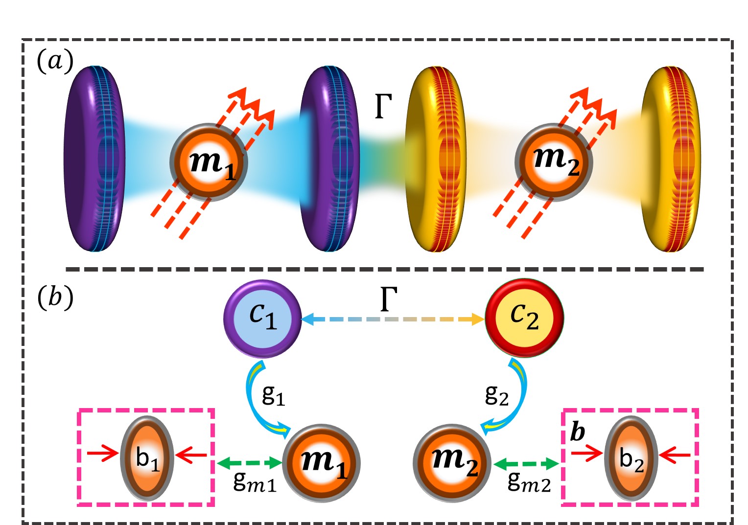
Figure 1: (Color Online) (a) Schematic diagram of the coupled cavity magnomechanical system in which each cavity mode contain a magnon mode in a YIG sphere couples that interact with the microwave cavity modes via magnetic dipole interaction and with phonon mode via magnetostrictive interaction. The magnetic field of the each microwave cavity modes is set to be along the x-direction, while the drive magnetic field (bias magnetic field) is considered along y-direction (z-direction). (b) The linear coupling diagram of each cavity magnomechanical system is shown. The two cavity modes are coupled via photon hoping $\Gamma$, while a cavity mode photon $c_{1}$ ($c_{2}$) is coupled to the magnon mode $m_{1}$ ($m_{2}$), with coupling strength $g_{1}$ ($g_{2}$), which then coupled to a phonon mode $b_{1}$ ($b_{2}$) to with magnomechanical coupling strength $g_{m1}$ ($g_{m2}$).

In the rotating wave approximation at the drive frequency $\omega_{0}$, he Hamiltonian of the system can be written as

$$H/\hbar = \sum_{k=1}^{2}\left[\Delta_{k}c_{k}c_{k}^{{\dagger}}+\Delta_{m_{k}}m_{k}^{{\dagger}}m_{k}+\frac{\omega_{b_{k}}}{2}\left(q_{k}^{2}+p_{k}^{2}\right)+g_{mk}m_{k}^{{\dagger}}m_{k}q_{k}+g_{k}\left(c_{k}m_{k}^{{\dagger}}+c_{k}^{{\dagger}}m_{k}\right)+i\Omega\left(m_{k}^{{\dagger}}-m_{k}\right)\right]$$

$$+\Gamma(c_{1}c_{2}^{{\dagger}}+c_{1}^{{\dagger}}c_{2}),$$

where $\Delta_{k}=\omega_{k}-\omega_{0k}$ ($k=1,2$) and $\Delta_{m_{k}}=\omega_{m}-\omega_{0k}$.

III Quantum dynamics and entanglement of the magnomechanical system

We now start to obtain the equations for the dynamics of this magnomechanical system. By incorporating the effect of noises and dissipations, the following set of quantum Langevin equations for the magnomechanical system can be obtained:

$$\dot{q}_{k} = \omega_{b_{k}}p_{k},$$ (7)

$$\dot{p}_{k} = -\omega_{b}q_{k}-\gamma_{b}p_{k}-g_{mk}m^{{\dagger}}_{k}m_{k}+\xi_{k},$$ (8)

$$\dot{c}_{k} = -\left(i\Delta_{k}+\kappa_{k}\right)c_{k}-ig_{k}m_{k}+\Gamma c_{j}+\sqrt{2\kappa_{a}}c_{k}^{in},(j\neq k)$$ (9)

$$\dot{m}_{k} = -\left(i\Delta_{m_{k}}+\kappa_{m}\right)m_{k}-ig_{k}c_{k}-ig_{mk}m_{k}q_{k}+\Omega_{k}+\sqrt{2\kappa_{m}}m^{in},$$ (10)

where $k_{k}$($k_{m}$) is the decay rate of the $k^{th}$ cavity mode (magnon mode) while $\gamma_{b}$ denotes the mechanical damping rate. $\xi$, $m^{in}$ and $c_{k}^{in}$ are input noise operators for the mechanical, magnon and cavity modes respectively. These noise operators are characterized by the following correlation functions [69]:

$$\left\langle\xi(t)\xi(t^{\prime})\right\rangle+\left\langle\xi(t^{\prime})\xi(t)\right\rangle/2 = \gamma_{b}[2n_{b}(\omega_{b})+1]\delta(t-t^{\prime}),$$ (11)

$$\left\langle c_{k}^{in}(t)c_{k}^{in{\dagger}}(t^{\prime})\right\rangle = [n_{k}(\omega_{k})+1]\delta(t-t^{\prime}),$$ (12)

$$\left\langle c_{k}^{in{\dagger}}(t)c_{k}^{in}(t^{\prime})\right\rangle = n_{k}(\omega_{k})\delta(t-t^{\prime}),$$ (13)

$$\left\langle m^{in{\dagger}}(t)m^{in}(t^{\prime})\right\rangle = n_{m}(\omega_{m})\delta(t-t^{\prime}),$$ (14)

$$\left\langle m^{in}(t)m^{in{\dagger}}(t^{\prime})\right\rangle = [n_{m}(\omega_{m})+1]\delta(t-t^{\prime}),$$ (15)

The equilibrium mean thermal photon, magnon, and phonon numbers are $n_{f}(\omega_{f})=[\exp(\frac{\hbar\omega_{f}}{k_{b}T})-1]^{-1}$ $[f=k(k=1,2),m,b]$, where $T$ is the environmental temperature and $k_{b}$ the Boltzmann constant.

If the magnon mode is strongly driven, then we must have $\left|\left\langle m\right\rangle\right|\gg 1$. In addition, the two MW cavity fields show large amplitudes due to the cavity-magnon beam splitter interactions. This permits us to linearize the above quantum Langevin equations by writing any operator as a sum of average value plus its fluctuation i.e., $o=\left\langle o\right\rangle+\delta o$, $(o=p,q,c_{k},m)$ and substitute it into Eq.(7-10). The average values of the dynamical operators are obtained as

$$\left\langle p_{k}\right\rangle = 0,$$ (16)

$$\left\langle q_{k}\right\rangle = \frac{-g_{mk}}{\omega_{b}}\left|\left\langle m_{k}\right\rangle\right|^{2},$$ (17)

$$\left\langle m_{j}\right\rangle = \frac{\Omega_{j}-ig_{k}\left\langle c_{k}\right\rangle}{i\Delta_{m_{k}}+\kappa_{m_{k}}},$$ (18)

$$\left\langle c_{1}\right\rangle = \frac{ig_{1}\Omega_{1}\alpha_{2}-\Gamma g_{2}\Omega_{2}(\kappa_{m_{1}}+i\Delta_{m_{1}})}{\alpha_{1}\alpha_{2}+\Gamma^{2}\left(i\Delta_{m_{1}}+\kappa_{m_{1}}\right)\left(i\Delta_{m_{2}}+\kappa_{m_{2}}\right)},$$ (19)

$$\left\langle c_{2}\right\rangle = \frac{ig_{2}\Omega_{2}\alpha_{1}-\Gamma g_{1}\Omega_{1}(\kappa_{m_{2}}+i\Delta_{m_{2}})}{\alpha_{1}\alpha_{2}+\Gamma^{2}\left(i\Delta_{m_{2}}+\kappa_{m_{2}}\right)\left(i\Delta_{m_{1}}+\kappa_{m_{1}}\right)},$$ (20)

where $\alpha_{j}=(i\Delta_{i}+\kappa_{i})(i\Delta_{m_{i}}+\kappa_{m_{i}})+g_{i}^{2}$ , $\Delta_{m}=\Delta_{m_{0}}+g_{mb}\left\langle q\right\rangle$ is the effective magnon mode detuning which includes the slight shift of frequency due to the magnomechanical interaction.

Now, we introduce the quadrature for the linearised quantum Langevin equations describing fluctuations are: $\delta x=\frac{1}{\sqrt{2}}(\delta m-\delta m^{{\dagger}})$, $\delta y=\frac{1}{\sqrt{2}i}(\delta m-\delta m^{{\dagger}})$, $\delta X_{k}=\frac{1}{\sqrt{2}}(\delta c_{k}-\delta c_{k}^{{\dagger}})$, $\delta Y_{k}=\frac{1}{\sqrt{2}i}(\delta c_{k}-\delta c_{k}^{{\dagger}})$ can be written in concise form as

$$\dot{\mathcal{F}}(t)=\mathcal{M}\mathcal{F}(t)+\mathcal{N}(t),$$ (21)

where $\mathcal{F}(t)$ and $\mathcal{N}(t)$ are, respectively, the quantum the fluctuation and input noise vectors and are given by:

$$\mathcal{F}(t) = [\delta C_{XY}(t),\delta M_{xy}(t),\delta Q_{qp}(t)]^{T},$$

$$\mathcal{N}(t) = [\mathcal{N}_{XY},\mathcal{N}_{xy},\mathcal{N}_{qp}]$$

where

$$\delta C_{XY}(t) = \delta X_{1}(t),\delta Y_{1}(t),\delta X_{2}(t),\delta Y_{2}(t)$$

$$\delta M_{xy}(t) = \delta x_{1}(t),\delta y_{1}(t),\delta x_{2}(t),\delta y_{2}(t)$$

$$\delta Q_{qp}(t) = \delta q_{1}(t),\delta p_{1}(t),\delta q_{2}(t),\delta p_{2}(t)$$

$$\mathcal{N}_{XY} = \sqrt{2k_{1}}X_{1}^{in}(t),\sqrt{2k_{1}}Y_{1}^{in}(t),\sqrt{2k_{2}}X_{2}^{in}(t),\sqrt{2k_{2}}Y_{2}^{in}(t)$$

$$\mathcal{N}_{xy} = \sqrt{2k_{m}}x_{1}^{in}(t),\sqrt{2k_{m}}y_{1}^{in}(t),\sqrt{2k_{m}}x_{2}^{in}(t),\sqrt{2k_{m}}y_{2}^{in}(t)$$

$$\mathcal{N}_{qp} = 0,\xi_{1}(t),0,\xi_{2}(t)$$

Furthermore, the drift matrix $\mathcal{M}$ can be written as

$$\mathcal{M}=\left[\begin{array}[]{cccccccccccc}-\kappa_{1}&\Delta_{1}&0&\Gamma&0&g_{1}&0&0&0&0&0&0\\ -\Delta_{1}&-\kappa_{1}&-\Gamma&0&-g_{1}&0&0&0&0&0&0&0\\ 0&\Gamma&-\kappa_{2}&\Delta_{2}&0&0&0&g_{2}&0&0&0&0\\ -\Gamma&0&-\Delta_{2}&-\kappa_{2}&0&0&-g_{2}&0&0&0&0&0\\ 0&g_{1}&0&0&-\kappa_{m_{1}}&\Delta_{m_{1}}&0&0&-G_{1}&0&0&0\\ -g_{1}&0&0&0&-\Delta_{m_{1}}&-\kappa_{m_{1}}&0&0&0&0&0&0\\ 0&0&0&g_{2}&0&0&-\kappa_{m_{2}}&\Delta_{m_{2}}&0&0&-G_{2}&0\\ 0&0&-g_{2}&0&0&0&-\Delta_{m_{2}}&-\kappa_{b_{2}}&0&0&0&0\\ 0&0&0&0&0&0&0&0&0&\omega_{b_{1}}&0&0\\ 0&0&0&0&0&G_{1}&0&0&-\omega_{b_{1}}&-\gamma_{b_{1}}&0&0\\ 0&0&0&0&0&0&0&0&0&0&0&\omega_{b_{2}}\\ 0&0&0&0&0&0&0&0&G_{2}&0&0&\gamma_{b_{2}}\end{array}\right],$$ (22)

where $G_{mb}=i\sqrt{2}g_{mb}\left\langle m\right\rangle$ is the effective magnomechanical coupling rate. By using Eq. (4), one can notice that effective magnomechanical coupling rate can be increased by applying strong magnon drive.

Next, we discuss the quantum correlation of bipartite subsystems with a special emphasis on the entanglement of two indirectly coupled modes and the two MW fields in the steady-state. The stability of the proposed system is the first prerequisite for the effectiveness of our scheme. According to Routh-Hurwitz criterion [70], the system is stable only if the real part of the all the eigenvalues of the drift matrix $\mathcal{M}$ are negative. Hence, we start our analysis by determining eigenvalues of the drift matrix $\mathcal{M}$ (i.e., $|\mathcal{M}-\lambda_{\mathcal{M}}\mathbb{1}|=0$) and make sure the stability condition are all satisfied in the following section (see Appendix A). The magnomechanical system presented here is characterized by $8\times 8$ covariance matrix V with its entries

$$V_{ij}(t)=\frac{1}{2}\left\langle F_{i}(t)F_{j}(t^{\prime})+F_{j}(t^{\prime})F_{i}(t)\right\rangle,$$ (23)

The covariance matrix of the magnomechanical system can be obtained from the steady state Lyapunov equation [71, 72]

$$\mathcal{M}V+V\mathcal{M}^{T}=-\mathcal{D},$$ (24)

where $\mathcal{D}=$ diag$[0,\gamma_{b}\left(2n_{b}+1\right),\kappa_{m}\left(2n_{m}+1\right),\kappa_{m}(2n_{m}+1)$ $\kappa_{1}\left(2n_{1}+1\right)$ ,$\kappa_{1}\left(2n_{1}+1\right)$, $\kappa_{2}\left(2n_{2}+1\right),\kappa_{2}\left(2n_{2}+1\right)]$, is a diagonal matrix which is called diffusion matrix and characterizes the noise correlations. The Lyapunov Eq. (24) as a linear equation for $V$ can be easily solved. Using the Simon condition for Gaussian states, we calculate the entanglement of the steady state [73, 74, 75, 76, 72].

$$E_{N}=\max[0,-\ln 2\eta^{-}],$$ (25)

where $\eta^{-}=$min eig$|\bigoplus^{2}_{j=1}(-\sigma_{y})\widetilde{\mathcal{V}_{4}}|$ is the minimum symplectic eigenvalue of covariance matrix and is $\widetilde{\mathcal{V}_{4}}=\varrho_{1|2}\mathcal{V}_{in}\varrho_{1|2}$, where $\mathcal{V}_{in}$ is a $4\times 4$ matrix of any two subsystems which can easily be obtain by neglecting the uninteresting rows and columns in $\mathcal{V}_{4}$. $\varrho_{1|2}=\sigma_{z}\bigoplus 1$=diag$(1,-1,1,1)$ is the matrix which characterizes the partial transposition at the level of covariance matrices. Here, $\sigma_{y}$ and $\sigma_{z}$ are the pauli spin matrices. Furthermore, a nonzero logarithmic negativity i.e., $E_{N}>0$ defines the presence of bipartite entanglement in our cavity magnomechanical system.

IV Results and Discussion

Parameters	Symbol	Value	Parameters	Symbol	Value
Phonon frequency	$\omega_{b}$	$2\pi\times$10 MHz	Cavity frequency	$\omega_{1}=\omega_{2}=\omega_{a}$	$2\pi\times$ 10 GHz
Cavity decay rates	$\kappa_{1}=\kappa_{2}=\kappa$	$2\pi\times$ 1 MHz	Magnon decay rate	$\kappa_{m}$	$2\pi\times$1 MHz
Mechanical damping rate	$\gamma_{b}$	$2\pi\times$100 Hz	Magnon-Microwave couplings	$\Gamma_{1}=\Gamma_{2}=\Gamma$	$2\pi\times$3.2 MHz
Magnomechanical coupling	$g_{mb}$	$2\pi\times$0.3 Hz	Drive Magnetic Field	B	$3.9\times 10^{-5}$T
YIG Sphere Diameter	D	250 $\mu$m	Temperature	T	10 mK
Power	$\wp=\frac{B^{2}\pi r^{2}c}{2\mu^{2}}$	9.8 mW	Spin density	$\rho$	$4.22\times 10^{27}m^{-3}$

Table 1: Parameters used in recent experiments for the mechanical resonators

Bipartite Subsystem	Entanglement Symbol	Bipartite Subsystem	Entanglement Symbol
Cavity 1-Cavity 2	$E_{c-c}^{N}$
Cavity 1-magnon 2	$E^{N}_{c_{1}-m_{2}}$	Cavity 2-magnon 1	$E^{N}_{c_{2}-m_{1}}$
Cavity 1-phonon 2	$E^{N}_{c_{1}-b_{2}}$	Cavity 2-phonon 1	$E^{N}_{c_{2}-b_{1}}$

Table 2: Adopted notation for the different bipartite subsystem entanglement.

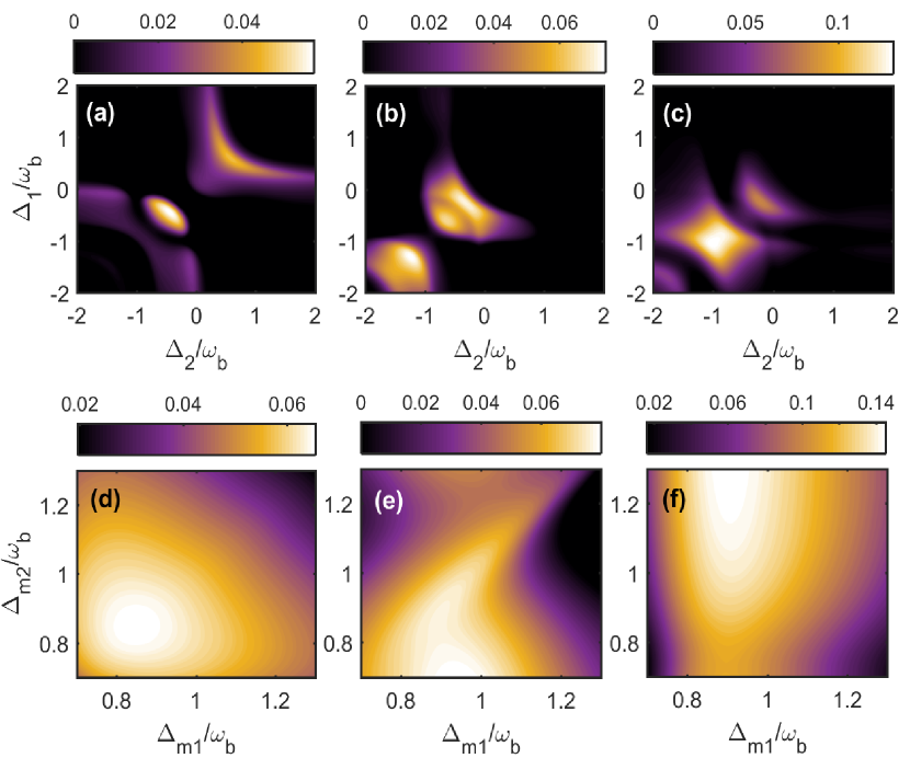
Figure 2: (Color Online) Density plot of bipartite entanglement in (a),(d) $E_{c_{1}-c_{2}}^{N}$; in (b),(e) $E_{c_{1}-m_{2}}^{N}=E_{c_{2}-m_{1}}^{N}$ and in (c),(f) $E_{c_{1}-b_{2}}^{N}=E_{c_{2}-b_{1}}^{N}$ versus cavity detunings $\Delta_{1}/\omega_{b}$ and $\Delta_{2}/\omega_{b}$ in (a)-(c) for $\Delta_{m_{1}}=\Delta_{m_{2}}=\omega_{b}$ whereas varying both magnon detunings $\Delta_{m_{1}}/\omega_{b}$ and $\Delta_{m_{2}}/\omega_{b}$ in (d)-(f). We use optimum values of of $\Delta_{1}$ and $\Delta_{2}$ for (d)-(f). The other parameters are given in Table 1.

In this section we are going to discuss in details the results of bipartite entanglements as we have six different modes in this coupled cavity Magnomechnical system. So, we can get bipartite entanglement in any of two modes however the most significant part of our study is to investigate the bipartite entanglement present in various spatially distant subsystems which we have summarised in Table 2 with symbols.
In Fig. 2, we present five different distant bipartite entanglements as a function of dimensionless cavity detuning for first cavity $\Delta_{1}/\omega_{b}$ and second cavity $\Delta_{2}/\omega_{b}$. When both the magnon detuning is kept in resonant with blue sideband regime i.e. $\Delta_{m_{1}}=\Delta_{m_{2}}=\omega_{b}$ it can be seen that bipartite entanglement between two cavity modes $E_{c_{1}-c_{2}}^{N}$ become maximum for $\Delta_{1}=\Delta_{2}=-0.5\omega_{b}$ although even if both the cavities are resonant with blue sideband regime i.e. $\Delta_{1}=\Delta_{2}=\omega_{b}$ we have significant amount of bipartite entanglement in $E_{c_{1}-c_{2}}^{N}$ as shown in Fig. 2(a). In Fig.2(b) we study the bipartite entanglement $E_{c_{1}-m_{2}}^{N}\textbf{(}E_{c_{2}-m_{1}}^{N}\text{)}$ which attains maximum value either when both the cavities are resonant with driving field, i.e. $\Delta_{1}=\Delta_{2}=0$ or resonant with red sideband regime, i.e. $\Delta_{1}=\Delta_{2}=-\omega_{b}$. Moreover when both the cavities are kept in resonant with this red sideband regime the bipartite entanglement $E_{c_{1}-b_{2}}^{N}\textbf{(}E_{c_{2}-b_{1}}^{N}\textbf{)}$ attains its maximum value as shown in Fig. 2(c). Furthermore, it can be seen that if cavity detunigs for both the cavities are kept fixed and resonant with blue sideband regime i.e. $\Delta_{1}=\Delta_{2}=\omega_{b}$ then all the above mentioned bipartite entanglements have significant values on gradually varying both $\Delta_{m_{1}}/\omega_{b}$ and $\Delta_{m_{2}}/\omega_{b}$ from 0.8 to 1.1 as shown in Fig. 2(d)-2(f).

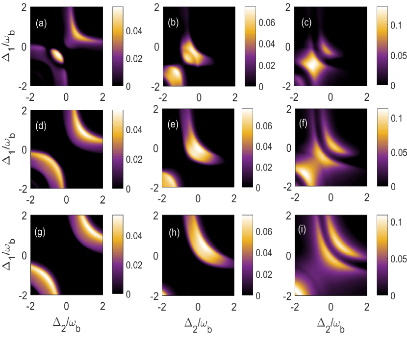
Figure 3: (Color Online) Density plot of bipartite entanglement in (a),(d),(g) $E_{c_{1}-c_{2}}^{N}$; in (b),(e),(h) $E_{c_{1}-m_{2}}^{N}=E_{c_{2}-m_{1}}^{N}$ and in (c),(f),(i) $E_{c_{1}-b_{2}}^{N}=E_{c_{2}-b_{1}}^{N}$ versus detunings $\Delta_{1}/\omega_{b}$ and $\Delta_{2}/\omega_{b}$. Here we have taken $\Gamma=0.5\omega_{b}$ for (a),(b),(c); $\Gamma=0.8\omega_{b}$ for (d),(e),(f) and $\Gamma=\omega_{b}$ for (g),(h),(i). We take both magnon detunings at $\Delta_{m_{1}}=\Delta_{m_{2}}=\omega_{b}$ The other parameters are given in Table 1

We plot five different distant bipartite entanglements as a function of $\Delta_{1}/\omega_{b}$ and $\Delta_{2}/\omega_{b}$ for different photon hopping factor $\Gamma$ as well while keepin both the magnon detuning in resonant with blue sideband regime i.e. $\Delta_{m_{1}}=\Delta_{m_{2}}=\omega_{b}$ in Fig. 3. For $\Gamma==0.5\omega_{b}$ the quantity $E_{c_{1}-c_{2}}^{N}$ attains maximum value when both the cavity have zero detunings i.e. $\Delta_{1}=\Delta_{2}=0$ whereas for off resonant cavities we get finite values of $E_{c_{1}-c_{2}}^{N}$ as shown in Fig. 3(a). However the quantities $E_{c_{1}-m_{2}}^{N}=E_{c_{2}-m_{1}}^{N}$ become maximum for two values of cavity detunings which are $\Delta_{1}=\Delta_{2}=0$ and $\Delta_{1}=\Delta_{2}=-\omega_{b}$ as shown in Fig. 3(b) whereas both the quantities $E_{c_{1}-b_{2}}^{N}=E_{c_{2}-b_{1}}^{N}$ become maximum at $\Delta_{1}=\Delta_{2}=-\omega_{b}$ as shown in Fig. 3(c). It can be seen that if we increase photon hopping factor upto $\Gamma==0.8\omega_{b}$ then the bipartite entanglement in between both the cavity modes $E_{c_{1}-c_{2}}^{N}$ becomes maximum for two cases i.e. for resonant cavities $\Delta_{1}=\Delta_{2}=0$ and when resonant with red sideband regime $\Delta_{1}=\Delta_{2}=-\omega_{b}$ as shown in Fig. 3(d). In addition, in the density plots of the quantities $E_{c_{1}-m_{2}}^{N}=E_{c_{2}-m_{1}}^{N}$ the panel corresponding to red sideband regime start to decrease whereas the panel corresponding to resonant cavities increases as shown in Fig. 3(e). Moreover, the quantities $E_{c_{1}-b_{2}}^{N}=E_{c_{2}-b_{1}}^{N}$ show the finite values for a broad range of cavity detunings and attain maximum value for $\Delta_{1}=\Delta_{2}=-1.5\omega_{b}$ as shown in Fig. 3(f). On further increasing the value of $\Gamma$ and keeping it at $\Gamma==\omega_{b}$, the quantity $E_{c_{1}-c_{2}}^{N}$ again becomes maximum for two cases i.e. for $\Delta_{1}=\Delta_{2}=-0.5\omega_{b}$ and $\Delta_{1}=\Delta_{2}=-1.5\omega_{b}$ as shown in Fig. 3(g) whereas the quantities $E_{c_{1}-m_{2}}^{N}=E_{c_{2}-m_{1}}^{N}$ attain maximum value only when both the cavity detunings are nearly resonant with blue sideband regime as given in Fig. 3(h). However the quantities $E_{c_{1}-b_{2}}^{N}=E_{c_{2}-b_{1}}^{N}$ attain maximum value only for very far off-resonant cavities $\Delta_{1}=\Delta_{2}=-2\omega_{b}$ whereas for a broad range of negative cavity detunings both these distant entanglements almost become negligible however for a positive value of $\Delta_{1}/\omega_{b}$ and $\Delta_{2}/\omega_{b}$ both the bipartite entanglements attain finite values $E_{c_{1}-b_{2}}^{N}=E_{c_{2}-b_{1}}^{N}$ as shown in Fig. 3(i).

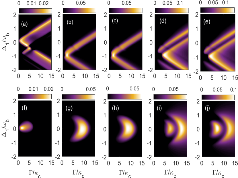
Figure 4: (Color Online) Density plot of bipartite entanglement in (a),(f) $E^{N}_{c_{1}-c_{2}}$; in (b),(g) $E^{N}_{c_{1}-m_{2}}$; in (c),(h) $E^{N}_{c_{2}-m_{1}}$; in (d),(i) $E^{N}_{c_{1}-b_{2}}$ and (e),(j) $E^{N}_{c_{2}-b_{1}}$ versus $\Delta_{1}/\omega_{b}$ and $\Gamma/\omega_{b}$ for $\Delta_{2}=\omega_{b}$ in (a)-(e) and for $\Delta_{2}=-\omega_{b}$ in (f)-(j). The other parameters are same as in Fig. 3.

We study the effects of varying photon hopping factor $\Gamma/\kappa_{c}$ and normalised cavity detuning $\Delta_{1}/\omega_{b}$ on these five bipartite entanglements while keeping second cavity detuning $\Delta_{2}/\omega_{b}$ fixed in Fig. 4. It can be seen that for $\Delta_{2}=\omega_{b}$ i.e. when second cavity detuning is resonant with blue sideband regime, the quantity $E_{c_{1}-c_{2}}^{N}$ becomes maximum for $\Delta_{1}$ varying in the range of $0--0.5\omega_{b}$ whereas photon hopping factor varies upto $0-5$ although after this range $E_{c_{1}-b_{2}}^{N}=E_{c_{2}-b_{1}}^{N}$ get finite value for both positive and negative $\Delta_{1}/\omega_{b}$ with varying $\Gamma\kappa_{c}$ as shown in Fig. 4(a). Similarly both the quantities $E^{N}_{c_{1}-m_{2}}$ and $E^{N}_{c_{2}-m_{1}}$ get maximum for $\Delta_{1}\approx-\omega_{b}$ and after this they attain finite values again on varying $\Delta_{1}/\omega_{b}$ and $\Gamma\kappa_{c}$ as shown in Fig. 4(b) and 4(c). Moreover, the other two quantities $E_{c_{1}-b_{2}}^{N}$ and $E_{c_{2}-b_{1}}^{N}$ attain their maximum value for $\Delta_{1}/\omega_{b}$ varying in the range of $(-1)$ to $(-2)$ even for a very high value of $\Gamma\kappa_{c}$ as shown in Fig. 4 (d) and 4(e). In another scenario for $\Delta_{2}=-\omega_{b}$ i.e. when second cavity detuning is resonant with red sideband regime, the quantity $E_{c_{1}-c_{2}}^{N}$ becomes maximum nearby to $\Delta_{1}/\omega_{b}=0$ and $\Gamma\approx\kappa_{c}$ however after this it decreases very rapidly on gradually increasing $\Delta_{1}/\omega_{b}$ as well as $\Gamma/\kappa_{c}$ as shown in Fig. 4(f). For this value of second cavity detuning, it can be seen that both the bipartite entanglements $E^{N}_{c_{1}-m_{2}}$ as well as $E^{N}_{c_{2}-m_{1}}$ get maximum only around $\Delta_{1}/\omega_{b}=0$ to $\pm 1.0$ and $\Gamma/\kappa_{c}$ value lies in between 7-10 and afterwards both these entanglements vanish as shown in Figs. 4(g) and 4(h). However in this range of $\Delta_{1}/\omega_{b}$, $E_{c_{1}-b_{2}}^{N}$ and $E_{c_{2}-b_{1}}^{N}$ first become maximum for single photon hopping factor $\Gamma/\kappa_{c}$ values which are in between the range 5-7 and then both the bipartite entanglements become zero although a further increase in $\Gamma/\kappa_{c}$ give maximum values of $E_{c_{1}-b_{2}}^{N}$ and $E_{c_{2}-b_{1}}^{N}$ as depicted in Figs. 4(i) and 4(j).

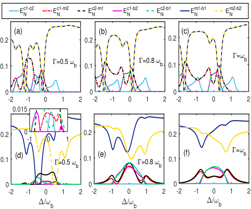
Figure 5: (Color Online) Plot of different bipartite entanglement versus $\Delta/\omega_{b}$ by taking $\Delta=\Delta_{1}=\Delta_{2}=\omega_{b}$ for the upper panel and $\Delta=\Delta_{1}=-\Delta_{2}=\omega_{b}$ for the lower panel. The other parameters are as in Fig. 3.

Furthermore, in Fig. 5 we plot different distant bipartite entanglements as a function of $\Delta/\omega_{b}$ for symmetric cavities where we take $\Delta=\Delta_{1}=\Delta_{2}=\omega_{b}$ (upper panel) and for antisymmetric cavities $\Delta=\Delta_{1}=-\Delta_{2}=\omega_{b}$ (lower panel). For $\Gamma=0.5\omega_{b}$ and symmetric cavities, the bipartite quantity $E_{c_{1}-c_{2}}^{N}$ varies from 0 to 0.6 with gradually changing the normalised detuning $\Delta/\omega_{b}$ in between -1 to 1 and after this range the quantity $E_{c_{1}-c_{2}}^{N}$ becomes zero as shown in Fig. 5(a). However, the other bipartite quantities $E_{m_{2}-b_{2}}^{N}$ $(E_{m_{1}-b_{1}}^{N})$ varies from 0 to 0.2 for negative values of $\Delta/\omega_{b}$ and for $\Delta/\omega_{b}$ greater than zero both of these quantities get saturated to a finite positive value. Moreover, the other bipartite quantities $E_{c_{1}-b_{2}}^{N}$ ($E_{c_{2}-b_{1}}^{N}$) as well as $E_{c_{1}-m_{2}}^{N}$ ($E_{c_{2}-m_{1}}^{N}$) become almost zero for positive values of $\Delta/\omega_{b}$ as shown in Fig. 5(a). It can be seen that for this value of $\Gamma$ a significant amount of entanglement transfer takes place from $E_{m_{2}-b_{2}}^{N}$ $(E_{m_{1}-b_{1}}^{N})$ to $E_{c_{1}-b_{2}}^{N}$ ($E_{c_{2}-b_{1}}^{N}$) and $E_{c_{1}-m_{2}}^{N}$ ($E_{c_{2}-m_{1}}^{N}$) at $\Delta/\omega_{b}$ $\approx$ -0.3 and -1.2. For $\Gamma=0.8\omega_{b}$, the bipartite entanglement $E_{c_{1}-c_{2}}^{N}$ become finite for $\Delta/\omega_{b}$ varying in the range of (0.3)-(1.3) and (-0.5)-(-1.3) as shown in Fig. 5(b). It can be also seen that the bipartite quantities $E_{m_{2}-b_{2}}^{N}$ $(E_{m_{1}-b_{1}}^{N})$ almost get around 0.2 for positive as well as negative values of $\Delta/\omega_{b}$ except for certain values of $\Delta/\omega_{b}\approx 0.2$ and $-1.5$ whereas $E_{c_{1}-m_{2}}^{N}$ ($E_{c_{2}-m_{1}}^{N}$) has finite values upto $\Delta/\omega_{b}\approx 0.5$ and $E_{c_{1}-b_{2}}^{N}$ ($E_{c_{2}-b_{1}}^{N}$) becomes zero even for negative values of $\Delta/\omega_{b}$. In this case we get maximum entanglement transfer from $E_{m_{2}-b_{2}}^{N}$ $(E_{m_{1}-b_{1}}^{N})$ to $E_{c_{1}-b_{2}}^{N}$ ($E_{c_{2}-b_{1}}^{N}$) and $E_{c_{1}-m_{2}}^{N}$ ($E_{c_{2}-m_{1}}^{N}$) around $\Delta/\omega_{b}$ $\approx$ 0.1 and -1.5. If we increase further single photon hopping factor upto $\Gamma=\omega_{b}$ then the quantity $E_{c_{1}-c_{2}}^{N}$ remains finite only for $\Delta/\omega_{b}$ varying in the range of $(0.5)-(1.5)$ as well as $(-0.5)-(-1.5)$ whereas $E_{m_{2}-b_{2}}^{N}$ $(E_{m_{1}-b_{1}}^{N})$ almost gets around 0.25 except at certain values of the $\Delta/\omega_{b}$ for which the entanglement transfer takes place between different bipartite correlations as shown in Fig. 5(c). In this case $E_{c_{1}-m_{2}}^{N}$ ($E_{c_{2}-m_{1}}^{N}$) has finite values upto $\Delta/\omega_{b}\approx 1.0$ however $E_{c_{1}-b_{2}}^{N}$ ($E_{c_{2}-b_{1}}^{N}$) qualitatively remains the same as depicted in Fig. 5(c). Moreover, the maximum entanglement transfer from $E_{m_{2}-b_{2}}^{N}$ $(E_{m_{1}-b_{1}}^{N})$ to $E_{c_{1}-b_{2}}^{N}$ ($E_{c_{2}-b_{1}}^{N}$) and $E_{c_{1}-m_{2}}^{N}$ ($E_{c_{2}-m_{1}}^{N}$) takes place around values $\Delta/\omega_{b}$ $\approx$ 0.5 and -1.8. Now for antisymmetric cavities $\Delta=\Delta_{1}=-\Delta_{2}=\omega_{b}$ and $\Gamma=0.5\omega_{b}$ it can be seen that both the bipartite entanglements $E_{m_{2}-b_{2}}^{N}$ $(E_{m_{1}-b_{1}}^{N})$ have finite values with a varying $\Delta/\omega_{b}$ although for few values both becomes zero s shown in Fig. 5(d). All other bipartite entanglements have very small values for this value of $\Gamma$. For $\Gamma=0.8\omega_{b}$ the bipartite entanglement $E_{c_{1}-c_{2}}^{N}$ becomes zero whereas the quantities $E_{m_{2}-b_{2}}^{N}$ $(E_{m_{1}-b_{1}}^{N})$ have finite values from 0.1-0.25 as shown in Fig. 5(d). Moreover, the bipartite entanglements $E_{c_{1}-b_{2}}^{N}$ ($E_{c_{2}-b_{1}}^{N}$) increases for this value of $\Gamma$ and become finite for a varying $\Delta/\omega_{b}$ in between the range of (-1)-(1) whereas $E_{c_{1}-m_{2}}^{N}$ ($E_{c_{2}-m_{1}}^{N}$) also increases and varies from 0-0.07(0.08) with $\Delta/\omega_{b}$ as depicted in Fig. 5(d). With a further increment in $\Gamma$ both the bipartite entanglements $E_{c_{1}-m_{2}}^{N}$ ($E_{c_{2}-m_{1}}^{N}$) becomes finite over whole range of varying $\Delta/\omega_{b}$ whereas all other bipartite entanglements qualitatively remains the same (like earlier case of $\Gamma=0.8\omega_{b}$) as shown in Fig. 5(f).

V Conclusions

We present an experimentally feasible scheme based on coupled magnomechanical system where two microwave cavities are coupled through single photon hopping parameter $\Gamma$ and each cavity also contains a magnon mode and phonon mode. We have investigated continuous variable entanglement between distant bipartitions for an appropriate set of both cavities and magnons detuning and their decay rates. Hence, it can be seen that bipartite entanglement between indirectly coupled systems are substantial in our proposed scheme. Moreover, cavity-cavity coupling strength also plays a key role in the degree of bipartite entanglement and its transfer among different direct and indirect modes. This scheme may prove to be significant for processing continuous variable quantum information in quantum memory protocols.

Appendix A. Stability of the system

It is worthy to discuss the stability of the subject system, since the stability of strongly magnomechanical system is difficult to achieve. In this section, we are going to discuss the stability of our system. The system becomes stable only when all the eigenvalues of the drift matrix $\mathcal{M}$ have negative real parts. In case the sign of the real part of eigenvalues changes, system will becomes unstable. Hence, in order to provide the intuitive picture for the parameter regime where stability occurs can be obtained from the Routh-Hurwitz criterion, we have plotted the maximum of the real parts of the eigenvalues $\lambda_{\mathcal{M}}$ ($|\mathcal{M}-\lambda_{\mathcal{M}}\mathbb{1}|=0$) of the drift matrix $\mathcal{M}$ vs the normalized detunings in Fig. 7 [70]. It is important to mention here that the system becomes unstable if the maximum of the real parts of the eigenvalues $\lambda_{\mathcal{M}}$ is greater than zero. Figure. 7 clearly shows the maximum of the real parts of the eigenvalues $\lambda_{\mathcal{M}}$ remains negative for the chosen parameters and hence the system is stable. Therefore, the whole set of numerical parameters used throughout the manuscript satisfies the stability conditions and hence the working regime we chose is the regime of stability.

Data availability

All data used during this study are available within the article.

References

References

- Schwabl [2007] F. Schwabl, Quantum mechanics (Springer Science & Business Media, 2007).
- Ballentine [2014] L. E. Ballentine, Quantum mechanics: a modern development (World Scientific Publishing Company, 2014).
- Horodecki et al. [2009] R. Horodecki, P. Horodecki, M. Horodecki, and K. Horodecki, Quantum entanglement, Reviews of modern physics 81, 865 (2009).
- Vitali et al. [2007] D. Vitali, S. Gigan, A. Ferreira, H. Böhm, P. Tombesi, A. Guerreiro, V. Vedral, A. Zeilinger, and M. Aspelmeyer, Optomechanical entanglement between a movable mirror and a cavity field, Physical review letters 98, 030405 (2007).
- Mancini et al. [2002] S. Mancini, V. Giovannetti, D. Vitali, and P. Tombesi, Entangling macroscopic oscillators exploiting radiation pressure, Physical review letters 88, 120401 (2002).
- Yang et al. [2015] C.-J. Yang, J.-H. An, W. Yang, and Y. Li, Generation of stable entanglement between two cavity mirrors by squeezed-reservoir engineering, Physical Review A 92, 062311 (2015).
- Li et al. [2017] J. Li, G. Li, S. Zippilli, D. Vitali, and T. Zhang, Enhanced entanglement of two different mechanical resonators via coherent feedback, Physical Review A 95, 043819 (2017).
- Hartmann and Plenio [2008] M. J. Hartmann and M. B. Plenio, Steady state entanglement in the mechanical vibrations of two dielectric membranes, Physical Review Letters 101, 200503 (2008).
- Liao et al. [2014] J.-Q. Liao, Q.-Q. Wu, F. Nori, et al., Entangling two macroscopic mechanical mirrors in a two-cavity optomechanical system, Physical Review A 89, 014302 (2014).
- Xiong et al. [2005] H. Xiong, M. O. Scully, and M. S. Zubairy, Correlated spontaneous emission laser as an entanglement amplifier, Physical review letters 94, 023601 (2005).
- Kiffner et al. [2007] M. Kiffner, M. S. Zubairy, J. Evers, and C. Keitel, Two-mode single-atom laser as a source of entangled light, Physical Review A 75, 033816 (2007).
- Qamar et al. [2009] S. Qamar, M. Al-Amri, S. Qamar, and M. S. Zubairy, Entangled radiation via a raman-driven quantum-beat laser, Physical Review A 80, 033818 (2009).
- Chen et al. [2019] Z. Chen, J.-X. Peng, J.-J. Fu, and X.-L. Feng, Entanglement of two rotating mirrors coupled to a single laguerre-gaussian cavity mode, Optics express 27, 29479 (2019).
- Bhattacharya et al. [2008] M. Bhattacharya, P.-L. Giscard, and P. Meystre, Entanglement of a laguerre-gaussian cavity mode with a rotating mirror, Physical Review A 77, 013827 (2008).
- Peng et al. [2019] J.-X. Peng, Z. Chen, Q.-Z. Yuan, and X.-L. Feng, Optomechanically induced transparency in a laguerre-gaussian rotational-cavity system and its application to the detection of orbital angular momentum of light fields, Physical Review A 99, 043817 (2019).
- Singh et al. [2021] S. Singh, J.-X. Peng, M. Asjad, and M. Mazaheri, Entanglement and coherence in a hybrid laguerre–gaussian rotating cavity optomechanical system with two-level atoms, Journal of Physics B: Atomic, Molecular and Optical Physics 54, 215502 (2021).
- Cheng et al. [2021] H.-J. Cheng, S.-J. Zhou, J.-X. Peng, A. Kundu, H.-X. Li, L. Jin, and X.-L. Feng, Tripartite entanglement in a laguerre–gaussian rotational-cavity system with an yttrium iron garnet sphere, JOSA B 38, 285 (2021).
- Rameshti et al. [2022] B. Z. Rameshti, S. V. Kusminskiy, J. A. Haigh, K. Usami, D. Lachance-Quirion, Y. Nakamura, C.-M. Hu, H. X. Tang, G. E. Bauer, and Y. M. Blanter, Cavity magnonics, Physics Reports 979, 1 (2022).
- Rao et al. [2021] J. Rao, P. Xu, Y. Gui, Y. Wang, Y. Yang, B. Yao, J. Dietrich, G. Bridges, X. Fan, D. Xue, et al., Interferometric control of magnon-induced nearly perfect absorption in cavity magnonics, Nature communications 12, 1933 (2021).
- Zhang et al. [2021] G.-Q. Zhang, Z. Chen, W. Xiong, C.-H. Lam, and J. You, Parity-symmetry-breaking quantum phase transition via parametric drive in a cavity magnonic system, Physical Review B 104, 064423 (2021).
- Shen et al. [2021] R.-C. Shen, Y.-P. Wang, J. Li, S.-Y. Zhu, G. Agarwal, and J. You, Long-time memory and ternary logic gate using a multistable cavity magnonic system, Physical Review Letters 127, 183202 (2021).
- Tabuchi et al. [2014a] Y. Tabuchi, S. Ishino, T. Ishikawa, R. Yamazaki, K. Usami, and Y. Nakamura, Hybridizing ferromagnetic magnons and microwave photons in the quantum limit, Physical review letters 113, 083603 (2014a).
- Zhang et al. [2014a] X. Zhang, C.-L. Zou, L. Jiang, and H. X. Tang, Strongly coupled magnons and cavity microwave photons, Physical review letters 113, 156401 (2014a).
- Kittel [1948a] C. Kittel, On the theory of ferromagnetic resonance absorption, Physical review 73, 155 (1948a).
- Li et al. [2023] J. Li, Y.-P. Wang, J.-Q. You, and S.-Y. Zhu, Squeezing microwaves by magnetostriction, National Science Review 10, nwac247 (2023).
- Li et al. [2018] J. Li, S.-Y. Zhu, and G. Agarwal, Magnon-photon-phonon entanglement in cavity magnomechanics, Physical review letters 121, 203601 (2018).
- Ullah et al. [2020] K. Ullah, M. T. Naseem, and Ö. E. Müstecaplıoğlu, Tunable multiwindow magnomechanically induced transparency, fano resonances, and slow-to-fast light conversion, Physical Review A 102, 033721 (2020).
- Sohail et al. [2023a] A. Sohail, R. Ahmed, J.-X. Peng, T. Munir, A. Shahzad, S. Singh, and M. C. de Oliveira, Controllable fano-type optical response and four-wave mixing via magnetoelastic coupling in an opto-magnomechanical system, Journal of Applied Physics 133 (2023a).
- Liu et al. [2023] Z.-X. Liu, J. Peng, and H. Xiong, Generation of magnonic frequency combs via a two-tone microwave drive, Physical Review A 107, 053708 (2023).
- Singh et al. [2023] S. Singh, M. Mazaheri, J.-X. Peng, A. Sohail, M. Khalid, and M. Asjad, Enhanced weak force sensing based on atom-based coherent quantum noise cancellation in a hybrid cavity optomechanical system, Frontiers in Physics 11, 245 (2023).
- Amazioug et al. [2023] M. Amazioug, B. Teklu, and M. Asjad, Enhancement of magnon–photon–phonon entanglement in a cavity magnomechanics with coherent feedback loop, Scientific Reports 13, 3833 (2023).
- Zhang et al. [2015] X. Zhang, C.-L. Zou, N. Zhu, F. Marquardt, L. Jiang, and H. X. Tang, Magnon dark modes and gradient memory, Nature communications 6, 8914 (2015).
- Shen et al. [2022] R.-C. Shen, J. Li, Z.-Y. Fan, Y.-P. Wang, and J. You, Mechanical bistability in kerr-modified cavity magnomechanics, Physical Review Letters 129, 123601 (2022).
- Wang et al. [2018] Y.-P. Wang, G.-Q. Zhang, D. Zhang, T.-F. Li, C.-M. Hu, and J. You, Bistability of cavity magnon polaritons, Physical review letters 120, 057202 (2018).
- Kong et al. [2019] C. Kong, H. Xiong, and Y. Wu, Magnon-induced nonreciprocity based on the magnon kerr effect, Physical Review Applied 12, 034001 (2019).
- Zhang et al. [2023] G.-Q. Zhang, Y. Wang, and W. Xiong, Detection sensitivity enhancement of magnon kerr nonlinearity in cavity magnonics induced by coherent perfect absorption, Physical Review B 107, 064417 (2023).
- Xiong et al. [2022] W. Xiong, M. Tian, G.-Q. Zhang, and J. You, Strong long-range spin-spin coupling via a kerr magnon interface, Physical Review B 105, 245310 (2022).
- Wang et al. [2016] Y.-P. Wang, G.-Q. Zhang, D. Zhang, X.-Q. Luo, W. Xiong, S.-P. Wang, T.-F. Li, C.-M. Hu, and J. You, Magnon kerr effect in a strongly coupled cavity-magnon system, Physical Review B 94, 224410 (2016).
- Zhang et al. [2019a] G. Zhang, Y. Wang, and J. You, Theory of the magnon kerr effect in cavity magnonics, Science China Physics, Mechanics & Astronomy 62, 1 (2019a).
- Hisatomi et al. [2016] R. Hisatomi, A. Osada, Y. Tabuchi, T. Ishikawa, A. Noguchi, R. Yamazaki, K. Usami, and Y. Nakamura, Bidirectional conversion between microwave and light via ferromagnetic magnons, Physical Review B 93, 174427 (2016).
- Yan et al. [2020] Z. Yan, C. Wan, and X. Han, Magnon blocking effect in an antiferromagnet-spaced magnon junction, Physical Review Applied 14, 044053 (2020).
- Liu et al. [2019] Z.-X. Liu, H. Xiong, and Y. Wu, Magnon blockade in a hybrid ferromagnet-superconductor quantum system, Physical Review B 100, 134421 (2019).
- Yu et al. [2020] M. Yu, H. Shen, and J. Li, Magnetostrictively induced stationary entanglement between two microwave fields, Physical Review Letters 124, 213604 (2020).
- Hidki et al. [2023a] A. Hidki, A. Lakhfif, J. El Qars, and M. Nassik, Evolution of rényi-2 quantum correlations in a double cavity–magnon system, Modern Physics Letters A , 2350044 (2023a).
- Li and Zhu [2019] J. Li and S.-Y. Zhu, Entangling two magnon modes via magnetostrictive interaction, New Journal of Physics 21, 085001 (2019).
- Zhang et al. [2019b] Z. Zhang, M. O. Scully, and G. S. Agarwal, Quantum entanglement between two magnon modes via kerr nonlinearity driven far from equilibrium, Physical Review Research 1, 023021 (2019b).
- Yang et al. [2020] Z.-B. Yang, J.-S. Liu, H. Jin, Q.-H. Zhu, A.-D. Zhu, H.-Y. Liu, Y. Ming, and R.-C. Yang, Entanglement enhanced by kerr nonlinearity in a cavity optomagnonics system, Optics Express 28, 31862 (2020).
- Hussain et al. [2022] B. Hussain, S. Qamar, and M. Irfan, Entanglement enhancement in cavity magnomechanics by an optical parametric amplifier, Physical Review A 105, 063704 (2022).
- Hidki et al. [2023b] A. Hidki, Y.-L. Ren, A. Lakhfif, J. El Qars, and M. Nassik, Enhanced maximum entanglement between two microwave fields in the cavity magnomechanics with an optical parametric amplifier, Physics Letters A 463, 128667 (2023b).
- Sohail et al. [2023b] A. Sohail, R. Ahmed, J.-X. Peng, A. Shahzad, and S. Singh, Enhanced entanglement via magnon squeezing in a two-cavity magnomechanical system, JOSA B 40, 1359 (2023b).
- Hidki et al. [2023c] A. Hidki, A. Lakhfif, J. El Qars, and M. Nassik, Transfer of squeezing in a cavity magnomechanics system, Journal of Modern Optics , 1 (2023c).
- Wu et al. [2021] W.-J. Wu, Y.-P. Wang, J.-Z. Wu, J. Li, and J. You, Remote magnon entanglement between two massive ferrimagnetic spheres via cavity optomagnonics, Physical Review A 104, 023711 (2021).
- Sun et al. [2021] F.-X. Sun, S.-S. Zheng, Y. Xiao, Q. Gong, Q. He, and K. Xia, Remote generation of magnon schrödinger cat state via magnon-photon entanglement, Physical Review Letters 127, 087203 (2021).
- Xie et al. [2023] H. Xie, L.-W. He, C.-G. Liao, Z.-H. Chen, and X.-M. Lin, Generation of robust optical entanglement in cavity optomagnonics, Optics Express 31, 7994 (2023).
- Chen et al. [2021] Y.-T. Chen, L. Du, Y. Zhang, and J.-H. Wu, Perfect transfer of enhanced entanglement and asymmetric steering in a cavity-magnomechanical system, Physical Review A 103, 053712 (2021).
- Dilawaiz and Irfan [2022] S. Q. Dilawaiz and M. Irfan, Entangled atomic ensemble and yig sphere in coupled microwave cavities, arXiv preprint arXiv:2211.14914 (2022).
- Zhang et al. [2016] X. Zhang, C. Zou, L. Jiang, and H. Tang, Cavity magnomechanics sci, Adv 2, e1501286 (2016).
- Li et al. [2019] J. Li, S.-Y. Zhu, and G. Agarwal, Squeezed states of magnons and phonons in cavity magnomechanics, Physical Review A 99, 021801 (2019).
- Kittel [1958] C. Kittel, Interaction of spin waves and ultrasonic waves in ferromagnetic crystals, Physical Review 110, 836 (1958).
- Zhang et al. [2014b] X. Zhang, C.-L. Zou, L. Jiang, and H. X. Tang, Strongly coupled magnons and cavity microwave photons, Physical review letters 113, 156401 (2014b).
- Gonzalez-Ballestero et al. [2020] C. Gonzalez-Ballestero, D. Hümmer, J. Gieseler, and O. Romero-Isart, Theory of quantum acoustomagnonics and acoustomechanics with a micromagnet, Physical Review B 101, 125404 (2020).
- Osada et al. [2016] A. Osada, R. Hisatomi, A. Noguchi, Y. Tabuchi, R. Yamazaki, K. Usami, M. Sadgrove, R. Yalla, M. Nomura, and Y. Nakamura, Cavity optomagnonics with spin-orbit coupled photons, Physical review letters 116, 223601 (2016).
- Kittel [1948b] C. Kittel, On the theory of ferromagnetic resonance absorption, Physical review 73, 155 (1948b).
- Tabuchi et al. [2014b] Y. Tabuchi, S. Ishino, T. Ishikawa, R. Yamazaki, K. Usami, and Y. Nakamura, Hybridizing ferromagnetic magnons and microwave photons in the quantum limit, Physical review letters 113, 083603 (2014b).
- Huebl et al. [2013] H. Huebl, C. W. Zollitsch, J. Lotze, F. Hocke, M. Greifenstein, A. Marx, R. Gross, and S. T. Goennenwein, High cooperativity in coupled microwave resonator ferrimagnetic insulator hybrids, Physical Review Letters 111, 127003 (2013).
- Goryachev et al. [2014] M. Goryachev, W. G. Farr, D. L. Creedon, Y. Fan, M. Kostylev, and M. E. Tobar, High-cooperativity cavity qed with magnons at microwave frequencies, Physical Review Applied 2, 054002 (2014).
- Simon [2000] R. Simon, Peres-horodecki separability criterion for continuous variable systems, Physical Review Letters 84, 2726 (2000).
- Holstein and Primakoff [1940] T. Holstein and H. Primakoff, Field dependence of the intrinsic domain magnetization of a ferromagnet, Physical Review 58, 1098 (1940).
- Gardiner and Zoller [2000] C. W. Gardiner and P. Zoller, Quantum noise, vol. 56 of springer series in synergetics, Springer–Verlag, Berlin 97, 98 (2000).
- DeJesus and Kaufman [1987] E. X. DeJesus and C. Kaufman, Routh-hurwitz criterion in the examination of eigenvalues of a system of nonlinear ordinary differential equations, Physical Review A 35, 5288 (1987).
- Parks and Hahn [1993] P. C. Parks and V. Hahn, Stability theory (Prentice-Hall, Inc., 1993).
- Sohail et al. [2020] A. Sohail, M. Rana, S. Ikram, T. Munir, T. Hussain, R. Ahmed, and C.-s. Yu, Enhancement of mechanical entanglement in hybrid optomechanical system, Quantum Information Processing 19, 1 (2020).
- Eisert [2001] J. Eisert, Entanglement in quantum theory, Ph.D. thesis, Ph. D. Thesis, University of Potsdam, Postdam, Germany (2001).
- Vidal and Werner [2002] G. Vidal and R. F. Werner, Computable measure of entanglement, Physical Review A 65, 032314 (2002).
- Plenio [2005] M. B. Plenio, Logarithmic negativity: a full entanglement monotone that is not convex, Physical review letters 95, 090503 (2005).
- Adesso and Illuminati [2007] G. Adesso and F. Illuminati, Entanglement in continuous-variable systems: recent advances and current perspectives, Journal of Physics A: Mathematical and Theoretical 40, 7821 (2007).