Optimal Short-Term Forecast for Locally Stationary Functional Time Series

Abstract

Accurate curve forecasting is of vital importance for policy planning, decision making and resource allocation in many engineering and industrial applications. In this paper we establish a theoretical foundation for the optimal short-term linear prediction of non-stationary functional or curve time series with smoothly time-varying data generating mechanisms. The core of this work is to establish a unified functional auto-regressive approximation result for a general class of locally stationary functional time series. A double sieve expansion method is proposed and theoretically verified for the asymptotic optimal forecasting. A telecommunication traffic data set is used to illustrate the usefulness of the proposed theory and methodology.

Keywords: Local stationarity, functional time series forecasting, telecommunication traffic, method of sieves, auto-regressive approximation.

1 Introduction

One of the most essential goals in time series analysis is to provide reliable predictions for future observations given a stretch of previous data. There is a large number of studies for prediction in the univariate and multivariate time series framework, see for examples, [40, 37, 20, 5, 52]. Recently, forecasting functional time series whose observation at each time stamp is a continuous curve has gained much attention in various applications, such as energy systems or electricity markets ([11, 41, 47, 50]), demography ([25, 22, 19]), environment ([44, 3]), economics and finance ([31, 22, 28, 18]), among others. Most of the aforementioned works assume that the functional time series is stationary, that is, the data generating mechanism does not change over time.

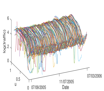
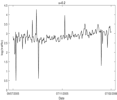
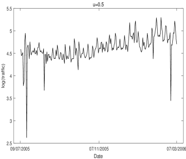
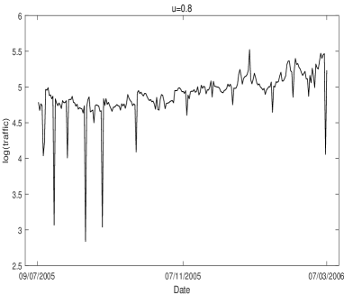
Figure 1: (a): 3D Transformed functional time series plot. (b): Transformed time series plot for fixed $u=0.2$. (c): Transformed time series plot for fixed $u=0.5$. (d): Transformed time series plot for fixed $u=0.8$.

The aim of this article is to build a theoretical foundation as well as to provide an efficient methodology for the optimal short-term linear forecasting of locally stationary functional time series. Here local stationarity refers to a smoothly or slowly time-varying data generating mechanism. Our work is motivated by a curve forecasting problem for telecommunication network traffic data. Specifically, the data set consists of user download data for a mobile infrastructure network deployed in Asia and the United States recorded minutely for a period of roughly 8 months. Though the data are recorded at a high frequency, engineers and administrators are interested in forecasting the download pattern of a future day or several days in hope of promoting efficient operation of the network system. To this end and due to the strong daily periodicity of the data, a typical way is to transform the observed data on day $i$, $Y_{i}(u_{j})$, $i=1,...,n$ into smooth daily curves $Y_{i}(u)$ for $u\in[0,1]$ (refer to Fig. 1(a) for the logarithm transformed daily curves), where $u_{j}=j/1440$, $j=1,2,\cdots,1440$ denotes the $j$th minute of the day. Then one seeks to predict the future curves of downloads $Y_{n+k}(u),~{}k\geq 1$.

One of the most significant characteristics of the telecommunication network traffic time series lies in its non-stationarity. For instance, take a look at the log-transformed time series at $u=0.2,0.5$ and $0.8$ respectively in Fig. 1(b)–(d). It is clear that there exists an upward trend and obvious changes of variability over time, contributing to the non-stationarity of the functional data.

Building a unified theoretical foundation for locally stationary functional time series prediction is difficult due to the lack of insights into the structure of the series. For a univariate and weakly stationary time series, the Wiener-Kolmogorov prediction theory ([32, 49]) elucidates that it can be represented as a white-noise-driven auto-regressive (AR) process of infinite order under some mild conditions. Recently, Ding and Zhou [15] established a unified AR approximation theory for a wide class of univariate non-stationary time series under some mild conditions. Nevertheless, it has been a difficult and open problem to build structural representations or approximations for functional time series since the intrinsic infinite-dimensional nature of such processes brings great technical difficulty to studying the structure of such complex dynamic systems. In particular, the covariance operator of a smooth functional time series is not invertible which makes it difficult to extend the existing linear approximation theory of univariate and fixed-dimensional multivariate time series directly to the functional setting.

Our major theoretical contribution in this paper lies in establishing a functional AR approximation theory for a rich class of locally stationary functional time series. To be more specific, we prove that a wide class of short memory locally stationary functional time series can be well approximated by a locally stationary white-noise-driven functional AR process of slowly diverging order, see Theorem 1 for a more precise statement. The construction of this structural approximation relies on a sieve truncation technique, the modern operator spectral theory, and the classic approximation theory which transfers the infinite-dimensional problem into a high-dimensional one and subsequently controls the decay rates of the inverse of high-dimensional banded matrices. To our best knowledge, there is no such structural approximation result in the field of functional data analysis, even under stationary scenarios. As a fundamental theory, our functional AR approximation result sheds light on the underlying linear structure of a wide class of functional time series and hence serves as a unified foundation for an optimal linear forecasting theory of such processes. Furthermore, the functional AR approximation theory could have a much wider range of applications in various fundamental problems in functional time series analysis such as covariance inference, adaptive resampling, efficient estimation, and dependence quantification.

The functional AR approximation theory is nonparametric in nature and it provides a more flexible and robust way to forecast a rich class of locally stationary functional time series without resorting to restrictive parametric modeling of the covariance operator compared to existing methods built on parametric linear time series models. Methodologically, we propose a nonparametric double-sieve method for the estimation of the AR coefficient functions where sieve expansions are conducted and then truncated over both the function and time domains. Unlike most non-stationary time series forecasting methods in the literature where only data near the end of the sequence are utilized for the forecast ([14, 39]), the nonparametric sieve regression used in our prediction is global in the sense that it utilizes all available functional curves to determine the optimal forecast coefficients and hence is expected to be more efficient. Due to the adaptivity of the double-sieve expansion, we also claim that the prediction errors are adaptive to the smoothness of the functional time series and the strength of the temporal dependence (c.f. Theorem 3).

There is substantial literature on prediction techniques and theory for stationary functional time series, most of which were essentially built on linear functional time series assumptions but without investigating whether the functional time series of interest can be represented or approximated by a linear model. Bosq [6] suggested a one-step ahead prediction based on the functional AR process. Hyndman and Ullah [26] introduced a robust forecasting approach where principal component scores were predicted via a univariate time series forecasting method. As an extension of the latter, Aue et al. [2] proposed a forecasting method based on vector auto-regressive forecasts of principal component scores. Later, Aue et al. [1] considered the functional moving average (FMA) process and introduced an innovation algorithm to obtain the best linear predictor. The vector auto-regressive moving average (VARMA) model was investigated by [27] for modeling and forecasting principal component scores. Other available methods for forecasting include functional kernel regression ([16]), functional partial least squares regression ([38]), dynamic updating approaches for incomplete trajectories ([44]), and robust forecasting method via dynamic functional principal component regression for data contaminated by outliers ([43]).

Meanwhile, the last two decades have witnessed some developments in prediction for locally stationary time series; see for instance [13, 14, 15, 17, 39]. However, studies on locally stationary functional time series remain scarce. Recently, Van Delft and Eichler [46] discussed inference and forecasting methods for a class of time-varying functional processes based on auto-regressive fitting. Kurisu [33] investigated the estimation of locally stationary functional time series and applied it to $k$-step ahead prediction using a kernel-based method.

The remainder of this paper is organized as follows. In Section 2, we establish the functional AR approximation result under some mild assumptions. Section 3 provides one application of our theory in optimal forecasting of locally stationary functional time series. Practical implementation including the selection for tuning parameters and optimal prediction algorithm are discussed in Section 4. Section 5 reports some supporting Monte Carlo simulation experiments. A real data application for the prediction of daily telecommunication downloads is carried out in Section 6. Additional results and technical proofs are deferred to the Appendix.

2 Functional AR approximation to locally stationary functional time series

Throughout this paper, let $\mathcal{L}^{2}([0,1])$ be a separable Hilbert space of all square integrable functions on $[0,1]$ with inner product $\langle x,y\rangle=\int_{0}^{1}x(u)y(u)\mathrm{d}u$. A square integrable random function $Y(u)\in\mathcal{L}^{2}[0,1]$ implies $\mathbb{E}|Y(u)|_{\mathcal{L}^{2}}^{2}<\infty$, where $|Y(u)|_{\mathcal{L}^{2}}^{2}=\int_{0}^{1}Y^{2}(u)\mathrm{d}u$ signifies its $\mathcal{L}^{2}$ norm. We also denote by $\mathcal{C}^{d}([0,1])$ the collection of functions that are $d$-times continuously differentiable with absolutely continuous $d$-th derivative on $[0,1]$. For a random variable $Z$ and some constant $q>1$, denote by $\|Z\|_{q}=(\mathbb{E}|Z|^{q})^{1/q}$ its $L^{q}$ norm. The notation $\|\cdot\|$ signifies the operator norm (i.e., largest singular value) when applied to matrices and the Euclidean norm when applied to vectors. If $f(x)\asymp g(x)$, we say that functions $f(x)$ and $g(x)$ have the same order of magnitude. Also, we use $\lambda_{\min}(\cdot)$ and $\lambda_{\max}(\cdot)$ to signify the largest and smallest eigenvalues of matrices. Throughout this paper, the symbol $C$ denotes a generic finite constant that is independent of $n$ and may vary from place to place.

2.1 Locally stationary functional time series

In this subsection, we will first introduce the definition of locally stationary functional time series as follows.

Definition 1 (Locally stationary functional time series)

A non-stationary functional time series $\{Y_{i}(u)\}$ is a locally stationary functional time series (in covariance) if there exists a function $\gamma(t,u,v,k):[0,1]^{3}\times\mathbb{Z}\to\mathbb{R}$ such that

$${\rm Cov}(Y_{i}(u),Y_{j}(v))=\gamma(t_{i},u,v,i-j)+\mathcal{O}\left(\frac{|i-j|+1}{n}\right),~{}t_{i}=\frac{i}{n}.$$ (1)

Furthermore, we assume that $\gamma$ is Lipschitz continuous in time $t$ and for any fixed $t\in[0,1]$, $\gamma(t,u,v,\cdot)$ is the autocovariance function of a stationary functional time series.

This definition only imposes a smoothness condition on the covariance structure of $\{Y_{i}(u)\}$ with respect to time. From Eq. 1, we find that the underlying data generating mechanism evolves smoothly over time, which implies that the covariance structure of $\{Y_{i}(u)\}$ in any small time segment can be well approximated by that of a stationary functional process. Definition 1 covers a wide class of frequently used locally stationary functional time series models, and we shall provide an example in the following.

Example 1

Consider the following locally stationary functional time series

$$Y_{i}(u)=H(\frac{i}{n},u,\mathcal{F}_{i}),$$ (2)

where $\mathcal{F}_{i}=(\cdots,\eta_{i-1},\eta_{i})$ with $\eta_{i}$ being i.i.d. random elements and $H:[0,1]^{2}\times\mathbb{R}^{\infty}\to\mathbb{R}$ is a measurable function such that $\xi_{i}(t,u):=H(t,u,\mathcal{F}_{i})$ is a properly defined random function in $\mathcal{L}^{2}$. Furthermore, the following assumption is needed to ensure local stationarity.

Assumption 1

$H(t,\cdot,\cdot)$ defined in (2) satisfies the stochastic Lipschitz continuous condition across $t$, that is for some $q>2$ and any $u\in[0,1]$,

$$\|H(t_{1},u,\mathcal{F}_{i})-H(t_{2},u,\mathcal{F}_{i})\|_{q}\leq C|t_{1}-t_{2}|,$$ (3)

where $C>0$ and $t_{1},t_{2}\in[0,1]$. Moreover, we assume

$$\sup_{t,u\in[0,1]}\|H(t,u,\mathcal{F}_{i})\|_{q}<\infty.$$ (4)

In this context, the autocovariance function $\gamma(t,u,v,j)$, $j\in\mathbb{Z}$ in Definition 1 can be represented as

$$\gamma(t,u,v,j)={\rm Cov}(H(t,u,\mathcal{F}_{0}),H(t,v,\mathcal{F}_{j})).$$ (5)

Under 1, this type of locally stationary functional process in (2) satisfies Definition 1. See Lemma 1 in Section B of the Supplementary Material for detailed proof.

Till the end of the paper, we consider a locally stationary functional time series $\{Y_{i}(u)\}_{i=1}^{n}\in\mathcal{L}^{2}([0,1])$ satisfying Definition 1 and $\mathbb{E}|Y_{i}(u)|_{\mathcal{L}^{2}}^{2}<\infty$, then it can always be decomposed as

$$Y_{i}(u)=\mu_{i}(u)+Z_{i}(u),~{}i=1,...,n,$$

where $\mu_{i}(u)=\mathbb{E}(Y_{i}(u)),~{}u\in[0,1]$ is the mean function and $Z_{i}(u)$ is the centered locally stationary functional process in $\mathcal{L}^{2}([0,1])$. For simplicity, we assume that $\mu_{i}(u)=0$. Let $\{\alpha_{k}(u)\}_{k=1}^{\infty}$ be a set of pre-determined orthonormal basis functions on $\mathcal{L}^{2}([0,1])$, the functional time series $Y_{i}(u)$ admits the following Karhunen-Loève type expansion

$$Y_{i}(u)=\sum_{k=1}^{\infty}r_{i,k}\alpha_{k}(u)=\sum_{k=1}^{\infty}x_{i,k}f_{k}\alpha_{k}(u),$$ (6)

where $r_{i,k}=\int_{0}^{1}Y_{i}(u)\alpha_{k}(u)\mathrm{d}u$ is the $k$th (random) basis expansion coefficient of $Y_{i}(u)$ with respect to $\{\alpha_{k}(u)\}_{k=1}^{\infty}$. For examples of commonly used basis functions, we refer readers to Section A in the Supplementary Material. In (6), $f_{k}^{2}$ is the asymptotically average variance of $r_{i,k}$ over $i$, denoted by $f_{k}^{2}:=\int_{T^{3}}\gamma(t,u,v,0)\alpha_{k}(u)\alpha_{k}(v)\mathrm{d}u\mathrm{d}v\mathrm{d}t$, $T=[0,1]$. $f_{k}$ captures the average magnitude of $r_{i,k}$ and it decays as $k$ increases. If $f_{k}\neq 0$, then $\{x_{i,k}:=r_{i,k}/f_{k}\}_{i=1}^{n}$ is a locally stationary (scalar) time series for any $k\geq 1$. Observe that the magnitude of $x_{i,k}$ is expected to be stable as $k$ increases.

It is worth noting that in the stationary context, one often uses $f_{k}:={\rm Std}(r_{i,k})$ to describe the decay speed of $r_{i,k}$ as $k$ increases and the latter representation is frequently used in the functional data analysis literature; see for instance [42] and [12]. Our definition of $f_{k}$ can be viewed as the corresponding extension to the locally stationary setting. The following assumption restricts the decay speed of the basis expansion coefficient $r_{i,k}$.

Assumption 2

We assume that the functional time series $Y_{i}(u)\in\mathcal{C}^{d_{1}}([0,1])$ a.s., where $d_{1}>0$ is some integer. Furthermore, suppose the random coefficient $r_{i,k}=\mathcal{O}_{\mathbb{P}}(k^{-(d_{1}+1)})$ for $i=1,...,n$.

It is well-known that for a general $\mathcal{C}^{d}([0,1])$ function where $d$ is a non-negative integer, the fastest decay rate for its $k$th basis expansion coefficient is $\mathcal{O}(k^{-(d+1)})$ for a wide class of basis functions ([9]). For example, the Fourier basis (for periodic functions), the weighted Chebyshev polynomials ([45]) and the orthogonal wavelets with degree $m\geq d$ ([35]) admit the latter decay rate under some extra mild assumptions on the behavior of the function’s $d$th derivative. On the other hand, the basis expansion coefficients may decay at slower speeds for some orthonormal bases. An example is the normalized Legendre polynomials basis function where the coefficients decay at an $\mathcal{O}(k^{-(d+1/2)})$ speed ([48]). We remark that our functional AR approximation result can be achieved for basis functions whose corresponding coefficients decay at slower rates with the bound error slightly larger but still converging to zero under mild conditions. For the sake of brevity, we shall stick to the fastest decay 2 for our theoretical investigations throughout this paper.

2.2 Functional AR approximation theory

Here, we will establish a functional AR approximation theory for locally stationary functional time series. Let $b=b(n)$ be a generic value which specifies the order of functional AR approximation. For theoretical and practical purposes, $b$ is required to be much smaller than the sample size $n$ to achieve a parsimonious approximating model. To explore the theoretical results of the functional AR approximation, we will truncate the infinite representation (6) to finite (but diverging) dimensional spans of basis functions as follows

$$Y_{i}(u)=\sum_{k=1}^{p}x_{i,k}f_{k}\alpha_{k}(u)+\mathcal{O}_{\mathbb{P}}(p^{-d_{1}}):=Y_{i}^{(p)}(u)+\mathcal{O}_{\mathbb{P}}(p^{-d_{1}}),$$ (7)

where $p=p(n)$ is the truncation number. This truncated expansion in (7) serves as the first dimension reduction for our theoretical investigation, which is a common technique in functional time series analysis. For example, with this approach, one could apply the initial dimension reduction by functional principal component analysis ([42, 30]), or explore properties of linear regression estimators ([21, 34]). Some existing work suggests projecting infinite dimensional objects onto a fixed dimensional subspace to facilitate statistical calculations ([2]), that is, the truncation number is a fixed constant. However, there is a growing interest in allowing the truncation number to grow to infinity with the sample size $n$ in order to make the truncation adaptive to the smoothness of the functional observations, see [21, 34]. Throughout this paper, we assume that the truncation number diverges to infinity at a relatively slow speed, i.e., $p\asymp n^{\beta_{1}},\beta_{1}\in(0,1)$. We will discuss how to select it in Section 4.1.

Since the functional time series is centered, we have $\mathbb{E}(x_{i,k})=0$ for any $i=1,...,n,~{}k\geq 1$. When $i>b$, the best linear prediction (in terms of the mean squared prediction error) of $\bm{x}_{i}:=(x_{i,1},...,x_{i,p})^{\top}$ which utilizes all its predecessors $\bm{x}_{1},...,\bm{x}_{i-1}$ can be expressed as

$$\widehat{\bm{x}}_{i}=\sum_{j=1}^{i-1}\bm{\Phi}_{i,j}\bm{x}_{i-j},$$

where $\{\bm{\Phi}_{i,j}\}$ are the prediction coefficient matrices. By construction, $\bm{\epsilon}_{i}:=\bm{x}_{i}-\widehat{\bm{x}}_{i}$ is a white noise process with mean $\bm{0}$ and covariance matrix denoted by $\bm{\Sigma}_{i}$. Furthermore, let $\bm{\Gamma}(t,j)\in\mathbb{R}^{p\times p}$ be the autocovariance matrix of $\bm{x}_{i}$ at some rescaled time $t\in[0,1]$ and lag $j\in\mathbb{Z}$ with $\gamma_{k,l}(t,j)$ being its $(k,l)$th element for $k,l=1,...,p$. Note that $\gamma_{k,l}(t,j)=\int_{T^{2}}\gamma(t,u,v,j)\alpha_{k}(u)\alpha_{l}(v)\mathrm{d}u\mathrm{d}v/(f_{k}f_{l})$ where $\gamma(t,u,v,j)$ is defined in Definition 1. Together with Eq. (1), it also indicates that the covariance structure of the scaled multivariate time series $\{\bm{x}_{i}\}$ can be determined by the covariance of the functional time series $\{Y_{i}(u)\}$. In order to provide a theoretical foundation for the functional AR approximation, certain assumptions are required.

Assumption 3

For any $j\in\mathbb{Z}$, we assume that $\bm{\Gamma}(t,j)\in\mathcal{C}^{d_{2}}([0,1])$, where $d_{2}>0$ is some integer. In other words for any integers $k,l\geq 1$, each component $\gamma_{k,l}(t,j)$ is $d_{2}$ times continuously differentiable with respect to $t$ over $[0,1]$.

Assumption 4

For $j\in\mathbb{Z}$, suppose that $\sup_{t\in[0,1]}\|\bm{\Gamma}(t,j)\|\leq C(|j|+1)^{-\tau}$ for some constant $\tau>1$.

3 is a local stationarity assumption and it imposes a smoothness requirement on the autocovariance matrix $\bm{\Gamma}(t,j)$. Simple calculations show that 4 implies that $\max_{k,l}|{\rm Cov}(x_{i,k},x_{i+j,l})|\leq C(|j|+1)^{-\tau}$, which provides a polynomial decay rate of the covariance structures of random variables. In particular, 4 states that the correlation among components of the random vector $\bm{x}_{i}$ is relatively weak. This condition is generally mild and can be fulfilled in most cases, as the random components $x_{i,k}$ typically exhibit weak dependence between different $k$ under appropriate basis expansions.

Now, we will provide an example of locally stationary multivariate time series.

Example 2

Let $\{\bm{\eta}_{i}\}$ be zero-mean i.i.d. $\mathbb{R}^{p}$ random vectors with its covariance matrix $\|\bm{\Sigma}_{\eta}\|<\infty$. We consider the locally stationary linear process as

$$\bm{x}_{i}=\sum_{m=0}^{\infty}\bm{A}_{m}(t_{i})\bm{\eta}_{i-m},~{}~{}t_{i}=\frac{i}{n},$$

where $\bm{A}_{m}(t)\in\mathbb{R}^{p\times p}$ is assumed to be a $\mathcal{C}^{d_{2}}([0,1])$ function with respect to $t$. Then Assumptions 3 and 4 will be satisfied if

$$\sup_{t\in[0,1]}\left\|\frac{\partial^{d_{2}}\bm{A}_{m}(t)}{\partial t^{d_{2}}}\right\|\leq C(m+1)^{-\tau},~{}~{}\sup_{t\in[0,1]}\|\bm{A}_{m}(t)\|\leq C(m+1)^{-\tau}$$

hold, respectively. We refer readers to Lemma 3 in Section B of the Supplementary Material for detailed proof.

Furthermore, to avoid erratic behavior of the functional AR approximation, the smallest eigenvalue of the covariance matrix of multivariate time series $\{\bm{x}_{i}\}_{i=1}^{n}$ should be bounded away from zero. Similar to the uniformly-positive-definite-in-covariance (UPDC) condition for univariate time series discussed in [15], we put forth an assumption for the multivariate version as follows.

Assumption 5 (UPDC condition for multivariate time series)

Denote $\bm{{\rm x}}=(\bm{x}_{1}^{\top},\\ ...,\bm{x}_{n}^{\top})^{\top}\in\mathbb{R}^{np}$. For all sufficiently large $n\in\mathbb{N}$, there exists a universal constant $\kappa_{1}>0$ such that the smallest eigenvalue of ${\rm Cov}(\bm{{\rm x}})$ is bounded away by $\kappa_{1}$, where ${\rm Cov}(\cdot)$ is the covariance matrix of the given vector.

This condition is necessary to avoid ill-conditioned ${\rm Cov}(\bm{{\rm x}})$ and hence makes the construction of functional AR approximation feasible. Note that it is a mild requirement and has been widely used in the statistical literature for covariance and precision matrix estimation; see for instance, [10], [8] and references therein. When it comes to stationary multivariate time series with short memory, [7, Theorem 11.8.1] states that the UPDC condition holds if its spectral density matrix is uniformly bounded below by a positive constant. To practically verify the UPDC assumption in the case of locally stationary multivariate time series, we provide a necessary and sufficient condition below.

Proposition 1

Suppose that $\{\bm{x}_{i}\}_{i=1}^{n}$ is locally stationary multivariate time series satisfying 4. If there exists some constant $\kappa_{1}>0$ such that the smallest eigenvalue of the spectral density matrix, i.e., $\lambda_{\min}(\bm{f}(t,\omega))\geq\kappa_{1}$ for all $t$ and $\omega\in[-\pi,\pi]$, where

$$\bm{f}(t,\omega)=\frac{1}{2\pi}\sum_{h\in\mathbb{Z}}{\rm e}^{-{\rm i}h\omega}\bm{\Gamma}(t,h),~{}~{}{\rm i}=\sqrt{-1},$$ (8)

then $\{\bm{x}_{i}\}_{i=1}^{n}$ satisfies 5. Conversely, if $\{\bm{x}_{i}\}_{i=1}^{n}$ satisfies Assumptions 4 and 5, then there exists some constant $\kappa_{1}>0$ such that $\lambda_{\min}(\bm{f}(t,\omega))\geq\kappa_{1}$ for all $t$ and $\omega\in[\pi,\pi]$.

Proposition 1 demonstrates that the verification of 5 boils down to checking whether the smallest eigenvalue of the local spectral density matrix $\bm{f}(t,\omega)$ is uniformly bounded from below by some positive constant. Here, we provide an example to check the UPDC condition via Proposition 1.

Example 3

Rewrite the linear process in Example 2 as

$$\bm{x}_{i}=\bm{\mathcal{A}}(\frac{i}{n},B)\bm{\eta}_{i},$$

where $\bm{\mathcal{A}}(\cdot,B)=\sum_{m=0}^{\infty}\bm{A}_{m}(\cdot)B^{m}$ with the backshift operator $B$, and $\{\bm{\eta}_{i}\}$ are zero-mean i.i.d. random vectors with non-degenerate covariance matrix $\bm{\Sigma}_{\eta}$. Using the property of linear filters for the spectral density matrix, we have

$$\bm{f}(t,\omega)=\frac{1}{2\pi}\bm{\mathcal{A}}(t,{\rm e}^{-{\rm i}\omega})\bm{\Sigma}_{\eta}\bm{\mathcal{A}}^{\top}(t,{\rm e}^{{\rm i}\omega}),\quad-\pi\leq\omega\leq\pi.$$

Therefore, by Proposition 1, we can obtain that the UPDC condition is satisfied if

$$\lambda_{\min}(\bm{\mathcal{A}}(t,{\rm e}^{-{\rm i}\omega})\bm{\mathcal{A}}^{\top}(t,{\rm e}^{{\rm i}\omega}))\geq\kappa_{1}>0~{}\text{for~{}all~{}}t~{}\text{and}~{}\omega.$$

The next theorem is our main theoretical result and it provides a functional AR approximation theory under the short-range dependence and local stationarity conditions.

Theorem 1

Consider the locally stationary functional time series from Definition 1. Under Assumptions 2–5 and suppose $\sup_{t\in[0,1]}\left\|\partial\bm{\Gamma}(t,j)/\partial t\right\|\leq C$ for all $j\in\mathbb{Z}$. Then we obtain that for $i\geq 2$,

$$Y_{i}(u)=\sum_{j=1}^{\min\{i-1,b\}}\int_{0}^{1}\psi_{j}^{(p)}(\frac{i}{n},u,v)Y_{i-j}(v)\mathrm{d}v+\varepsilon_{i}(u)+\mathcal{O}_{\mathbb{P}}\left(p^{1/2}b^{-\tau+2}(\log b)^{\tau-1}+\frac{p^{1/2}b^{3}}{n}+p^{-d_{1}}\right),$$ (9)

where $\psi_{j}^{(p)}(\cdot,u,v)\in\mathcal{L}^{2}([0,1]^{2})$ admits the basis expansion $\psi_{j}^{(p)}(t,u,v):=\sum_{k,l=1}^{p}\psi_{j,kl}(t)\alpha_{k}(u)\alpha_{l}(v)$ with the coefficient $\psi_{j,kl}(t)\in\mathcal{C}^{d_{2}}([0,1])$ with respect to $t$ for all $j$, and the error process $\epsilon_{i}(u):=\bm{\alpha}_{f}^{\top}(u)\bm{\epsilon}_{i}$ is a functional white noise process, where $\bm{\alpha}_{f}(u)=(\alpha_{1}(u)f_{1},...,\alpha_{p}(u)f_{p})^{\top}$.

Theorem 1 states that a wide class of locally stationary functional time series can be efficiently approximated by a locally stationary functional autoregressive process with smoothly time-varying operators (kernels) and a slowly diverging order $b$. Notice that the functional AR coefficient function $\psi_{j}^{(p)}(t,u,v)$ has the same degree of smoothness over time $t$ as the time-varying covariance functions $\bm{\Gamma}(t,j)$ specified in 3. In addition, the first and second error terms on the right-hand side of (9) describe the functional AR approximation errors based on $Y_{i}^{(p)}(u)$, and the third term reflects the truncation error due to (7). The approximation result in (9) also reveals that the error bound is adaptive to the smoothness of the functional observations ($d_{1}$), as well as the temporal dependence structure of $\{Y_{i}(u)\}$ ($\tau$). In particular, the optimal choice of the AR order $b$ can be obtained by balancing the first two error terms in (9). Simple calculations yield that the optimal $b\asymp n^{\frac{1}{\tau+1}}(\log n)^{\theta}$ with $\theta=\frac{\tau-1}{\tau+1}$. Similarly, the optimal choice for the truncation number $p\asymp n^{\frac{\tau-2}{(\tau+1)(d_{1}+1/2)}}(\log n)^{\frac{-3\theta}{d_{1}+1/2}}$, and minimum AR approximation error turns out to be $\mathcal{O}\Big{(}n^{-\frac{d_{1}(\tau-2)}{(\tau+1)(d_{1}+1/2)}}(\log n)^{\frac{3d_{1}\theta}{d_{1}+1/2}}\Big{)}$. For example, when the functions are infinite many times differentiable, that is $d_{1}\rightarrow\infty$, we have that the minimum approximation error in (9) becomes $\mathcal{O}\Big{(}n^{-\frac{\tau-2}{\tau+1}}(\log n)^{3\theta}\Big{)}$.

We will conclude this subsection by extending the functional AR approximation result to the case when the temporal dependence is of exponential decay in the following statement.

Remark 1

When the temporal dependence of the covariance structure in 4 is changed to exponential decay, i.e., $\sup_{t\in[0,1]}\|\bm{\Gamma}(t,j)\|\leq C\rho^{|j|}$ with $\rho\in(0,1)$, then the optimal choice of $b\asymp\log n$. Consequently, the functional AR approximation result (9) in Theorem 1 will be updated to

$$Y_{i}(u)=\sum_{j=1}^{\min\{i-1,b\}}\int_{0}^{1}\psi_{j}^{(p)}(\frac{i}{n},u,v)Y_{i-j}(v)\mathrm{d}v+\varepsilon_{i}(u)+\mathcal{O}_{\mathbb{P}}\left(\frac{p^{1/2}\log^{3}n}{n}+p^{-d_{1}}\right).$$

In this case, the optimal choice for the truncation number $p\asymp n^{\frac{2}{2d_{1}+1}}(\log n)^{-\frac{6}{2d_{1}+1}}$ and the error term turns out to be $\mathcal{O}_{\mathbb{P}}\Big{(}n^{-\frac{2d_{1}}{2d_{1}+1}}(\log n)^{\frac{6d_{1}}{2d_{1}+1}}\Big{)}$.

3 Applications to optimal short-term forecast for locally stationary functional time series

In this section, we will discuss the application of our functional AR approximation theory to optimal short-term forecasting for locally stationary functional time series. Generally speaking, Theorem 1 provides a theoretical guarantee for the optimal short-term linear forecasting of a short-memory locally stationary functional time series by a locally stationary functional AR process of slowly diverging order. Section 3.1 will discuss the details. Provided that the underlying data generating mechanism is sufficiently smooth and the temporal dependence is sufficiently weak, the unknown coefficients $\psi_{j,kl}(t)$ in the basis expansion of $\psi_{j}^{(p)}(t,u,v)$ can be consistently estimated via a Vector Auto-Regressive (VAR) approximation and the method of sieves, which will be implemented in Section 3.2 and Section 3.3.

3.1 Optimal functional time series prediction

In this paper, we shall focus on the best continuous linear prediction of functional time series; that is, given $i\geq 2$ and $Y_{1}(u),\cdots,Y_{i-1}(u)$, we try to find a linear predictor $\widehat{Y}_{i}(u)$ of $Y_{i}(u)$ in the form

$$\widehat{Y}_{i}(u)=\sum_{j=1}^{i-1}\int_{0}^{1}g_{i,j}(u,v)Y_{i-j}(v)\mathrm{d}v$$ (10)

such that $\mathbb{E}|Y_{i}(u)-\widehat{Y}_{i}(u)|_{\mathcal{L}^{2}}^{2}$ is minimized, where the kernel function $g_{i,j}(u,v)\in\mathcal{L}([0,1]^{2})$ is continuous over $u$ and $v$ for all $i$ and $j$. The goal of this subsection is to investigate the optimal short-term continuous prediction of locally stationary functional time series $\{Y_{i}(u)\}_{i=1}^{n}$.

To begin with, we consider the truncated process $\{Y_{i}^{(p)}(u)\}_{i=1}^{n}$ defined in (7) and let the best linear predictor of $Y_{i}^{(p)}(u)$ in terms of $Y_{1}^{(p)}(u),\cdots,Y_{i-1}^{(p)}(u)$ be $\widehat{Y}_{i}^{(p)}(u)$. The next theorem shows the asymptotic equivalence of the best continuous linear predictor $\widehat{Y}_{n+1}(u)$ and $\widehat{Y}_{n+1}^{(p)}(u)$.

Theorem 2

Define prediction errors as ${\rm PE}_{n+1}=Y_{n+1}(u)-\widehat{Y}_{n+1}(u)$ and ${\rm PE}_{n+1}^{(p)}=Y_{n+1}^{(p)}(u)-\widehat{Y}_{n+1}^{(p)}(u)$. Suppose Assumptions 2 and 4 hold, then we obtain

$$\mathbb{E}|{\rm PE}_{n+1}|_{\mathcal{L}^{2}}^{2}-\mathbb{E}|{\rm{PE}}_{n+1}^{(p)}|_{\mathcal{L}^{2}}^{2}=\mathcal{O}\left(p^{-(d_{1}+1)}\right).$$

This theorem illustrates that, by the fact that $Y_{n+1}(u)=Y_{n+1}^{(p)}(u)+\mathcal{O}_{\mathbb{P}}(p^{-d_{1}})$ in (7), the best linear predictor $\widehat{Y}_{n+1}^{(p)}(u)$ and the best continuous linear predictor $\widehat{Y}_{n+1}(u)$ are asymptotically equivalent as $p\to\infty$. Next, denote the Auto Regressive (AR) predictor

$$\widetilde{Y}_{i}^{(b)}(u):=\sum_{j=1}^{\min\{i-1,b\}}\int_{0}^{1}\psi_{j}^{(p)}(\frac{i}{n},u,v)Y_{i-j}(v)\mathrm{d}v,$$ (11)

which is the dominating term on the right hand side of (9) of our AR approximation theory. The following theorem states that the best continuous linear predictor $\widehat{Y}_{n+1}(u)$ can be well approximated by the AR predictor $\widetilde{Y}_{n+1}^{(b)}(u)$.

Theorem 3

Denote the prediction error ${\rm PE}_{n+1}^{(b)}:=Y_{n+1}^{(p)}(u)-\widetilde{Y}_{n+1}^{(b)}(u)$. Suppose that Assumptions 2–5 hold and $\sup_{t\in[0,1]}\|\partial\bm{\Gamma}(t,j)/\partial t\|\leq C$ for all $j\in\mathbb{Z}$, we have

$$\mathbb{E}|{\rm PE}_{n+1}|_{\mathcal{L}^{2}}^{2}-\mathbb{E}|{\rm PE}_{n+1}^{(b)}|_{\mathcal{L}^{2}}^{2}=\mathcal{O}\left(p^{-(d_{1}+1)}+pb^{-2\tau+3}(\log b)^{2\tau-3}+pb^{5}/n^{2}\right).$$ (12)

Theorem 3 implies that the error bound on the right hand side of Eq. 12 converges to $0$ as $p,n\to\infty$. Specifically, with the optimal choice of $b\asymp n^{\frac{1}{\tau+1}}(\log n)^{\theta}$ where $\theta=\frac{\tau-3/2}{\tau+1}$, the optimal MSE rate (12) turns out to be $\mathcal{O}\Big{(}n^{-\frac{(d_{1}+1)(2\tau-3)}{(d_{1}+2)(\tau+1)}}(\log n)^{\frac{5\theta(d_{1}+1)}{d_{1}+2}}\Big{)}$ by choosing $p\asymp n^{\frac{2\tau-3}{(d_{1}+2)(\tau+1)}}(\log n)^{-\frac{5\theta}{d_{1}+2}}$. Furthermore, if the smoothness parameter $d_{1}\to\infty$, the rate becomes $\mathcal{O}\left(n^{-2+5/(\tau+1)}(\log n)^{5\theta}\right)$. It consequently indicates that the AR predictor $\widetilde{Y}_{n+1}^{(b)}(u)$ is asymptotically equivalent to the best continuous linear predictor $\widehat{Y}_{n+1}(u)$ when $\tau>3/2$.

Remark 2

Alternatively, if the covariance structure in 4 decays exponentially fast, then one could choose $b\asymp\log n$ and the result in Theorem 3 can be updated as

$$\mathbb{E}|{\rm PE}_{n+1}|_{\mathcal{L}^{2}}^{2}-\mathbb{E}|{\rm PE}_{n+1}^{(b)}|_{\mathcal{L}^{2}}^{2}=\mathcal{O}\left(p^{-(d_{1}+1)}+p(\log n)^{5}/n^{2}\right).$$ (13)

Hence, (13) equals $\mathcal{O}\left(n^{-\frac{2(d_{1}+1)}{d_{1}+2}}(\log n)^{\frac{5(d_{1}+1)}{d_{1}+2}}\right)$ by choosing $p\asymp n^{\frac{2}{d_{1}+2}}(\log n)^{-\frac{5}{d_{1}+2}}$. Similarly, if in addition $d_{1}\to\infty$, then the right hand side of (13) becomes $\mathcal{O}(n^{-2}(\log n)^{5})$.

3.2 Vector Auto-Regressive approximation

With the theoretical results in Section 3.1, it is clear that the short-term forecasting for locally stationary functional time series is equivalent to exploring the optimal short-term continuous linear prediction by a locally stationary functional AR process. On the other hand, we will demonstrate that the unknown coefficients $\psi_{j,kl}(t)$ in the basis expansion of $\psi_{j}^{(p)}(t,u,v)$ in (10) can be determined by the coefficient matrix in a smoothly-varying VAR approximation. Then it turns out that the optimal short-term forecasting problem boils down to that of efficiently estimating the smoothly-varying VAR coefficient matrices at the right boundary. To this end, in this subsection we start with the prediction coefficient matrix $\bm{\Phi}_{i,j}$ defined in Section 2.2 and investigate its estimation.

Consider the time series $\{\bm{x}_{i}\}$ of diverging dimension $p_{n}$ and we establish its VAR approximation. Consider the following best linear predictions:

$$\bm{x}_{i}=\sum_{j=1}^{i-1}\bm{\Phi}_{i,j}\bm{x}_{i-j}+\bm{\epsilon}_{i},~{}i=2,...,n,$$ (14)

where $\bm{\Phi}_{i,j}$ and $\bm{\epsilon}_{i}$ have been defined in Section 2.2. Let $\bm{x}_{i-1}^{(i)}=(\bm{x}_{i-1}^{\top},...,\bm{x}_{1}^{\top})^{\top}\in\mathbb{R}^{(i-1)p}$ be a block vector and $\bm{\Gamma}_{i}={\rm Cov}(\bm{x}_{i-1}^{(i)},\bm{x}_{i-1}^{(i)})\in\mathbb{R}^{(i-1)p\times(i-1)p}$ be the covariance matrix of $\bm{x}_{i-1}^{(i)}$. Similar to the univariate AR approximation result established in [15], we will demonstrate that a rich class of locally stationary multivariate time series $\bm{x}_{i}$ can be well approximated by a VAR($b$) process under some mild conditions.

Now, denote $\bm{\Phi}_{i}=(\bm{\Phi}_{i,1}^{\top},...,\bm{\Phi}_{i,i-1}^{\top})^{\top}\in\mathbb{R}^{(i-1)p\times p}$, then we have the Yule-Walker equation

$$\bm{\Phi}_{i}=\bm{\Omega}_{i}\bm{\gamma}_{i},$$

where $\bm{\Omega}_{i}=\bm{\Gamma}_{i}^{-1}$ and $\bm{\gamma}_{i}={\rm Cov}(\bm{x}_{i-1}^{(i)},\bm{x}_{i})\in\mathbb{R}^{(i-1)p\times p}$. See [7, Section 11.3] for more details on Yule-Walker equation for multivariate time series. We shall first state the following results regarding the coefficient matrices $\bm{\Phi}_{i,j}$.

Proposition 2

Under Assumptions 4 and 5, then for VAR process (14), there exists some constant $C>0$ such that

$$\max_{i}\|\bm{\Phi}_{i,j}\|\leq C\left(\frac{j}{\log j+1}\right)^{-\tau+1},~{}~{}\text{for}~{}~{}j\geq 1.$$ (15)

Proposition 2 provides a polynomial decay rate of the coefficient matrices $\bm{\Phi}_{i,j}$ in (15) when $\tau>1$.

Next, define $\bm{\Phi}^{(b)}(t)=(\bm{\Phi}_{1}^{\top}(t),...,\bm{\Phi}_{b}^{\top}(t))^{\top}\in\mathbb{R}^{bp\times p}$ via the Yule-Walker equation

$$\bm{\Phi}^{(b)}(t)=\bm{\Gamma}_{n}^{-1}(t)\bm{\gamma}_{n}(t),$$

where $\bm{\Gamma}_{n}(t)\in\mathbb{R}^{bp\times bp}$ with its $(i,i+j)$th block matrix as $\bm{\Gamma}(t,j)$ for $j=0,\pm 1,...,\pm(b-1)$ and $\bm{\gamma}_{n}(t)=(\bm{\Gamma}^{\top}(t,1),\cdots,\bm{\Gamma}^{\top}(t,b))^{\top}\in\mathbb{R}^{bp\times p}$. It is worth mentioning that there exists a one-to-one mapping from the coefficient matrix $\bm{\Phi}_{j}(t)$ to the coefficient function $\psi_{j}^{(p)}(t,u,v)$ for $j=1,...,b$ in light of the fact that $\psi_{j}^{(p)}(t,u,v)=\bm{\alpha}_{f}^{\top}(u){\rm diag}(f_{1},\cdots,f_{p})\bm{\Phi}_{j}(t)\\ {\rm diag}(1/f_{1},\cdots,1/f_{p})\bm{\alpha}_{f}(v)$ where $\bm{\alpha}_{f}(\cdot)$ is defined in Theorem 1, and we refer readers to find out more details in the proof of Theorem 1 in Section C.1 of the Supplementary Material. Next proposition implies that the coefficient matrix $\bm{\Phi}_{i,j}$ can be well approximated by the smooth function $\bm{\Phi}_{j}(\frac{i}{n})$ when $i>b$ and $1\leq j\leq b$.

Proposition 3

Under Assumptions 3–5, for any $j=1,...,b$, we have $\bm{\Phi}_{j}(t)=\{\Phi_{j,kl}(t)\}_{k,l=1}^{p}\\ \in\mathcal{C}^{d_{2}}([0,1])$, that is each entry of $\bm{\Phi}_{j}(t)$ is $d_{2}$ times continuously differentiable over $[0,1]$. Furthermore suppose $\sup_{t\in[0,1]}\|\partial\bm{\Gamma}(t,j)/\partial t\|\leq C$ for all $j\in\mathbb{Z}$ holds true, then there exists some constant $C>0$, such that for all $j=1,...,b$,

$$\max_{i>b}\left\|\bm{\Phi}_{i,j}-\bm{\Phi}_{j}\left(\frac{i}{n}\right)\right\|\leq C\left(b^{-\tau+1}(\log b)^{\tau-1}+\frac{b^{2}}{n}\right).$$ (16)

The first term on the right hand side of (16) is the truncation error by using VAR$(b)$ process to approximate the VAR$(i-1)$, which is also the error rate in Lemma 6 in Section C.2 of the Supplementary Material. The second part is the error caused by using the smooth VAR coefficient matrices $\bm{\Phi}_{j}(\cdot)$ to approximate $\bm{\Phi}_{i,j}$ for all $j=1,...,b$.

Combing Propositions 2 and 3, we can rewrite (14) as

$$\left\|\bm{x}_{i}-\sum_{j=1}^{\min\{i-1,b\}}\bm{\Phi}_{j}(\frac{i}{n})\bm{x}_{i-j}-\bm{\epsilon}_{i}\right\|=\mathcal{O}_{\mathbb{P}}\left(p^{1/2}b^{-\tau+2}(\log b)^{\tau-1}+\frac{p^{1/2}b^{3}}{n}\right),~{}i\geq 2.$$ (17)

This formula indicates that the multivariate time series $\bm{x}_{i}$ can be approximated by a locally stationary VAR$(b)$ process with smoothly time-varying coefficients as long as the error terms on the right-hand side of (17) vanish as $n\to\infty$.

3.3 Sieve estimation for coefficient matrices

Based on our discussions in Sections 3.1 and 3.2, optimal prediction of locally stationary functional time series boils down to efficient estimation of the matrix functions $\bm{\Phi}_{j}(\cdot)$, $j=1,2,\cdots b$. This subsection is devoted to the estimation of such matrix coefficient functions. Observe that the smoothness of $\bm{\Phi}_{j}(t)$ over $t$ (c.f. Proposition 3) allows us to conduct another basis expansion and thus estimate them via the method of sieves. Employing the method of sieves on the time-varying coefficient matrices can effectively reduce the dimension of the parameter space in the sense that one only needs to perform a multiple linear regression with a slowly diverging number of predictors. Prior to utilizing this method, we need an assumption concerning the derivatives of $\bm{\Phi}_{j}(t)$.

Assumption 6

The derivatives of $\bm{\Gamma}(t,j)$ over $t$ decay with $|j|$ as follows

$$\sup_{t\in[0,1]}\sum_{j\in\mathbb{Z}}\left\|\frac{\partial^{d_{2}}\bm{\Gamma}(t,j)}{\partial t^{d_{2}}}\right\|<\infty.$$

We mention that 6 entails that all derivatives of $\bm{\Gamma}(t,j)$ over $t$ up to the order $d_{2}+1$ decay as $|j|$ increases. For the linear process in Example 2, this condition will be satisfied if $\sup_{t\in[0,1]}\|\partial^{d_{2}}\bm{A}_{m}(t)\big{/}\partial t^{d_{2}}\|\leq C(m+1)^{-\tau}$. See Lemma 3 of the Supplementary Material for detailed proof. Armed with the relation $\bm{\Phi}_{j}(t)=\bm{E}_{j}^{\top}\bm{\Omega}_{n}(t)\bm{\gamma}_{n}(t)$ where $\bm{E}_{j}^{\top}\in\mathbb{R}^{p\times bp}$ has $\bm{I}_{p}$ at its $j$th block and $\bm{0}_{p}$ at others, the general Leibniz rule as well as the implicit differentiation, it also guarantees that the $d_{2}$th derivative of $\bm{\Phi}_{j}(t)$ over $t$ is bounded ([9, Section 2.3.1]), so that $\bm{\Phi}_{j}(\cdot)$ can be approximated by linear sieves.

Let $\Phi_{j}^{(lm)}(\frac{i}{n})$ be the $(l,m)$th element of coefficient matrix $\bm{\Phi}_{j}(\frac{i}{n})$ for $l,m=1,...,p$. By [9, Section 2.3] and 6, we have that for any $j=1,...,b$,

$$\Phi_{j}^{(lm)}\left(\frac{i}{n}\right)=\sum_{k=1}^{c}\phi_{jk}^{(lm)}v_{k}(\frac{i}{n})+\mathcal{O}(c^{-d_{2}}),~{}i>b,$$ (18)

where $\phi_{jk}^{(lm)}$ for $j=1,...,b$ and $k=1,...,c$ is the $(l,m)$th element in the coefficient matrix $\bm{\phi}_{jk}$, $\{v_{k}(\cdot)\}$ is also a set of pre-chosen orthogonal basis functions on $[0,1]$ and $c=c(n)$ is the truncation number of basis functions. Notice that the first basis expansion in (7) and the second basis expansion in (18) constitute our methodology of double-sieve expansion. Furthermore, let $\bm{z}_{kj}(\frac{i}{n}):=v_{k}(\frac{i}{n})\bm{x}_{i-j}$ and similar to (17), we have for $i=b+1,...,n$,

$$\left\|\bm{x}_{i}-\sum_{j=1}^{b}\sum_{k=1}^{c}\bm{\phi}_{jk}\bm{z}_{kj}\left(\frac{i}{n}\right)-\bm{\epsilon}_{i}\right\|=\mathcal{O}_{\mathbb{P}}\left(p^{1/2}b^{-\tau+2}(\log b)^{\tau-1}+\frac{p^{1/2}b^{3}}{n}+b^{1/2}pc^{-d_{2}}\right).$$ (19)

As a result, the estimation of unknown parameter $\bm{\phi}_{jk}$ boils down to dealing with the above multiple linear regression problem (19). Equipped with the method of double-sieve expansion and the VAR approximation (19), one can consequently estimate the functional AR coefficient as described in (9). In order to facilitate the estimation of coefficient matrix $\bm{\phi}_{jk}$, we impose a regularity condition.

Assumption 7

For any $j=1,...,b$, denote $\bm{W}^{(j)}(t)\in\mathbb{R}^{jp\times jp}$ with its $(k,l)$th block entry $\bm{W}_{kl}^{(j)}(t)=\bm{\Gamma}(t,k-l)\in\mathbb{R}^{p\times p}$ for $k,l=1,...,j$. We assume that the eigenvalues of

$$\int_{0}^{1}\bm{W}^{(j)}(t)\otimes(\bm{v}(t)\bm{v}^{\top}(t))~{}\mathrm{d}t$$

are bounded above and below from zero by a constant $\kappa_{2}>0$, where $\bm{v}(t)=(v_{1}(t),...,v_{c}(t))^{\top}\in\mathbb{R}^{c}$.

Since $\bm{W}^{(j)}(t)\otimes(\bm{v}(t)\bm{v}^{\top}(t))$ is positive semi-definite for all $t\in[0,1]$, the above integral is always positive semi-definite. This assumption is mild and it is easy to check that when $\bm{x}_{i}$ is a stationary process with weak inter-element dependence, the above assumption will hold immediately by UPDC condition and the orthonormality of the basis functions. Moreover, this condition guarantees the invertibility of the design matrix $\bm{Y}$ in the following equation (20) and the existence of the least squares solution.

In this context, denote by $\bm{\beta}$ the $bcp\times p$ block matrix with block rectangular element $\{\bm{\beta}_{j}\}_{j=1}^{b}\in\mathbb{R}^{cp\times p}$, where $\bm{\beta}_{j}=(\bm{\phi}_{j1},...,\bm{\phi}_{jc})^{\top}$. Let $s=1,...,bc,~{}j_{s}=\lfloor{\frac{s-1}{c}}\rfloor+1$ and $k_{s}=s-\lfloor{\frac{s-1}{c}}\rfloor\times c$, then we can define $\bm{y}_{i}\in\mathbb{R}^{bcp}$ by letting its block vector $\bm{y}_{is}=\bm{z}_{k_{s},j_{s}}(\frac{i}{n})$. Moreover, let $\bm{Y}^{\top}$ be the $bcp\times(n-b)$ rectangular matrix whose columns are $\{\bm{y}_{i}\}_{i=b+1}^{n}$ and we also denote $\bm{x}=(\bm{x}_{b+1},...,\bm{x}_{n})^{\top}\in\mathbb{R}^{(n-b)\times p},~{}\bm{\epsilon}=(\bm{\epsilon}_{b+1},...,\bm{\epsilon}_{n})^{\top}\in\mathbb{R}^{(n-b)\times p}$. Then the matrix form of the multiple linear regression for (19) can be constructed as

$$\bm{x}=\bm{Y}\bm{\beta}+\bm{\epsilon}+\bm{Q}_{1}+\bm{Q}_{2},$$ (20)

where

$$\bm{Q}_{1} =\left(\sum_{j=1}^{b}\left[\bm{\Phi}_{b+1,j}-\bm{\Phi}_{j}(\frac{b+1}{n})\right]\bm{x}_{b+1-j},\cdots,\sum_{j=1}^{b}\left[\bm{\Phi}_{n,j}-\bm{\Phi}_{j}(1)\right]\bm{x}_{n-j}\right)^{\top},$$

$$\bm{Q}_{2} =\left(\sum_{j=1}^{b}\sum_{k=c+1}^{\infty}\bm{\phi}_{jk}\bm{z}_{kj}(\frac{b+1}{n}),\sum_{j=1}^{b}\sum_{k=c+1}^{\infty}\bm{\phi}_{jk}\bm{z}_{kj}(\frac{b+2}{n})+\bm{\Phi}_{b+2,b+1}\bm{x}_{1},\cdots,\sum_{j=1}^{b}\sum_{k=c+1}^{\infty}\bm{\phi}_{jk}\bm{z}_{kj}(1)+\sum_{j=b+1}^{n-1}\bm{\Phi}_{n,j}\bm{x}_{n-j}\right)^{\top}.$$

According to the proof of Proposition 4 in Section C.2 of the Supplementary Material, we find that the error terms $\bm{Q}_{1},\bm{Q}_{2}$ are negligible in the regression (20), then by the multiple least squares method, we have

$$\widehat{\bm{\beta}}=(\bm{Y}^{\top}\bm{Y})^{-1}\bm{Y}^{\top}\bm{x}\approx\bm{\beta}+(\bm{Y}^{\top}\bm{Y})^{-1}\bm{Y}^{\top}\bm{\epsilon}.$$

Similarly, one can decompose the estimator $\widehat{\bm{\beta}}$ into its block elements, denoted by $\{\widehat{\bm{\beta}}_{j}\}_{j=1}^{b}\in\mathbb{R}^{cp\times p}$. Hence, the estimate of the time-varying coefficient matrix in (17) can be represented as

$$\widehat{\bm{\Phi}}_{j}(\frac{i}{n})=\widehat{\bm{\beta}}_{j}^{\top}\bm{A}(\frac{i}{n})\quad\text{with}~{}\bm{A}(\cdot)=(v_{1}(\cdot)\bm{\mathrm{I}}_{p},...,v_{c}(\cdot)\bm{\mathrm{I}}_{p})^{\top}\in\mathbb{R}^{cp\times p}.$$ (21)

The rest of this subsection is devoted to the investigation of the convergence rate of $\widehat{\bm{\Phi}}_{j}(\cdot)$. We consider the difference

$$\widehat{\bm{\Phi}}_{j}\left(\frac{i}{n}\right)-\bm{\Phi}_{j}\left(\frac{i}{n}\right)=(\widehat{\bm{\beta}}_{j}-\bm{\beta}_{j})^{\top}\bm{A}\left(\frac{i}{n}\right)-\bm{\Delta}_{c},$$ (22)

where $\bm{\Delta}_{c}$ is a $p\times p$ matrix with its $(l,m)$th entry being $\sum_{k=c+1}^{\infty}\phi_{j,k}^{(lm)}v_{k}(\frac{i}{n})$. Till the end of this paper, we assume $c=\mathcal{O}(n^{\nu_{1}})$ and denote $\zeta_{c}:=\sup_{t}\|\bm{v}(t)\|$ where $\bm{v}(\cdot)$ is defined in 7. Several additional assumptions are needed. First from Eq. 2 and the basis expansion in Eq. 6, we assume that $\{\bm{x}_{i}\}$ admits a physical representation

$$\bm{x}_{i}=\bm{G}(\frac{i}{n},\mathcal{F}_{i}),$$ (23)

where $\bm{G}=(G_{1},...,G_{p})^{\top}$ is a measurable function similar to $H$ defined in (2). The representation form (23) includes many commonly used locally stationary time series models, see for [4, 51] for examples. Consequently, the the $k$th entrywise of $\bm{x}_{i}$ can be written as $x_{i,k}=G_{k}(\frac{i}{n},\mathcal{F}_{i})$. Under the above physical representation, we define the physical dependence measure for the functional time series $\{Y_{i}(u)\}$ with respect to the basis $\{\alpha_{k}(u)\}_{k=1}^{\infty}$ as

$$\delta_{x}(l,q)=\sup_{t\in[0,1]}\max_{1\leq k\leq\infty}\|G_{k}(t,\mathcal{F}_{i})-G_{k}(t,\mathcal{F}_{i,l})\|_{q},~{}l\geq 0,$$ (24)

where $\mathcal{F}_{i,l}=(\mathcal{F}_{i-l-1},\eta_{i-l}^{\ast},\eta_{i-l+1},\cdots,\eta_{i})$ with $\eta_{i-l}^{\ast}$ being an i.i.d. copy of $\eta_{i-l}$.

Assumption 8

There exists some constant $\tau>1$ such that for some constant $C>0$, the physical dependence measure in (24) satisfies $\delta_{x}(l,q)\leq C(l+1)^{-\tau}$ for $l\geq 0$.

Assumption 9

For some constant $C>0$,
(i) there exist $\omega_{1},~{}\omega_{2}\geq 0$ such that $\sup_{t}\|\nabla\bm{v}^{\top}(t)\|\leq Cn^{\omega_{1}}c^{\omega_{2}}$ where $\nabla\bm{v}^{\top}(t)$ is the first derivative with respect to $t$.
(ii) there exist $\bar{\omega}_{1}\geq 0,~{}\bar{\omega}_{2}>0$ such that $\zeta_{c}\leq Cn^{\bar{\omega}_{1}}c^{\bar{\omega}_{2}}$.

Assumption 10

We assume that the smoothness order $d_{2}$ defined in 3, the order $\tau$ for the temporal dependence of the locally stationary process, the order $\beta_{1}$ for the truncation number $p$ of the first sieve expansion and the order $\nu_{1}$ for the truncation number $c$ of the second sieve expansion satisfy

$$\frac{C}{\tau+1}+2\beta_{1}+4\nu_{1}<1,~{}~{}2(d_{2}-1)\nu_{1}>\beta_{1}+\frac{1}{\tau+1},$$ (25)

where $C>2$ is some finite constant.

We comment on the above conditions. 8 imposes a polynomial decay speed on the physical dependence measure, which implies a short-range dependence property of the functional time series. We refer readers to Examples 1 and 2 in Section A.2 of the Supplementary Material on how to calculate $\delta_{x}(l,q)$ for a class of functional MA$(\infty)$ and functional AR$(1)$ processes, respectively. 9 is a mild condition for basis functions. For example, $\omega_{1}=0,\omega_{2}=1/2,\bar{\omega}_{1}=0,\bar{\omega}_{2}=1/2$ for tensor-products of univariate polynomial splines and orthogonal wavelets, while $\omega_{1}=0,\omega_{2}=3,\bar{\omega}_{1}=0,\bar{\omega}_{2}=1$ when we use tensor-products of orthonormal Legendre polynomial bases (see, e.g., [36], [24] and [9]). 10 puts some mild constraints to control the error bound in the technical proof. Notice that if we choose the optimal $b\asymp n^{\frac{1}{\tau+1}}(\log n)^{\theta}$ with $\theta=\frac{\tau-3/2}{\tau+1}$, the truncation number $p\asymp n^{\frac{2\tau-3}{(\tau+1)(d_{1}+2)}}(\log n)^{\frac{-5\theta}{d_{1}+2}}$ studied in Section 2.2 and the optimal $c$ discussed in Corollary 1, then (25) can be easily satisfied by properly choosing smoothing parameters $d_{1}$ and $d_{2}$. When the physical dependence is of exponential decay, the constraint (25) will be reduced to $2\beta_{1}+4\nu_{1}<1$ and $2(d_{2}-1)\nu_{1}>\beta_{1}$. In the following, we will show the estimation consistency of the coefficient matrix.

Proposition 4

With Assumptions 3, 4, 6–10, we have

$$\max_{i>b,j\leq b}\left\|\widehat{\bm{\Phi}}_{j}\left(\frac{i}{n}\right)-\bm{\Phi}_{j}\left(\frac{i}{n}\right)\right\|\leq C\left(\zeta_{c}^{2}\sqrt{\frac{bp\log n}{n}}+\zeta_{c}\sqrt{bp}c^{-d_{2}}\right).$$ (26)

As we can see from Proposition 4, the convergence rate on the right hand side of (26) comprises of the standard deviation and bias term, respectively. Furthermore, the above proposition indicates that $\widehat{\bm{\Phi}}_{j}(\frac{i}{n})$ are consistent estimators for $\bm{\Phi}_{j}(\frac{i}{n})$ uniformly in $i>b$ for all $j=1,...,b$. The Corollary 1 below provides the optimal convergence rate by balancing the aforementioned two types of errors.

Corollary 1

Under conditions in Proposition 4, when one uses the orthonormal bases with the fastest decay rates for its basis expansion coefficients and chooses $c\asymp(n/\log n)^{\frac{1}{2d_{2}+1}}$ by balancing the standard deviation term and the bias term in (26), we have

$$\max_{i>b,j\leq b}\left\|\widehat{\bm{\Phi}}_{j}\left(\frac{i}{n}\right)-\bm{\Phi}_{j}\left(\frac{i}{n}\right)\right\|\leq C\sqrt{bp}\left(\frac{n}{\log n}\right)^{\frac{-d_{2}+1/2}{2d_{2}+1}}.$$

On the other hand, if we employ the basis functions with a slower decay rate and selects the optimal truncation number $c\asymp(n/\log n)^{\frac{1}{2(d_{2}+1)}}$, then (26) becomes $\mathcal{O}\Big{(}\sqrt{bp}\big{(}\frac{n}{\log n}\big{)}^{\frac{-d_{2}+1}{2(d_{2}+1)}}\Big{)}$.

Remark 3

The basis functions with the fastest decay speed at its basis expansion coefficient includes trigonometric polynomials, spline series, orthogonal wavelets and weighted orthogonal Chebyshev polynomials; On the other hand, normalized Legendre polynomials are an example where the basis expansion coefficients decay at slower speeds. Additionally, when $d_{1},d_{2}=\infty$ and $\tau$ is sufficiently large, the convergence rate in Corollary 1 reduces to $\mathcal{O}(\sqrt{\log n/n})$.

3.4 Asymptotically optimality of empirical predictors

This subsection concludes the consistency of our empirical (estimated) optimal linear predictor with the original best linear continuous predictor. Let

$$\widehat{\bm{x}}_{n+1}^{(b)}:=\sum_{j=1}^{b}\widehat{\bm{\Phi}}_{j}(1)\bm{x}_{n+1-j}$$

be the estimated linear forecast of $\bm{x}_{n+1}$ using our double-sieve method. From the VAR process (19) and discussions in Section 3.3, we can write the estimated functional predictor as

$$\widehat{Y}_{n+1}^{(b)}(u)=\bm{\alpha}_{f}^{\top}(u)\sum_{j=1}^{b}\widehat{\bm{\Phi}}_{j}(1)\bm{x}_{n+1-j}.$$ (27)

In the next theorem, we demonstrate that the best linear continuous predictor $\widehat{Y}_{n+1}(u)$ can be well approximated by the empirical functional predictor $\widehat{Y}_{n+1}^{(b)}(u)$.

Theorem 4

Under conditions in Theorem 3 and further suppose Assumptions 3–10 hold. Denote the prediction error as $\widehat{\rm PE}_{n+1}^{(b)}:=Y_{n+1}(u)-\widehat{Y}_{n+1}^{(b)}(u)$, then we have

$$\mathbb{E}|{\rm{PE}}_{n+1}|_{\mathcal{L}^{2}}^{2}-\mathbb{E}|\widehat{\rm PE}_{n+1}^{(b)}|_{\mathcal{L}^{2}}^{2}$$

$$= \mathcal{O}\left(p^{-(d_{1}+1)}+pb^{-2\tau+3}(\log b)^{2\tau-3}+pb^{5}/n^{2}+\frac{bp\zeta_{c}^{4}\log(n)}{n}+bp\zeta_{c}^{2}c^{-2d_{2}}\right).$$ (28)

The error terms on the right hand side of (4) contain four types of error rates, sequentially from left to right including the prediction error by our first sieve expansion from Theorem 2, the error from the VAR approximation, the error by smoothing approximation of VAR coefficient matrices as well as the last two terms as estimation errors of the smoothed VAR coefficients, respectively. In the following, we will discuss the optimal error rate in (4) with some typical cases, and ultimately conclude the asymptotic optimality of our empirical functional linear predictor.

Corollary 2

By choosing the optimal truncation number $p\asymp n^{\frac{2\tau-3}{(\tau+1)(d_{1}+2)}}(\log n)^{\frac{-5\theta}{d_{1}+2}}$ with $\theta=\frac{\tau-3/2}{\tau+1}$ in the first basis expansion, the functional AR order $b\asymp n^{\frac{1}{\tau+1}}(\log n)^{\theta}$, together with the optimal truncation number $c\asymp(n/\log n)^{\frac{1}{2d_{2}+1}}$ for the fastest decay rate of the basis expansion coefficient, then the above result turns out to be

$$\mathbb{E}|{\rm PE}_{n+1}|_{\mathcal{L}^{2}}^{2}-\mathbb{E}|\widehat{\rm{PE}}_{n+1}^{(b)}|_{\mathcal{L}^{2}}^{2}=\mathcal{O}\left(n^{\frac{1}{\tau+1}+\frac{2\tau-3}{(\tau+1)(d_{1}+2)}+\frac{-2d_{2}+1}{2d_{2}+1}}(\log n)^{\theta+\frac{2d_{2}-1}{2d_{2}+1}-\frac{5\theta}{d_{1}+2}}\right),$$ (29)

where $\theta=\frac{\tau-3/2}{\tau+1}$.

In particular, when $\tau$ is sufficiently large, then the error bound in (29) converges to $0$ if $d_{1}(1-2d_{2})+4<0$. Further suppose that the functional time series $Y_{i}(u)$ is infinitely many differentiable ($d_{1}=\infty$) over $u\in[0,1]$, (29) reduces to $\mathcal{O}\left(\big{(}n/\log n\big{)}^{-\frac{2d_{2}-1}{2d_{2}+1}}\right)$. Specifically, if $d_{2}=\infty$, then the MSE turns out to be $\mathcal{O}\big{(}\log n/n\big{)}$.

4 Practical implementation

4.1 Choices of tuning parameters

In this subsection, we will discuss how to choose the tuning parameters in the functional time series forecasting procedure. From Eqs. (7) and (19), one needs to choose three parameters in order to get an accurate prediction: the truncation number $p$ for the first sieve expansion of the locally stationary functional time series, the lag order $b$ for the functional AR approximation and the truncation number $c$ for the second sieve expansion.

First, we employ the cumulative percentage of total variance (CPV) method to choose the truncated number $p$. For any $p\in\mathbb{N}$, consider the largest $p$ empirical eigenvalues $\lambda_{1},\lambda_{2},...,\lambda_{p}$ of $\widehat{\rm Cov}(X(u),X(v))$ for any $X\in\mathcal{L}^{2}$. The CPV$(p)$ is defined as

$${\rm CPV}(p):=\sum_{i=1}^{p}\lambda_{i}\Big{/}\sum_{i=1}^{\infty}\lambda_{i}.$$

In the simulation studies, we choose $p$ such that the CPV$(p)$ exceeds a predetermined high percentage value (say 95% used in the simulation), which means the first $d$ functional principal component scores explain at least 95% of the variability of the data.

For the rest of parameters $b$ and $c$, we use Akaike information criterion (AIC) to choose them simultaneously. More specifically, we first propose a sequence of candidate pairs $(b_{j},c_{k})$ ranging from the initial pair $(1,1)$ to $(w,v)$, where $w,v$ are some given integers. For each pair of the choices $(b_{j},c_{k})$, we fit a time-varying VAR$(b_{j})$ model for the sieve expansion of order $c_{k}$ and calculate its corresponding AIC as $2b_{j}c_{k}p^{2}-2\log(L)$ where $L$ is the pseudo-Gaussian likelihood function of $\{\bm{x}_{i}\}_{i=1}^{n}$. Then we choose the optimal pair $(b_{j^{\ast}},c_{k^{\ast}})$ by selecting the minimum AIC.

4.2 Prediction algorithm by the method of double sieve expansions

Here, we describe our prediction algorithm as follows.

1. Choose the truncation number $p$ for the centered functional time series $\{Y_{i}(u)\}_{i=1}^{n}$ by CPV criterion in Section 4.1.

2. Decompose the functional time series via the first sieve expansion, calculate $\{f_{k}\}_{k=1}^{p}$ and find the scaled sequence $\{x_{i,k}\}_{i=1}^{n}$ using (7).

3. For each pair $(b_{j},c_{k})$, fit a time-varying VAR($b_{j}$) model for the scaled multivariate time series $\{\bm{x}_{i}\}_{i=1}^{n}$ with the truncation number $c_{k}$ used in the second sieve expansion, then select the optimal pair $(b_{j^{\ast}},c_{k^{\ast}})$ by AIC described in Section 4.1.

4. Estimate the coefficient matrix $\bm{\phi}_{jk}$ for $j=1,...,b_{j^{\ast}}$ and $k=1,...,c_{k^{\ast}}$ by multivariate least squares estimation discussed in Section 3.2, consequently calculate $\widehat{\bm{\Phi}}_{j}(1)$ by Eq. (21).

5. Obtain the optimal one-step ahead forecast $\widehat{Y}_{n+1}^{(b)}(u)$ via (27).

5 Simulation studies

To show the finite-sample prediction performance of our optimal forecasting algorithm by the method of double sieve expansions (hereafter named sieve method for short), we conduct a comparative simulation study among several state-of-the-art functional forecasting methods. In each simulation scenario, we compare our sieve method with (1) univariate time series forecasting technique proposed by [25], namely, an ARIMA model; (2) Naive method which uses the last observation as a prediction ($\widehat{Y}_{n+1}(u)=Y_{n}(u)$); (3) Standard functional prediction proposed by [6] where the multiple testing procedure of [29] is used to determine the order $p$ of the functional auto-regressive (FAR) model to be fitted; (4) VAR model introduced by [2] and (5) VARMA model considered by [27]. Specifically, we use R package forecast for the ARIMA forecasting method, while for the VAR and VARMA forecasting methods, we employ R packages vars and MTS, respectively.

We will investigate the following four kinds of stationary functional time series models and three types of locally stationary functional time series models, which include both linear and nonlinear cases. Here, we rewrite the basis expansion of a general functional time series as $Y_{i}(u)=\bm{\alpha}_{\ast}^{\top}(u)\bm{r}_{i}$ where $\bm{\alpha}_{\ast}(u)=(\alpha_{1}(u),\alpha_{2}(u),\cdots)^{\top}$ and $\bm{r}_{i}=(r_{i,1},r_{i,2},\cdots)^{\top}$. Different models for the random vector scores are specified below.

1. Stationary MA(1) model. Let $\bm{r}_{i}=(r_{i,1},...r_{i,\infty})^{\top}$, consider

   $$\bm{r}_{i}=\bm{\epsilon}_{i}+\bm{A}_{1}\bm{\epsilon}_{i-1},$$

   where $\bm{A}_{1}$ is a infinite-dimensional matrix with $a$ at its diagonal and $a/3$ at its off-diagonals. In this case, we choose the dependence parameter $a=0.5$ or 1.

2. Stationary AR(2) model. Let $\bm{r}_{i}=(r_{i,1},r_{i,2})^{\top}$, consider

   $$\bm{r}_{i}=\bm{\Phi}_{1}\bm{r}_{i-1}+\bm{\Phi}_{2}\bm{r}_{i-2}+\bm{\epsilon}_{i},$$

   where $\bm{\Phi}_{1}=\begin{pmatrix}0.5&0.2\\ -0.2&-0.5\end{pmatrix}$ and $\bm{\Phi}_{2}=\begin{pmatrix}-0.3&-0.7\\ -0.1&0.3\end{pmatrix}$.

3. Stationary bivariate bilinear BL(1,0,1,1) model. Let $\bm{r}_{i}=(r_{i,1},r_{i,2})^{\top}$, and

   $$\bm{r}_{i}=\bm{A}\bm{r}_{i-1}+\bm{B}{\rm vec}(\bm{r}_{i-1}\bm{\epsilon}_{i-1}^{\top})+\bm{\epsilon}_{i},$$

   where $\bm{A}=\begin{pmatrix}-0.3&0.3\\ 0.4&0.5\end{pmatrix}$ and $\bm{B}=\begin{pmatrix}0.4&-0.5&0.4&-0.5\\ 0.3&0.4&0.3&0.4\end{pmatrix}$.

4. Stationary BEKK(1,0) model. Let $\bm{r}_{i}=(r_{i,1},r_{i,2})^{\top}$, consider

   $$\bm{r}_{i} =\bm{\Sigma}_{i}^{1/2}\bm{\epsilon}_{i}$$

   $$\bm{\Sigma}_{i} =\bm{D}+\bm{Cr}_{i-1}\bm{r}_{i-1}^{\top}\bm{C}^{\top},$$

   where $\bm{C}=\begin{pmatrix}0.5&0.2\\ 0.2&0.4\end{pmatrix}$ and $\bm{D}=\begin{pmatrix}0.4&0\\ 0&0.3\end{pmatrix}$.

5. Locally stationary MA(1) model. Similar to Case (1), consider

   $$\bm{r}_{i}=\bm{\epsilon}_{i}+\bm{A}_{2}(\frac{i}{n})\bm{\epsilon}_{i-1},$$

   where $\bm{A}_{2}(\frac{i}{n})=a(2i/n-1)\bm{A}_{1}$ with $\bm{A}_{1}$ defined in Case (1). The dependence parameter is also chosen as 0.5 or 1.

6. Time-varying ARMA(1,1) (TV-ARMA(1,1)) model. Let $\bm{r}_{i}=(r_{i,1},r_{i,2})^{\top}$, and

   $$\bm{r}_{i}=(0.5+2(i/n-0.5)^{2})\bm{\Phi r}_{i-1}+\bm{\epsilon}_{i}+\cos(2\pi\frac{i}{n})\bm{\Theta}\bm{\epsilon}_{i-1},$$

   where $\bm{\Phi}=\begin{pmatrix}0.2&0\\ 0&0.5\end{pmatrix}$ and $\bm{\Theta}=\begin{pmatrix}0.4&0.5\\ -0.6&0.7\end{pmatrix}$.

7. Time-varying threshold AR(1) (TV-TAR(1)) model. Let $\bm{r}_{i}=(r_{i,1},r_{i,2})^{\top}$, consider

   $$\bm{r}_{i}=\left\{\begin{array}[]{lr}\sin(\pi\frac{i}{n})\bm{\Psi}_{1}\bm{r}_{i-1}+\bm{\epsilon}_{i},&r_{i-1,1}\geq 0,\\ -\cos(\pi\frac{i}{n})\bm{\Psi}_{2}\bm{r}_{i-1}+\bm{\epsilon}_{i},&r_{i-1,1}<0,\end{array}\right.$$

   where $\bm{\Psi}_{1}=\begin{pmatrix}0.5&0.2\\ -0.2&0.5\end{pmatrix}$ and $\bm{\Psi}_{2}=\begin{pmatrix}-0.3&-0.7\\ -0.1&0.3\end{pmatrix}$.

For functional moving average models in Cases (1) and (5), denoted by FMA(1), we consider the following data generating processes for the innovations. Let $\bm{e}_{i}=(e_{i1},e_{i2},...,e_{i\infty})^{\top}$ i.i.d. follows multivariate normal distribution $\mathcal{MN}(0,\bm{\Sigma}_{1})$, where $\bm{\Sigma}_{1}$ has 1 at diagonal and 0.4 at off-diagonal. The innovation process is generated as $\epsilon_{i1}=e_{i1},\epsilon_{i2}=0.8e_{i2},\epsilon_{i3}=-0.5e_{i3},\epsilon_{ik}=k^{-2}e_{ik}$ for $k\geq 4,~{}i=1,...,n$. For models (2) and (6), let $\bm{e}_{i}=(e_{i1},e_{i2})^{\top}$ i.i.d. follow centered multivariate $t$ distribution with degree of freedom 6 and the scale parameter $\bm{\Sigma}_{2}=\begin{pmatrix}1&0.4\\ 0.4&1\end{pmatrix}$. The innovation process is generated by $\epsilon_{i1}=e_{i1},~{}\epsilon_{i2}=0.5e_{i2},~{}i=1,...,n$ for model (2) and $\epsilon_{i1}=(0.4+0.5\sin(2\pi i/n))e_{i1},~{}\epsilon_{i2}=0.8(0.4+0.5\sin(2\pi i/n))e_{i2}$ for model (6). For models (4) and (7), consider that $\bm{e}_{i}=(e_{i1},e_{i2})^{\top}$ i.i.d. follows $\mathcal{MN}(0,\bm{\Sigma}_{2})$ and $\epsilon_{i1}=e_{i1}$ and $\epsilon_{i2}=0.8e_{i2}$ for $i=1,...,n$. Lastly in the BL(1,0,1,1) model (3), we let $\bm{e}_{i}=(e_{i1},e_{i2})^{\top}$ i.i.d. follow $\mathcal{MN}(0,\bm{\Sigma}_{3})$ with $\bm{\Sigma}_{3}=\begin{pmatrix}0.2&0\\ 0&0.2\end{pmatrix}$ and $\epsilon_{i1}=e_{i1}$ and $\epsilon_{i2}=0.8e_{i2}$ for $i=1,...,n$.

For generating functional time series based on our sieve method, the Legendre polynomial basis functions are employed in Cases (1)–(3), (5) and (6), while the orthogonal Daubechies-9 wavelets based on the father wavelet representation (Eq. (2)) in Example 2 of the Supplementary Material are used in Cases (4) and (7). The aim in this simulation study is evaluating the one-step ahead curve forecast accuracy. As discussed in Section 4, we implement one-step ahead prediction for each method and the corresponding forecast accuracy in terms of prediction errors are computed via MSE, which is defined as

$${\rm MSE}=\frac{1}{N}\sum_{s=1}^{N}[Y_{n+1}(u_{s})-\widehat{Y}_{n+1}(u_{s})]^{2},$$

where $N$ is the total number of equally spaced grids. For both stationary and non-stationary functional models, we evaluate the percentage of relative differences (RD) between our sieve method and the optimal approach among five other existing methods. Additionally for locally stationary functional time series cases, we also consider the relative ratio (RR) on the MSE deviations from the true MSE value for our method compared to the optimal method among the aforementioned existing methods. These quantities can be defined as

$${\rm RD}=\frac{|{\rm MSE_{sieve}}-{\rm MSE_{opt}}|}{\min\{{\rm MSE_{opt}},{\rm MSE_{sieve}}\}}\times 100\%,\quad{\rm RR}=\frac{{\rm MSE_{opt}}-{\rm MSE_{true}}}{{\rm MSE_{sieve}}-{\rm MSE_{true}}},$$

where ${\rm MSE}_{sieve}$ denotes the mean squared error under our sieve method, ${\rm MSE_{opt}}$ is the mean squared error based on the best method among the existing five methods and ${\rm MSE_{true}}$ stands for the true mean squared error of the best linear forecast.

Table 1: Comparison results on forecast accuracy for stationary functional models (1)–(4).

	FMA(1) ($a=0.5$)		FMA(1) ($a=1$)		FAR(2)		BL(1,0,1,1)		BEKK(1,0)
Method	$n=200$	$n=400$	$n=200$	$n=400$	$n=200$	$n=400$	$n=200$	$n=400$	$n=200$	$n=400$
ARIMA	2.017	2.002	3.019	2.955	2.681	2.425	0.434	0.407	1.091	0.992
Naive	3.063	3.015	4.750	4.571	4.166	3.681	1.091	1.030	1.998	1.984
Standard	2.561	2.383	4.486	4.127	3.538	3.252	0.447	0.439	1.096	1.014
VAR	2.221	2.095	3.248	2.635	2.280	2.051	0.412	0.399	1.118	0.997
VARMA	2.009	1.988	3.493	2.667	2.225	2.012	0.408	0.394	1.014	0.999
Sieve	2.064	2.020	3.006	2.762	2.241	2.027	0.414	0.396	1.072	0.994
RD(%)	2.74	1.61	0.43	4.82	0.72	0.75	1.47	0.51	5.72	0.20

In the simulation experiments for stationary cases (1)–(4) , we use the sample sizes $n=200,400$ as the training samples, while for the locally stationary models (5)–(7), the training samples are chosen as $n=200,400$ and $800$. The purpose is to investigate the one-step ahead forecasts at $n=201,401$ or $801$ and the procedure is repeated for $m=1000$ times. In Table 1, we show the comparison results on MSE criterion among the aforementioned methods for stationary time series models (1)–(4). The MSE values typically decrease as the sample sizes grow. If no confusion arises, the smallest values of MSE under each case are imposed to be bold and the second smallest values are marked as italic. With the small values of RD in percentage, one will observe that our sieve method is comparable with other methods for all stationary cases. Furthermore, for the stationary FMA(1) scenario, as the temporal dependence of functional time series becomes stronger, the corresponding prediction errors turn out to be larger. One explanation is that variances of estimators become higher under stronger dependence, which reduces the accuracy of predictions.

Table 2: Comparison results on forecast accuracy among six methods for non-stationary functional MA(1) model.

FMA(1)	$a=0.5$			$a=1$
Method	$n=200$	$n=400$	$n=800$	$n=200$	$n=400$	$n=800$
ARIMA	2.582	2.541	2.418	4.476	4.324	4.205
Naive	3.051	3.008	2.908	4.702	4.548	4.621
Standard	2.561	2.514	2.374	4.355	4.311	4.141
VAR	2.702	2.593	2.387	4.655	4.437	4.170
VARMA	2.673	2.561	2.373	4.494	4.354	4.133
Sieve	2.312	2.209	1.987	3.673	3.458	3.193
RD(%)	9.72	12.13	16.27	15.66	19.79	22.74
RR	1.60	1.98	5.29	1.39	1.55	1.73

The comparison results for locally stationary functional time series generated from Cases (5)–(7) are shown in Tables 2–3. One can find that in all three models, our sieve method performs best among other methods for sample sizes $n=200,400$ and $800$. In addition, we observe that with the increasing sample size, the values of MSE gradually decrease and approach to the theoretical MSE, especially under weak temporal dependence.

Table 3: Comparison results on forecast accuracy among six methods for functional TV-ARMA(1,1) and TV-TAR(1) models.

	TV-ARMA(1,1)			TV-TAR(1)
Method	$n=200$	$n=400$	$n=800$	$n=200$	$n=400$	$n=800$
ARIMA	0.582	0.490	0.470	2.114	2.035	2.010
Naive	0.591	0.490	0.504	4.334	4.153	3.916
Standard	0.571	0.554	0.541	2.125	2.106	2.004
VAR	0.777	0.553	0.492	2.143	2.112	1.979
VARMA	0.691	0.530	0.477	2.151	2.092	1.973
Sieve	0.562	0.421	0.383	1.965	1.891	1.761
RD(%)	1.58	14.08	18.51	7.05	7.08	10.75
RR	1.03	1.57	2.04	1.46	1.57	2.75

To further compare the convergent speeds of the computed MSEs, the theoretical true MSEs of the best linear forecast for models (5)–(7) are listed in Table 4. In light of the quantity RR displayed in Tables 2–3, we find that the computed MSEs under our sieve method approximates to its theoretical MSE at a faster rate than other methods. This demonstrates that under the locally stationary framework, our sieve method provides an asymptotically optimal best continuous linear forecast under weak temporal dependence and sufficiently large sample size in view of its optimal convergence to the true MSE. Moreover, with the quantity RD, we also find that that our sieve method to some extent improve the functional forecasting accuracy for cases (5)–(7). In contrast, other existing methods fail to reach the best linear forecast error even at a moderately large sample size.

Table 4: Theoretical MSE of the best linear forecast for models (5)–(7) when $n=800$.

Model	MA(1) $(a=0.5)$	MA(1) $(a=1)$	TV-ARMA(1,1)	TV-TAR(1)
True MSE	1.897	1.905	0.300	1.640

In summary, this simulation experiment verifies that our proposed forecasting strategy via the method of double-sieve expansion can be efficiently used for predicting both stationary and locally stationary functional time series with short-range temporal dependence. In particular, for the locally stationary functional time series, our double-sieve methodology will produce an asymptotically optimal short-term forecasting based on all available preceding functional time series.

6 Empirical data example

We apply the double-sieve methodology to forecast the telecommunication network traffic dataset described in Section 1. The user download data set of interest consists of voice communication and digital items including ring tones, wall paper, music, video, games, etc for mobile users on their mobile devices. It is worth noting that the wireless networks are more complex, expensive to handle both voice and digital items and they require more bandwidth than traditional networks that handle voice only. Hence, accurate predictions are crucial for telecommunication system to manage resource allocation, maintenance plan and price policy. The hourly transaction counts of this data set has been investigated in [52] to construct long-term prediction intervals.

We consider the telecommunication traffic counts per minute from 0:00 AM July 9th, 2005 to 12:00 PM March 7th, 2006. In the first step, some missing data points are left out, mainly from 0:00 AM September 5th–12:00 PM September 6th, 2006 due to the system outage. Very few zero data points possibly resulted from system maintenance or upgrade are also removed. Next, we take logarithm of the data to stabilize the variance, and transform the daily high-dimensional data to a functional time series $\{Y_{i}(u)\}_{i=1}^{n}$ by the local polynomial smoothing technique, which leads to $n=240$ daily curves in Fig. 1 of Section 1. Combining the intuitive information from Fig. 1(b)–(d), we conduct the stationarity test ([23]) to the centered transformed functional data and verify the non-stationarity of the dataset with a statistically significant $p$-value $0.0228$.

In order to make functional prediction for the usage curves of the week following this 8-month period, we consider several alternative models described in Section 5 as contrasts. The one-step out-of-sample forecasts of the transaction curves for the last 7 days (March 1st–March 7th, 2006) are computed. Notice that under our double-sieve method, we use the Legendre polynomial (Leg.) and Daubechies-9 (D-9) wavelet basis functions based on Eq. (1) in Example 2 of the Supplementary Material. The truncation number under the first basis expansion is chosen as $p=6$ to explain 85.99% of the variability of the data. Here, we also compute the average MSE of the out-of-sample predictions over the last 7 days, and the prediction accuracy of each method is presented in Table 5. Note that the smallest value of MSE among all methods is imposed to be bold and the smallest value among the exsiting five approaches is marked as italic.

Table 5: Prediction Accuracy for the last 7 observations based on different methods.

Method	ARIMA	Naive	Standard	VAR	VARMA	Sieve (Leg.)	Sieve (D-9)
MSE	0.0748	0.0654	0.1859	0.0796	0.0524	0.0513	0.0453

In the forecasting procedure, we find that the Standard functional prediction method always choose the lag order of FAR model as zero in this data set, which simplifies the predictor as the mean of preceding functional time series instead. Due to the under-estimation of the FAR order, its MSE value is significantly larger than those by using other forecasting methods. From Table 5, we observe that our sieve method outperforms other prediction methods in terms of MSE. Notably compared to the best methods among the existing five state-of-art methods, our sieve prediction method with Daubechies-9 wavelet bases improve 13.55% compared to the VARMA approach. Finally, we plot the true last seven-day curves and their one-step prediction curves based on our sieve prediction method with Daubechies-9 wavelet basis functions in Fig. 2. One can obviously find out that the out-of-sample prediction is relatively accurate, except for the wave crests of the daily curves.

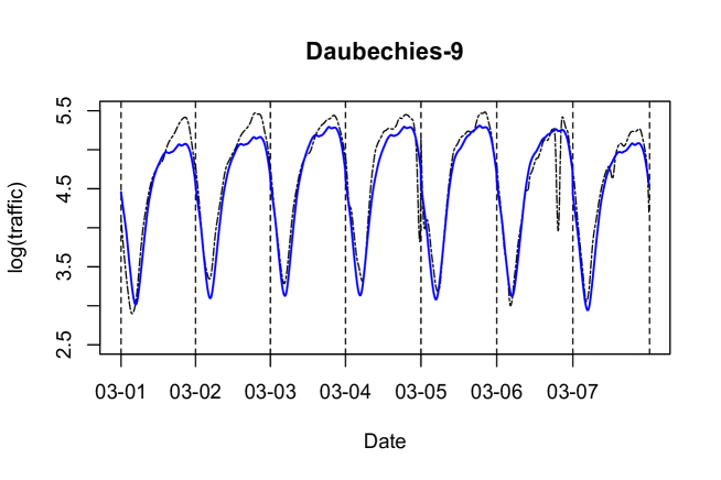
Figure 2: True functional data in black dashed curve and one-step ahead prediction based on sieve method with Daubechies-9 wavelets in blue solid curve for March 1st–7th.

References

- [1] A. Aue and J. Klepsch. Estimating functional time series by moving average model fitting. arXiv:1701.00770, 2017.
- [2] A. Aue, D. D. Norinho, and S. Hörmann. On the prediction of stationary functional time series. Journal of the American Statistical Association, 110(509):378–392, 2015.
- [3] U. Beyaztas and H. L. Shang. On function-on-function regression: partial least squares approach. Environmental and Ecological Statistics, 27:95–114, 2020.
- [4] W. W. Biao and Z. Zhou. Gaussian approximations for non-stationary multiple time series. Statistica Sinica, 21:1397–1413, 2011.
- [5] G. Biau and B. Patra. Sequential quantile prediction of time series. IEEE Transactions on Information Theory, 57:1664–1674, 2011.
- [6] D. Bosq. Linear Processes in Function Spaces. Springer-Verlag, 2000.
- [7] P. Brockwell and R. Davis. Time series: Theory and Methods (Second Edition)., volume Second Edition. Springer-Verlag, 1991.
- [8] T. T. Cai, W. Liu, and H. H. Zhou. Estimating sparse precision matrix: Optimal rates of convergence and adaptive estimation. The Annals of Statistics, 44(2):455–488, 2016.
- [9] X. Chen. Large sample sieve estimation of semi-nonparametric models. Handbook of Econometrics, 6:5549–5632, 2007.
- [10] X. Chen, M. Xu, and W. B. Wu. Covariance and precision matrix estimation for high-dimensional time series. The Annals of Statistics, 41(6):2994 – 3021, 2013.
- [11] Y. Chen, W. S. Chua, and T. Koch. Forecasting day-ahead high-resolution natural-gas demand and supply in Germany. Applied Energy, 228(15):1091–1110, 2018.
- [12] J.-M. Chiou, Y.-F. Yang, and Y.-T. Chen. Multivariate functional principal component analysis: A normalization approach. Statistica Sinica, 24(4):1571–1596, 2014.
- [13] S. Das and D. N. Politis. Predictive inference for locally stationary time series with an application to climate data. Journal of the American Statistical Association, 116(534):919–934, 2021.
- [14] H. Dette and W. Wu. Prediction in locally stationary time series. Journal of Business & Economic Statistics, 40(1):370–381, 2022.
- [15] X. Ding and Z. Zhou. Auto-regressive approximations to non-stationary time series, with inference and applications. arXiv:2112.00693v2, 2023.
- [16] F. Ferraty and P. Vieu. Functional nonparametric statistics: a double infinite dimensional framework. North-Holland, Amsterdam, 2003. In Recent Advances and Trends in Nonparametric Statistics (M. G. Akritas and D. N. Politis, eds.).
- [17] P. Fryzlewicz, S. V. Bellegem, and R. von Sachs. Forecasting non-stationary time series by wavelet process modelling. Annals of the Institute of Statistical Mathematics, 55:737–764, 2003.
- [18] Y. Fu, Z. Su, B. Xu, and Y. Zhou. Forecasting stock index futures intraday returns: Functional time series model. Journal of Advanced Computational Intelligence and Intelligent Informatics, 24(3):265–271, 2020.
- [19] Y. Gao and H. Shang. Multivariate functional time series forecasting: Application to age-specific mortality rates. Risks, 5(21):1–18, 2017.
- [20] L. Gyorfi and G. Ottucsak. Sequential prediction of unbounded stationary time series. IEEE Transactions on Information Theory, 53(5):1866–1872, 2007.
- [21] P. Hall and M. Hosseini-Nasab. On properties of functional principal components analysis. Journal of the Royal Statistical Society: Series B (Statistical Methodology), 68(1):109–126, 2006.
- [22] S. Hays, H. Shen, and J. Z. Huang. Functional dynamic factor models with application to yield curve forecasting. The Annals of Applied Statistics, 6(3):870–894, 2012.
- [23] L. Horváth, P. Kokoszka, and G. Rice. Testing stationarity of functional time series. Journal of Econometrics, 179(1):66–82, 2014.
- [24] J. Z. Huang. Projection estimation in multiple regression with application to functional ANOVA models. The Annals of Statistics, 26(1):242–272, 1998.
- [25] R. J. Hyndman and H. L. Shang. Forecasting functional time series (with discussion). Journal of the Korean Statistical Society, 38(3):199–221, 2009.
- [26] R. J. Hyndman and M. S. Ullah. Robust forecasting of mortality and fertility rates: a functional data approach. Computational Statistics & Data Analysis, 51(10):4942–4956, 2007.
- [27] J. Klepsch, C. Klüppelberg, and T. Wei. Prediction of functional ARMA processes with an application to traffic data. Econometric and Statistics, 1:128–149, 2017.
- [28] P. Kokoszka, H. Miao, and X. Zhang. Functional dynamic factor model for intraday price curves. Journal of Financial Econometrics, 13(2):456–477, 2015.
- [29] P. Kokoszka and M. Reimherr. Determining the order of the functional autoregressive model. Journal of Time Series Analysis, 34(1):116–129, 2013.
- [30] P. Kokoszka and M. Reimherr. Introduction to Functional Data Analysis. Chapman and Hall/CRC, 2017.
- [31] P. Kokoszka and X. Zhang. Functional prediction of intraday cumulative returns. Statistical Modelling, 12(4):377–398, 2012.
- [32] A. N. Kolmogorov. Interpolation and extrapolation of stationary random sequence. Izvestiya the Academy of Sciences of the USSR, Ser. Math., 5:3–14, 1941.
- [33] D. Kurisu. On the estimation of locally stationary functional time series. arXiv:2105.11873, 2023.
- [34] Y. Li and T. Hsing. On rates of convergence in functional linear regression. Journal of Multivariate Analysis, 98(9):1782–1804, 2007.
- [35] Y. Meyer. Ondelettes et oṕ erateurs. Actualités mathématiques. Hermann, Paris, 1990.
- [36] W. K. Newey. Convergence rates and asymptotic normality for series estimators. Journal of Econometrics, 79(1):147–168, 1997.
- [37] A. B. Nobel. On optimal sequential prediction for general processes. IEEE Transactions on Information Theory, 49(1):83–98, 2003.
- [38] C. Preda and G. Saporta. Pls regression on a stochastic process. Computational Statistics and Data Analysis, 48(1):149–158, 2005.
- [39] F. Roueff and A. Sánchez-Pérez. Prediction of weakly locally stationary processes by auto-regression. ALEA, Lat. Am. J. Probab. Math. Stat, 15:1215–1239, 2018.
- [40] D. Schafer. Strongly consistent online forecasting of centered Gaussian processes. IEEE Transactions on Information Theory, 48(3):791–799, 2002.
- [41] I. Shah and F. Lisi. Day-ahead electricity demand forecasting with nonparametric functional models. In 12th International Conference on the European Energy Market (EEM), 2015. pp 1–5.
- [42] H. L. Shang. A survey of functional principal component analysis. AStA Advances in Statistical Analysis, 98(1):121–142, 2014.
- [43] H. L. Shang. A robust functional time series forecasting method. Journal of Statistics Computation and Simulation, 89(5):795–814, 2019.
- [44] H. L. Shang and R. J. Hyndman. Nonparametric time series forecasting with dynamic updating. Mathematics and Computers in Simulation, 81(7):1310–1324, 2011.
- [45] L. N. Trefethen. Is Gauss quadrature better than Clenshaw–Curtis? SIAM review, 50(1):67–87, 2008.
- [46] A. van Delft and M. Eichler. Locally stationary functional time series. Electronic Journal of Statistics, 12(1):107–170, 2018.
- [47] J. Vilar, G. Aneiros, and P. Raña. Prediction intervals for electricity demand and price using functional data. International Journal of Electrical Power & Energy Systems, 96:457–472, 2018.
- [48] H. Wang and S. Xiang. On the convergence rates of Legendre approximation. Mathematics of Computation, 81(278):861–877, 2011.
- [49] N. Wiener. Extrapolation, interpolation and smoothing of stationary time series. New York, Wiley, 1949.
- [50] C. Y. and B. Li. An adaptive functional autoregressive forecast model to predict electricity price curves. Journal of Business & Economic Statistics, 35(3):371–388, 2017.
- [51] X. Zhang and G. Cheng. Gaussian approximation for high dimensional vector under physical dependence. Bernoulli, 24(4A):2640–2675, 2018.
- [52] Z. Zhou, Z. Xu, and W. B. Wu. Long-term prediction intervals of time series. IEEE Transcations on Information Theory, 56(3):1436–1446, 2010.