Successive Linear Approximation VBI for Joint Sparse Signal Recovery and Dynamic Grid Parameters Estimation

Abstract

For many practical applications in wireless communications, we need to recover a structured sparse signal from a linear observation model with dynamic grid parameters in the sensing matrix. Conventional expectation maximization (EM)-based compressed sensing (CS) methods, such as turbo compressed sensing (Turbo-CS) and turbo variational Bayesian inference (Turbo-VBI), have double-loop iterations, where the inner loop (E-step) obtains a Bayesian estimation of sparse signals and the outer loop (M-step) obtains a point estimation of dynamic grid parameters. This leads to a slow convergence rate. Furthermore, each iteration of the E-step involves a complicated matrix inverse in general. To overcome these drawbacks, we first propose a successive linear approximation VBI (SLA-VBI) algorithm that can provide Bayesian estimation of both sparse signals and dynamic grid parameters. Besides, we simplify the matrix inverse operation based on the majorization-minimization (MM) algorithmic framework. In addition, we extend our proposed algorithm from an independent sparse prior to more complicated structured sparse priors, which can exploit structured sparsity in specific applications to further enhance the performance. Finally, we apply our proposed algorithm to solve two practical application problems in wireless communications and verify that the proposed algorithm can achieve faster convergence, lower complexity, and better performance compared to the state-of-the-art EM-based methods.

I Introduction

Compressed sensing (CS) has been widely used in many applications, such as channel estimation [1, 2, 3], data detection [4, 5], target localization [6, 7], etc. For a standard compressed sensing problem, a sparse signal $\boldsymbol{x}\in\mathbb{C}^{N\times 1}$ is to be recovered from measurements $\boldsymbol{y}\in\mathbb{C}^{M\times 1}$ ($M<N$) under a linear observation model,

$$\boldsymbol{\boldsymbol{y}}=\mathbf{F}\boldsymbol{x}+\boldsymbol{w},$$ (1)

where the sensing matrix $\mathbf{F}\in\mathbb{C}^{M\times N}$ is fixed and perfectly known, and the noise vector $\boldsymbol{w}\in\mathbb{C}^{M\times 1}$ follows a complex Gaussian distribution with noise variance $\gamma^{-1}$. However, in many practical scenarios, some dynamic grid parameters may exist in the sensing matrix. For instance, in massive multiple-input multiple-output (MIMO) systems, the angular-domain dynamic gird parameters are usually introduced for high-performance channel estimation [8]. In this case, the observation model in $(\ref{eq:strandard model})$ can be rewritten into

$$\boldsymbol{\boldsymbol{y}}=\mathbf{F}\left(\boldsymbol{\theta}\right)\boldsymbol{x}+\boldsymbol{w},$$ (2)

where $\boldsymbol{\theta}$ denotes the dynamic grid parameters. Our primary goal is to recover the sparse signal $\boldsymbol{x}$ and estimate the dynamic grid parameters $\boldsymbol{\theta}$ simultaneously given observations $\boldsymbol{y}$. There are three common methods in the literature.

On-grid based CS methods: The main idea of the on-grid based method is to select a fixed sampling grid and use discrete grid points to approximate the true parameters $\boldsymbol{\theta}$. The conventional CS method is a good choice under the on-grid based model, such as orthogonal matching pursuit (OMP) [9], $\ell_{1}$-norm optimization [10, 11], and sparse Bayesian learning/inference [12, 13, 14]. In practice, the true parameters $\boldsymbol{\theta}$ usually do not lie exactly on the fixed grid points. And thus the estimation accuracy of $\boldsymbol{\theta}$ is limited by the grid resolution. To reduce the mismatch between the true parameter and its nearest grid point, a dense sampling grid is needed. However, a dense sampling grid leads to a highly correlated sensing matrix and a poor estimate of the sparse signal.

Off-grid sparse Bayesian inference (OGSBI): It is very challenging to directly estimate $\boldsymbol{\theta}$ since the mapping $\boldsymbol{\theta}\rightarrow\mathbf{F}\left(\boldsymbol{\theta}\right)$ is nonlinear. To address this difficulty, the authors in [15, 16] approximated the basis vectors of the sensing matrix using linearization. The proposed OGSBI algorithm achieved a better performance than the on-grid based CS methods. However, the error caused by linear approximation is not completely eliminated due to the absence of high-order items of Taylor expansion. In [17], the authors improved the OGSBI algorithm and proposed a new weighted OGSBI algorithm based on second-order Taylor expansion approximation. Another main drawback of the OGSBI is that the Laplace prior model used in [15, 16, 17] can only exploit an i.i.d. sparse structure.

Expectation maximization (EM)-based methods: The EM-based methods contain two major steps, where the E-step computes a Bayesian estimation of $\boldsymbol{x}$ and the M-step gives a point estimation of $\boldsymbol{\theta}$. To describe different type of sparse structures, some recent literature usually adopted the turbo approach as the E-step. In [18], the authors proposed a novel turbo approximate message passing (Turbo-AMP) for loopy belief propagation. Inspired by this work, the E-step in [19, 20, 21] was a turbo compressed sensing (Turbo-CS) framework, by combining the linear minimum mean square error (LMMSE) estimator with message passing. In [22, 23], the authors proposed a turbo variational Bayesian inference (Turbo-VBI) algorithm by combining the VBI estimator with message passing. The EM-based methods can exploit more complicated sparse structures and achieve better performance than the first two methods. However, the computational complexity of these methods are often higher. In the first place, the Bayesian estimator in the E-step usually involves a matrix inverse in each iteration. Although it is possible to avoid matrix inverse for a few special choices of sensing matrix (such as Turbo-AMP for an i.i.d. sensing matrix and Turbo-CS for a partially orthogonal sensing matrix), the sensing matrices in many important practical applications do not belong to these special cases, especially under the consideration of dynamic grid parameters. Secondly, the EM-based methods involve double-loop iterations, i.e., the inner iteration involved in the E-step (Bayesian estimator) and the outer iteration between the E-step and M-step.

In this paper, we propose an inverse-free successive linear approximation VBI algorithm to overcome the drawbacks of the existing methods. The proposed algorithm can output the Bayesian estimation of both sparse signals and dynamic grid parameters, and it can achieve lower complexity, faster convergence, and better performance compared to the state-of-the-art EM-based Turbo-CS and Turbo-VBI algorithms. The main contributions are summarized below.

• Successive linear approximation VBI (SLA-VBI): We aim at computing the approximate posterior distribution of both sparse signals and dynamic grid parameters based on the VBI iterations. Using the successive linear approximation approach, the Bayesian inference can be performed in closed form. In contrast to the double-loop EM-based methods, the proposed SLA-VBI reduces the number of iterations significantly while speeding up convergence.

• Inverse-free algorithm design: Conventional sparse Bayesian inference algorithms usually involve the matrix inverse operation during iterations. To reduce the computational overhead, we adopt the majorization-minimization (MM) [24] framework to avoid the matrix inverse and propose a low-complexity inverse-free successive linear approximation VBI (IFSLA-VBI) algorithm. The proposed IFSLA-VBI can achieve a better trade-off between performance and complexity by controlling the number of iterations used to approximate the matrix inverse according to the structure of the sensing matrix.

• Extension to structured sparse priors for practical applications: In practical applications, the sparse signal $\boldsymbol{x}$ usually has structured sparsity. To exploit the specific sparse structures, we extend our proposed algorithm from an independent sparse prior to more complicated structured sparse priors and apply it to solve important practical problems in wireless communications.

The rest of the paper is organized as follows. In Section II, we introduce a three-layer sparse prior model and present the system model of two practical applications. In Section III, we introduce the proposed SLA-VBI and IFSLA-VBI algorithms. In Section IV, we elaborate on how to extend the proposed algorithm to structured sparse priors. Simulation results and conclusions are shown in Section V and VI, respectively.

Notation: Lowercase boldface letters denote vectors and uppercase boldface letters denote matrices. $\left(\cdot\right)^{-1}$, $\left(\cdot\right)^{T}$, $\left(\cdot\right)^{H}$, $\left\|\cdot\right\|$, $\left\langle\cdot\right\rangle$, and $\textrm{diag}\left(\cdot\right)$ are used to represent the inverse, transpose, conjugate transpose, $\ell_{2}\textrm{-norm}$, expectation, and diagonalization operations, respectively. Let $\mathfrak{Re}\left\{\cdot\right\}$ denote the real part of the complex argument. For a set $\mathcal{N}$, we use $\left|\mathcal{N}\right|$ to denote its cardinality. Let $\boldsymbol{x}\triangleq\left[x_{n}\right]_{n\in\mathcal{N}}\in\mathbb{C}^{\left|\mathcal{N}\right|\times 1}$ represent a vector composed of elements indexed by $\mathcal{N}$. $\mathcal{CN}\left(\boldsymbol{x};\boldsymbol{\mu},\mathbf{\Sigma}\right)$ represents a complex Gaussian distribution with mean $\boldsymbol{\mu}$ and covariance matrix $\mathbf{\Sigma}$. $\textrm{Ga}\left(x;a,b\right)$ represents a Gamma distribution with shape parameter $a$ and rate parameter $b$.

II System Model

II-A Three-layer Sparse Prior Model

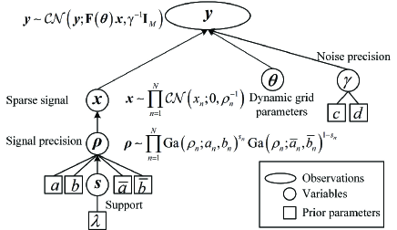
Figure 1: Illustration of the three-layer hierarchical sparse prior model.

We introduce a three-layer sparse prior model [22, 23] that can describe various sparse structures, as illustrated in Fig. 1. Specifically, we use a binary vector $\boldsymbol{s}\triangleq\left[s_{1},\ldots,s_{N}\right]^{T}$ to represent the support of $\boldsymbol{x}$, where $s_{n}=1$ indicates $x_{n}$ is non-zero and $s_{n}=0$ indicates the opposite. Let $\boldsymbol{\rho}\triangleq\left[\rho_{1},\ldots,\rho_{N}\right]^{T}$ denote the precision vector of $\boldsymbol{x}$, where $1/\rho_{n}$ is the variance of $x_{n}$. The joint distribution of $\boldsymbol{x}$, $\boldsymbol{\rho}$, and $\boldsymbol{s}$ can be expressed as

$$p\left(\boldsymbol{x},\boldsymbol{\rho},\boldsymbol{s}\right)=\underbrace{p\left(\boldsymbol{s}\right)}_{\textrm{Support}}\underbrace{p\left(\boldsymbol{\rho}\mid\boldsymbol{s}\right)}_{\textrm{Precision}}\underbrace{p\left(\boldsymbol{x}\mid\boldsymbol{\rho}\right)}_{\textrm{Sparse\ signal}}.$$ (3)

A complex Gaussian distribution is assumed as the prior for $\boldsymbol{x}$. Moreover, conditioned on $\boldsymbol{\rho}$, the elements of $\boldsymbol{x}$ are independent, i.e.,

$$p\left(\boldsymbol{x}\mid\boldsymbol{\rho}\right)=\prod_{n=1}^{N}p\left(x_{n}\mid\rho_{n}\right)=\prod_{n=1}^{N}\mathcal{CN}\left(x_{n};0,\rho_{n}^{-1}\right).$$ (4)

The precision vector $\boldsymbol{\rho}$ can be expressed with the Bernoulli-Gamma distribution

$$p\left(\boldsymbol{\rho}\mid\boldsymbol{s}\right)= \prod_{n=1}^{N}\textrm{Ga}\left(\rho_{n};a_{n},b_{n}\right)^{s_{n}}\textrm{Ga}\left(\rho_{n};\overline{a}_{n},\overline{b}_{n}\right)^{1-s_{n}},$$ (5)

where $a_{n}$, $b_{n}$ and $\overline{a}_{n}$, $\overline{b}_{n}$ are prior parameters of $\rho_{n}$ conditioned on $s_{n}=1$ and $s_{n}=0$, respectively. To indicate $x_{n}$ is zero or non-zero more effectively, $a_{n}$ and $b_{n}$ are chosen to satisfy $\frac{a_{n}}{b_{n}}=\mathbb{E}\left(\rho_{n}\mid s_{n}=1\right)=\Theta\left(1\right)$, while $\overline{a}_{n}$ and $\overline{b}_{n}$ are chosen to satisfy $\frac{a_{n}}{b_{n}}=\mathbb{E}\left(\rho_{n}\mid s_{n}=0\right)\gg 1$ [22, 23].

The prior for the support vector depends on the specific sparse structure. For example, for an independent sparse structure, a Bernoulli distribution is usually used as the prior,

$$p\left(\boldsymbol{s}\right)=\prod_{n=1}^{N}\left(\lambda_{n}\right)^{s_{n}}\left(1-\lambda_{n}\right)^{1-s_{n}},$$ (6)

where $\lambda_{n}$ gives the probability of $p\left(s_{n}=1\right)$. For more complicated sparse structures, we use other sparse priors to capture the specific structured sparsity. And our proposed algorithm can be easily extended to these cases via the turbo approach. We will elaborate on the extended algorithm in Section IV.

Meanwhile, we employ a gamma distribution with parameters $c$ and $d$ to model the noise precision, i.e.,

$$p\left(\gamma\right)=\textrm{Ga}\left(\gamma;c,d\right).$$ (7)

II-B Problem Statement

Recall the linear observation model with dynamic grid parameters in the sensing matrix

$$\boldsymbol{\boldsymbol{y}}=\mathbf{F}\left(\boldsymbol{\theta}\right)\boldsymbol{x}+\boldsymbol{w}.$$ (8)

According to the physical meaning, we partition $\boldsymbol{\theta}$ into $B$ blocks $\boldsymbol{\theta}\triangleq\bigl{\{}\boldsymbol{\theta}^{1},\ldots,\boldsymbol{\theta}^{B}\bigr{\}}$ , such that each block $\boldsymbol{\theta}^{j}\triangleq\bigl{[}\theta_{1}^{j},\ldots,\theta_{N}^{j}\bigr{]}^{T}\in\mathbb{C}^{N\times 1},j\in\left\{1,\ldots,B\right\}$ denotes a type of dynamic grid parameters. For example, we partition dynamic grid parameters into distance parameters $\boldsymbol{\iota}$ and angle parameters $\boldsymbol{\vartheta}$ in subsection II-D. Let $\mathbf{F}\left(\boldsymbol{\theta}\right)\triangleq\left[\boldsymbol{\varPhi}\left(\boldsymbol{\theta}_{1}\right),\ldots,\boldsymbol{\varPhi}\left(\boldsymbol{\theta}_{N}\right)\right]$, where $\boldsymbol{\theta}_{n}\triangleq\bigl{[}\theta_{n}^{1},\ldots,\theta_{n}^{B}\bigr{]}^{T}$ denotes parameters of the $n\textrm{-th}$ basis vector $\boldsymbol{\varPhi}\left(\boldsymbol{\theta}_{n}\right)$ for $n=1,\ldots,N$. Our primary goal is to compute the Bayesian estimation of the sparse signal $\boldsymbol{x}$, the support vector $\boldsymbol{s}$, and the dynamic grid parameters $\boldsymbol{\theta}$ given the observations $\boldsymbol{y}$. Such a joint sparse signal recovery and dynamic grid estimation problem includes many important application problems as special cases. In the following two subsections, we shall present two application examples.

II-C Massive MIMO Channel Estimation with Limited Pilots

Consider a narrow-band massive MIMO system with a base station (BS) serving a single-antenna user, as shown in Fig. 2. The BS is equipped with a uniform linear array (ULA) of $N\gg 1$ antennas. To estimate the downlink channel vector $\boldsymbol{h}\in\mathbb{C}^{N\times 1}$, the BS transmits pilot sequences $\boldsymbol{u}_{t}\in\mathbb{C}^{N\times 1},t=1,\ldots,M$ ($M<N$) to the user. The received signal $\boldsymbol{y}\in\mathbb{C}^{M\times 1}$ can be expressed as

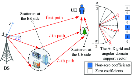
Figure 2: Illustration of the massive MIMO downlink channel and its non-zero coefficients.

$$\boldsymbol{y}=\mathbf{U}\boldsymbol{h}+\boldsymbol{w},$$ (9)

where $\mathbf{U}\triangleq\left[\boldsymbol{u}_{1},\ldots,\boldsymbol{u}_{M}\right]^{T}\in\mathbb{C}^{M\times N}$ denotes the pilot matrix and $\boldsymbol{w}\sim\mathcal{CN}\left(\boldsymbol{w};0,\gamma^{-1}\mathbf{I}_{M}\right)$ is the Gaussian noise. Assume there are $L$ paths for the communication channel, the channel vector $\boldsymbol{h}$ can be modeled as

$$\boldsymbol{h}=\sum_{l=1}^{L}x_{l}\boldsymbol{a}\left(\theta_{l}\right),$$ (10)

where $x_{l}$ and $\theta_{l}$ denote the complex channel gain and angle-of-departure (AoD) of the $l\textrm{-th}$ path, respectively. The steer vector at the BS is given by

$$\boldsymbol{a}\bigl{(}\theta\bigr{)}\triangleq\frac{1}{\sqrt{N}}\left[1,e^{j\pi\sin\theta},\ldots,e^{j\left(N-1\right)\pi\sin\theta}\right]^{T}.$$ (11)

To obtain a sparse representation of the channel vector, we adopt the grid-based solution. Specifically, we define a fixed grid $\left\{\overline{\vartheta}_{1},\ldots,\overline{\vartheta}_{\widetilde{N}}\right\}$ of $\widetilde{N}$ AoD points such that $\left\{\sin\overline{\vartheta}_{n}\right\}_{n=1}^{{}_{\widetilde{N}}}$ are uniformly distributed in the range $\left[-1,1\right]$.

However, the true AoDs usually do not lie exactly on $\widetilde{N}$ discrete AoD grid points. In this case, the gap between the true AoD and its nearest grid point will lead to energy leakage. To mitigate the effect of energy leakage, we introduce a dynamic AoD grid $\boldsymbol{\vartheta}=\left[\vartheta_{1},\ldots,\vartheta{}_{\widetilde{N}}\right]^{T}$ instead of only using a fixed sampling grid . In the algorithm design, the grid parameters $\boldsymbol{\vartheta}$ will be updated via Bayesian inference for more accurate channel estimation.

Based on the definition of the dynamic AoD grid, we can obtain a sparse basis $\mathbf{A}\left(\boldsymbol{\vartheta}\right)\triangleq\left[\boldsymbol{a}\left(\vartheta_{1}\right),\ldots,\boldsymbol{a}\left(\vartheta{}_{\widetilde{N}}\right)\right]\in\mathbb{C}^{N\times\widetilde{N}}$. The sparse representation of the channel vector in (10) is given by

$$\boldsymbol{h}=\mathbf{A}\left(\boldsymbol{\vartheta}\right)\boldsymbol{x},$$ (12)

where $\boldsymbol{x}\in\mathbb{C}^{\widetilde{N}\times 1}$ is the angular-domain sparse channel vector. $\boldsymbol{x}$ has only $L$ non-zero elements corresponding to the AoDs of $L\ll\widetilde{N}$ paths. Let $\boldsymbol{s}\triangleq\bigl{[}s_{1},\ldots,s_{{}_{\widetilde{N}}}\bigr{]}^{T}$ denote the support vector of $\boldsymbol{x}$, where $s_{n}=1$ indicates there is a channel path with AoD $\vartheta_{n}$, while $s_{n}=0$ indicates the opposite.

Then the received signal in (9) can be rewritten into

$$\boldsymbol{y}=\mathbf{F}\left(\boldsymbol{\vartheta}\right)\boldsymbol{x}+\boldsymbol{w},$$ (13)

where $\mathbf{F}\left(\boldsymbol{\vartheta}\right)\triangleq\mathbf{U}\mathbf{A}\left(\boldsymbol{\vartheta}\right)$.

For such a linear observation model with dynamic grid parameters in the sensing matrix, our goal is to recover the angular-domain sparse channel vector $\boldsymbol{x}$, the support vector $\boldsymbol{s}$, and the AoD grid parameters $\boldsymbol{\vartheta}$ from the received signal $\boldsymbol{y}$.

II-D 6G-based Target Detection and Localization

Consider a broadband MIMO Orthogonal Frequency Division Multiplexing (OFDM) system with a BS equipped with $N$ antennas and $N_{\textrm{RF}}<N$ radio frequency (RF) chains, as illustrated in Fig. 3. In future 6G wireless systems, the MIMO-OFDM signal will also be exploited to provide target sensing functionality [25, 26]. For simplicity, we consider that all targets are on a two-dimensional (2-D) plane. Note that our results can be easily extended to a 3-D environment. We assume there are $K$ targets in the area, and the polar coordinates of the $k\textrm{-th}$ target is represented as $\boldsymbol{p}_{k}\triangleq\left(r_{k},\theta_{k}\right)$, where $r_{k}$ is its distance from the BS and $\theta_{k}$ is its angle.

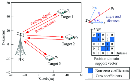
Figure 3: A target detection and localization model in 6G MIMO-OFDM systems and the non-zero coefficients of the virtual position-domain channel.

To sense the presence of the targets and estimate the associated parameters, on the $n\textrm{-th}$ subcarrier for $n\in\mathcal{N}_{b}$, the BS sends a probing signal $\boldsymbol{u}_{n}\in\mathbb{C}^{N\times 1}$. Then the reflected echo signal $\boldsymbol{\boldsymbol{y}}_{n}\in\mathbb{C}^{N_{\textrm{RF}}\times 1}$ can be expressed as

$$\boldsymbol{\boldsymbol{y}}_{n}=\mathbf{W}_{\textrm{RF}}\mathbf{H}_{n}\boldsymbol{u}_{n}+\boldsymbol{w}_{n},\forall n\in\mathcal{N}_{b},$$ (14)

where $\mathbf{W}_{\textrm{RF}}\in\mathbb{C}^{N_{\textrm{RF}}\times N}$ is the RF combining matrix, $\boldsymbol{w}_{n}\sim\mathcal{CN}\left(\boldsymbol{w}_{n};0,\gamma^{-1}\mathbf{I}_{N_{\textrm{RF}}}\right)$ is the noise vector, and the channel matrix $\mathbf{H}_{n}\in\mathbb{C}^{N\times N}$ is modeled as

$$\mathbf{H}_{n}=\sum_{k=1}^{K}x_{k}e^{-j2\pi\left(n-1\right)f_{0}\tau_{k}}\boldsymbol{a}\left(\theta_{k}\right)\boldsymbol{a}^{T}\left(\theta_{k}\right),$$ (15)

where $x_{k}$ is the complex reflection coefficient of the $k\textrm{-th}$ target and $f_{0}$ is the subcarrier interval. The propagation delay is denoted by $\tau_{k}=2r_{k}/c$, where $c$ is the speed of light.

Similar to subsection II-C, we introduce a dynamic position grid $\left\{\boldsymbol{\iota},\boldsymbol{\vartheta}\right\}\triangleq\left\{\left(\iota_{1},\vartheta_{1}\right),\ldots,\left(\iota_{Q},\vartheta_{Q}\right)\right\}$ of $Q$ position grid points for high-accuracy target localization, where $\boldsymbol{\iota}$ and $\boldsymbol{\vartheta}$ denote distance and angle parameters, respectively.

With the definition of the dynamic position grid, we define a sparse basis as

$$\mathbf{B}_{n}\left(\boldsymbol{\iota},\boldsymbol{\vartheta}\right)\triangleq\left[\boldsymbol{b}_{n,1},\ldots,\boldsymbol{b}_{n,Q}\right]\in\mathbb{C}^{N\times Q},\forall n\in\mathcal{N}_{b},$$

where the basis vector is given by

$$\boldsymbol{b}_{n,q}\triangleq e^{-j2\pi\left(n-1\right)f_{0}\frac{2\iota_{q}}{c}}\boldsymbol{a}\left(\vartheta_{q}\right)\boldsymbol{a}^{T}\left(\vartheta_{q}\right)\boldsymbol{u}_{n},\forall n\in\mathcal{N}_{b},\forall q.$$

Then the echo signal in (14) can be rewritten into

$$\boldsymbol{\boldsymbol{y}}_{n}=\mathbf{W}_{\textrm{RF}}\mathbf{B}_{n}\left(\boldsymbol{\iota},\boldsymbol{\vartheta}\right)\boldsymbol{x}+\boldsymbol{w}_{n},\forall n\in\mathcal{N}_{b},$$ (16)

where $\boldsymbol{x}\triangleq\left[x_{1},\ldots,x_{Q}\right]^{T}\in\mathbb{C}^{Q\times 1}$ is called the position-domain sparse channel vector. We use $\boldsymbol{s}\triangleq\left[s_{1},\ldots,s_{Q}\right]^{T}$ to represent the support vector of $\boldsymbol{x}$, where $s_{q}=1$ indicates there is a target lying in the $q\textrm{-th}$ position grid with angle $\vartheta_{q}$ and distance $\iota_{q}$, while $s_{q}=0$ indicates the opposite.

Using (16), the received echo signal on all available subcarriers can be obtained as

$$\boldsymbol{\boldsymbol{y}}=\mathbf{F}\left(\boldsymbol{\iota},\boldsymbol{\vartheta}\right)\boldsymbol{x}+\boldsymbol{w},$$ (17)

where $\boldsymbol{\boldsymbol{y}}\triangleq\left[\boldsymbol{y}_{n}\right]_{n\in\mathcal{N}_{b}}$, $\mathbf{F}\left(\boldsymbol{\iota},\boldsymbol{\vartheta}\right)\triangleq\left[\mathbf{W}_{\textrm{RF}}\mathbf{B}_{n}\bigl{(}\boldsymbol{\iota},\boldsymbol{\vartheta}\bigr{)}\right]_{{}_{n\in\mathcal{N}_{b}}}$, and $\boldsymbol{w}\triangleq\left[\boldsymbol{w}_{n}\right]_{n\in\mathcal{N}_{b}}$.

For a target detection and localization problem, we aim at estimating the support vector $\boldsymbol{s}$ and the position grid parameters $\left\{\boldsymbol{\iota},\boldsymbol{\vartheta}\right\}$ from the received echo signal $\boldsymbol{y}$.

III Successive Linear Approximation VBI

III-A Mean Field VBI

We first give an overview of the mean field variational Bayesian inference. Let $\boldsymbol{v}\triangleq\left\{\boldsymbol{x},\boldsymbol{\rho},\boldsymbol{s},\gamma,\boldsymbol{\theta}\right\}$ denote the collection of hidden variables in (8). For convenience, we use $\boldsymbol{v}^{l}$ to denote an individual variable in $\boldsymbol{v}$ and let $\mathcal{H}\triangleq\left\{l\mid\forall\boldsymbol{v}^{l}\in\boldsymbol{v}\right\}$. We aim at calculating the posterior distribution of hidden variables, i.e., $p\left(\boldsymbol{v}\mid\boldsymbol{y}\right)$. However, it is usually intractable to find the posterior directly since the considered problem involves integrals of many high-dimensional variables. Based on the mean field VBI method, the posterior distribution is approximated by the variational distribution $q\left(\boldsymbol{v}\right)$ that minimizes the Kullback-Leibler (KL) divergence between $q\left(\boldsymbol{v}\right)$ and $p\left(\boldsymbol{v}\mid\boldsymbol{y}\right)$ under a factorized form constraint as

$$\min_{q\left(\boldsymbol{v}\right)} \mathrm{KL}\left(q\bigparallel p\right) \triangleq\int q\left(\boldsymbol{v}\right)\ln\frac{q\left(\boldsymbol{v}\right)}{p\left(\boldsymbol{v}\mid\boldsymbol{\boldsymbol{y}}\right)}\mathrm{d}\boldsymbol{v},$$ (18)

$$s.t. q\left(\boldsymbol{v}\right) =\prod_{l\in\mathcal{H}}q\left(\boldsymbol{v}^{l}\right),$$

where the constraint $q\left(\boldsymbol{v}\right)=\prod_{l\in\mathcal{H}}q\left(\boldsymbol{v}^{l}\right)$ is the mean field assumption [27]. Note that the dynamic grid $\boldsymbol{\theta}$ is also viewed as a hidden variable in algorithm design, which is quite different from the conventional VBI in [22, 23]. And thus, our proposed algorithm can provide the Bayesian estimation of $\boldsymbol{\theta}$ additionally.

Although the problem (18) is known to be non-convex, it is convex w.r.t a single variational distribution $q\left(\boldsymbol{v}^{l}\right)$ after fixing other variational distributions $q\left(\boldsymbol{v}^{k}\right),\forall k\neq l$ [28]. And it has been proved in [28] that a stationary solution could be found via optimizing each variational distribution in an alternating fashion. Specifically, for given $q\left(\boldsymbol{v}^{k}\right),\forall k\neq l$, the optimal $q\left(\boldsymbol{v}^{l}\right)$ that minimizes the KL-divergence is given by [28]

$$q\bigl{(}\boldsymbol{v}^{l}\bigr{)}=\frac{\exp\left(\left\langle\ln p\left(\boldsymbol{v},\boldsymbol{y}\right)\right\rangle_{\Pi_{k\neq l}q\left(\boldsymbol{v}^{k}\right)}\right)}{\int\exp\left(\left\langle\ln p\left(\boldsymbol{v},\boldsymbol{y}\right)\right\rangle_{\Pi_{k\neq l}q\left(\boldsymbol{v}^{k}\right)}\right)\textrm{d}\boldsymbol{v}^{l}},$$ (19)

where $\left\langle\cdot\right\rangle_{\Pi_{k\neq l}q\left(\boldsymbol{v}^{k}\right)}$ is an expectation operation w.r.t. $q\left(\boldsymbol{v}^{k}\right)$ for $k\neq l$. The joint distribution $p\left(\boldsymbol{v},\boldsymbol{y}\right)$ is given by

$$p\left(\boldsymbol{v},\boldsymbol{y}\right) =p\left(\boldsymbol{y}\mid\boldsymbol{x},\boldsymbol{\theta},\gamma\right)p\left(\boldsymbol{x},\boldsymbol{\rho},\boldsymbol{s}\right)p\left(\gamma\right)p\left(\boldsymbol{\theta}\right),$$ (20)

where $p\left(\boldsymbol{y}\mid\boldsymbol{x},\boldsymbol{\theta},\gamma\right)=\mathcal{CN}\left(\boldsymbol{y};\mathbf{F}\left(\boldsymbol{\theta}\right)\boldsymbol{x},\gamma^{-1}\mathbf{I}_{M}\right)$ is the likelihood function, $p\left(\boldsymbol{x},\boldsymbol{\rho},\boldsymbol{s}\right)$ and $p\left(\gamma\right)$ are the priors given in (3) and (7), respectively, and $p\left(\boldsymbol{\theta}\right)$ is the prior for the dynamic grid $\boldsymbol{\theta}$.

By substituting the joint distribution (20) into (19), each optimal variational distribution $q\bigl{(}\boldsymbol{v}^{l}\bigr{)}$ can be derived. In the following, we shall provide the details of the derivation for each variational distribution.

III-A1 Update of $q\left(\boldsymbol{x}\right)$

Using (19) and ignoring the terms that are not related to $\boldsymbol{x}$, the posterior distribution $q\left(\boldsymbol{x}\right)$ can be derived as

$$\ln q\left(\boldsymbol{x}\right)\propto \left\langle\ln p\left(\boldsymbol{v},\boldsymbol{y}\right)\right\rangle_{q\left(\boldsymbol{\rho}\right)q\left(\boldsymbol{s}\right)q\left(\gamma\right)q\left(\boldsymbol{\theta}\right)}$$

$$\propto \left\langle\ln p\left(\boldsymbol{y}\mid\boldsymbol{x},\boldsymbol{\theta},\gamma\right)\right\rangle_{q\left(\gamma\right)q\left(\boldsymbol{\theta}\right)}+\left\langle\ln p\left(\boldsymbol{x}\mid\boldsymbol{\rho}\right)\right\rangle_{q\left(\boldsymbol{\rho}\right)}$$

$$\propto -\bigl{\langle}\gamma\bigr{\rangle}\left\langle\left\|\boldsymbol{y}-\mathbf{F}\left(\boldsymbol{\theta}\right)\boldsymbol{x}\right\|^{2}\right\rangle_{q\left(\boldsymbol{\theta}\right)}-\boldsymbol{x}^{H}\textrm{diag}\left(\left\langle\boldsymbol{\rho}\right\rangle\right)\boldsymbol{x}$$

$$\propto -\boldsymbol{x}^{H}\left(\left\langle\gamma\right\rangle\left\langle\mathbf{F}\left(\boldsymbol{\theta}\right)^{H}\mathbf{F}\left(\boldsymbol{\theta}\right)\right\rangle_{q\left(\boldsymbol{\theta}\right)}+\textrm{diag}\left(\left\langle\boldsymbol{\rho}\right\rangle\right)\right)\boldsymbol{x}$$

$$+2\mathfrak{Re}\left\{\boldsymbol{x}^{H}\left\langle\gamma\right\rangle\left\langle\mathbf{F}\left(\boldsymbol{\theta}\right)^{H}\right\rangle_{q\left(\boldsymbol{\theta}\right)}\boldsymbol{y}\right\}$$

$$\propto -\boldsymbol{x}^{H}\boldsymbol{\Sigma}_{x}^{-1}\boldsymbol{x}+2\mathfrak{Re}\left\{\boldsymbol{x}^{H}\boldsymbol{\Sigma}_{x}^{-1}\boldsymbol{\mu}_{x}\right\}.$$ (21)

Clearly, this is the exponent of a complex Gaussian distribution with mean $\boldsymbol{\mu}_{x}$ and covariance matrix $\boldsymbol{\Sigma}_{x}$ given by

$$\boldsymbol{\mu}_{x} =\boldsymbol{\Sigma}_{x}\left\langle\gamma\right\rangle\left\langle\mathbf{F}\left(\boldsymbol{\theta}\right)^{H}\right\rangle_{q\left(\boldsymbol{\theta}\right)}\boldsymbol{y},$$ (22)

$$\boldsymbol{\Sigma}_{x} =\left(\left\langle\gamma\right\rangle\left\langle\mathbf{F}\left(\boldsymbol{\theta}\right)^{H}\mathbf{F}\left(\boldsymbol{\theta}\right)\right\rangle_{q\left(\boldsymbol{\theta}\right)}+\textrm{diag}\left(\left\langle\boldsymbol{\rho}\right\rangle\right)\right)^{-1}.$$

III-A2 Update of $q\left(\boldsymbol{\rho}\right)$

The posterior distribution $q\left(\boldsymbol{\rho}\right)$ can be computed by

$$\ln q\left(\boldsymbol{\rho}\right)\propto \left\langle\ln p\left(\boldsymbol{v},\boldsymbol{y}\right)\right\rangle_{q\left(\boldsymbol{x}\right)q\left(\boldsymbol{s}\right)q\left(\gamma\right)q\left(\boldsymbol{\theta}\right)}$$

$$\propto \left\langle\ln p\left(\boldsymbol{x}\mid\boldsymbol{\rho}\right)\right\rangle_{q\left(\boldsymbol{x}\right)}+\left\langle\ln p\left(\boldsymbol{\rho}\mid\boldsymbol{s}\right)\right\rangle_{q\left(\boldsymbol{s}\right)}$$

$$\propto \sum_{n=1}^{N}\ln\rho_{n}-\sum_{n=1}^{N}\rho_{n}\left\langle x_{n}^{2}\right\rangle$$

$$+\sum_{n=1}^{N}\left\langle s_{n}\right\rangle\left[\left(a_{n}-1\right)\ln\rho_{n}-b_{n}\rho_{n}\right]$$

$$+\sum_{n=1}^{N}\left\langle 1-s_{n}\right\rangle\left[\left(\overline{a}_{n}-1\right)\ln\rho_{n}-\overline{b}_{n}\rho_{n}\right]$$

$$\propto \sum_{n=1}^{N}\left[\left\langle s_{n}\right\rangle a_{n}+\left\langle 1-s_{n}\right\rangle\overline{a}_{n}\right]\ln\rho_{n}$$

$$-\sum_{n=1}^{N}\left[\left\langle s_{n}\right\rangle b_{n}+\left\langle 1-s_{n}\right\rangle\overline{b}_{n}+\left\langle x_{n}^{2}\right\rangle\right]\rho_{n}$$

$$\propto \sum_{n=1}^{N}\left(\widetilde{a}_{n}-1\right)\ln\rho_{n}-\sum_{n=1}^{N}\widetilde{b}_{n}\rho_{n}.$$ (23)

And thus, $\boldsymbol{\rho}$ has a form of product of Gamma distributions

$$q\left(\boldsymbol{\rho}\right)=\prod_{n=1}^{N}\textrm{Ga}\left(\rho_{n};\widetilde{a}_{n},\widetilde{b}_{n}\right),$$ (24)

where the parameters $\widetilde{a}_{n}$ and $\widetilde{b}_{n}$ are respectively given by

$$\widetilde{a}_{n} =\left\langle s_{n}\right\rangle a_{n}+\left\langle 1-s_{n}\right\rangle\overline{a}_{n}+1,$$ (25)

$$\widetilde{b}_{n} =\left\langle s_{n}\right\rangle b_{n}+\left\langle 1-s_{n}\right\rangle\overline{b}_{n}+\left\langle x_{n}^{2}\right\rangle.$$

III-A3 Update of $q\left(\boldsymbol{s}\right)$

The posterior distribution $q\left(\boldsymbol{s}\right)$ can be calculated by

$$\ln q\left(\boldsymbol{s}\right)\propto \left\langle\ln p\left(\boldsymbol{v},\boldsymbol{y}\right)\right\rangle_{q\left(\boldsymbol{x}\right)q\left(\boldsymbol{\rho}\right)q\left(\gamma\right)q\left(\boldsymbol{\theta}\right)}$$

$$\propto \left\langle\ln p\left(\boldsymbol{\rho}\mid\boldsymbol{s}\right)\right\rangle_{q\left(\boldsymbol{\rho}\right)}+\ln p\left(\boldsymbol{s}\right)$$

$$\propto \sum_{n=1}^{N}s_{n}\ln C_{n}+\sum_{n=1}^{N}\left(1-s_{n}\right)\ln\overline{C}_{n}$$

$$+\sum_{n=1}^{N}s_{n}\ln\lambda_{n}+\sum_{n=1}^{N}\left(1-s_{n}\right)\ln\left(1-\lambda_{n}\right)$$

$$\propto \sum_{n=1}^{N}s_{n}\ln\lambda_{n}C_{n}+\sum_{n=1}^{N}\left(1-s_{n}\right)\ln\left(1-\lambda_{n}\right)\overline{C}_{n}$$

$$\propto \sum_{n=1}^{N}s_{n}\ln\widetilde{\lambda}_{n}+\sum_{n=1}^{N}\left(1-s_{n}\right)\ln\left(1-\widetilde{\lambda}_{n}\right),$$ (26)

with $C_{n}=\dfrac{b_{n}^{a_{n}}}{\Gamma\left(a_{n}\right)}\exp\left(\left(a_{n}-1\right)\left\langle\ln\rho_{n}\right\rangle-b_{n}\left\langle\rho_{n}\right\rangle\right)$ and $\overline{C}_{n}=\dfrac{\overline{b}_{n}^{\overline{a}_{n}}}{\Gamma\left(\overline{a}_{n}\right)}\exp\left(\left(\overline{a}_{n}-1\right)\left\langle\ln\rho_{n}\right\rangle-\overline{b}_{n}\left\langle\rho_{n}\right\rangle\right)$. Here, $\Gamma\left(\cdot\right)$ denotes the gamma function. Hence, $\boldsymbol{s}$ has a form of product of Bernoulli distributions

$$q\left(\boldsymbol{s}\right)=\prod_{n=1}^{N}\left(\widetilde{\lambda}_{n}\right)^{s_{n}}\left(1-\widetilde{\lambda}_{n}\right)^{1-s_{n}},$$ (27)

where $\widetilde{\lambda}_{n}$ is given by

$$\widetilde{\lambda}_{n}=\frac{\lambda_{n}C_{n}}{\lambda_{n}C_{n}+\left(1-\lambda_{n}\right)\overline{C}_{n}}.$$ (28)

III-A4 Update of $q\left(\gamma\right)$

The posterior distribution $q\left(\gamma\right)$ is given by

$$\ln q\left(\gamma\right)\propto \left\langle\ln p\left(\boldsymbol{v},\boldsymbol{y}\right)\right\rangle_{q\left(\boldsymbol{x}\right)q\left(\boldsymbol{\rho}\right)q\left(\boldsymbol{s}\right)q\left(\boldsymbol{\theta}\right)}$$

$$\propto \left\langle\ln p\left(\boldsymbol{y}\mid\boldsymbol{x},\boldsymbol{\theta},\gamma\right)\right\rangle_{q\left(\boldsymbol{x}\right)q\left(\boldsymbol{\theta}\right)}+\ln p\left(\gamma\right)$$

$$\propto M\ln\gamma-\gamma\left\langle\left\|\boldsymbol{y}-\mathbf{F}\left(\boldsymbol{\theta}\right)\boldsymbol{x}\right\|^{2}\right\rangle_{q\left(\boldsymbol{x}\right)q\left(\boldsymbol{\theta}\right)}$$

$$+\left(c-1\right)\ln\gamma-d\gamma$$

$$\propto \left(M+c-1\right)\ln\gamma$$

$$-\left(d+\left\langle\left\|\boldsymbol{y}-\mathbf{F}\left(\boldsymbol{\theta}\right)\boldsymbol{x}\right\|^{2}\right\rangle_{q\left(\boldsymbol{x}\right)q\left(\boldsymbol{\theta}\right)}\right)\gamma$$

$$\propto \left(\widetilde{c}-1\right)\ln\gamma-\widetilde{d}\gamma.$$ (29)

Thus, $\gamma$ follows a Gamma distribution

$$q\left(\gamma\right)=\textrm{Ga}\left(\gamma;\widetilde{c},\widetilde{d}\right),$$ (30)

where the parameters $\widetilde{c}$ and $\widetilde{d}$ are respectively given by

$$\widetilde{c} =c+M,$$ (31)

$$\widetilde{d} =d+\left\langle\left\|\boldsymbol{y}-\mathbf{F}\left(\boldsymbol{\theta}\right)\boldsymbol{x}\right\|^{2}\right\rangle_{q\left(\boldsymbol{x}\right)q\left(\boldsymbol{\theta}\right)}.$$

III-A5 Update of $q\left(\boldsymbol{\theta}\right)$

The posterior distribution $q\left(\boldsymbol{\theta}^{j}\right)$ can be derived as

$$\ln q\left(\boldsymbol{\theta}^{j}\right)\propto \left\langle\ln p\left(\boldsymbol{v},\boldsymbol{y}\right)\right\rangle_{q\left(\boldsymbol{x}\right)q\left(\boldsymbol{\rho}\right)q\left(\boldsymbol{s}\right)q\left(\gamma\right)\Pi_{i\neq j}q\left(\boldsymbol{\theta}^{i}\right)}$$

$$\propto \left\langle\ln p\left(\boldsymbol{y}\mid\boldsymbol{x},\boldsymbol{\theta},\gamma\right)\right\rangle_{q\left(\boldsymbol{x}\right)q\left(\gamma\right)\Pi_{i\neq j}q\left(\boldsymbol{\theta}^{i}\right)}$$

$$+\ln p\left(\boldsymbol{\theta}^{j}\right),\forall j\in\left\{1,\ldots,B\right\}.$$ (32)

Here we assume that the prior distribution of $\boldsymbol{\theta}^{j}$ is $p\left(\boldsymbol{\theta}^{j}\right)=\mathcal{N}\bigl{(}\boldsymbol{\theta}^{j};\overline{\boldsymbol{\theta}}^{j},1/\kappa^{j}\mathbf{I}_{N}\bigr{)}$, where $\overline{\boldsymbol{\theta}}^{j}$ is the initial value of the dynamic grid and $\kappa^{j}$ is the precision of $\boldsymbol{\theta}^{j}$. Note that it is natural to assume a Gaussian prior for $\boldsymbol{\theta}^{j}$ when the initial value $\overline{\boldsymbol{\theta}}^{j}$ is a uniform sampling grid and the precision $\kappa^{j}$ is sufficiently small.

The expectations used in the above update expressions are summarized as follows:

$$\left\langle\rho_{n}\right\rangle= \begin{aligned} \dfrac{\widetilde{a}_{n}}{\widetilde{b}_{n}}&&\left\langle\boldsymbol{\rho}\right\rangle=&\left[\bigl{\langle}\rho_{1}\bigr{\rangle},\ldots,\bigl{\langle}\rho_{N}\bigr{\rangle}\right]^{T}&\left\langle s_{n}\right\rangle&=\widetilde{\lambda}_{n}\end{aligned}$$

$$\left\langle\gamma\right\rangle= \begin{aligned} \dfrac{\widetilde{c}}{\widetilde{d}}&&\left\langle x_{n}^{2}\right\rangle=&\left|\mu_{x,n}\right|^{2}+\Sigma_{x,n,n}&\left\langle\ln\rho_{n}\right\rangle=&\psi\left(\widetilde{a}_{n}\right)-\ln\widetilde{b}_{n},\end{aligned}$$

where $\mu_{x,n}$ is the $n\textrm{-th}$ element of $\boldsymbol{\mu}_{x}$, $\boldsymbol{\Sigma}_{x,n,n}$ is the $n\textrm{-th}$ diagonal element of $\boldsymbol{\Sigma}_{x}$, and $\psi\left(\cdot\right)\triangleq d\ln\left(\Gamma\left(\cdot\right)\right)$ denotes the logarithmic derivative of the gamma function.

However, since $\mathbf{F}\left(\boldsymbol{\theta}\right)$ is nonlinear w.r.t $\boldsymbol{\theta}$, we cannot obtain the closed-from expressions of $q\left(\boldsymbol{x}\right)$, $q\left(\gamma\right)$, and $q\left(\boldsymbol{\theta}\right)$. Although some particle-based methods [29, 30] were proposed to address this problem, the time complexity of these methods is usually very high due to the large number of random sampling. In the next subsection, we will elaborate on how to compute the posteriors approximately based on the successive linear approximation approach.

III-B Successive Linear Approximation

Algorithm 1 SLA-VBI algorithm

Input: $\boldsymbol{y}$, initial grid $\overline{\boldsymbol{\theta}}$, iteration number $I=I_{1}+I_{2}$.

Output: $\boldsymbol{x}^{*}$, $\boldsymbol{s}^{*}$, and $\boldsymbol{\theta}^{*}$.

1:  % Stage 1: Initialization

2:  Initialize $\hat{\boldsymbol{\mu}}_{\theta^{j}}=\overline{\boldsymbol{\theta}}^{j},\forall j$ and fix $\boldsymbol{\theta=\overline{\boldsymbol{\theta}}}$.

3:  for ${\color[rgb]{0,0,1}{\color[rgb]{0,0,0}i=1,\cdots,I_{1}}}$ do

4:     Optimize $q\left(\boldsymbol{x}\right)$, $q\left(\boldsymbol{\rho}\right)$, $q\left(\boldsymbol{s}\right)$, $q\left(\gamma\right)$, using (36), (25), (28), (37).

5:  end for

6:  % Stage 2: Successive Linear Approximation VBI

7:  for ${\color[rgb]{0,0,1}{\color[rgb]{0,0,0}i=I_{1}+1,\cdots,I}}$ do

8:     Linear approximation using (33) and (34).

9:     Optimize $q\left(\boldsymbol{x}\right)$, $q\left(\boldsymbol{\rho}\right)$, $q\left(\boldsymbol{s}\right)$, $q\left(\gamma\right)$, $q\left(\boldsymbol{\theta}\right)$ in an alternating fashion, using (36), (25), (28), (37), (40).

10:     Let $\hat{\boldsymbol{\mu}}_{\theta^{j}}=\boldsymbol{\mu}_{\theta^{j}},\forall j$, using (40).

11:  end for

12:  Output $\boldsymbol{x}^{*}=\boldsymbol{\mu}_{x}$, $s_{n}^{*}=\widetilde{\lambda}_{n},\forall n$, and $\mathbf{\boldsymbol{\theta}^{\mathit{j}}}^{*}=\boldsymbol{\mu}_{\theta^{j}},\forall j$.

In order to perform Bayesian inference in closed form, one common solution is to approximate the nonlinear mapping $\boldsymbol{\theta}\rightarrow\mathbf{F}\left(\boldsymbol{\theta}\right)$ to a linear mapping. To simplify the notation, $\hat{\mu}_{\theta_{n}^{j}}$, $\hat{\boldsymbol{\mu}}_{\theta^{j}}$, $\hat{\boldsymbol{\mu}}_{\theta_{n}}$, and $\hat{\boldsymbol{\mu}}_{\theta}$ are used to denote the posterior means of $\theta_{n}^{j}$, $\boldsymbol{\theta}^{j}$, $\boldsymbol{\theta}_{n}$, and $\boldsymbol{\theta}$, respectively, which are obtained in the latest iteration. Using linearization, the basis vector $\boldsymbol{\varPhi}\left(\boldsymbol{\theta}_{n}\right)$ is approximated to

$$\boldsymbol{\varPhi}\left(\boldsymbol{\theta}_{n}\right)\approx\boldsymbol{\varPhi}\left(\hat{\boldsymbol{\mu}}_{\theta_{n}}\right)+\sum_{j=1}^{B}\frac{\partial\boldsymbol{\varPhi}\left(\hat{\boldsymbol{\mu}}_{\theta_{n}}\right)}{\partial\theta_{n}^{j}}\left(\theta_{n}^{j}-\hat{\mu}_{\theta_{n}^{j}}\right),\forall n.$$ (33)

Then the measurement matrix $\mathbf{F}\left(\boldsymbol{\theta}\right)$ is approximated to

$$\mathbf{F}\left(\boldsymbol{\theta}\right)\approx\mathbf{F}\left(\hat{\boldsymbol{\mu}}_{\theta}\right)+\sum_{j=1}^{B}\mathbf{A^{\mathit{j}}}\textrm{diag}\left(\boldsymbol{\theta}^{j}-\hat{\boldsymbol{\mu}}_{\theta^{j}}\right)\triangleq\overline{\mathbf{F}}\left(\boldsymbol{\theta}\right),$$ (34)

where $\mathbf{A^{\mathit{j}}}\triangleq\left[\frac{\partial\boldsymbol{\varPhi}\left(\hat{\boldsymbol{\mu}}_{\theta_{1}}\right)}{\partial\theta_{1}^{j}},\ldots,\frac{\partial\boldsymbol{\varPhi}\left(\hat{\boldsymbol{\mu}}_{\theta_{N}}\right)}{\partial\theta_{N}^{j}}\right],j\in\left\{1,\ldots,B\right\}$. We can further obtain the statistical property of $\overline{\mathbf{F}}\left(\boldsymbol{\theta}\right)$ as

$$\left\langle\overline{\mathbf{F}}\left(\boldsymbol{\theta}\right)\right\rangle_{q\left(\boldsymbol{\theta}\right)}= \mathbf{F}\left(\hat{\boldsymbol{\mu}}_{\theta}\right),$$

$$\left\langle\overline{\mathbf{F}}\left(\boldsymbol{\theta}\right)^{H}\overline{\mathbf{F}}\left(\boldsymbol{\theta}\right)\right\rangle_{q\left(\boldsymbol{\theta}\right)}= \mathbf{F}\left(\hat{\boldsymbol{\mu}}_{\theta}\right)^{H}\mathbf{F}\left(\hat{\boldsymbol{\mu}}_{\theta}\right)$$

$$+\sum_{j=1}^{B}\left(\mathbf{A^{\mathit{j}}}^{H}\mathbf{A^{\mathit{j}}}\right)\odot\boldsymbol{\Sigma}_{\theta^{j}}\triangleq\mathbf{H}_{x},$$ (35)

where $\boldsymbol{\Sigma}_{\theta^{j}}$ is the posterior covariance matrix of $\boldsymbol{\theta}^{j}$ obtained in (40). Based on the linear approximation of $\mathbf{F}\left(\boldsymbol{\theta}\right)$ and the statistical property of $\overline{\mathbf{F}}\left(\boldsymbol{\theta}\right)$, the variational distributions $q\left(\boldsymbol{x}\right)$, $q\left(\gamma\right)$, and $q\left(\boldsymbol{\theta}\right)$ can be derived in closed form.

Substituting (34) into (22) and using (35), the approximate posterior mean and covariance matrix of $\boldsymbol{x}$ can be rewritten into

$$\boldsymbol{\mu}_{x}= \boldsymbol{\Sigma}_{x}\left\langle\gamma\right\rangle\mathbf{F}\left(\hat{\boldsymbol{\mu}}_{\theta}\right)^{H}\boldsymbol{y},$$ (36)

$$\boldsymbol{\Sigma}_{x}= \left(\left\langle\gamma\right\rangle\mathbf{H}_{x}+\textrm{diag}\left(\bigl{\langle}\boldsymbol{\rho}\bigr{\rangle}\right)\right)^{-1}.$$

Combining (34) with (31), the hyper-parameters of $q\left(\gamma\right)$ are updated as follows:

$$\widetilde{c}= c+M,$$

$$\widetilde{d}= d+\boldsymbol{y}^{H}\boldsymbol{y}-\boldsymbol{\mu}_{x}^{H}\mathbf{F}\left(\hat{\boldsymbol{\mu}}_{\theta}\right)^{H}\boldsymbol{y}-\boldsymbol{y}^{H}\mathbf{F}\left(\hat{\boldsymbol{\mu}}_{\theta}\right)\boldsymbol{\mu}_{x}$$

$$+\boldsymbol{\mu}_{x}^{H}\mathbf{H}_{x}\boldsymbol{\mu}_{x}+\textrm{Tr}\Bigl{(}\mathbf{H}_{x}\boldsymbol{\Sigma}_{x}\Bigr{)}.$$ (37)

Substituting (34) into (32), $q\left(\boldsymbol{\theta}^{j}\right)$ can be derived as

$$\ln q\left(\boldsymbol{\theta}^{j}\right)\propto -\left\langle\gamma\right\rangle\left\langle\left\|\boldsymbol{y}-\overline{\mathbf{F}}\left(\boldsymbol{\theta}\right)\boldsymbol{x}\right\|^{2}\right\rangle_{q\left(\boldsymbol{x}\right)\Pi_{i\neq j}q\left(\boldsymbol{\theta}^{i}\right)}$$

$$+\ln\mathcal{N}\left(\boldsymbol{\theta}^{j};\overline{\boldsymbol{\theta}}^{j},1/\kappa^{j}\mathbf{I}_{N}\right)$$

$$\propto -\frac{1}{2}\left(\boldsymbol{\theta}^{j}-\hat{\boldsymbol{\mu}}_{\theta^{j}}\right)^{T}\left\langle\gamma\right\rangle\mathbf{H}_{\theta^{j}}\left(\boldsymbol{\theta}^{j}-\hat{\boldsymbol{\mu}}_{\theta^{j}}\right)$$

$$+\left(\boldsymbol{\theta}^{j}-\hat{\boldsymbol{\mu}}_{\theta^{j}}\right)^{T}\left\langle\gamma\right\rangle\boldsymbol{g}_{\theta^{j}}$$

$$+\ln\mathcal{N}\left(\boldsymbol{\theta}^{j};\overline{\boldsymbol{\theta}}^{j},1/\kappa^{j}\mathbf{I}_{N}\right)$$

$$\propto \ln\mathcal{N}\left(\boldsymbol{\theta}^{j};\mathbf{H}_{\theta^{j}}^{-1}\boldsymbol{g}_{\theta^{j}}+\hat{\boldsymbol{\mu}}_{\theta^{j}},\left\langle\gamma\right\rangle^{-1}\mathbf{H}_{\theta^{j}}^{-1}\right)$$

$$+\ln\mathcal{N}\left(\boldsymbol{\theta}^{j};\overline{\boldsymbol{\theta}}^{j},1/\kappa^{j}\mathbf{I}_{N}\right)$$

$$\propto \ln\mathcal{N}\left(\boldsymbol{\theta}^{j};\boldsymbol{\mu}_{\theta^{j}},\boldsymbol{\Sigma}_{\theta^{j}}\right),\forall j,$$ (38)

where the immediate variables has been defined to simplify notations:

$$\mathbf{H}_{\theta^{j}}= 2\mathfrak{Re}\left\{\left(\boldsymbol{\mu}_{x}\boldsymbol{\mu}_{x}^{H}+\boldsymbol{\Sigma}_{x}\right)^{T}\odot\left(\mathbf{A^{\mathit{j}}}^{H}\mathbf{A^{\mathit{j}}}\right)\right\},\forall j,$$ (39)

$$\boldsymbol{g}_{\theta^{j}}= 2\mathfrak{Re}\left\{\textrm{diag}\left(\boldsymbol{\mu}_{x}\right)^{H}\mathbf{A^{\mathit{j}}}^{H}\left(\boldsymbol{y}-\mathbf{F}\left(\hat{\boldsymbol{\mu}}_{\theta}\right)\boldsymbol{\mu}_{x}\right)\right\}$$

$$-2\mathfrak{Re}\left\{\textrm{diag}\left(\mathbf{A^{\mathit{j}}}^{H}\mathbf{F}\left(\hat{\boldsymbol{\mu}}_{\theta}\right)\boldsymbol{\Sigma}_{x}\right)\right\},\forall j,$$

and the approximate posterior mean and covariance matrix of $\boldsymbol{\theta}^{j}$ are respectively given by

$$\boldsymbol{\mu}_{\theta^{j}} =\boldsymbol{\Sigma}_{\theta^{j}}\left(\left\langle\gamma\right\rangle\left(\boldsymbol{g}_{\theta^{j}}+\mathbf{H}_{\theta^{j}}\hat{\boldsymbol{\mu}}_{\theta^{j}}\right)+\kappa^{j}\overline{\boldsymbol{\theta}}^{j}\right),\forall j,$$ (40)

$$\boldsymbol{\Sigma}_{\theta^{j}} =\left(\left\langle\gamma\right\rangle\mathbf{H}_{\theta^{j}}+\kappa^{j}\mathbf{I}_{N}\right)^{-1},\forall j.$$

Please refer to Appendix -A for more details of the derivation of (38) - (40).

The complete algorithm is shown in Algorithm 1, which contains two main stages. Specifically, in stage 1, we keep the grid parameters $\boldsymbol{\theta}$ fixed and optimize other variational distributions to find a good initial value for other variables. In stage 2, we update the approximate posterior distribution of all variables based on the successive linear approximation approach. Note that the linear approximation approach used in our proposed algorithm is quite different from that in the OGSBI algorithm. The OGSBI only uses the first order approximation of the true observation model at the initial sampling grid. In contrast, our proposed algorithm uses the linear approximation based on the latest updated grid, and thus the approximate error in (33) will decease gradually during iterations. Furthermore, the error distribution of grid parameters is considered during the algorithm design, and thus the proposed algorithm can provide a Bayesian estimation of grid parameters. However, the OGSBI and other EM-based methods can only give a point estimation of grid parameters. Therefore, our proposed algorithm can achieve a better performance than these methods.

The complexity of the proposed algorithm is dominated by the matrix inverse operations in (36) and (40), which is $\Theta\left(N^{3}\right)$. However, when $N$ is large, it is very time-consuming to obtain the inverse of large scale matrices. In the next subsection, we will propose an inverse-free algorithm with lower complexity based on the MM framework.

III-C IFSLA-VBI Algorithm

Recalling (36) and (40), we find that $\boldsymbol{\mu}_{x}$ and $\boldsymbol{\mu}_{\theta^{j}}$ are the global optimal solutions of the following minimization problems:

$$\boldsymbol{\mu}_{x} =\boldsymbol{\Sigma}_{x}\left\langle\gamma\right\rangle\mathbf{F}\left(\hat{\boldsymbol{\mu}}_{\theta}\right)^{H}\boldsymbol{y}$$

$$=\min_{\boldsymbol{\mu}_{x}}\left(\boldsymbol{\mu}_{x}^{H}\mathbf{W}_{x}\boldsymbol{\mu}_{x}-2\mathfrak{Re}\left\{\boldsymbol{\mu}_{x}^{H}\boldsymbol{b}_{x}\right\}\right)\triangleq\min_{\boldsymbol{\mu}_{x}}\varphi\left(\boldsymbol{\mu}_{x}\right),$$

$$\boldsymbol{\mu}_{\theta^{j}} =\boldsymbol{\Sigma}_{\theta^{j}}\left(\left\langle\gamma\right\rangle\left(\boldsymbol{g}_{\theta^{j}}+\mathbf{H}_{\theta^{j}}\hat{\boldsymbol{\mu}}_{\theta^{j}}\right)+\kappa^{j}\overline{\boldsymbol{\theta}}^{j}\right)$$

$$=\min_{\boldsymbol{\mu}_{\theta^{j}}}\left(\boldsymbol{\mu}_{\theta^{j}}^{T}\mathbf{W}_{\theta^{j}}\boldsymbol{\mu}_{\theta^{j}}-2\boldsymbol{\mu}_{\theta^{j}}^{T}\boldsymbol{b}_{\theta^{j}}\right)\triangleq\min_{\boldsymbol{\mu}_{\theta^{j}}}\psi\left(\boldsymbol{\mu}_{\theta^{j}}\right),$$ (41)

where $\mathbf{W}_{x}\triangleq\boldsymbol{\Sigma}_{x}^{-1}=\left\langle\gamma\right\rangle\mathbf{H}_{x}+\textrm{diag}\left(\left\langle\boldsymbol{\rho}\right\rangle\right)$, $\mathbf{W}_{\theta^{j}}\triangleq\boldsymbol{\Sigma}_{\theta^{j}}^{-1}=\left\langle\gamma\right\rangle\mathbf{H}_{\theta^{j}}+\kappa^{j}\mathbf{I}_{N}$, $\boldsymbol{b}_{x}=\left\langle\gamma\right\rangle\mathbf{F}\left(\hat{\boldsymbol{\mu}}_{\theta}\right)^{H}\boldsymbol{y}$, and $\boldsymbol{b}_{\theta^{j}}=\left\langle\gamma\right\rangle\left(\boldsymbol{g}_{\theta^{j}}+\mathbf{H}_{\theta^{j}}\hat{\boldsymbol{\mu}}_{\theta^{j}}\right)+\kappa^{j}\overline{\boldsymbol{\theta}}^{j}$.

The objective functions $\varphi\left(\boldsymbol{\mu}_{x}\right)$ and $\psi\left(\boldsymbol{\mu}_{\theta^{j}}\right)$ are convex with bounded curvature. And thus, it is suitable to employ the MM framework to find the global optimal solutions without matrix inverse operation. Specifically, the surrogate functions for $\varphi\left(\boldsymbol{\mu}_{x}\right)$ and $\psi\left(\boldsymbol{\mu}_{\theta^{j}}\right)$ can be constructed by resorting to the following lemma [24, 31]:

Lemma 1.

For any continuously differentiable function $f:\mathbb{C}^{N}\rightarrow\mathbb{C}$ with a continuous gradient, we have

$$f\left(\boldsymbol{u}\right)\leq f\left(\boldsymbol{v}\right)+\left(\boldsymbol{u}-\boldsymbol{v}\right)^{H}\nabla f\left(\boldsymbol{v}\right)+\left(\boldsymbol{u}-\boldsymbol{v}\right)^{H}\mathbf{T}\left(\boldsymbol{u}-\boldsymbol{v}\right),$$ (42)

for any $\boldsymbol{u},\boldsymbol{v}\in\mathbb{C}^{N}$ and $\mathbf{T}\succcurlyeq\frac{\nabla^{2}f\left(\boldsymbol{x}\right)}{2},\forall\boldsymbol{x}$.

In the majorization step, we construct the surrogate function by applying (42). Specifically, in the $t\textrm{-th}$ MM iteration, the surrogate functions for $\varphi\left(\boldsymbol{\mu}_{x}\right)$ and $\psi\left(\boldsymbol{\mu}_{\theta^{j}}\right)$ are respectively given by

$$\mathring{\varphi}\left(\boldsymbol{\mu}_{x};\boldsymbol{\mu}_{x}^{\left(t\right)}\right)= \varphi\left(\boldsymbol{\mu}_{x}^{\left(t\right)}\right)$$

$$+ 2\mathfrak{Re}\left\{\left(\boldsymbol{\mu}_{x}-\boldsymbol{\mu}_{x}^{\left(t\right)}\right)^{H}\left(\mathbf{W}_{x}\boldsymbol{\mu}_{x}^{\left(t\right)}-\boldsymbol{b}_{x}\right)\right\}$$

$$+ \left\langle\gamma\right\rangle L_{x}^{\left(t\right)}\left\|\boldsymbol{\mu}_{x}-\boldsymbol{\mu}_{x}^{\left(t\right)}\right\|^{2}$$

$$+ \left(\boldsymbol{\mu}_{x}-\boldsymbol{\mu}_{x}^{\left(t\right)}\right)^{H}\textrm{diag}\left(\left\langle\boldsymbol{\rho}\right\rangle\right)\left(\boldsymbol{\mu}_{x}-\boldsymbol{\mu}_{x}^{\left(t\right)}\right),$$

$$\mathring{\psi}\left(\boldsymbol{\mu}_{\theta^{j}};\boldsymbol{\mu}_{\theta^{j}}^{\left(t\right)}\right)= \psi\left(\boldsymbol{\mu}_{\theta^{j}}^{\left(t\right)}\right)$$

$$+ 2\left(\boldsymbol{\mu}_{\theta^{j}}-\boldsymbol{\mu}_{\theta^{j}}^{\left(t\right)}\right)^{T}\left(\mathbf{W}_{\theta^{j}}\boldsymbol{\mu}_{\theta^{j}}^{\left(t\right)}-\boldsymbol{b}_{\theta^{j}}\right)$$

$$+ \left(\left\langle\gamma\right\rangle L_{\theta^{j}}^{\left(t\right)}+\kappa^{j}\right)\left\|\boldsymbol{\mu}_{\theta^{j}}-\boldsymbol{\mu}_{\theta^{j}}^{\left(t\right)}\right\|^{2}.$$ (43)

where $L_{x}^{\left(t\right)}$ and $L_{\theta^{j}}^{\left(t\right)}$ need to satisfy

$$L_{x}^{\left(t\right)}\mathbf{I}_{N} \succcurlyeq\mathbf{H}_{x},$$ (44)

$$L_{\theta^{j}}^{\left(t\right)}\mathbf{I}_{N} \succcurlyeq\mathbf{H}_{\theta^{j}}.$$

In the minimization step, we minimize the surrogate functions, which leads to the following update:

$$\boldsymbol{\mu}_{x}^{\left(t+1\right)} =\mathbf{\Lambda}_{x}^{\left(t\right)}\boldsymbol{\zeta}_{x}^{\left(t\right)},$$ (45)

$$\boldsymbol{\mu}_{\theta^{j}}^{\left(t+1\right)} =\Lambda_{\theta^{j}}^{\left(t\right)}\boldsymbol{\zeta}_{\theta^{j}}^{\left(t\right)},$$

where the immediate variables has been defined to simplify notations:

$$\boldsymbol{\zeta}_{x}^{\left(t\right)} =\left(\left\langle\gamma\right\rangle L_{x}^{(t)}\mathbf{I}_{N}+\textrm{diag}\left(\left\langle\boldsymbol{\rho}\right\rangle\right)-\mathbf{W}_{x}\right)\boldsymbol{\mu}_{x}^{\left(t\right)}+\boldsymbol{b}_{x},$$

$$\mathbf{\Lambda}_{x}^{\left(t\right)} =\left(\left\langle\gamma\right\rangle L_{x}^{(t)}\mathbf{I}_{N}+\textrm{diag}\left(\left\langle\boldsymbol{\rho}\right\rangle\right)\right)^{-1},$$

$$\boldsymbol{\zeta}_{\theta^{j}}^{\left(t\right)} =\left(\left(\left\langle\gamma\right\rangle L_{\theta^{j}}^{(t)}+\kappa^{j}\right)\mathbf{I}_{N}-\mathbf{W}_{\theta^{j}}\right)\boldsymbol{\mu}_{\theta^{j}}^{\left(t\right)}+\boldsymbol{b}_{\theta^{j}},$$

$$\Lambda_{\theta^{j}}^{\left(t\right)} =\left(\left\langle\gamma\right\rangle L_{\theta^{j}}^{(t)}+\kappa^{j}\right)^{-1}.$$ (46)

We set $L_{x}^{\left(t\right)}=L_{x}^{0}\left(1+c_{x}\right)^{t}$ and $L_{\theta^{j}}^{\left(t\right)}=L_{\theta^{j}}^{0}\left(1+c_{\theta^{j}}\right)^{t}$, where $L_{x}^{0},L_{\theta^{j}}^{0},c_{x},c_{\theta^{j}}>0$ are hyper-parameters determined by the structure of the sensing matrix. A good choice for hyper-parameters is $L_{x}^{0}=\lambda_{\textrm{max}}\bigl{(}\mathbf{F}\left(\boldsymbol{\theta}\right)^{H}\mathbf{F}\left(\boldsymbol{\theta}\right)\bigr{)}|{}_{\boldsymbol{\theta}=\boldsymbol{\overline{\theta}}}$, $L_{\theta^{j}}^{0}=\lambda_{\textrm{max}}\left(\mathbf{H}_{\theta^{j}}\right)|{}_{\boldsymbol{\theta}^{j}=\boldsymbol{\overline{\theta}}^{j}}$, and $c_{x},c_{\theta^{j}}\in\left(0,0.1\right)$, where $\lambda_{\textrm{max}}\left(\cdot\right)$ denotes the largest eigenvalue of the given matrix. In the initialization stage, $L_{x}^{0}$ and $L_{\theta^{j}}^{0}$ can be calculated by singular value decomposition (SVD) based on the initial grid $\boldsymbol{\overline{\theta}}$. It is also possible to use the data-driven approach to learning these hyper-parameters for even better performance when the training data is available. Note that the inequality in (44) holds strictly when $t$ is sufficiently large. Therefore, the update rule in (45) guarantees the convergence of the algorithm to the global optimal of (41) when $t$ is sufficiently large.

As $\mathbf{\Lambda}_{x}^{\left(t\right)}$ is a diagonal matrix, and $\boldsymbol{\zeta}_{x}^{\left(t\right)}$ and $\boldsymbol{\zeta}_{\theta^{j}}^{\left(t\right)}$ are computed by the matrix-vector multiplications, the computational complexity of the matrix inverse is reduced to $\Theta\left(N^{2}T\right)$, where $T$ represents the number of local iterations in (45).

Moreover, the posterior covariance matrices $\boldsymbol{\Sigma}_{x}$ and $\boldsymbol{\Sigma}_{\theta^{j}}$ are approximated by setting non-diagonal elements to be zero, i.e.,

$$\boldsymbol{\Sigma}_{x} =\textrm{diag}\left(\left[\mathrm{W}_{x,1,1}^{-1},\ldots,\mathrm{W}_{x,N,N}^{-1}\right]\right),$$ (47)

$$\boldsymbol{\Sigma}_{\theta^{j}} =\textrm{diag}\left(\left[\mathrm{W}_{\theta^{j},1,1}^{-1},\ldots,\mathrm{W}_{\theta^{j},N,N}^{-1}\right]\right),$$

where $\mathrm{W}_{x,n,n}$ and $\mathrm{W}_{\theta^{j},n,n}$ are the $n\textrm{-th}$ diagonal elements of $\mathbf{W}_{x}$ and $\mathbf{W}_{\theta^{j}}$, respectively.

Algorithm 2 IFSLA-VBI algorithm

Input: $\boldsymbol{y}$, initial grid $\overline{\boldsymbol{\theta}}$, iteration number $I=I_{1}+I_{2}$, local iteration number $T$.

Output: $\boldsymbol{x}^{*}$, $\boldsymbol{s}^{*}$, and $\boldsymbol{\theta}^{*}$.

1:  % Stage 1: Initialization

2:  Initialize $\hat{\boldsymbol{\mu}}_{\theta^{j}}=\overline{\boldsymbol{\theta}}^{j},\forall j$, and fix $\boldsymbol{\theta=\overline{\boldsymbol{\theta}}}$.

3:  for ${\color[rgb]{0,0,1}{\color[rgb]{0,0,0}i=1,\cdots,I_{1}}}$ do

4:     Optimize $q\left(\boldsymbol{x}\right)$, using the MM framework to approximate the matrix inverse.

5:     Optimize $q\left(\boldsymbol{\rho}\right)$, $q\left(\boldsymbol{s}\right)$, $q\left(\gamma\right)$, using (25), (28), (37).

6:  end for

7:  % Stage 2: IFSLA-VBI Algorithm

8:  for ${\color[rgb]{0,0,1}{\color[rgb]{0,0,0}i=I_{1}+1,\cdots,I}}$ do

9:     Linear approximation using (33) and (34).

10:     % The MM framework to optimize $q\left(\boldsymbol{x}\right)$ and $q\left(\boldsymbol{\theta}\right)$

11:     while not converge and $t\leq T$ do

12:        Majorization: construct surrogate functions in (43).

13:        Minimization: obey the update rule in (45).

14:     end while

15:     Optimize $q\left(\boldsymbol{\rho}\right)$, $q\left(\boldsymbol{s}\right)$, $q\left(\gamma\right)$, using (25), (28), (37).

16:     Let $\hat{\boldsymbol{\mu}}_{\theta^{j}}=\boldsymbol{\mu}_{\theta^{j}},\forall j$, using (40).

17:  end for

18:  Output $\boldsymbol{x}^{*}=\boldsymbol{\mu}_{x}$, $s_{n}^{*}=\widetilde{\lambda}_{n},\forall n$, and $\mathbf{\boldsymbol{\theta}^{\mathit{j}}}^{*}=\boldsymbol{\mu}_{\theta^{j}},\forall j$.

The simplified inverse-free successive linear approximation VBI algorithm, hereafter referred to as IFSLA-VBI, is shown in Algorithm 2. The IFSLA-VBI algorithm can achieve a better trade-off between performance and complexity by controlling the number of local iterations $T$ according to the structure of sensing matrix. Specifically, for the case of well-conditioned sensing matrices, the IFSLA-VBI algorithm only requires a small $T$ to reach convergence. In this case, the computational overhead can be reduced greatly. On the other hand, for the case of ill-conditioned sensing matrices, a relatively large $T$ is usually needed.

III-D Complexity Comparison

We analyze the computational complexity of the proposed IFSLA-VBI and the state-of-the-art Turbo-CS and Turbo-VBI. In the IFSLA-VBI algorithm, the matrix inverse operation has been simplified into some matrix-vector multiplications, whose complexity is $\Theta\left(N^{2}T\right)$. The matrix multiplication $\mathbf{F}\left(\hat{\boldsymbol{\mu}}_{\theta}\right)^{H}\mathbf{F}\left(\hat{\boldsymbol{\mu}}_{\theta}\right)$ has a computational complexity scaling as $\Theta\left(N^{2}M\right)$. Besides, the multiplication of two $N\times N$ matrices, i.e., $\bigl{\{}\mathbf{A^{\mathit{j}}}^{H}\mathbf{A^{\mathit{j}}}\bigr{\}}$, can be computed in $\Theta\left(N^{2.375}\right)$ time by resorting to the Coppersmith-Winograd algorithm [32]. Therefore, the total computational complexity of the IFSLA-VBI is $\Theta\left(2N^{2}T+N^{2}M+BN^{2.375}\right)$ per iteration. Both the Turbo-CS and Turbo-VBI algorithms contain a large-scale matrix inverse in each iteration. Therefore, the computational complexity of the Turbo-CS and Turbo-VBI is $\Theta\left(N^{3}\right)$ per iteration.

IV Extension to Structured Sparse Priors

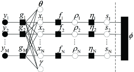
Figure 4: Factor graph of the joint distribution $p\left(\boldsymbol{v},\boldsymbol{y}\right)$.

TABLE I: Factors, Distributions and Functional forms in Fig. 4. $\mathbf{F}_{m}\left(\boldsymbol{\theta}\right)$ denotes the $m\textrm{-th}$ row of $\mathbf{F}\left(\boldsymbol{\theta}\right)$.

Factor	Distribution	Functional form
$g_{m}$	$p\left(y_{m}\mid\boldsymbol{x},\gamma,\boldsymbol{\theta}\right)$	$\mathcal{CN}\left(y_{m};\mathbf{F}_{m}\left(\boldsymbol{\theta}\right)\boldsymbol{x},\gamma^{-1}\right)$
$f_{n}$	$p\left(x_{n}\mid\rho_{n}\right)$	$\mathcal{CN}\left(x_{n};0,\rho_{n}^{-1}\right)$
$\eta_{n}$	$p\left(\rho_{n}\mid s_{n}\right)$	$\begin{cases}\textrm{Ga}\left(\rho_{n};a_{n},b_{n}\right),&s_{n}=1\\ \textrm{Ga}\left(\rho_{n};\overline{a}_{n},\overline{b}_{n}\right),&s_{n}=0\end{cases}$
$\phi$	$p\left(\boldsymbol{s};\epsilon\right)$	depends on application

For many practical applications in wireless communications, the sparse signal $\boldsymbol{x}$ usually has complicated sparse structures. For example, in our considered scenario for 6G-based target localization (Subsection II-D), a large target can be viewed as a cluster of target points [21]. In this case, the non-zero elements of the position-domain channel vector are concentrated on a few bursts. And thus, the position-domain channel exhibits a 2-D burst sparsity [33]. By exploiting this structured sparsity, we can further enhance the performance of target localization. Some recent works also exploited different structured sparsities during algorithm design. In [20][34], the authors used a Markov chain model to describe the burst sparsity of the angular-domain channel and improved the performance of channel estimation significantly. Besides, the authors in [35, 36] exploited the temporal correlation of the support set of angular-domain channels. Motivated by these, it is essential to extend our proposed IFSLA-VBI algorithm from an independent sparse prior to more complicated structured sparse priors.

IV-A Turbo-IFSLA-VBI Algorithm

Consider a more general distribution for the support vector, denoted by $p\left(\boldsymbol{s};\epsilon\right)$, where $\epsilon$ denotes the prior parameters. We can choose a proper $p\left(\boldsymbol{s};\epsilon\right)$ to model different sparse structures in practical applications. The factor graph of the joint distribution $p\left(\boldsymbol{v},\boldsymbol{y}\right)$ is shown in Fig. 4, while the associated factor nodes are listed in Table I. Due to the complicated internal structure of $\boldsymbol{s}$, the factor graph usually contains loops. In this case, exact Bayesian inference is known to be NP-hard [37].

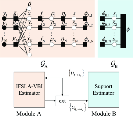
Figure 5: The turbo approach yields a decoupled factor graph and the framework of the Turbo-IFSLA-VBI algorithm.

Inspired by the turbo approach [18], we propose a Turbo-IFSLA-VBI algorithm by combining the IFSLA-VBI estimator with message passing. We first partition the factor graph in Fig. 4 along the dash line into two decoupled subgraphs, denoted by $\mathcal{G}_{\mathrm{A}}$ and $\mathcal{G}_{\mathrm{B}}$, respectively, as shown in Fig. 5. To be more specific, $\mathcal{G}_{\mathrm{A}}$ describes the internal structure of hidden variables with an independent sparse prior, while $\mathcal{G}_{\mathrm{B}}$ describes the more complicated internal structure of the support vector. Then we design Module A and Module B to perform Bayesian inference over the two subgraphs, respectively. For $\mathcal{G}_{\mathrm{A}}$, we adopt the proposed IFSLA-VBI estimator to compute each variational distribution approximately. For $\mathcal{G}_{\mathrm{B}}$, we perform message passing to compute the marginal posterior of $\boldsymbol{s}$. The two modules need to work alternately and exchange extrinsic messages until converge to a stationary point. And the output messages of one module form the priors for another module. Specifically, the extrinsic messages from Module A to B are denoted by $\left\{\upsilon_{\eta_{n}\rightarrow s_{n}}\right\}$, while the extrinsic messages from Module B to A are denoted by $\left\{\upsilon_{\phi\rightarrow s_{n}}\right\}$. Formally, we define two turbo-iteration factor nodes:

$$\phi_{\mathrm{A},n}\left(s_{n}\right) \triangleq\upsilon_{\phi\rightarrow s_{n}}\left(s_{n}\right),n=1,\ldots,N,$$ (48)

$$\phi_{\mathrm{B},n}\left(s_{n}\right) \triangleq\upsilon_{\eta_{n}\rightarrow s_{n}}\left(s_{n}\right),n=1,\ldots,N,$$

where $\phi_{\mathrm{A},n}\left(s_{n}\right)$ can be viewed as the prior information for Module A. And for each turbo iteration, the extrinsic message $\upsilon_{\eta_{n}\rightarrow s_{n}}\left(s_{n}\right)$ from Module A to B can be computed by subtracting the prior information $\phi_{\mathrm{A},n}\left(s_{n}\right)$ from posterior information,

$$\upsilon_{\eta_{n}\rightarrow s_{n}}\left(s_{n}\right)\varpropto q\left(s_{n}\right)/\phi_{\mathrm{A},n}\left(s_{n}\right),$$ (49)

where $q\left(s_{n}\right)$ is the approximate posterior distribution obtained in (27).

IV-B An Example: Markov Random Field for 2-D Burst Sparsity

To elaborate on how Module B performs message passing more clearly, we use the 6G-based target localization scenario as an example. As discussed previously, since the targets are usually distributed in clusters, the virtual position-domain channel exhibits a 2-D burst sparsity. To exploit this, we introduce a Markov random field (MRF) model [38, 33]. The support vector is modeled as

$$p\left(\boldsymbol{s}\right) =\frac{1}{Z}\exp\left(\sum_{n=1}^{N}\left(\frac{1}{2}\sum_{i\in\mathcal{N}_{n}}\beta s_{i}-\alpha\right)s_{n}\right)$$ (50)

$$=\frac{1}{Z}\left(\stackrel{{\scriptstyle[}}{{n}}=1]{N}{\prod}\underset{i\in\mathcal{N}_{n}}{\prod}\chi_{\beta}\left(s_{n},s_{i}\right)\right)^{\frac{1}{2}}\prod_{n=1}^{N}\chi_{\alpha}\left(s_{n}\right),$$

where $\chi_{\alpha}\left(s_{n}\right)\triangleq\exp\left(-\alpha s_{n}\right)$, $\chi_{\beta}\left(s_{n},s_{i}\right)\triangleq\exp\left(\beta s_{n}s_{i}\right)$, $\mathcal{N}_{n}$ is the index set of the neighbor nodes of $s_{n}$, and $Z$ is the partition function. The parameter $\alpha$ controls the degree of sparsity and the parameter $\beta$ affects the size of non-zero bursts.

Figure 6: The factor graph of the 4-connected MRF model.

We give the factor graph of the MRF model in Fig. 6, where $\left\{s_{n}\right\}_{n=1}^{N}$ denote variables nodes and $\left\{\chi_{\alpha},\chi_{\beta}\right\}$ denote factor nodes. Consider a variable node $s_{n}$, the left, right, top, and bottom neighboring variable nodes of $s_{n}$ are represented as $s_{n_{l}}$, $s_{n_{r}}$, $s_{n_{t}}$, and $s_{n_{b}}$, respectively. To simplify the notation, we use $\pi_{n}^{in}$ to abbreviate $\phi_{\mathrm{B},n}\left(s_{n}=1\right)$ for $n=1,\ldots,N$. In the following, we obey the sum-product rule to derive messages over the factor graph [39].

For $s_{n}$, the input messages from the left, right, top, and bottom neighbor nodes, denoted by $\upsilon_{n}^{l}$, $\upsilon_{n}^{r}$, $\upsilon_{n}^{t}$, and $\upsilon_{n}^{b}$, respectively, follow Bernoulli distributions, where $\upsilon_{n}^{l}$ is given by

$$\upsilon_{n}^{l} \propto\sum_{s_{n_{l}}}\upsilon_{\eta_{n_{l}}\rightarrow s_{n_{l}}}\prod_{k\in\left\{l,t,b\right\}}\upsilon{}_{n_{l}}^{k}\chi_{\alpha}\left(s_{n_{l}}\right)\chi_{\beta}\left(s_{n},s_{n_{l}}\right)$$

$$\propto\kappa_{n}^{l}\delta\left(s_{n}-1\right)+(1-\kappa_{n}^{l})\delta\left(s_{n}\right),$$ (51)

where

$$\kappa_{n}^{l}=\tfrac{\pi_{n_{l}}^{in}\prod_{k\in\left\{l,t,b\right\}}\kappa_{n_{l}}^{k}e^{-\alpha+\beta}+\left(1-\pi_{n_{l}}^{in}\right)\prod_{k\in\left\{l,t,b\right\}}\left(1-\kappa_{n_{l}}^{k}\right)e^{\alpha-\beta}}{\left(e^{\beta}+e^{-\beta}\right)\left(\pi_{n_{l}}^{in}e^{-\alpha}\prod_{k\in\left\{l,t,b\right\}}\kappa_{q_{l}}^{k}+\left(1-\pi_{n_{l}}^{in}\right)e^{\alpha}\prod_{k\in\left\{l,t,b\right\}}\left(1-\kappa_{n_{l}}^{k}\right)\right)}.$$

The messages $\upsilon_{n}^{r}$, $\upsilon_{n}^{t}$, and $\upsilon_{n}^{b}$ can be calculated in a similar way.

Then the output message for $s_{n}$ (i.e., the extrinsic message from Module B to A) can be calculated as

$$\upsilon_{\phi\rightarrow s_{n}} \propto\Pi_{k\in\left\{l,r,t,b\right\}}\upsilon_{n}^{k}\chi_{\alpha}\left(s_{n_{l}}\right)$$

$$\propto\pi_{n}^{out}\delta\left(s_{n}-1\right)+\left(1-\pi_{n}^{out}\right)\delta\left(s_{n}\right)$$ (52)

where

$$\pi_{n}^{out}=\frac{e^{-\alpha}\Pi_{k\in\left\{l,r,t,b\right\}}\kappa_{n}^{k}}{e^{-\alpha}\Pi_{k\in\left\{l,r,t,b\right\}}\kappa_{n}^{k}+e^{\alpha}\Pi_{k\in\left\{l,r,t,b\right\}}\left(1-\kappa_{n}^{k}\right)}.$$

IV-C Summary of the Turbo-IFSLA-VBI

We summarize the Turbo-IFSLA-VBI algorithm in Algorithm 3. Since the message passing is usually linear complexity, the additional computational overhead caused by Module B is almost negligible.

Algorithm 3 Turbo-IFSLA-VBI algorithm

Input: $\boldsymbol{y}$, initial grid $\overline{\boldsymbol{\theta}}$, iteration number $I=I_{1}+I_{2}$ ($I_{2}=I_{\textrm{A}}I_{\textrm{B}}$), local iteration number $T$.

Output: $\boldsymbol{x}^{*}$, $\boldsymbol{s}^{*}$, and $\boldsymbol{\theta}^{*}$.

1:  % Stage 1: Initialization

2:  Same as the initialization stage of the IFSLA-VBI.

3:  % Stage 2: Turbo-IFSLA-VBI Algorithm

4:  for ${\color[rgb]{0,0,1}{\color[rgb]{0,0,0}i_{b}=1,\cdots,I_{\textrm{B}}}}$ do

5:     % Module A: IFSLA-VBI Estimator

6:     Initialize $i_{a}=1$.

7:     while not converge and $i_{a}\leq I_{\textrm{A}}$ do

8:        Optimize $q\left(\boldsymbol{x}\right)$, $q\left(\boldsymbol{\rho}\right)$, $q\left(\boldsymbol{s}\right)$, $q\left(\gamma\right)$, and $q\left(\boldsymbol{\theta}\right)$ alternatively according to the IFSLA-VBI algorithm.

9:        $i_{a}=i_{a}+1$.

10:     end while

11:     Compute $\left\{\upsilon_{\eta_{n}\rightarrow s_{n}}\right\}$ based on (49) and send it to Module B.

12:     % Module B: Support Estimator

13:     Perform message passing over $\mathcal{G}_{\mathrm{B}}$, send $\left\{\upsilon_{\phi\rightarrow s_{n}}\right\}$ to Module A.

14:  end for

15:  Output $\boldsymbol{x}^{*}=\boldsymbol{\mu}_{x}$, $s_{n}^{*}=\widetilde{\lambda}_{n},\forall n$, and $\mathbf{\boldsymbol{\theta}^{\mathit{j}}}^{*}=\boldsymbol{\mu}_{\theta^{j}},\forall j$.

V Simulation Results

In this section, we apply the proposed algorithm to solve two practical application problems and verify its advantages compared to other baselines. Different algorithms are elaborated below.

TABLE II: Complexity order, numerical value of order, and CPU time for different algorithms

Algorithms	Complexity order	Numerical value of order		CPU time
		Application 1	Application 2	Application 1	Application 2
OGSBI	$\Theta\left(IN^{3}\right)$	$\Theta\left(1.0\times 10^{8}\right)$	$\Theta\left(6.7\times 10^{9}\right)$	0.0561s
SBL/EM	$\Theta\left(I_{out}I_{in}N^{3}+I_{out}N^{2}M\right)$	$\Theta\left(1.1\times 10^{9}\right)$	$\Theta\left(7.4\times 10^{10}\right)$	0.433s	25.3s
Turbo-CS/EM	$\Theta\left(I_{out}I_{in}N^{3}+I_{out}N^{2}M\right)$	$\Theta\left(1.1\times 10^{9}\right)$	$\Theta\left(7.4\times 10^{10}\right)$	0.449s	18.4s
Turbo-VBI/EM	$\Theta\left(I_{out}I_{in}N^{3}+I_{out}N^{2}M\right)$	$\Theta\left(1.1\times 10^{9}\right)$	$\Theta\left(7.4\times 10^{10}\right)$	0.453s	25.4s
SLA-VBI	$\Theta\left(I\left(2N^{3}+N^{2}M+BN^{2.375}\right)\right)$	$\Theta\left(2.6\times 10^{8}\right)$	$\Theta\left(2.0\times 10^{10}\right)$	0.185s
IFSLA-VBI	$\Theta\left(I\left(2N^{2}T+N^{2}M+BN^{2.375}\right)\right)$	$\Theta\left(7.4\times 10^{7}\right)$	$\Theta\left(7.2\times 10^{9}\right)$	0.0550s	2.00s
Turbo-IFSLA-VBI	$\Theta\left(I\left(2N^{2}T+N^{2}M+BN^{2.375}\right)\right)$	$\Theta\left(7.4\times 10^{7}\right)$	$\Theta\left(7.2\times 10^{9}\right)$		2.02s

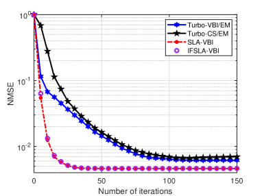
Figure 7: Convergence behavior of the Turbo-VBI, Turbo-CS, SLA-VBI, and IFSLA-VBI. The number of pilot sequences is set to $64$ and SNR is 10 dB.

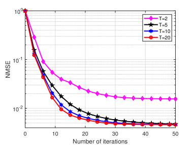
Figure 8: Convergence behavior of the IFSLA-VBI algorithm with different local iteration numbers. We set $T=2,5,10,20$.

• OGSBI [15]: It is a single-loop algorithm based on linear approximation.

• EM-based sparse Bayesian learning (SBL) [12]: It is a double-loop EM framework, where the E-step applies a SBL estimator to recover sparse signals and the M-step uses a gradient ascent method to update dynamic grid parameters.

• EM-based Turbo-CS [19, 20, 21]: It is a double-loop EM framework, where the E-step is the Turbo-CS algorithm and the M-step performs gradient ascent update.

• EM-based Turbo-VBI [22, 23]: It is a double-loop EM framework, where the E-step is the Turbo-VBI algorithm and the M-step performs gradient ascent update.

• SLA-VBI: The proposed SLA-VBI algorithm is single-loop but involves two complicated matrix inverse operations in each iteration.

• IFSLA-VBI: It is the simplified version of the SLA-VBI, where the matrix inverse is approximated by the MM framework.

• Turbo-IFSLA-VBI: It is the extension of the IFSLA-VBI, which can exploit different sparse structures.

For the OGSBI and our proposed algorithms, the maximum number of iterations is set to $I=50$. For the double-loop EM-based algorithms, the inner iteration number of the Bayesian estimator is set to $I_{in}=10$ and the outer iteration number of the EM is set to $I_{out}=50$. For the IFSLA-VBI and Turbo-IFSLA-VBI, the number of iterations used to approximate the matrix inverse is set to $T=10$. As seen from Table II, both the complexity order and the average run time of the proposed IFSLA-VBI are significantly lower than the double-loop EM-based methods . The source code is available at https://github.com/ZJU-XWK/SLA-VBI.

V-A Massive MIMO Channel Estimation

V-A1 Implementation Details

In the simulations, the BS is equipped with a ULA of $128$ antennas. The pilot symbols are generated with random phase under unit power constrains. The number of AoD grid points is set to $128$. For the three-layer sparse prior model, we set $a_{n}=1$, $b_{n}=1$, $\overline{a}_{n}=1$, $\overline{b}_{n}=10^{-5}$, $c=10^{-6}$, and $d=10^{-6}$. We choose the normalized mean square error (NMSE) as the performance metric for channel estimation. The related parameters for simulations are listed in Table III.

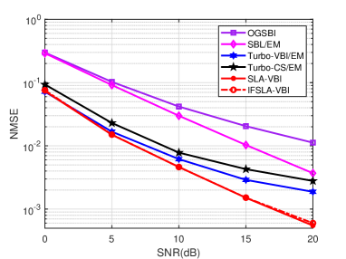
Figure 9: The NMSE performance of the channel estimation versus SNR. The number of pilot sequences is $64$.

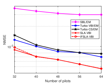
Figure 10: The NMSE performance of the channel estimation versus number of pilot sequences. We set $\textrm{SNR}=10~{}\textrm{dB}$.

V-A2 Convergence Behavior

In Fig. 8, we compare the convergence behavior of different algorithms. The proposed IFSLA-VBI has a much faster convergence speed than the double-loop EM-based Turbo-CS and Turbo-VBI. Besides, the IFSLA-VBI has similar convergence behavior to the more complicated SLA-VBI, which reflects that the matrix inverse approximated by the local iterations is accurate enough. In Fig. 8, we change the number of local iterations used to approximate the matrix inverse and evaluate the convergence behavior of the IFSLA-VBI algorithm. As can be seen, the IFSLA-VBI still works well for $T$ as small as $5$. That is to say, the IFSLA-VBI can achieve comparable performance to the SLA-VBI while greatly reducing the computational overhead.

V-A3 Influence of SNR

In Fig. 9, we show the performance of channel estimation versus SNR. It can be seen that the performance of all the algorithms improves as the SNR increases. With limited training sequences, the OGSBI works poorly. Besides, the EM-based Turbo-VBI works better than the EM-based SBL, which reflects the advantage of the three-layer sparse prior model used in Turbo-VBI. Furthermore, the proposed IFSLA-VBI can achieve a significant performance gain over the state-of-the-art Turbo-CS and Turbo-VBI, especially in the high SNR regions. This is because the proposed IFSLA-VBI can output Bayesian estimation of both sparse signals and grid parameters but the EM-based methods can only provide a point estimation of grid parameters. Finally, the curves of the IFSLA-VBI and SLA-VBI almost overlap, i.e., they have almost the same performance.

V-A4 Influence of Number of Pilots

In Fig. 10, we focus on how the number of pilot sequences affects the performance of channel estimation. As the number of pilot sequences increases, the performance of all the algorithms improves. And it is obvious that the proposed IFSLA-VBI still performs better than the EM-based methods.

TABLE III: Related parameters for simulations

Application 1		Application 2
Parameter	Value	Parameter	Value
Antenna number	128	Antenna number	64
Pilot number	64	RF chain number	16
AoD grid points	128	Subcarrier number	1024
		Subcarrier interval	$30~{}\textrm{kHz}$
		Position grid points	512

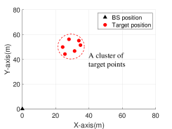
(a) The 2-D platform.

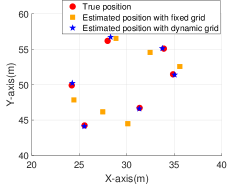
(b) Target localization result.

Figure 11: Illustration of the simulation setup for 6G-based target localization.

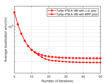
Figure 12: Convergence behavior of the Turbo-IFSLA-VBI with an i.i.d. prior and the MRF prior. We set $\textrm{SNR}=0~{}\textrm{dB}$.

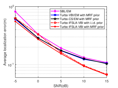
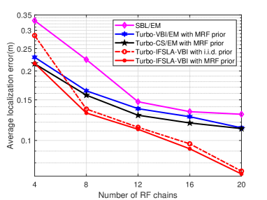
Figure 13: Average localization error versus SNR. The number of RF chains is $16$.

Figure 14: Average localization error versus number of RF chains. We set $\textrm{SNR}=10~{}\textrm{dB}$.

V-B 6G-based Target Localization

V-B1 Implementation Details

We consider a 2-D platform, where the BS is deployed at the corner with the coordinates $\left(0~{}\textrm{m},0~{}\textrm{m}\right)$ and the targets are concentrated in a cluster, as shown in Fig. 11a. The BS has $64$ antennas and $16$ RF chains. The number of OFDM subcarriers is set to $1024$ and the subcarrier interval is $30~{}\textrm{kHz}$. Probing signals are generated with random phase under unit power constrains, and they are inserted at intervals of $32$ OFDM subcarriers, i.e., $\left|\mathcal{N}_{b}\right|=\tfrac{1024}{32}=32$. The RF combining matrix $\mathbf{W}_{\textrm{RF}}$ is partially orthogonal. The model parameters of the MRF is set to $\alpha=0.3$ and $\beta=0.5$. We introduce a position-domain dynamic grid with $512$ grid points for target localization. The simulation parameters are listed in Table III. The dynamic grid will greatly improve localization accuracy, as shown in Fig. 11b. In contrast, there is a glaring mismatch between the true positions and the estimated positions when using a fixed sampling grid.

V-B2 Convergence Behavior

In Fig. 12, we compare the convergence behavior of the proposed Turbo-IFSLA-VBI algorithm with different sparse priors. It can be seen that the algorithm with the MRF prior has a much smaller localization error after convergence. This indicates that the proposed Turbo-IFSLA-VBI has the ability to utilize the structured sparse prior information to improve the performance.

V-B3 Influence of SNR

In Fig. 14, we evaluate the performance of target localization versus SNR. The proposed Turbo-IFSLA-VBI with the MRF prior has the smallest localization error among all the algorithms. There is a significant performance gap between the Turbo-IFSLA-VBI with the MRF prior and the same algorithm with an i.i.d. prior, which reflects that the MRF prior can fully exploit the 2-D burst sparsity of the position-domain channel. In the high SNR regions, the localization error of the EM-based methods is much larger than our proposed algorithm, which reflects the advantage of Bayesian estimation of grid parameters.

V-B4 Influence of Number of RF Chains

In Fig. 14, we evaluate the performance of target localization versus number of RF chains. Again, the proposed Turbo-IFSLA-VBI with the MRF prior achieves the best performance.

VI Conclusion

We propose a novel SLA-VBI algorithm to recover a structured sparse signal from a linear model with uncertain grid parameters in the sensing matrix. In contrast to conventional EM-based methods, our proposed algorithm can provide approximate posterior distribution of both sparse signals and dynamic grid parameters. To reduce the computational overhead caused by the matrix inverse, we design an inverse-free algorithm (i.e., IFSLA-VBI) based on the MM framework. And then we extend the proposed algorithm from an independent sparse prior to more complicated structured sparse priors by using the turbo approach. Finally, we apply our proposed algorithm to solve two practical applications, i.e., massive MIMO channel estimation and 6G-based target localization. The simulations verify that our proposed algorithm can achieve faster convergence, lower complexity, and better performance compared to the state-of-the-art EM-based methods.

-A Derivation of (38) - (40)

Substituting (34) into (32) and ignoring the terms that are not related to $\boldsymbol{\theta}^{j}$, $q\left(\boldsymbol{\theta}^{j}\right)$ can be derived as

$$\ln q\left(\boldsymbol{\theta}^{j}\right)\propto \left\langle\ln p\left(\boldsymbol{y}\mid\boldsymbol{x},\boldsymbol{\theta},\gamma\right)\right\rangle_{q\left(\boldsymbol{x}\right)q\left(\gamma\right)\Pi_{i\neq j}q\left(\boldsymbol{\theta}^{i}\right)}+\ln p\left(\boldsymbol{\theta}^{j}\right)$$

$$\propto -\left\langle\gamma\right\rangle\left\langle\left\|\boldsymbol{y}-\overline{\mathbf{F}}\left(\boldsymbol{\theta}\right)\boldsymbol{x}\right\|^{2}\right\rangle_{q\left(\boldsymbol{x}\right)\Pi_{i\neq j}q\left(\boldsymbol{\theta}^{i}\right)}$$

$$+\ln\mathcal{N}\left(\boldsymbol{\theta}^{j};\overline{\boldsymbol{\theta}}^{j},1/\kappa^{j}\mathbf{I}_{N}\right)$$

$$\propto -\left\langle\gamma\right\rangle\left\langle\left\|\boldsymbol{y}-\overline{\mathbf{F}}\left(\boldsymbol{\theta}\right)\boldsymbol{\mu}_{x}\right\|^{2}\right\rangle_{\Pi_{i\neq j}q\left(\boldsymbol{\theta}^{i}\right)}$$

$$-\left\langle\gamma\right\rangle\left\langle\textrm{Tr}\left(\overline{\mathbf{F}}\left(\boldsymbol{\theta}\right)\boldsymbol{\Sigma}_{x}\overline{\mathbf{F}}\left(\boldsymbol{\theta}\right)^{H}\right)\right\rangle_{\Pi_{i\neq j}q\left(\boldsymbol{\theta}^{i}\right)}$$

$$+\ln\mathcal{N}\left(\boldsymbol{\theta}^{j};\overline{\boldsymbol{\theta}}^{j},1/\kappa^{j}\mathbf{I}_{N}\right)$$

$$\propto -\left\langle\gamma\right\rangle\boldsymbol{\mu}_{x}^{H}\left\langle\overline{\mathbf{F}}\left(\boldsymbol{\theta}\right)^{H}\overline{\mathbf{F}}\left(\boldsymbol{\theta}\right)\right\rangle_{\Pi_{i\neq j}q\left(\boldsymbol{\theta}^{i}\right)}\boldsymbol{\mu}_{x}$$

$$+2\left\langle\gamma\right\rangle\mathfrak{Re}\left\{\boldsymbol{\mu}_{x}^{H}\left\langle\overline{\mathbf{F}}\left(\boldsymbol{\theta}\right)^{H}\right\rangle_{\Pi_{i\neq j}q\left(\boldsymbol{\theta}^{i}\right)}\boldsymbol{y}\right\}$$

$$-\left\langle\gamma\right\rangle\textrm{Tr}\left(\left\langle\overline{\mathbf{F}}\left(\boldsymbol{\theta}\right)^{H}\overline{\mathbf{F}}\left(\boldsymbol{\theta}\right)\right\rangle_{\Pi_{i\neq j}q\left(\boldsymbol{\theta}^{i}\right)}\boldsymbol{\Sigma}_{x}\right)$$

$$+\ln\mathcal{N}\left(\boldsymbol{\theta}^{j};\overline{\boldsymbol{\theta}}^{j},1/\kappa^{j}\mathbf{I}_{N}\right),$$ (53)

The first term in (53) can be computed as

$$\textrm{Term1}= -\left\langle\gamma\right\rangle\boldsymbol{\mu}_{x}^{H}\left\langle\overline{\mathbf{F}}\left(\boldsymbol{\theta}\right)^{H}\overline{\mathbf{F}}\left(\boldsymbol{\theta}\right)\right\rangle_{\Pi_{i\neq j}q\left(\boldsymbol{\theta}^{i}\right)}\boldsymbol{\mu}_{x}$$

$$= -2\left\langle\gamma\right\rangle\boldsymbol{\mu}_{x}^{H}\mathfrak{Re}\left\{\textrm{diag}\left(\boldsymbol{\theta}^{j}-\hat{\boldsymbol{\mu}}_{\theta^{j}}\right)\mathbf{A^{\mathit{j}}}^{H}\mathbf{F}\left(\hat{\boldsymbol{\mu}}_{\theta}\right)\right\}\boldsymbol{\mu}_{x}$$

$$-\left\langle\gamma\right\rangle\boldsymbol{\mu}_{x}^{H}\textrm{diag}\left(\boldsymbol{\theta}^{j}-\hat{\boldsymbol{\mu}}_{\theta^{j}}\right)\mathbf{A^{\mathit{j}}}^{H}\mathbf{A^{\mathit{j}}}\textrm{diag}\left(\boldsymbol{\theta}^{j}-\hat{\boldsymbol{\mu}}_{\theta^{j}}\right)\boldsymbol{\mu}_{x}$$

$$= -2\left\langle\gamma\right\rangle\mathfrak{Re}\left\{\boldsymbol{\mu}_{x}^{H}\textrm{diag}\left(\boldsymbol{\theta}^{j}-\hat{\boldsymbol{\mu}}_{\theta^{j}}\right)\mathbf{A^{\mathit{j}}}^{H}\mathbf{F}\left(\hat{\boldsymbol{\mu}}_{\theta}\right)\boldsymbol{\mu}_{x}\right\}$$

$$-\left\langle\gamma\right\rangle\mathfrak{Re}\Bigl{\{}\left(\boldsymbol{\theta}^{j}-\hat{\boldsymbol{\mu}}_{\theta^{j}}\right)^{T}$$

$$\hskip 17.07182pt\left[\textrm{diag}\left(\boldsymbol{\mu}_{x}\right)^{H}\mathbf{A^{\mathit{j}}}^{H}\mathbf{A^{\mathit{j}}}\textrm{diag}\left(\boldsymbol{\mu}_{x}\right)\right]\left(\boldsymbol{\theta}^{j}-\hat{\boldsymbol{\mu}}_{\theta^{j}}\right)\Bigr{\}}$$

$$= -2\left\langle\gamma\right\rangle\mathfrak{Re}\left\{\left(\boldsymbol{\theta}^{j}-\hat{\boldsymbol{\mu}}_{\theta^{j}}\right)^{T}\textrm{diag}\left(\boldsymbol{\mu}_{x}\right)^{H}\mathbf{A^{\mathit{j}}}^{H}\mathbf{F}\left(\hat{\boldsymbol{\mu}}_{\theta}\right)\boldsymbol{\mu}_{x}\right\}$$

$$-\left\langle\gamma\right\rangle\left(\boldsymbol{\theta}^{j}-\hat{\boldsymbol{\mu}}_{\theta^{j}}\right)^{T}$$

$$\hskip 17.07182pt\mathfrak{Re}\left\{\left(\boldsymbol{\mu}_{x}\boldsymbol{\mu}_{x}^{H}\right)^{T}\odot\left(\mathbf{A^{\mathit{j}}}^{H}\mathbf{A^{\mathit{j}}}\right)\right\}\left(\boldsymbol{\theta}^{j}-\hat{\boldsymbol{\mu}}_{\theta^{j}}\right).$$ (54)

The second term in (53) can be computed as

Term2 $$=2\left\langle\gamma\right\rangle\mathfrak{Re}\left\{\boldsymbol{\mu}_{x}^{H}\left\langle\overline{\mathbf{F}}\left(\boldsymbol{\theta}\right)^{H}\right\rangle_{\Pi_{i\neq j}q\left(\boldsymbol{\theta}^{i}\right)}\boldsymbol{y}\right\}$$

$$=2\left\langle\gamma\right\rangle\mathfrak{Re}\left\{\boldsymbol{\mu}_{x}^{H}\textrm{diag}\left(\boldsymbol{\theta}^{j}-\hat{\boldsymbol{\mu}}_{\theta^{j}}\right)\mathbf{A^{\mathit{j}}}^{H}\boldsymbol{y}\right\}$$

$$=2\left\langle\gamma\right\rangle\mathfrak{Re}\left\{\left(\boldsymbol{\theta}^{j}-\hat{\boldsymbol{\mu}}_{\theta^{j}}\right)^{T}\textrm{diag}\left(\boldsymbol{\mu}_{x}\right)^{H}\mathbf{A^{\mathit{j}}}^{H}\boldsymbol{y}\right\}.$$ (55)

The third term in (53) can be computed as

Term3= $$-\left\langle\gamma\right\rangle\textrm{Tr}\left(\left\langle\overline{\mathbf{F}}\left(\boldsymbol{\theta}\right)^{H}\overline{\mathbf{F}}\left(\boldsymbol{\theta}\right)\right\rangle_{\Pi_{i\neq j}q\left(\boldsymbol{\theta}^{i}\right)}\boldsymbol{\Sigma}_{x}\right)$$

$$= -\left\langle\gamma\right\rangle\textrm{Tr}\left(2\mathfrak{Re}\left\{\textrm{diag}\left(\boldsymbol{\theta}^{j}-\hat{\boldsymbol{\mu}}_{\theta^{j}}\right)\mathbf{A^{\mathit{j}}}^{H}\mathbf{F}\left(\hat{\boldsymbol{\mu}}_{\theta}\right)\boldsymbol{\Sigma}_{x}\right\}\right)$$

$$-\left\langle\gamma\right\rangle\mathfrak{Re}\Bigl{\{}\textrm{Tr}\Bigl{(}\textrm{diag}\left(\boldsymbol{\theta}^{j}-\hat{\boldsymbol{\mu}}_{\theta^{j}}\right)$$

$$\hskip 28.45274pt\mathbf{A^{\mathit{j}}}^{H}\mathbf{A^{\mathit{j}}}\textrm{diag}\left(\boldsymbol{\theta}^{j}-\hat{\boldsymbol{\mu}}_{\theta^{j}}\right)\boldsymbol{\Sigma}_{x}\Bigr{)}\Bigr{\}}$$

$$= -\left\langle\gamma\right\rangle 2\mathfrak{Re}\left\{\left(\boldsymbol{\theta}^{j}-\hat{\boldsymbol{\mu}}_{\theta^{j}}\right)^{T}\textrm{diag}\left(\mathbf{A^{\mathit{j}}}^{H}\mathbf{F}\left(\hat{\boldsymbol{\mu}}_{\theta}\right)\boldsymbol{\Sigma}_{x}\right)\right\}$$

$$-\left\langle\gamma\right\rangle\mathfrak{Re}\Bigl{\{}\left(\boldsymbol{\theta}^{j}-\hat{\boldsymbol{\mu}}_{\theta^{j}}\right)^{T}$$

$$\hskip 28.45274pt\textrm{diag}\left(\mathbf{A^{\mathit{j}}}^{H}\mathbf{A^{\mathit{j}}}\textrm{diag}\left(\boldsymbol{\theta}^{j}-\hat{\boldsymbol{\mu}}_{\theta^{j}}\right)\boldsymbol{\Sigma}_{x}\right)\Bigr{\}}$$

$$= -\left\langle\gamma\right\rangle 2\mathfrak{Re}\left\{\left(\boldsymbol{\theta}^{j}-\hat{\boldsymbol{\mu}}_{\theta^{j}}\right)^{T}\textrm{diag}\left(\mathbf{A^{\mathit{j}}}^{H}\mathbf{F}\left(\hat{\boldsymbol{\mu}}_{\theta}\right)\boldsymbol{\Sigma}_{x}\right)\right\}$$

$$-\left\langle\gamma\right\rangle\left(\boldsymbol{\theta}^{j}-\hat{\boldsymbol{\mu}}_{\theta^{j}}\right)^{T}\mathfrak{Re}\left\{\boldsymbol{\Sigma}_{x}^{T}\odot\mathbf{A^{\mathit{j}}}^{H}\mathbf{A^{\mathit{j}}}\right\}\left(\boldsymbol{\theta}^{j}-\hat{\boldsymbol{\mu}}_{\theta^{j}}\right).$$ (56)

Substituting (54), (55), and (56) into (53), we have

$$\ln q\left(\boldsymbol{\theta}^{j}\right)\propto -\frac{1}{2}\left(\boldsymbol{\theta}^{j}-\hat{\boldsymbol{\mu}}_{\theta^{j}}\right)^{T}\left\langle\gamma\right\rangle\mathbf{H}_{\theta^{j}}\left(\boldsymbol{\theta}^{j}-\hat{\boldsymbol{\mu}}_{\theta^{j}}\right)$$

$$+\left(\boldsymbol{\theta}^{j}-\hat{\boldsymbol{\mu}}_{\theta^{j}}\right)^{T}\left\langle\gamma\right\rangle\boldsymbol{g}_{\theta^{j}}$$

$$+\ln\mathcal{N}\left(\boldsymbol{\theta}^{j};\overline{\boldsymbol{\theta}}^{j},1/\kappa^{j}\mathbf{I}_{N}\right)+\textrm{const}$$

$$\propto \ln\mathcal{N}\left(\boldsymbol{\theta}^{j};\mathbf{H}_{\theta^{j}}^{-1}\boldsymbol{g}_{\theta^{j}}+\hat{\boldsymbol{\mu}}_{\theta^{j}},\left\langle\gamma\right\rangle^{-1}\mathbf{H}_{\theta^{j}}^{-1}\right)$$

$$+\ln\mathcal{N}\left(\boldsymbol{\theta}^{j};\overline{\boldsymbol{\theta}}^{j},1/\kappa^{j}\mathbf{I}_{N}\right)+\textrm{const}$$

$$\propto \ln\mathcal{N}\left(\boldsymbol{\theta}^{j};\boldsymbol{\mu}_{\theta^{j}},\boldsymbol{\Sigma}_{\theta^{j}}\right),\forall j,$$ (57)

where the immediate variables has been defined to simplify notations:

$$\mathbf{H}_{\theta^{j}}= 2\mathfrak{Re}\left\{\left(\boldsymbol{\mu}_{x}\boldsymbol{\mu}_{x}^{H}+\boldsymbol{\Sigma}_{x}\right)^{T}\odot\left(\mathbf{A^{\mathit{j}}}^{H}\mathbf{A^{\mathit{j}}}\right)\right\},\forall j,$$ (58)

$$\boldsymbol{g}_{\theta^{j}}= 2\mathfrak{Re}\left\{\textrm{diag}\left(\boldsymbol{\mu}_{x}\right)^{H}\mathbf{A^{\mathit{j}}}^{H}\left(\boldsymbol{y}-\mathbf{F}\left(\hat{\boldsymbol{\mu}}_{\theta}\right)\boldsymbol{\mu}_{x}\right)\right\}$$

$$-2\mathfrak{Re}\left\{\textrm{diag}\left(\mathbf{A^{\mathit{j}}}^{H}\mathbf{F}\left(\hat{\boldsymbol{\mu}}_{\theta}\right)\boldsymbol{\Sigma}_{x}\right)\right\},\forall j,$$

and the approximate posterior mean and covariance matrix of $\boldsymbol{\theta}^{j}$ are respectively given by

$$\boldsymbol{\mu}_{\theta^{j}} =\boldsymbol{\Sigma}_{\theta^{j}}\left(\left\langle\gamma\right\rangle\left(\boldsymbol{g}_{\theta^{j}}+\mathbf{H}_{\theta^{j}}\hat{\boldsymbol{\mu}}_{\theta^{j}}\right)+\kappa^{j}\overline{\boldsymbol{\theta}}^{j}\right),\forall j,$$ (59)

$$\boldsymbol{\Sigma}_{\theta^{j}} =\left(\left\langle\gamma\right\rangle\mathbf{H}_{\theta^{j}}+\kappa^{j}\mathbf{I}_{N}\right)^{-1},\forall j.$$

References

• [1] C. R. Berger, Z. Wang, J. Huang, and S. Zhou, “Application of compressive sensing to sparse channel estimation,” IEEE Commun. Mag., vol. 48, no. 11, pp. 164–174, 2010.
• [2] J. L. Paredes, G. R. Arce, and Z. Wang, “Ultra-wideband compressed sensing: Channel estimation,” IEEE J. Sel. Topics Signal Process., vol. 1, no. 3, pp. 383–395, 2007.
• [3] L. Cheng, C. Xing, and Y.-C. Wu, “Irregular array manifold aided channel estimation in massive MIMO communications,” IEEE J. Sel. Topics Signal Process., vol. 13, no. 5, pp. 974–988, 2019.
• [4] A. C. Cirik, N. Mysore Balasubramanya, and L. Lampe, “Multi-user detection using ADMM-based compressive sensing for uplink grant-free NOMA,” IEEE Commun. Lett., vol. 7, no. 1, pp. 46–49, 2018.
• [5] R. Prasad, C. R. Murthy, and B. D. Rao, “Joint approximately sparse channel estimation and data detection in OFDM systems using sparse Bayesian learning,” IEEE Trans. Signal Process., vol. 62, no. 14, pp. 3591–3603, 2014.
• [6] B. Sun, Y. Guo, N. Li, and D. Fang, “Multiple target counting and localization using variational Bayesian EM algorithm in wireless sensor networks,” IEEE Trans. Commun., vol. 65, no. 7, pp. 2985–2998, 2017.
• [7] B. Zhang, X. Cheng, N. Zhang, Y. Cui, Y. Li, and Q. Liang, “Sparse target counting and localization in sensor networks based on compressive sensing,” in Proc. IEEE INFOCOM, 2011, pp. 2255–2263.
• [8] J. Dai, A. Liu, and V. K. N. Lau, “FDD massive MIMO channel estimation with arbitrary 2D-array geometry,” IEEE Trans. Signal Process., vol. 66, no. 10, pp. 2584–2599, 2018.
• [9] J. A. Tropp and A. C. Gilbert, “Signal recovery from random measurements via orthogonal matching pursuit,” IEEE Trans. Inf. Theory, vol. 53, no. 12, pp. 4655–4666, 2007.
• [10] D. Malioutov, M. Cetin, and A. Willsky, “A sparse signal reconstruction perspective for source localization with sensor arrays,” IEEE Trans. Signal Process., vol. 53, no. 8, pp. 3010–3022, 2005.
• [11] A. Liu, V. K. N. Lau, and W. Dai, “Exploiting burst-sparsity in massive MIMO with partial channel support information,” IEEE Trans. Wireless Commun., vol. 15, no. 11, pp. 7820–7830, 2016.
• [12] M. E. Tipping, “Sparse Bayesian learning and the relevance vector machine,” J. Mach. Learn. Res., vol. 1, no. 3, pp. 211–244, 2001.
• [13] S. Ji, Y. Xue, and L. Carin, “Bayesian compressive sensing,” IEEE Trans. Signal Process., vol. 56, no. 6, pp. 2346–2356, 2008.
• [14] S. D. Babacan, R. Molina, and A. K. Katsaggelos, “Bayesian compressive sensing using Laplace priors,” IEEE Trans. Image Process., vol. 19, no. 1, pp. 53–63, 2010.
• [15] Z. Yang, L. Xie, and C. Zhang, “Off-grid direction of arrival estimation using sparse Bayesian inference,” IEEE Trans. Signal Process., vol. 61, no. 1, pp. 38–43, 2013.
• [16] L. Xu, L. Cheng, N. Wong, Y.-C. Wu, and H. Veincent Poor, “Overcoming beam squint in dual-wideband mmwave MIMO channel estimation: A Bayesian multi-band sparsity approach,” [Online]. Available: https://arxiv.org/pdf/2306.11149.
• [17] X. Xu, M. Shen, S. Zhang, D. Wu, and D. Zhu, “Off-grid DOA estimation of coherent signals using weighted sparse Bayesian inference,” in Proc. IEEE 16th Conf. Ind. Electron. Appl. (ICIEA), 2021, pp. 1147–1150.
• [18] S. Som and P. Schniter, “Compressive imaging using approximate message passing and a Markov-tree prior,” IEEE Trans. Signal Process., vol. 60, no. 7, pp. 3439–3448, 2012.
• [19] J. Ma, X. Yuan, and L. Ping, “Turbo compressed sensing with partial DFT sensing matrix,” IEEE Signal Process. Lett., vol. 22, no. 2, pp. 158–161, 2015.
• [20] A. Liu, L. Lian, V. K. N. Lau, and X. Yuan, “Downlink channel estimation in multiuser massive MIMO with hidden Markovian sparsity,” IEEE Trans. Signal Process., vol. 66, no. 18, pp. 4796–4810, 2018.
• [21] Z. Huang, K. Wang, A. Liu, Y. Cai, R. Du, and T. X. Han, “Joint pilot optimization, target detection and channel estimation for integrated sensing and communication systems,” IEEE Trans. Wireless Commun., vol. 21, no. 12, pp. 10 351–10 365, 2022.
• [22] A. Liu, G. Liu, L. Lian, V. K. N. Lau, and M.-J. Zhao, “Robust recovery of structured sparse signals with uncertain sensing matrix: A Turbo-VBI approach,” IEEE Trans. Wireless Commun., vol. 19, no. 5, pp. 3185–3198, 2020.
• [23] A. Liu, L. Lian, V. Lau, G. Liu, and M.-J. Zhao, “Cloud-assisted cooperative localization for vehicle platoons: A turbo approach,” IEEE Trans. Signal Process., vol. 68, pp. 605–620, 2020.
• [24] Y. Sun, P. Babu, and D. P. Palomar, “Majorization-minimization algorithms in signal processing, communications, and machine learning,” IEEE Trans. Signal Process., vol. 65, no. 3, pp. 794–816, 2017.
• [25] J. A. Zhang, F. Liu, C. Masouros, R. W. Heath, Z. Feng, L. Zheng, and A. Petropulu, “An overview of signal processing techniques for joint communication and radar sensing,” IEEE J. Sel. Topics Signal Process., vol. 15, no. 6, pp. 1295–1315, 2021.
• [26] Z. Xu, A. Petropulu, and S. Sun, “A joint design of MIMO-OFDM dual-function radar communication system using generalized spatial modulation,” in Proc. IEEE Radar Conf (RadarConf20), 2020, pp. 1–6.
• [27] G. Parisi and R. Shankar, “Statistical field theory,” 1988.
• [28] D. G. Tzikas, A. C. Likas, and N. P. Galatsanos, “The variational approximation for Bayesian inference,” IEEE Signal Process. Mag., vol. 25, no. 6, pp. 131–146, 2008.
• [29] R. Danescu, F. Oniga, and S. Nedevschi, “Modeling and tracking the driving environment with a particle-based occupancy grid,” IEEE Trans. Intell. Transp. Syst., vol. 12, no. 4, pp. 1331–1342, 2011.
• [30] B. Zhou, Q. Chen, H. Wymeersch, P. Xiao, and L. Zhao, “Variational inference-based positioning with nondeterministic measurement accuracies and reference location errors,” IEEE Trans. Mobile Comput., vol. 16, no. 10, pp. 2955–2969, 2017.
• [31] H. Duan, L. Yang, J. Fang, and H. Li, “Fast inverse-free sparse Bayesian learning via relaxed evidence lower bound maximization,” IEEE Signal Process. Lett., vol. 24, no. 6, pp. 774–778, 2017.
• [32] D. Coppersmith and S. Winograd, “Matrix multiplication via arithmetic progressions,” J. Symbolic Computation, 1987.
• [33] W. Xu, Y. Xiao, A. Liu, M. Lei, and M.-J. Zhao, “Joint scattering environment sensing and channel estimation based on non-stationary Markov random field,” IEEE Trans. Wireless Commun., pp. 1–1, 2023.
• [34] L. Chen, A. Liu, and X. Yuan, “Structured turbo compressed sensing for massive MIMO channel estimation using a Markov prior,” IEEE Trans. Veh. Technol., vol. 67, no. 5, pp. 4635–4639, 2018.
• [35] Z. Gao, L. Dai, Z. Wang, and S. Chen, “Spatially common sparsity based adaptive channel estimation and feedback for FDD massive MIMO,” IEEE Trans. Signal Process., vol. 63, no. 23, pp. 6169–6183, 2015.
• [36] L. Lian, A. Liu, and V. K. N. Lau, “Exploiting dynamic sparsity for downlink FDD-massive MIMO channel tracking,” IEEE Trans. Signal Process., vol. 67, no. 8, pp. 2007–2021, 2019.
• [37] G. F. Cooper, “The computational complexity of probabilistic inference using Bayesian belief networks,” Art. Intell., vol. 42, pp. 393–405, 1990.
• [38] S. Z. Li, Markov Random Field Modeling in Image Analysis.   London, U.K.:Springer, 2009.
• [39] F. Kschischang, B. Frey, and H.-A. Loeliger, “Factor graphs and the sum-product algorithm,” IEEE Trans. Inf. Theory, vol. 47, no. 2, pp. 498–519, 2001.