Generating probability distributions using variational quantum circuits

Abstract

We use a variational method for generating probability distributions, specifically, the Uniform, the Normal, the Binomial distribution, and the Poisson distribution. To do the same, we use many different architectures for the two, three and four-qubit cases using the Jensen-Shannon divergence as our objective function. We use gradient descent with momentum as our optimization scheme instead of conventionally used gradient descent. To calculate the gradient, we use the parameter shift rule, whose formulation we modify to take the probability values as outputs instead of the conventionally taken expectation values. We see that this method can approximate probability distributions, and there exists a specific architecture which outperforms other architectures, and this architecture depends on the number of qubits. The four, three and two-qubit cases consist of a parameterized layer followed by an entangling layer; a parameterized layer followed by an entangling layer, which is followed by a parameterized layer and only parameterized layers, respectively.

1 Introduction

The implications of generating probability distributions are vast. In literature, it is assumed that some source generates the required probability distribution, from which values are sampled for further analysis. However, the source itself that generates the probability distributions is generally overlooked. In quantum mechanics, the amplitudes of quantum states give the probability of obtaining the said state via a measurement. Thus, generating a probability distribution can also be looked at as a method to generate a quantum state. In quantum machine learning, state preparation is an important first step [1]. This allows for converting classical information into quantum information by preparing a quantum state that can be mapped to a classical vector via some encoding scheme. One of the ways of encoding involves encoding the classical vector to the amplitudes of the quantum state, which is known as amplitude encoding. However, this suffers from the disadvantage that only normalised vectors can be processed. Regardless of the encoding scheme, conversion of classical information to quantum information is essential, in order to carry out quantum computation on classical data.

There have been many attempts at coming up with ways to generate probability distributions. Rudolph and Grover came up with a method to generate probability distributions using quantum circuits, wherein the work is limited only to log-concave distributions [2]. However, it was later proved that the method does not provide a quantum speed-up [3]. There have been a number of reported methods to achieve the task of loading/generating probability distributions using techniques from quantum machine learning, specifically, using variational quantum circuits [4]. Instead of having a fixed sequence of gates, these algorithms use an Ansatz template, which may be repeated multiple times in layers and is defined as the model. This algorithm is called variational since the ansatz depends on parameters that can be varied freely. The optimal parameters are chosen during training using a classical optimisation scheme, which takes place in a feedback-loop-type fashion similar to classical machine learning while minimizing a cost function specific to the problem. This way of solving the problem can also use a General-Adverserial Network (GAN) architecture called qGAN [5] [6] [7]. There have also been attempts at using quantum walks [8] in order to achieve the task at hand.

In this work, we present a method that can generate arbitrary probability distributions via variational Quantum Circuits by using the probability values themselves as the output rather than the commonly used expectation values, by using a gradient descent-based approach using the parameter-shift rule [9]. It follows a similar strategy to the one presented in [4]. However, we shall look at different ansatze and their effect on the performance of the method. We shall look for patterns in the ansatze’s architecture that could give insights into criteria for better ansatze for the task of generating probability distributions.

Section 2 gives an overview of what variational quantum circuits. Section 2.1 explains how they work as models. Section 2.2 explains how they are trained, with Section 3 discussing the parameter shift rule as formulated by Mitrai et al. and Schuld et al. in Sections 3.1 and 3.2 respectively. Moving on, Section 4 presents the ansatze used for our work, followed by Section 4.1 which briefly goes over gradient descent and its variant, gradient descent with momentum, as the training procedure that is implemented for optimising the parameters. Section 4.2 goes over the cost function that is used for the study. The results are shown in Section 5 along with a few discussions on what can be inferred, followed by the conclusions of the study in Section 6. Supplementary information can be found in Section A appearing after the References.

2 Variational quantum circuits

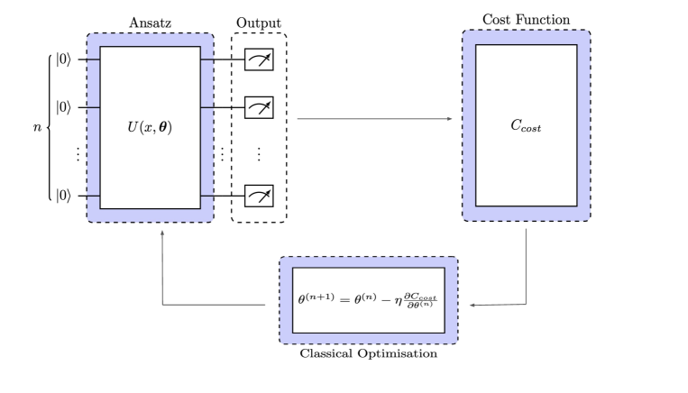
Figure 1: An overview of a variational quantum circuit consisting of its key components - the ansatz, computation of the cost function and updating the parameters via a classical optimisation scheme (with the classical optimiser being gradient descent in this case).

Classical machine learning faces many difficult problems to solve. An empirical approach is what is adopted, relying on benchmarks to assess their performance. However, within deep learning, there is still a lot of work to be done when it comes to the theoretical explanations of such algorithms. In fact, a lot of the problems solved by such algorithms are computationally hard.

This is a problem for both near-term and fault-tolerant quantum machine learning. Noisy Intermediate Scale Quantum (NISQ) computers allow quantum machine learning algorithms to run immediately. But, to perform benchmarks on such hardware and simulators, one has to work under strict design limitations. The algorithms should necessarily have only a few qubits and gates since larger routines run the risk of being a victim of large amounts of noise and, thus, not being simulatable.

To overcome this problem, an idea was to use hybrid quantum-classical algorithms wherein you allow for certain parts of the machine learning pipeline to run on a quantum computer and others to classical computers. One of the ways to divide the work is to have the machine learning model as a quantum algorithm while outsourcing the training aspect to a classical computer. Candidates for such a process are the Variational Circuits (VQCs).

Instead of having a fixed sequence of gates, these algorithms use a template called an Ansatz, which defines a model. These Ansatz can be repeated multiple times in layers. They are called Variational, since they depend on parameters that can be tuned (varied) freely. These parameters are chosen by a classical training scheme, which optimises a cost function specific to the problem. The training usually takes place in a feedback-loop type fashion, similar to classical machine learning training. An overview of a VQC can be seen in Fig. 1 (circuits were made with the help of quantikz [10]). These are, therefore, a family of algorithms, from which an optimal one is chosen following optimisation.

2.1 Interpreting variational quantum circuits as models

In order to interpret a quantum circuit model as a variational quantum circuit, we apply the quantum circuit $U(x,\bm{\theta})$, that depends on both the input $x$ and the parameters $\bm{\theta}$ on the initial state $\ket{0}=\ket{00\cdots 0}$ to get the output $\ket{\psi(x,\bm{\theta})}$. We can then either use the probabilities of the output states $\ket{x}$, or the expectation value of a measurement observable $M$ as the output of the model. Thus, the model is defined as follows:

$$\mathit{f_{\bm{\theta}}(x)}=|\bra{x}\ket{\psi(x,\bm{\theta})}|^{2},$$ (1)

or

$$\mathit{f_{\bm{\theta}}(x)}=\bra{\psi(x,\bm{\theta})}M\ket{\psi(x,\bm{\theta})}.$$ (2)

There are no concrete rules regarding the internal structure of the circuit, and thus, $U(x,\bm{\theta})$ could be anything. It is common to choose one which consists of various layers that depend on the input $x$ [1] [11] [12] [13] [14] [15], which is generally responsible for encoding classical data into a quantum format along with further processing if needed, collectively defined as $S(x)$. Following that, a set of parameterized layers that depend on the parameters $\bm{\theta}$, which can again be collectively defined as W$(\bm{\theta})$. Thus,

$$\mathit{U(x,\bm{\theta})}=\mathit{S(x)}\mathit{W(\bm{\theta})}.$$

On comparing the model’s outputs with the outputs that are required, the parameters of the model can be tuned in order to get the desired result via a training scheme. Since the parameters can be tuned freely, the name variational quantum circuits (VQC) is also used in literature.

2.2 Training Variational Circuits

To train variational circuits is to find a set of optimal parameters $\bm{\theta}$ (where $\bm{\theta}$ is a vector containing $\theta_{1},\theta_{2},\cdots,\theta_{n}$ as its components that minimises a cost function specific to a problem. Consider a cost function $C(\bm{\theta})$, which depends on a model $f$, which in turn depends on parameters $\bm{\theta}$. Using the chain rule, the partial derivative of $C,\partial_{\gamma}C(\bm{\theta})$ with respect to a parameter $\gamma\in\bm{\theta}$ can be written as :

$$\partial_{\gamma}C(\bm{\theta})=\frac{\partial C}{\partial f_{\bm{\theta}}}\frac{\partial f_{\bm{\theta}}}{\partial\gamma},$$ (3)

where $\frac{\partial C}{\partial f_{\bm{\theta}}}$ can be computed classically using the chain rule. The second part of the computation, i.e., $\frac{\partial f_{\bm{\theta}}}{\partial\gamma}$ involves differentiating a result that is obtained from a quantum computer, which also involves parameters that are part of the quantum circuit itself. Ideally, we would like to compute its value on the quantum computer without having to go to a classical computer to do the same. However, doing this is not so straightforward. The following analysis is taken from [1], which provides an excellent account of why it is the case.

Let there be a variational quantum circuit where for simplicity, we assume that it depends only on one parameter $\gamma$, which only affects a single gate $\mathcal{G}(\gamma)$. We will then represent the variational circuit as $\mathcal{VG(\gamma)W}$ and use the expectation value as the output. Then, the output is given by :

$$f_{\gamma} =\bra{0}\mathcal{W}^{{\dagger}}\mathcal{G^{{\dagger}}}(\gamma)\mathcal{V}^{{\dagger}}\mathcal{M}\mathcal{V}\mathcal{G}(\gamma)\mathcal{W}\ket{0},$$

$$=\bra{\psi}\mathcal{G^{{\dagger}}(\gamma)BG(\gamma)}\ket{\psi},$$ (4)

where,

$$\ket{\psi} =W\ket{0}\text{ and }\mathcal{B}=\mathcal{V^{{\dagger}}MV}.$$ (5)

Since the expression for the expectation value is linear, the partial derivative $\partial_{\gamma}f_{\gamma}$ is the sum of the terms :

$$\partial_{\gamma}\bra{\psi}\mathcal{G^{{\dagger}}(\gamma)BG(\gamma)}\ket{\psi}=\bra{\psi}\mathcal{G^{{\dagger}}B(\partial_{\gamma}G(\gamma))}\ket{\psi}+\bra{\psi}\mathcal{(\partial_{\gamma}G^{{\dagger}}\gamma)BG}\ket{\psi}.$$ (6)

Here in Eqn. 6, each term by itself is not an expectation value since the bra and the ket states are not the same. Moreover, we do not know whether the partial derivatives of the gates $\mathcal{G}$ and $\mathcal{G}^{{\dagger}}$, $\partial_{\gamma}G$ or $\partial_{\gamma}G^{{\dagger}}$ are unitary, and hence, do not know whether they can be implemented. It is therefore unclear as to how to execute the calculation of the partial derivative of the quantum computation on a quantum computer directly.

However, it can be shown in certain situations that this partial derivative can be computed by evaluating the expectation values twice by considering different points in the parameter space. This is called the “Parameter Shift Rule”, which is introduced below.

3 The Parameter Shift Rule

We will present here the formulation of this rule chronologically. The first formulation of this was given by Mitrai et al. in their seminal paper titled “Quantum Circuit Learning” [16], after which Schuld et al. [9] expanded on their work. We present the work done by Mitrai et al. first, followed by the work of Schuld et al.

3.1 Formulation of Mitrai et al.

We intend to calculate the derivative of the expectation value of an observable with respect to a circuit parameter $\theta_{j}\in\bm{\theta}$ . In the formulation mentioned here [16], it is supposed for convenience that the unitary $U(\mathbf{\bm{\theta}})$ consists of a chain of unitary transformations $\prod\limits_{j=1}^{k}U_{j}(\theta_{j})$ on a state $\ket{\psi_{in}}$ whose density matrix is given by $\rho_{in}$ and the observable is given by $B$. They also use the notation $U_{j:k}=U_{j}\cdots U_{k}$. Then, $\expectationvalue{B(\mathbf{\bm{\theta}})}$ is given by:

$$\expectationvalue{B(\mathbf{\bm{\theta}})} =\bra{\psi}B\ket{\psi}$$ (7)

$$=\bra{\psi_{in}}U_{l:1}^{{\dagger}}BU_{l:1}\ket{\psi_{in}}$$

$$=\mathrm{Tr}(BU_{l:1}\rho_{in}U_{l:1}^{{\dagger}}).$$

They then make the assumption that the unitaries can be expressed as an exponential with the generator of the unitary being a product of Pauli operators independent of its parameter $\theta_{j}$, i.e., $U_{j}=e^{-\frac{i}{2}\theta_{j}P_{j}}$. Then, on calculating the gradient $\frac{\partial\expectationvalue{B(\mathbf{\theta_{j}})}}{\partial\theta_{j}}$, we get :

$$\frac{\partial\expectationvalue{B(\mathbf{\bm{\theta}})}}{\partial\theta_{j}} =\frac{\partial}{\partial\theta_{j}}(Tr(BU_{l:1}\rho_{in}U_{l:1}^{{\dagger}})),$$

$$=\mathrm{Tr}(B\frac{\partial U_{l:1}}{\partial\theta_{j}}\rho_{in}U_{l:1}^{{\dagger}}+BU_{l:1}\rho_{in}\frac{\partial U_{l:1}^{{\dagger}}}{\partial\theta_{j}}),$$

$$=\mathrm{Tr}(BU_{l:j+1}\frac{\partial U_{j}}{\partial\theta_{j}}U_{j-1:1}\rho_{in}U_{l:1}^{{\dagger}}+BU_{l:1}\rho_{in}U_{j-1:1}^{{\dagger}}\frac{\partial U_{j}^{{\dagger}}}{\partial\theta_{j}}U_{l:j+1}^{{\dagger}}),$$

$$=\mathrm{Tr}(BU_{l:j+1}(-\frac{i}{2}P_{j}U_{j})U_{j-1:1}\rho_{in}U_{l:1}^{{\dagger}}+BU_{l:1}\rho_{in}U_{j-1:1}^{{\dagger}}(\frac{i}{2}P_{j}U_{j}^{{\dagger}})U_{l:j+1}^{{\dagger}}),$$

$$=-\frac{i}{2}\mathrm{Tr}(BU_{l:j+1}P_{j}U_{j:1}\rho_{in}U_{l:1}^{{\dagger}}-BU_{l:1}\rho_{in}U_{j-1:1}^{{\dagger}}P_{j}U_{l:j}^{{\dagger}}),$$

$$=-\frac{i}{2}\mathrm{Tr}(B(U_{l:j}P_{j}U_{j-1:1}\rho_{in}U_{j-1:1}^{{\dagger}}U_{l:j}^{{\dagger}}-U_{l:j}U_{j-1:1}\rho_{in}U_{j-1:1}^{{\dagger}}P_{j}U_{l:j}^{{\dagger}})),$$

$$=-\frac{i}{2}\mathrm{Tr}(BU_{l:j}(P_{j}U_{j-1:1}\rho_{in}U_{j-1:1}^{{\dagger}}-U_{j-1:1}\rho_{in}U_{j-1:1}^{{\dagger}}P_{j})U_{l:j}^{{\dagger}})),$$

$$=-\frac{i}{2}\mathrm{Tr}(BU_{l:j}\big{[}P_{j},U_{j-1:1}\rho_{in}U_{j-1:1}^{{\dagger}}\big{]}U_{l:j}^{{\dagger}})).$$

On using the following property of the commutator:

$$\big{[}P_{i},\rho\big{]}=i\bigg{[}U_{j}\bigg{(}\frac{\pi}{2}\bigg{)}\rho U_{j}^{{\dagger}}\bigg{(}\frac{\pi}{2}\bigg{)}-U_{j}\bigg{(}-\frac{\pi}{2}\bigg{)}\rho U_{j}^{{\dagger}}\bigg{(}-\frac{\pi}{2}\bigg{)}\bigg{]},$$ (8)

we get the gradient to be :

$$\frac{\partial\expectationvalue{B(\mathbf{\bm{\theta}})}}{\partial\theta_{j}}= \frac{1}{2}\mathrm{Tr}\bigg{[}BU_{l:j}U_{j}\bigg{(}\frac{\pi}{2}\bigg{)}\rho_{j}U_{j}^{{\dagger}}\bigg{(}\frac{\pi}{2}\bigg{)}U_{l:j}^{{\dagger}}\bigg{]}$$ (9)

$$-\frac{1}{2}\mathrm{Tr}\bigg{[}BU_{l:j}U_{j}\bigg{(}-\frac{\pi}{2}\bigg{)}\rho_{j}U_{j}^{{\dagger}}\bigg{(}-\frac{\pi}{2}\bigg{)}U_{l:j}^{{\dagger}}\bigg{]},$$

where $\rho_{j}=U_{j:1}\rho_{in}U_{j:1}^{{\dagger}}$. Thus, by just inserting a $\pm\big{(}\frac{\pi}{2}\big{)}$ as a parameter for an extra gate in front of the gate whose gradient we would like to calculate and measure the resulting expectation values $\expectationvalue{B}_{j}^{\pm}$, we can calculate the exact analytical gradient of the observable $\expectationvalue{B}$ using $\frac{\expectationvalue{B}^{+}-\expectationvalue{B}^{-}}{2}$.

3.2 Formulation of Schuld et al.

While the above formulation assumed the existence of an expression for a gate as an exponential of a Pauli product independent of its parameters, this work [9] aims to further expand on the idea. Here, it is shown that any gate of the form $U_{j}=e^{-i\theta_{j}\mathcal{G}}$ where $\mathcal{G}$ is a Hermitian with at most two distinct eigenvalues obeys the parameter shift rule for calculating its derivative. Let the overall unitary be $U(\mathbf{\bm{\theta}})$, which can be decomposed into several single-parameter gates. For simplicity, we assume that parameter $\theta_{j}\in\mathbf{\bm{\theta}}$ only affects a single gate $U_{j}(\theta_{j})$ in the sequence $U(\mathbf{\bm{\theta}})=VU_{j}(\theta_{j})W$. The partial derivative is then given by :

$$\partial_{\theta_{j}}f =\partial_{\theta_{j}}\bra{0}U(\mathbf{\bm{\theta}})^{{\dagger}}BU(\mathbf{\bm{\theta}})\ket{0}$$ (10)

$$=\partial_{\theta_{j}}\bra{0}(VU_{j}(\theta_{j})W)^{{\dagger}}BVU_{j}(\theta_{j})W\ket{0}$$

$$=\partial_{\theta_{j}}\bra{0}W^{{\dagger}}U_{j}(\theta_{j})^{{\dagger}}V^{{\dagger}}BVU_{j}(\theta_{j})W\ket{0}$$

$$=\partial_{\theta_{j}}\bra{\psi}U_{j}^{{\dagger}}QU_{j}\ket{\psi}$$

$$=\bra{\psi}U_{j}^{{\dagger}}Q(\partial_{\theta_{j}}U_{j})\ket{\psi}+\bra{\psi}(\partial_{\theta_{j}}U_{j}^{{\dagger}})QU_{j}\ket{\psi},$$

where $Q=V^{{\dagger}}BV$ and $\ket{\psi}=W\ket{0}$.

Now, for any two operators $A,B$ we have:

$$\bra{\psi}A^{{\dagger}}QB\ket{\psi}+h.c.= \frac{1}{2}\big{(}\bra{\psi}(A+B)^{{\dagger}}Q(A+B)\ket{\psi}-\bra{\psi}(A-B)^{{\dagger}}Q(A-B)\ket{\psi}\big{)}.$$ (11)

Hence, in order to implement Eqn. 10, we can use the above expression. If we are able to implement $(U_{j}\pm\partial_{\theta_{j}}U_{j})$ as a unitary gate itself, we can directly evaluate Eqn. 10 on the quantum computer itself, since the two terms that are subtracted in the Eqn. 11 represent expectation values with respect to the observable $Q$ and states $(A\pm B)\ket{\psi}$. What remains is to check whether $(A\pm B)$ is unitary, which here, translates to establishing which gates obey the condition of $U_{j}\pm\partial_{\theta_{j}}U_{j}$ being unitary.

Consider a gate $U_{j}=e^{-i\theta_{j}\mathcal{G}}$ where $\mathcal{G}$ is a Hermitian with at most two distinct eigenvalues. Its derivative comes out to be:

$$\partial_{\theta_{j}}U_{j}(\theta_{j})=-i\mathcal{G}e^{-i\theta_{j}\mathcal{G}}.$$ (12)

On substituting Eqn. 12 into Eqn. 10, we get:

$$\partial_{\theta_{j}}f=\bra{\psi\prime}Q(-i\mathcal{G})\ket{\psi\prime}+\bra{\psi\prime}(i\mathcal{G})Q\ket{\psi\prime},$$ (13)

where $\ket{\psi^{{}^{\prime}}}=\mathcal{G}\ket{\psi}$. If $\mathcal{G}$ has only two distinct eigenvalues (which can be repeated) [9], without loss of generality, we can shift the eigenvalues to $\pm r$, as the global phase remains unobservable. It should be noted that every single qubit gate is of this form. Thus, we can write:

$$\partial_{\theta_{j}}f=r(\bra{\psi\prime}\mathds{1}Q(-ir^{-1}\mathcal{G})\ket{\psi\prime}+\bra{\psi\prime}(ir^{-1}\mathcal{G})Q\mathds{1}\ket{\psi\prime}).$$ (14)

On applying Eqn. 11 to the above expression (Eqn. 14), we get:

$$\partial_{\theta_{j}}f= \frac{r}{2}\big{(}\bra{\psi\prime}(\mathds{1}-ir^{-1}\mathcal{G})^{{\dagger}}Q(\mathds{1}-ir^{-1}\mathcal{G})\ket{\psi\prime}$$ (15)

$$-\bra{\psi\prime}(\mathds{1}+ir^{-1}\mathcal{G})^{{\dagger}}Q(\mathds{1}+ir^{-1}\mathcal{G})\ket{\psi\prime}\big{)}.$$

Thus, if we can show that in Eqn. 15, $(\mathds{1}\mp ir^{-1}\mathcal{G})$ is unitary, we can evaluate the gradient directly on a quantum computer. We now show that $(\mathds{1}\mp ir^{-1}\mathcal{G})$ is unitary, and in fact, there exist values for $\theta_{j}$ for which $U_{j}(\theta_{j})$ becomes $\frac{1}{\sqrt{2}}(\mathds{1}\pm ir^{-1}\mathcal{G})$.

Theorem. If the Hermitian generator $\mathcal{G}$ of the unitary operator $U_{j}(\theta_{j})=e^{-i\theta_{j}\mathcal{G}}$ has at most two unique eigenvalues $\pm r$, then the following identity holds:

$$\mathcal{G}\bigg{(}\frac{\pi}{4r}\bigg{)}=\frac{1}{\sqrt{2}}(\mathds{1}\pm ir^{-1}\mathcal{G})$$ (16)

Proof : Since $\mathcal{G}$ has a spectrum $\{\pm r\}$, it implies that $\mathcal{G}^{2}=r^{2}\mathds{1}$. Keeping that in mind, the Taylor Series expansion of $U_{j}(\theta_{j})$ is given by:

$$U_{j}(\theta_{j}) =e^{-i\theta_{j}\mathcal{G}}=\sum_{k=0}^{\infty}\frac{(-i\theta_{j})^{k}\mathcal{G}^{k}}{k!}$$ (17)

$$=\sum_{k=0}^{\infty}\frac{(-i\theta_{j})^{2k}\mathcal{G}^{2k}}{(2k)!}+\sum_{k=0}^{\infty}\frac{(-i\theta_{j})^{2k+1}\mathcal{G}^{2k+1}}{(2k+1)!}$$

$$=\mathds{1}\sum_{k=0}^{\infty}\frac{(-1)^{k}(r\theta_{j})^{2k}}{(2k)!}-ir^{-1}\mathcal{G}\sum_{k=0}^{\infty}\frac{(-1)^{k}(r\theta_{j})^{2k+1}}{(2k+1)!}$$

$$=\mathds{1}\cos{(r\theta_{j})}-ir^{-1}\mathcal{G}\sin{(r\theta_{j})}.$$

Hence, we get $\mathcal{G}\big{(}\frac{\pi}{4r}\big{)}=\frac{1}{\sqrt{2}}(\mathds{1}\pm ir^{-1}\mathcal{G})$.

Thus, if the Hermitian generator of the unitary operator to be differentiated has at most two unique eigenvalues, $\partial_{\theta_{j}}f$ can be evaluated using two extra evaluations of expectation values on the quantum device, with each having the gate $\mathcal{G}\big{(}\pm\frac{\pi}{4r}\big{)}$ placed in front of the gate to be differentiated. Since $\mathcal{G}(a)\mathcal{G}(b)=\mathcal{G}(a+b)$ for single parameter gates, what we have arrived at is the equivalent of shifting the gate parameter of the gate to be differentiated by $s=\frac{\pi}{4r}$, which is termed as the “parameter shift rule”.

$$\partial_{\theta_{j}}f =r\big{(}\bra{\psi}\mathcal{G}^{{\dagger}}(\theta_{j}+s)Q\mathcal{G}(\theta_{j}+s)\ket{\psi}$$ (18)

$$-\ \bra{\psi}\mathcal{G}^{{\dagger}}(\theta_{j}-s)Q\mathcal{G}(\theta_{j}-s)\ket{\psi}\big{)},$$

$$=r\big{(}f(\theta_{j}+s)-f(\theta_{j}-s)\big{)}.$$

In the case of $\theta_{j}$ appearing in more than one gate in a single circuit, the derivative can be obtained by using the product rule by shifting the parameter in each gate separately and summing up the results. It can be seen that Eqn. 18 looks like the finite differences method, except for having a macroscopic shift and the value is exact.

4 Choice of ansatz and cost function for optimisation

In order to come up with an ansatz (or the model, as described in Sec. 2.2) for a problem, as mentioned before, there are no rules/guidelines. They are very problem-specific and context-dependent. However, there may be a few things that can help while coming up with one. Its structure can be influenced with respect to some aspects of the underlying physics, chemistry or quantum information theory. It might also have to do with the problem’s underlying structure or an intuition borrowed from machine learning. However, ansatz may, in fact, have no basis at all and happens to work.

For generating probability distributions, in [4], a general framework was given as to which circuit architecture works well for generating which type of distribution. In the paper, they broadly categorise them into circuits for generating symmetric distributions and asymmetric distributions. Corresponding to each of the two cases, a constraint is derived for the parameterized gates, which were then used to optimise the circuit using the COBYLA optimiser. However, instead of doing that, we look at several kinds of variational circuit architectures, each corresponding to the number of qubits. We then run them and check to see which one does best.

The ansatze that were tested for the problem of focus in this work are presented in Fig. 2, Fig. 3, Fig. 4 (circuit diagrams were made using quantikz [10]). The four qubit ansatze’ structure was influenced by [17]. In [17], a case was made to study the expressibility of each of the circuits. The circuits studied by them are used as ansatze for our purposes here. Here, the three and two qubit structures were made similar to the four qubit ones.

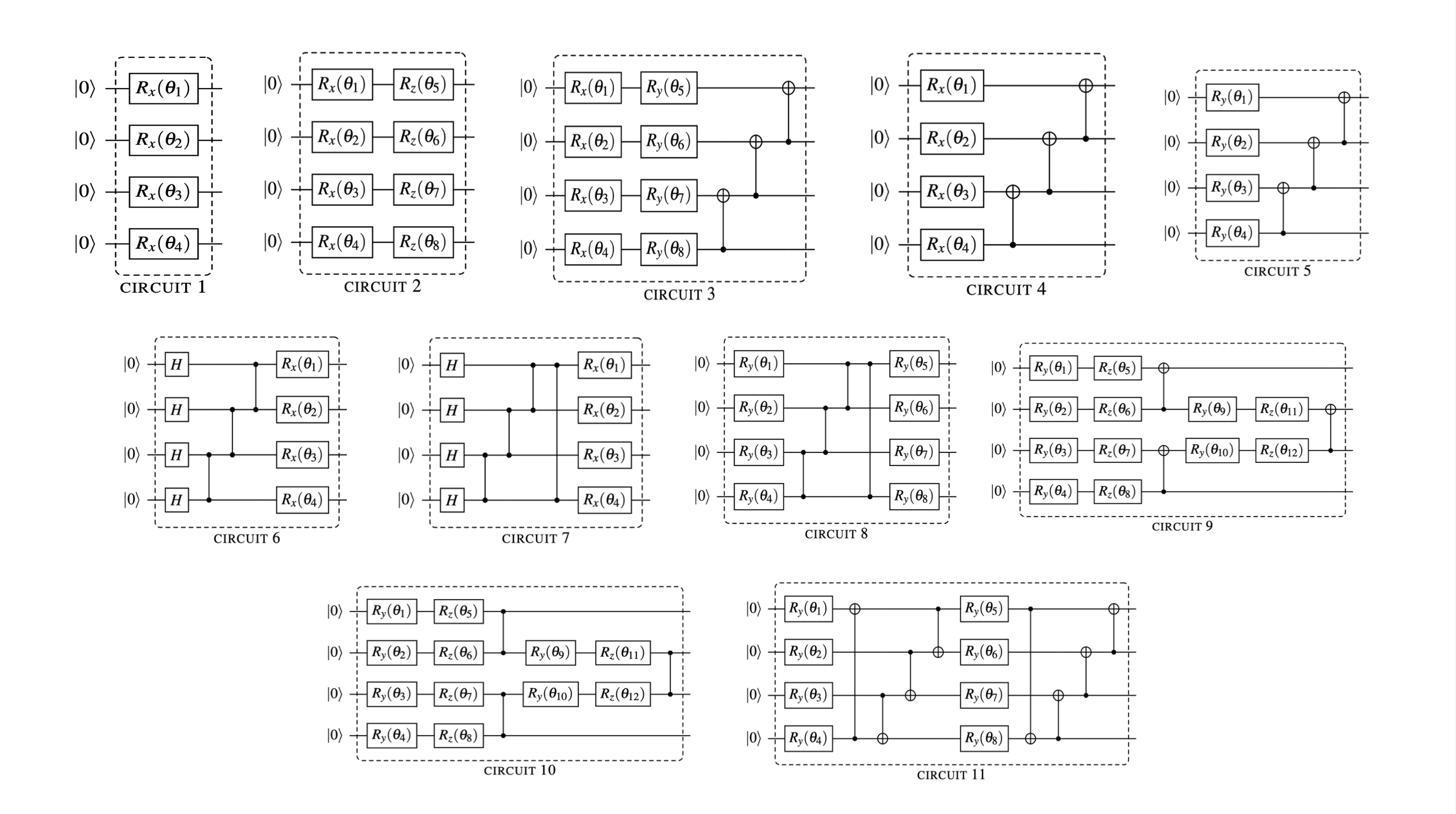
Figure 2: Four qubit ansatze (circuits-2, 3, 6, 8, 9, and 11 are from [17]) consisting of parameterized layers, entangling layers for generating Uniform, Normal, Binomial and Poisson distributions.

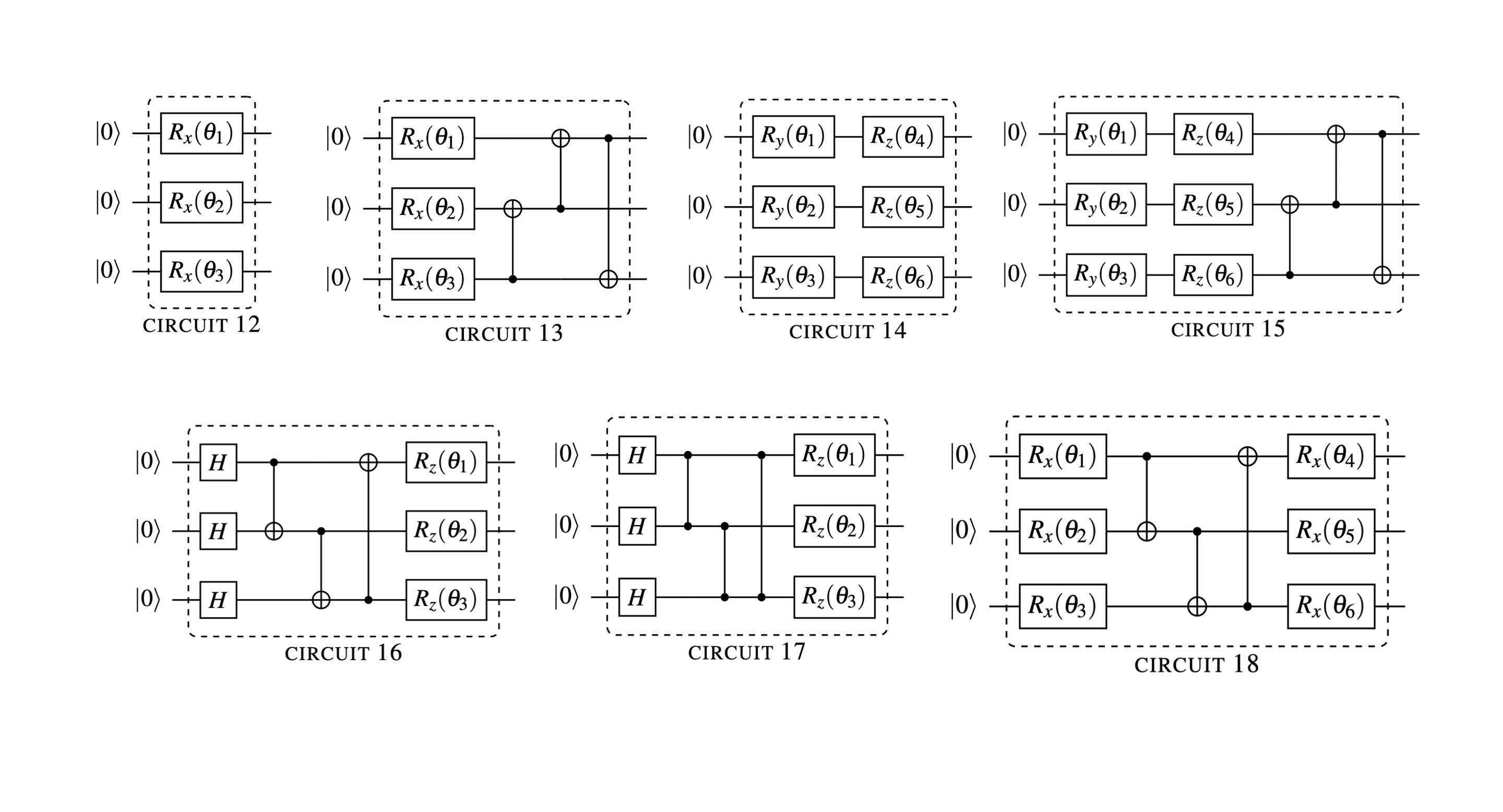
Figure 3: Three qubit ansatze consisting of parameterized layers, entangling layers for generating Uniform, Normal, Binomial and Poisson distributions.

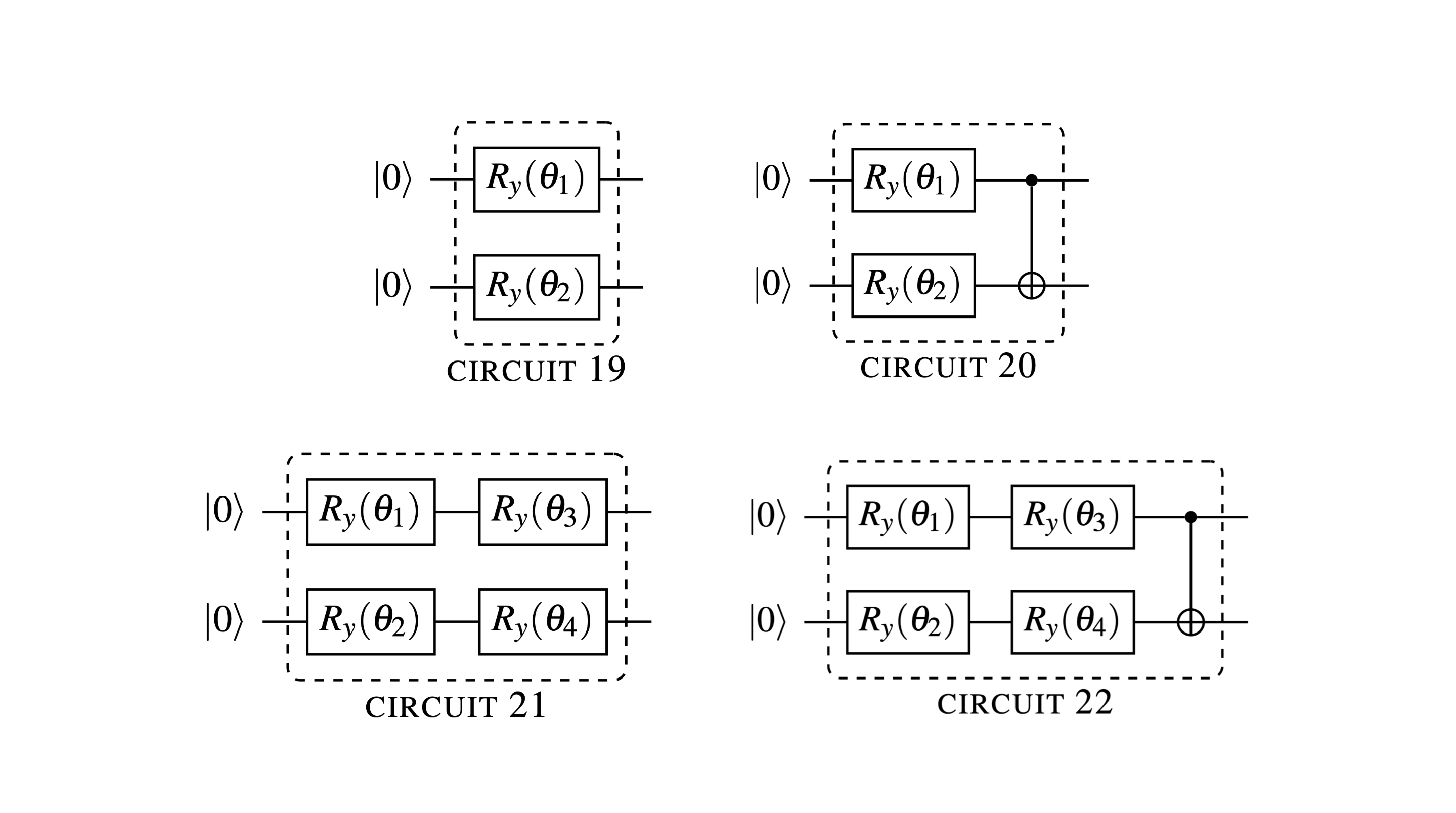
Figure 4: Two qubit ansatze consisting of parameterized layers, entangling layers for generating Uniform, Normal, Binomial and Poisson distributions.

4.1 Optimisation

We use Pennylane for our simulations. In order to run a circuit in Pennylane, one needs to define the circuit (which is done as a python function - the quantum function), and define a computational device (quantum device) on which the circuit is to be run. The device can either be a simulator or a real hardware. The quantum device and the function together are used to create a quantum node, which binds the function to the device. For our study, we have used the ‘default.qubit’ device (which is a circuit simulator). On running the ansatz, the probabilities can be obtained using the ‘qml.probs()’ argument, which returns an array consisting of the probabilities of the computational basis states in lexicographic order. Fig. 5 shows an example of a histogram of the probabilities of output states for a two qubit system.

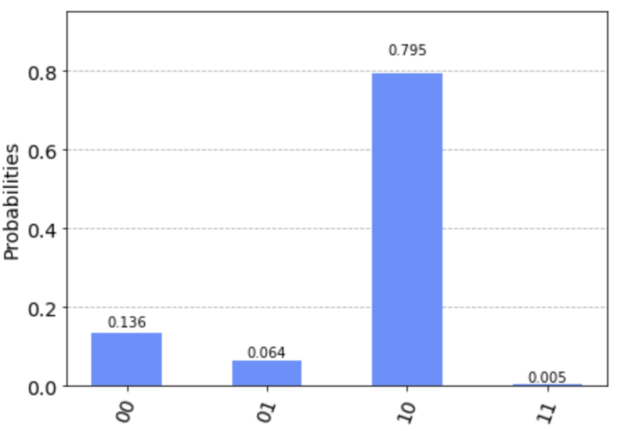
Figure 5: An example of a probability distribution as generated by a two- qubit circuit.

Then, to understand how well the model has performed, we compare the output with the desired probability distribution and calculate the cost using the cost function or the loss function. This cost serves as the benchmark to see whether the next round of training is better or worse than the previous round.

The gradient descent is a popular method for optimisation. Here, the parameters are updated in such a manner so as to decrease the cost value via going down the cost landscape [18]. This is done by virtue of taking the gradient as can be seen in its expression:

$$\theta^{(n+1)}=\theta^{(n)}-\eta\frac{\partial C}{\partial\theta^{(n)}},$$ (19)

where, $\theta^{(n)}$ is value of the parameter $\theta$ at the $n$th iteration, and $\eta$ is the learning rate.

The basic requirement of the method is the availability of gradients, which, as shown in Sec. 2.2, is not straightforward to calculate on a quantum computer [1]. In order to calculate the gradients, we shall use the parameter shift rule introduced in Sec. 3 [16] [9]. However, for our purposes, we shall use the probability values of the output states as the output rather than the expectation values. The parameter shift rule still holds valid, since the probability values are also a kind of expectation value [1]. Nevertheless, the proof is given in the appendix section (Section A), which follows the same outline as that presented in [16].

4.2 Cost functions and target distributions

Cost functions such as the Least Squares Error, the Kullback-Leibler (KL) Divergence and the Jensen-Shannon (JS) Divergence are commonly used for various machine learning tasks. The Least Squares Error is a basic cost function used in regression analyses and data fitting, while the other two are measures of information [19]. Their expressions are as follows:

$$C_{\textit{LSE}} =\sum_{x=1}^{2^{n}}(P(x)-Q(x))^{2}$$ (20)

$$C_{\textit{KL}} =\sum_{x=1}^{2^{n}}P(x)\log{\bigg{(}\frac{P(x)}{Q(x)}\bigg{)}}$$ (21)

$$C_{\textit{JS}} =\sum_{x=1}^{2^{n}}P(x)\log{\bigg{(}\frac{P(x)}{\frac{P(x)+Q(x)}{2}}\bigg{)}}+\sum_{x=1}^{2^{n}}Q(x)\log{\bigg{(}\frac{Q(x)}{\frac{P(x)+Q(x)}{2}}\bigg{)}}$$ (22)

where $n$ is the number of qubits, $P(x)$ is the output probability distribution (from the model) and $Q(x)$ is the desired probability distribution.

In order to compare two probability distributions, $P(x)$ and $Q(x)$, over the same random variable $x$, the KL Divergence is a good measure. It has many useful properties, the most notable being that it is non-negative. The KL divergence is $0$ only when the two distributions $P$ and $Q$ are the same. The KL divergence is thus, a good indicator of the similarity between two probability distributions. However, this function is not symmetric, i.e., $C_{KL}(P||Q)\neq C_{KL}(Q||P)$, for some $P$ and $Q$. Thus, it is non-trivial as to whether one should use $C_{KL}(P||Q)$ or $C_{KL}(Q||P)$ [18]. In order to avoid this problem, we primarily use only one cost function to quantify the error - the JS Divergence, which is a symmetric form of the KL divergence [19]. As far as the Least Squares Error is concerned, it does a terrible job in comparing two probability distributions.

The probability distributions to be generated in this study are the Uniform, Normal, Binomial and Poisson distributions. They are defined below.

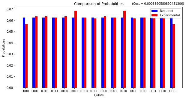
Figure 6: Uniform Distribution as simulated by the four qubit ansatz (circuit-8).

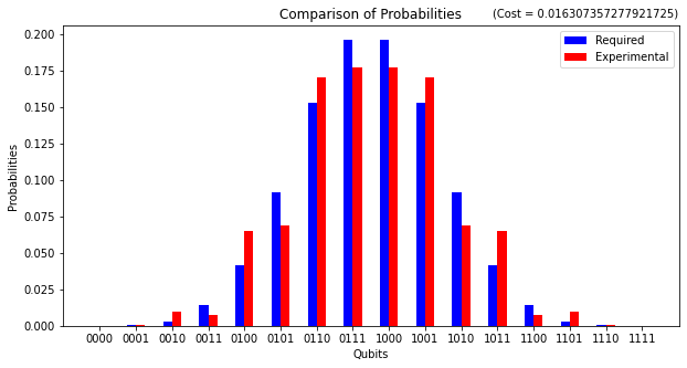
Figure 7: Normal Distribution as simulated by the four qubit ansatz (circuit-8).

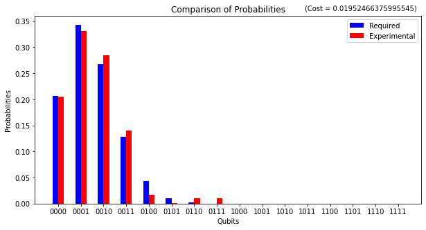
Figure 8: Binomial Distribution as simulated by the four qubit ansatz (circuit-8).

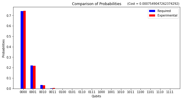
Figure 9: Poisson Distribution as simulated by the four qubit ansatz (circuit-8).

A Normal distribution is a probability distribution where a continuous random variable $X$ follows a probability density defined by :

$$P(x)=\frac{1}{\sqrt{2\pi}}e^{\frac{-x^{2}}{2}},$$

where $x\in X$.

A Binomial distribution is a probability distribution where the random variable $X$ takes values $0,1,2,...,N$ with probabilities :

$$P(X=k)=\begin{pmatrix}n\\ k\end{pmatrix}p^{k}(1-p)^{(n-k)},$$

where $0<p<1$. The binomial distribution chosen for the purpose of this study takes $p$ to have the value $0.1$. Also, since the normal distribution is a continuous distribution, in order to discretize it, we have used a binomial distribution with p = 0.5 as the normal distribution.

A Poisson distribution is a probability distribution where the discrete random variable $X$ has the probability mass function given by :

$$P(X=k)=\frac{\lambda^{k}e^{-\lambda}}{k!},$$

where $\lambda>0$.

The gradient descent optimiser is thus used, taking the JS divergence as our cost function. The gradient descent optimiser is available for use in Pennylane as ‘qml.GradientDescentOptimiser()’. The differentiation method is chosen to be parameter shift by specifying diff_method = "parameter-shift" in the qnode decorator, and the stepsize for the gradient descent is taken to be 0.1, while running it for 1000 iterations. As an example, we show the outputs simulated by circuit 8 in Fig. 6, Fig. 7, Fig. 8 and Fig. 9 for the Uniform, Normal, Binomial and Poisson distributions, respectively.

5 Simulation results and discussion

We simulate all 22 circuit ansatze. The results for the four qubit, three qubit and two qubit simulations are shown in Fig. 10, Fig. 11 and Fig. 12, respectively.

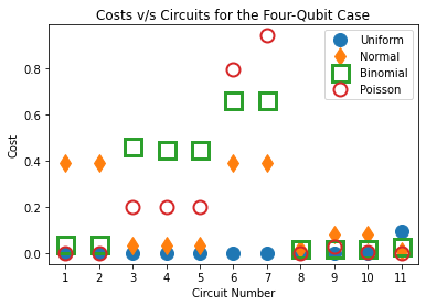
Figure 10: Accuracy of the generated probability distributions as quantified by the JS Divergence for the four qubit ansatze.

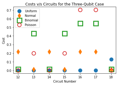
Figure 11: Accuracy of the generated probability distributions as quantified by the JS Divergence for the three qubit ansatze.

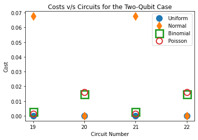
Figure 12: Accuracy of the generated probability distributions as quantified by the JS Divergence for the two qubit ansatze.

When it comes to the uniform distribution, we observe that all the circuits seem to generate it really well. This may be because the initial state already represents a uniform distribution and, thus, can be replicated easily. While this hypothesis can be tested using an initial state that represents a certain distribution, say normal, and running the same procedure with this initial state and looking at the ease of reproducing normal distributions, it would beat the purpose of generating such states in the first place. This is also a trivial use-case of the algorithm since most circuits start off with a uniform distribution of the ground state. Regarding the binomial, however, a pattern can be seen in normal and Poisson distributions.

In the four qubit case, particularly focusing on circuits - 1 through 5, we see that circuit - 1 and circuit - 2 reproduce the Binomial and Poisson distributions well while being unable to produce the Normal distribution. However, we observe the opposite pattern in circuits 3, 4, and 5. They generate the normal distribution well while being unable to generate the Binomial and Poisson distributions nicely. From this, a conclusion can be drawn about generating said distributions, that is, an ansatz only having a parameterized layer (a layer containing gates that are parameterized) is not able to generate Normal distributions while doing well in Binomial and Poisson distributions; and an ansatz only having a parameterized layer followed by an entangling layer (a layer consisting of entangling gates) does well in generating Normal distributions, but does not do well in generating Binomial and Poisson distributions. We also observe that the type of parameterized gate ($R_{x}$ or $R_{y}$, for example) does not matter in their reproduction, as is observed by the fact that both circuit - 4 and circuit - 5 do well in reproducing the normal distribution. It can also be seen that out of all the four qubit circuits, circuits - 8 through 11 work the best. This makes sense since the extra parameterized layer that follows the parameterized and entangling layer helps in balancing out what just the parameterized layer or just the parameterized and entangling layer could not achieve on their own (as seen in circuits 1 through 5). As far as circuits - 6 and 7 go, they do not generate any of the said distributions well. It is hypothesised here that having the state beginning from a uniform superposition does not allow for the preparation of said probability distributions.

In the three-qubit case, circuits - 12 and 14 do well in generating the Binomial and Poisson distributions while not doing well in generating the Normal distribution. Circuits - 13 and 15 do the opposite, wherein they do well in generating the Normal distribution but not the Binomial and Poisson distributions. This is in line with the hypothesis presented in the four qubit case, where it was noted that having only a parameterised layer is not capable of generating Normal distributions, and only having a parameterised layer followed by an entangling layer is not capable of generating Binomial and Poisson distributions well. Having an extra parameterized layer that follows the parameterized and entangling layers also helps in this situation, as is observed by the good performance of circuit - 18 on generating all distributions. Circuits - 16 and 17 do not do well in generating the distributions, and this is in accordance with the hypothesis presented for circuits - 6 and 7, i.e., an initial uniform superposition does not allow for the preparation of said distributions. The poor performance, in this case, can also be attributed to the fact that these circuits consist of RZ gates, which do not have any impact on the training since a rotation about the Z axis would not provide any measurable difference in the probabilities of the basis states as measured in the computational basis.

In the two-qubit case, the same relative pattern of only parameterized layers doing well in generating the Binomial and Poisson distributions while having a parameterized layer followed by an entangling layer doing well in Normal distributions is observed. However, in absolute terms, all the two-qubit ansatze do well in generating said distributions.

6 Conclusion

We present a variational method to generate probability distributions using quantum circuits. The probability distributions generated here include the Uniform, Normal, Binomial and Poisson distributions. The error is quantified using the JS Divergence as the cost function, while the parameters are optimised using gradient descent and the parameter shift rule to calculate the gradients. The simulations are done using Pennylane as the software framework.

It is initially observed for certain distributions, and certain architectures do better than others. This architecture remains constant across the number of qubits. For generating normal distributions, the best architecture is seen to consist of a parameterized layer (a layer containing only parameterized gates) followed by an entangling layer (a layer containing only entangling gates). For generating Binomial and Poisson distributions, the best architecture is seen to consist of having just a parameterized layer. As far as Uniform distributions go, all the circuits do well in generating them. Bearing this in mind, having a parameterized layer (that does well in generating Binomial and Poisson distributions) that follows a parameterized layer and an entangling layer (that does well in generating Normal distributions) is seen to do well in generating all distributions. This is believed to be so because in this case, the layers balance out the flaws in the above two cases to be able to generate all the distributions well.

It is also noticed that having RZ gates as part of the parameterized layers generally does not do much since their action on the qubit does not translate to a difference in the observed probabilities of the basis state measured in the computational basis. Insofar as the type of parameterized gates required for the parameterized layer, no change in accuracy is observed by either the type of gate (RX or RY), or the number of times it is repeated on the same qubit within the same layer. Having the initial state initialised to a uniform superposition renders the circuit incapable of generating any of the distributions (except Uniform) well. Thus, in order to generate all the distributions (Uniform, Normal, Binomial and Poisson) well (as quantified by the JS divergence), the optimal circuit ansatz is seen to be a parameterized layer consisting of single qubit rotation gates (either RX or RY) on each qubit, followed by an entangling layer, followed by another parameterized layer consisting of single qubit rotation gates (either RX or RY) on each qubit.

With this being said, however, giving any concrete rules regarding which architectures suit which distributions and what makes an ansatz “better” requires a lot more study. Instead of looking at this study as a concrete definition of any rules that govern a “best” ansatz, it should be viewed as a technique to generate probability distributions that give rise to certain patterns regarding the ansatz that provide optimal use-case in this context. Further work on this study is required to test the claims with a larger sample space of circuits. A few things that can be tested are whether repeating these circuits as templates helps in reproducing the distributions better, what kind of entangling layers have what kind of effect in generating distributions and different measures of accuracy to judge which circuits accurately generate probability distributions.

Appendix A Parameter-Shift rule for probabilities of states as output

Let there be a quantum circuit with unitary $W(\mathbf{\theta})$, which consists of a chain of unitary transformations $\prod\limits_{j=1}^{k}U_{j}(\theta_{j})$ on a state $\psi_{in}$ whose density matrix is given by $\rho_{in}$. Then, with :

$$\ket{\psi}=W\ket{\psi_{in}},$$ (23)

the output reads:

$$f_{\theta_{j}} =\absolutevalue{\innerproduct{x_{i}}{\psi}}^{2},$$ (24)

$$=\absolutevalue{\bra{x_{i}}W\ket{\psi_{in}}\bra{\psi_{in}}W^{{\dagger}}\ket{x_{i}}},$$

$$=\mathrm{Tr}(W\rho_{in}W^{{\dagger}}X),$$

where, $X=\ket{x_{i}}\bra{x_{i}}$.

We use the notation $U_{j:k}=U_{j}...U_{k}$ for convenience. Therefore, from Eqn. 24, we have :

$$\frac{\partial p\big{(}\ket{x_{i}}\big{)}}{\partial\theta_{j}} =\frac{\partial\text{Tr}(W\rho W^{{\dagger}}X)}{\partial\theta_{j}}$$

$$=\text{Tr}\bigg{(}(\partial_{\theta_{j}}W)\rho W^{{\dagger}}X\bigg{)}+\text{Tr}\bigg{(}W\rho(\partial_{\theta_{j}}W^{{\dagger}})X\bigg{)}$$

$$=\text{Tr}\bigg{(}X(\partial_{\theta_{j}}W)\rho W^{{\dagger}}\bigg{)}+\text{Tr}\bigg{(}XW\rho(\partial_{\theta_{j}}W^{{\dagger}})\bigg{)}$$

$$=\text{Tr}\bigg{(}X(\partial_{\theta_{j}}W)\rho W^{{\dagger}}+XW\rho(\partial_{\theta_{j}}W^{{\dagger}})\bigg{)}$$

$$=\text{Tr}\bigg{(}XU_{n:j+1}\frac{\partial U_{j}}{\partial\theta_{j}}U_{j-1:1}\rho W^{{\dagger}}+XW\rho U_{j-1:1}^{{\dagger}}\frac{\partial U_{j}^{{\dagger}}}{\partial\theta_{j}}U_{n:j+1}^{{\dagger}}\bigg{)}$$

$$=\text{Tr}\bigg{(}XU_{n:j+1}(-\frac{i}{2}P_{j}U_{j})U_{j-1:1}\rho W^{{\dagger}}+XW\rho U_{j-1:1}^{{\dagger}}(\frac{i}{2}P_{j}U_{j}^{{\dagger}})U_{n:j+1}^{{\dagger}}\bigg{)}$$

$$=\text{Tr}\bigg{(}-\frac{i}{2}X\bigg{(}U_{n:j+1}P_{j}U_{j}U_{j-1:1}\rho W^{{\dagger}}-W\rho U_{j-1:1}^{{\dagger}}P_{j}U_{j}^{{\dagger}}U_{n:j+1}^{{\dagger}}\bigg{)}\bigg{)}$$

$$=\text{Tr}\bigg{(}-\frac{i}{2}X\bigg{(}U_{n:j+1}P_{j}U_{j}U_{j-1:1}\rho W^{{\dagger}}-W\rho U_{j-1:1}^{{\dagger}}U_{j}^{{\dagger}}P_{j}U_{n:j+1}^{{\dagger}}\bigg{)}\bigg{)}$$

$$=\text{Tr}\bigg{(}-\frac{i}{2}X\bigg{(}U_{n:j+1}P_{j}U_{j:1}\rho W^{{\dagger}}-W\rho U_{j:1}^{{\dagger}}P_{j}U_{n:j+1}^{{\dagger}}\bigg{)}\bigg{)}$$

$$=\text{Tr}\bigg{(}-\frac{i}{2}X\bigg{(}U_{n:j+1}P_{j}U_{j:1}\rho U_{j:1}^{{\dagger}}U_{n:j+1}^{{\dagger}}-U_{n:j+1}U_{j:1}\rho U_{j:1}^{{\dagger}}P_{j}U_{n:j+1}^{{\dagger}}\bigg{)}\bigg{)}$$

$$=\text{Tr}\bigg{(}-\frac{i}{2}X\bigg{(}U_{n:j+1}\bigg{(}P_{j}U_{j:1}\rho U_{j:1}^{{\dagger}}-U_{j:1}\rho U_{j:1}^{{\dagger}}P_{j}\bigg{)}U_{n:j+1}^{{\dagger}}\bigg{)}\bigg{)}$$

$$\frac{\partial p\big{(}\ket{x_{i}}\big{)}}{\partial\theta_{j}} =\text{Tr}\bigg{(}-\frac{i}{2}X\bigg{(}U_{n:j+1}\bigg{[}P_{j},U_{j:1}\rho U_{j:1}^{{\dagger}}\bigg{]}U_{n:j+1}^{{\dagger}}\bigg{)}\bigg{)}.$$

Then, on using the following property of the commutator introduced in [16]

$$\big{[}P_{i},\rho\big{]}=i\bigg{[}U_{j}\bigg{(}\frac{\pi}{2}\bigg{)}\rho U_{j}^{{\dagger}}\bigg{(}\frac{\pi}{2}\bigg{)}-U_{j}\bigg{(}-\frac{\pi}{2}\bigg{)}\rho U_{j}^{{\dagger}}\bigg{(}-\frac{\pi}{2}\bigg{)}\bigg{]},$$

we get the following:

$$\frac{\partial p\big{(}\ket{x_{i}}\big{)}}{\partial\theta_{j}}= \frac{1}{2}\mathrm{Tr}\bigg{[}XU_{n:j+1}U_{j}\bigg{(}\frac{\pi}{2}\bigg{)}\rho_{j}U_{j}^{{\dagger}}\bigg{(}\frac{\pi}{2}\bigg{)}U_{n:j+1}^{{\dagger}}-XU_{n:j}U_{j}\bigg{(}-\frac{\pi}{2}\bigg{)}\rho_{j}U_{j}^{{\dagger}}\bigg{(}-\frac{\pi}{2}\bigg{)}U_{n:j+1}^{{\dagger}}\bigg{]}$$

$$= \frac{1}{2}\mathrm{Tr}\bigg{[}XU_{n:j+1}U_{j}\bigg{(}\frac{\pi}{2}\bigg{)}U_{j:1}\rho U_{j:1}^{{\dagger}}U_{j}^{{\dagger}}\bigg{(}\frac{\pi}{2}\bigg{)}U_{n:j+1}^{{\dagger}}$$

$$-\;XU_{n:j+1}U_{j}\bigg{(}-\frac{\pi}{2}\bigg{)}U_{j:1}\rho U_{j:1}^{{\dagger}}U_{j}^{{\dagger}}\bigg{(}-\frac{\pi}{2}\bigg{)}U_{n:j+1}^{{\dagger}}\bigg{]}$$

$$= \frac{1}{2}\mathrm{Tr}\bigg{[}XU_{n:j+1}U_{j}\bigg{(}\theta_{j}+\frac{\pi}{2}\bigg{)}U_{j-1:1}\rho U_{j-1:1}^{{\dagger}}U_{j}^{{\dagger}}\bigg{(}\theta_{j}+\frac{\pi}{2}\bigg{)}U_{n:j+1}^{{\dagger}}$$

$$-\;XU_{n:j+1}U_{j}\bigg{(}\theta_{j}-\frac{\pi}{2}\bigg{)}U_{j-1:1}\rho U_{j-1:1}^{{\dagger}}U_{j}^{{\dagger}}\bigg{(}\theta_{j}-\frac{\pi}{2}\bigg{)}U_{n:j+1}^{{\dagger}}\bigg{]}$$

$$= \frac{1}{2}\mathrm{Tr}\bigg{[}XU_{n:j+1}U_{j}\bigg{(}\theta_{j}+\frac{\pi}{2}\bigg{)}U_{j-1:1}\rho U_{j-1:1}^{{\dagger}}U_{j}^{{\dagger}}\bigg{(}\theta_{j}+\frac{\pi}{2}\bigg{)}U_{n:j+1}^{{\dagger}}\bigg{]}$$

$$-\ \frac{1}{2}\mathrm{Tr}\bigg{[}XU_{n:j+1}U_{j}\bigg{(}\theta_{j}-\frac{\pi}{2}\bigg{)}U_{j-1:1}\rho U_{j-1:1}^{{\dagger}}U_{j}^{{\dagger}}\bigg{(}\theta_{j}-\frac{\pi}{2}\bigg{)}U_{n:j+1}^{{\dagger}}\bigg{]}$$

$$= \frac{1}{2}\mathrm{Tr}\bigg{[}XW\bigg{(}U_{j}\bigg{(}\theta_{j}\rightarrow\theta_{j}+\frac{\pi}{2}\bigg{)}\bigg{)}\rho W^{{\dagger}}\bigg{(}U_{j}\bigg{(}\theta_{j}\rightarrow\theta_{j}+\frac{\pi}{2}\bigg{)}\bigg{)}\bigg{]}$$

$$-\ \frac{1}{2}\mathrm{Tr}\bigg{[}XW\bigg{(}U_{j}\bigg{(}\theta_{j}\rightarrow\theta_{j}-\frac{\pi}{2}\bigg{)}\bigg{)}\rho W^{{\dagger}}\bigg{(}U_{j}\bigg{(}\theta_{j}\rightarrow\theta_{j}-\frac{\pi}{2}\bigg{)}\bigg{)}\bigg{]}$$

$$= \frac{1}{2}\mathrm{Tr}\bigg{(}\bra{x_{i}}W\bigg{(}U_{j}\bigg{(}\theta_{j}\rightarrow\theta_{j}+\frac{\pi}{2}\bigg{)}\bigg{)}\ket{0}\bra{0}W^{{\dagger}}\bigg{(}U_{j}\bigg{(}\theta_{j}\rightarrow\theta_{j}+\frac{\pi}{2}\bigg{)}\bigg{)}\ket{x_{i}}\bigg{)}$$

$$-\ \frac{1}{2}\mathrm{Tr}\bigg{(}\bra{x_{i}}W\bigg{(}U_{j}\bigg{(}\theta_{j}\rightarrow\theta_{j}-\frac{\pi}{2}\bigg{)}\bigg{)}\ket{0}\bra{0}W^{{\dagger}}\bigg{(}U_{j}\bigg{(}\theta_{j}\rightarrow\theta_{j}-\frac{\pi}{2}\bigg{)}\bigg{)}\ket{x_{i}}\bigg{)}$$

$$= \frac{1}{2}\bigg{(}\absolutevalue{\bra{x_{i}}W\bigg{(}U_{j}\bigg{(}\theta_{j}\rightarrow\theta_{j}+\frac{\pi}{2}\bigg{)}\bigg{)}\ket{0}}^{2}-\absolutevalue{\bra{x_{i}}W\bigg{(}U_{j}\bigg{(}\theta_{j}\rightarrow\theta_{j}-\frac{\pi}{2}\bigg{)}\bigg{)}\ket{0}}^{2}\bigg{)}$$

which is equivalent to writing :

$$\frac{\partial p\big{(}\ket{x_{i}}\big{)}}{\partial\theta_{j}}=\frac{1}{2}\bigg{(}\big{(}p\ket{x_{i}}\big{)}\big{|}_{\theta_{j}\rightarrow\theta_{j}+\frac{\pi}{2}}-\big{(}p\ket{x_{i}}\big{)}\big{|}_{\theta_{j}\rightarrow\theta_{j}-\frac{\pi}{2}}\bigg{)}.$$ (25)

Thus, by just inserting a $\pm\big{(}\frac{\pi}{2}\big{)}$ in the parameter of the gate whose gradient we would like to calculate and measure the resulting probability values $\expectationvalue{B}_{j}^{\pm}$, we can calculate the exact analytical gradient using $\frac{p^{+}-p^{-}}{2}$.

References

- \bibcommenthead
- Schuld and Petruccione [2022] Schuld, M., Petruccione, F.: Machine learning with Quantum Computers. Springer (2022)
- Grover and Rudolph [2002] Grover, L., Rudolph, T.: Creating superpositions that correspond to efficiently integrable probability distributions (2002)
- Herbert [2021] Herbert, S.: No quantum speedup with grover-rudolph state preparation for quantum monte carlo integration. Physical Review E 103(6) (2021) https://doi.org/10.1103/physreve.103.063302
- Dasgupta and Paine [2022] Dasgupta, K., Paine, B.: Loading Probability Distributions in a Quantum circuit (2022). https://arxiv.org/pdf/2208.13372.pdf
- Zoufal et al. [2019] Zoufal, C., Lucchi, A., Woerner, S.: Quantum generative adversarial networks for learning and loading random distributions. npj Quantum Information 5(1) (2019) https://doi.org/10.1038/s41534-019-0223-2
- Agliardi and Prati [2022] Agliardi, G., Prati, E.: Optimal tuning of quantum generative adversarial networks for multivariate distribution loading. Quantum Reports 4(1), 75–105 (2022) https://doi.org/10.3390/quantum4010006
- Situ et al. [2020] Situ, H., He, Z., Wang, Y., Li, L., Zheng, S.: Quantum generative adversarial network for generating discrete distribution. Information Sciences 538, 193–208 (2020) https://doi.org/10.1016/j.ins.2020.05.127
- Chang et al. [2023] Chang, Y.-J., Wang, W.-T., Chen, H.-Y., Liao, S.-W., Chang, C.-R.: Preparing random state for quantum financing with quantum walks (2023)
- Schuld et al. [2019] Schuld, M., Bergholm, V., Gogolin, C., Izaac, J., Killoran, N.: Evaluating analytic gradients on quantum hardware. Physical Review A 99(3) (2019) https://doi.org/10.1103/physreva.99.032331
- Kay [2023] Kay, A.: Tutorial on the Quantikz Package (2023)
- Elron and Eldar [2006] Elron, N., Eldar, Y.C.: Optimal Encoding of Classical Information in a Quantum Medium (2006)
- Schuld and Killoran [2019] Schuld, M., Killoran, N.: Quantum machine learning in feature hilbert spaces. Physical Review Letters 122(4) (2019) https://doi.org/10.1103/physrevlett.122.040504
- Havlíček et al. [2019] Havlíček, V., Córcoles, A.D., Temme, K., Harrow, A.W., Kandala, A., Chow, J.M., Gambetta, J.M.: Supervised learning with quantum-enhanced feature spaces. Nature 567(7747), 209–212 (2019) https://doi.org/10.1038/s41586-019-0980-2
- Lloyd et al. [2020] Lloyd, S., Schuld, M., Ijaz, A., Izaac, J., Killoran, N.: Quantum embeddings for machine learning (2020)
- Li et al. [2022] Li, G., Ye, R., Zhao, X., Wang, X.: Concentration of Data Encoding in Parameterized Quantum Circuits (2022)
- Mitarai et al. [2018] Mitarai, K., Negoro, M., Kitagawa, M., Fujii, K.: Quantum circuit learning. Physical Review A 98(3) (2018) https://doi.org/10.1103/physreva.98.032309
- Sim et al. [2019] Sim, S., Johnson, P.D., Aspuru-Guzik, A.: Expressibility and entangling capability of parameterized quantum circuits for hybrid quantum-classical algorithms. Advanced Quantum Technologies 2(12), 1900070 (2019) https://doi.org/10.1002/qute.201900070
- Goodfellow et al. [2016] Goodfellow, I., Bengio, Y., Courville, A.: Deep Learning. MIT Press. http://www.deeplearningbook.org (2016)
- van Erven and Harremoes [2014] Erven, T., Harremoes, P.: Rényi divergence and kullback-leibler divergence. IEEE Transactions on Information Theory 60(7), 3797–3820 (2014) https://doi.org/%****␣sn-article.bbl␣Line␣300␣****10.1109/tit.2014.2320500