Global convergence of a BFGS-type algorithm for nonconvex multiobjective optimization problems

Abstract: We propose a modified BFGS algorithm for multiobjective optimization problems with global convergence, even in the absence of convexity assumptions on the objective functions. Furthermore, we establish the superlinear convergence of the method under usual conditions. Our approach employs Wolfe step sizes and ensures that the Hessian approximations are updated and corrected at each iteration to address the lack of convexity assumption. Numerical results shows that the introduced modifications preserve the practical efficiency of the BFGS method.

Keywords: Multiobjective optimization, Pareto optimality, quasi-Newton methods, BFGS, Wolfe line search, global convergence, rate of convergence.

AMS subject classifications: 49M15, 65K05, 90C29, 90C30, 90C53

1 Introduction

Multiobjective optimization problems involve the simultaneous minimization of multiple objectives that may be conflicting. The goal is to find a set of solutions that offer different trade-offs between these objectives, helping decision makers in identifying the most satisfactory solution. Pareto optimality is a fundamental concept used to characterize such solutions. A solution is said to be Pareto optimal if none of the objectives can be improved without deterioration to at least one of the other objectives.

Over the last two decades, significant research has focused on extending iterative methods originally developed for single-criterion optimization to the domain of multiobjective optimization, providing an alternative to scalarization methods [19, 41]. This line of research was initiated by Fliege and Svaiter in 2000 with the extension of the steepest descent method [23] (see also [32]). Since then, several methods have been studied, including Newton [12, 22, 31, 51, 28], quasi-Newton [1, 33, 39, 42, 44, 47, 48, 46, 34], conjugate gradient [29, 37, 27], conditional gradient [2, 10], projected gradient [3, 20, 24, 25, 30], and proximal methods [5, 8, 9, 11, 13].

Proposed independently by Broyden [6], Fletcher [21], Goldfarb [26], and Shanno [49] in 1970, the BFGS is the most widely used quasi-Newton method for solving unconstrained scalar-valued optimization problems. As a quasi-Newton method, it computes the search direction using a quadratic model of the objective function, where the Hessian is approximated based on first-order information. Powell [45] was the first to prove the global convergence of the BFGS method for convex functions, employing a line search that satisfies the Wolfe conditions. Some time later, Byrd and Nocedal [7] introduced additional tools that simplified the global convergence analysis, enabling the inclusion of backtracking strategies. For over three decades, the convergence of the BFGS method for nonconvex optimization remained an open question until Dai [15], in the early 2000s, provided a counterexample showing that the method can fail in such cases (see also [16, 40]). Another research direction focuses on proposing suitable modifications to the BFGS algorithm that enable achieving global convergence for nonconvex general functions while preserving its desirable properties, such as efficiency and simplicity. Notable works in this area include those by Li and Fukushima [35, 36].

The BFGS method for multiobjective optimization was studied in [46, 34, 44, 33, 39, 42, 47, 48]. However, it is important to note that, except for [46, 47], the algorithms proposed in these papers are specifically designed for convex problems. The assumption of convexity is crucial to ensure that the Hessian approximations remain positive definite over the iterations, guaranteeing the well-definedness of these methods. In [47], Qu et al. proposed a cautious BFGS update scheme based on the work [36]. This approach updates the Hessian approximations only when a given safeguard criterion is satisfied, resulting in a globally convergent algorithm for nonconvex problems. In [46], Prudente and Souza proposed a BFGS method with Wolfe line searches which exactly mimics the classical BFGS method for single-criterion optimization. This variant is well defined even for general nonconvex problems, although global convergence cannot be guaranteed in this general case. Despite this, it has been shown to be globally convergent for strongly convex problems.

In the present paper, inspired by the work [35], we go a step further than [46] and introduce a modified BFGS algorithm for multiobjective optimization which possesses a global convergence property even without convexity assumption on the objective functions. Furthermore, we establish the superlinear convergence of the method under certain conditions. Our approach employs Wolfe step sizes and ensures that the Hessian approximations are updated and corrected at each iteration to overcome the lack of convexity assumption. Numerical results comparing the proposed algorithm with the methods introduced in [46, 47] are discussed. Overall, the modifications made to the BFGS method to ensure global convergence for nonconvex problems do not compromise its practical performance.

The paper is organized as follows: Section 2 presents the concepts and preliminary results, Section 3 introduces the proposed modified BFGS algorithm and discusses its global convergence, Section 4 focuses on the local convergence analysis with superlinear convergence rate, Section 5 presents the numerical experiments, and finally, Section 6 concludes the paper with some remarks.

Notation. $\mathbb{R}$ and $\mathbb{R}_{++}$ denote the set of real numbers and the set of positive real numbers, respectively. As usual, $\mathbb{R}^{n}$ and $\mathbb{R}^{n\times p}$ denote the set of $n$-dimensional real column vectors and the set of ${n\times p}$ real matrices, respectively. The identity matrix of size $n$ is denoted by $I_{n}$. If $u,v\in\mathbb{R}^{n}$, then $u\preceq v$ (or $\prec$) is to be understood in a componentwise sense, i.e., $u_{i}\leq v_{i}$ (or $<$) for all $i=1,\ldots,n$. For $A\in\mathbb{R}^{n\times n}$, $A\succ 0$ means that $A$ is positive definite. $\|\cdot\|$ is the Euclidean norm. If $K=\{k_{1},k_{2},\ldots\}\subseteq\mathbb{N}$, with $k_{j}<k_{j+1}$ for all $j\in\mathbb{N}$, then we denote $K\displaystyle\mathop{\subset}_{\infty}\mathbb{N}$.

2 Preliminaries

In this paper, we focus on the problem of finding a Pareto optimal point of a continuously differentiable function $F\mathrel{\mathop{\mathchar 58\relax}}\mathbb{R}^{n}\rightarrow\mathbb{R}^{m}$. This problem can be denoted as follows:

$$\min_{x\in\mathbb{R}^{n}}F(x).$$ (1)

A point $x^{\ast}\in\mathbb{R}^{n}$ is Pareto optimal (or weak Pareto optimal) of $F$ if there is no other point $x\in\mathbb{R}^{n}$ such that $F(x)\preceq F(x^{\ast})$ and $F(x)\neq F(x^{\ast})$ (or $F(x)\prec F(x^{\ast})$). These concepts can also be defined locally. We say that $x^{\ast}\in\mathbb{R}^{n}$ is a local Pareto optimal (or local weak Pareto optimal) point if there exists a neighborhood $U\subset\mathbb{R}^{n}$ of $x^{\ast}$ such that $x^{\ast}$ is Pareto optimal (or weak Pareto optimal) for $F$ restricted to $U$. A necessary condition (but not always sufficient) for the local weak Pareto optimality of $x^{\ast}$ is given by:

$$-(\mathbb{R}^{m}_{++})\cap\text{Image}(JF(x^{\ast}))=\emptyset,$$ (2)

where $JF(x^{\ast})$ denotes the Jacobian of $F$ at $x^{\ast}$. A point $x^{\ast}$ that satisfies (2) is referred to as a Pareto critical point. It should be noted that if $x\in\mathbb{R}^{n}$ is not Pareto critical, then there exists a direction $d\in\mathbb{R}^{n}$ such that $\nabla F_{j}(x)^{\top}d<0$ for all $j=1,\ldots,m$. This implies that $d$ is a descent direction for $F$ at $x$, meaning that there exists $\varepsilon>0$ such that $F(x+\alpha d)\prec F(x)$ for all $\alpha\in(0,\varepsilon]$. Let $\mathcal{D}\mathrel{\mathop{\mathchar 58\relax}}\mathbb{R}^{n}\times\mathbb{R}^{n}\rightarrow\mathbb{R}$ be defined as follows:

$$\mathcal{D}(x,d)\coloneqq\max_{j=1,\dots,m}\nabla F_{j}(x)^{\top}d.$$

The function $\mathcal{D}$ characterizes the descent directions for $F$ at a given point $x$. Specifically, if $\mathcal{D}(x,d)<0$, then $d$ is a descent direction for $F$ at $x$. Conversely, if $\mathcal{D}(x,d)\geq 0$ for all $d\in\mathbb{R}^{n}$, then $x$ is a Pareto critical point.

We define $F\mathrel{\mathop{\mathchar 58\relax}}\mathbb{R}^{n}\rightarrow\mathbb{R}^{m}$ as convex (or strictly convex) if each component $F_{j}\mathrel{\mathop{\mathchar 58\relax}}\mathbb{R}^{n}\rightarrow\mathbb{R}$ is convex (or strictly convex) for all $j=1,\ldots,m$, i.e., for all $x,y\in\mathbb{R}^{n}$ and $t\in[0,1]$,

$$F((1-t)x+ty)\preceq(1-t)F(x)+tF(y)\quad(\mbox{or}\prec).$$ (3)

The following result establishes a relationship between the concepts of criticality, optimality, and convexity.

Lemma 2.1.

[22, Theorem 3.1] The following statements hold:

• if $x^{\ast}$ is local weak Pareto optimal, then $x^{\ast}$ is a Pareto critical point for $F$;

• if $F$ is convex and $x^{\ast}$ is Pareto critical for $F$, then $x^{\ast}$ is weak Pareto optimal;

• if $F$ is strictly convex and $x^{\ast}$ is Pareto critical for $F$, then $x^{\ast}$ is Pareto optimal.

The class of quasi-Newton methods used to solve (1) consists of algorithms that compute the search direction $d(x)$ at a given point $x\in\mathbb{R}^{n}$ by solving the optimization problem:

$$\min_{d\in\mathbb{R}^{n}}\max_{j=1,\ldots,m}\nabla F_{j}(x)^{\top}d+\frac{1}{2}d^{\top}B_{j}d,$$ (4)

where $B_{j}\in\mathbb{R}^{n\times n}$ serves as an approximation of $\nabla^{2}F_{j}(x)$ for all $j=1,\ldots,m$. If $B_{j}\succ 0$ for all $j=1,\ldots,m$, the objective function is strongly convex, ensuring a unique solution to (4). We denote the optimal value of this problem by $\theta(x)$, i.e.,

$${}d(x)\coloneqq{\rm arg}\!\min_{d\in\mathbb{R}^{n}}\;\max_{j=1,\dots,m}\nabla F_{j}(x)^{\top}d+\frac{1}{2}d^{\top}B_{j}d,$$ (5)

and

$${}\theta(x)\mathrel{\mathop{\mathchar 58\relax}}=\max_{j=1,\dots,m}\nabla F_{j}(x)^{\top}d(x)+\frac{1}{2}d(x)^{\top}B_{j}d(x).$$ (6)

One natural approach is to use a BFGS–type formula, which updates the approximation $B_{j}$ in a way that preserves positive definiteness. In the case where $B_{j}=I_{n}$ for all $j=1,\ldots,m$, $d(x)$ represents the steepest descent direction (see [23]). Similarly, if $B_{j}=\nabla^{2}F_{j}(x)$ for all $j=1,\ldots,m$, $d(x)$ corresponds to the Newton direction (see [22]).

In the following discussion, we assume that $B_{j}\succ 0$ for all $j=1,\ldots,m$. In this scenario, (4) is equivalent to the convex quadratic optimization problem:

$$\begin{array}[]{cl}\displaystyle\min_{(t,d)\in\mathbb{R}\times\mathbb{R}^{n}}&\;t\\ \mbox{s. t.}&\nabla F_{j}(x)^{\top}d+\dfrac{1}{2}d^{\top}B_{j}d\leq t,\quad\forall j=1,\dots,m.\end{array}$$ (7)

The unique solution to (7) is given by $(t,d)\mathrel{\mathop{\mathchar 58\relax}}=(\theta(x),d(x))$. Since (7) is convex and has a Slater point (e.g., $(1,0)\in\mathbb{R}\times\mathbb{R}^{n}$), there exists a multiplier $\lambda(x)\in\mathbb{R}^{m}$ such that the triple $(t,d,\lambda)\mathrel{\mathop{\mathchar 58\relax}}=(\theta(x),d(x),\lambda(x))\in\mathbb{R}\times\mathbb{R}^{n}\times\mathbb{R}^{m}$ satisfies its Karush-Kuhn-Tucker system. This implies the following conditions:

$$d(x)=-\left[\sum_{j=1}^{m}\lambda_{j}(x)B_{j}\right]^{-1}\sum_{j=1}^{m}\lambda_{j}(x)\nabla F_{j}(x),$$ (8)

$$\theta(x)=-\frac{1}{2}d(x)^{\top}\left[\sum_{j=1}^{m}\lambda_{j}(x)B_{j}\right]d(x),$$ (9)

and

$$\lambda(x)\in\Delta_{m},$$ (10)

where $\Delta_{m}$ denotes the $m$-dimensional simplex given by

$$\Delta_{m}\mathrel{\mathop{\mathchar 58\relax}}=\{\lambda\in\mathbb{R}^{m}\mid\sum_{j=1}^{m}\lambda_{j}=1,\lambda\succeq 0\}.$$

Lemma 2.2.

Let $d\mathrel{\mathop{\mathchar 58\relax}}\mathbb{R}^{n}\to\mathbb{R}^{n}$ and $\theta\mathrel{\mathop{\mathchar 58\relax}}\mathbb{R}^{n}\to\mathbb{R}$ given by (5) and (6), respectively. Assume that $B_{j}\succ 0$ for all $j=1,\ldots,m$. Then, we have:

• $x$ is Pareto critical if and only if $d(x)=0$ and $\theta(x)=0$;

• if $x$ is not Pareto critical, then $d(x)\neq 0$ and $\mathcal{D}(x,d(x))<\theta(x)<0$ (in particular, $d(x)$ is a descent direction for $F$ at $x$).

Proof.

See [22, Lemma 3.2] and [44, Lemma 2]. ∎

As previously mentioned, if $B_{j}=I_{n}$ for all $j=1,\ldots,m$, the solution of (4) corresponds to the steepest descent direction, denoted by $d_{SD}(x)$:

$${}d_{SD}(x)\coloneqq{\rm arg}\!\min_{d\in\mathbb{R}^{n}}\;\max_{j=1,\dots,m}\nabla F_{j}(x)^{\top}d+\frac{1}{2}\|d\|^{2}.$$ (11)

Taking the above discussion into account, we can observe that there exists $\lambda^{SD}(x)\in\Delta_{m}$ such that

$${}d_{SD}(x)=-\displaystyle\sum_{j=1}^{m}\lambda^{SD}_{j}(x)\nabla F_{j}(x).$$ (12)

Next, we will review some useful properties related to $d_{SD}(\cdot)$.

Lemma 2.3.

Let $d_{SD}\mathrel{\mathop{\mathchar 58\relax}}\mathbb{R}^{n}\to\mathbb{R}^{n}$ be given by (11). Then:

• $x$ is Pareto critical if and only if $d_{SD}(x)=0$;

• if $x$ is not Pareto critical, then we have $d_{SD}(x)\neq 0$ and $\mathcal{D}(x,d_{SD}(x))<-(1/2)\|d_{SD}(x)\|^{2}<0$ (in particular, $d_{SD}(x)$ is a descent direction for $F$ at $x$);

• the mapping $d_{SD}(\cdot)$ is continuous;

• for any $x\in\mathbb{R}^{n}$, $-d_{SD}(x)$ is the minimal norm element of the set

  $$\{u\in\mathbb{R}^{n}\mid u=\displaystyle\sum_{j=1}^{m}\lambda_{j}\nabla F_{j}(x),\lambda\in\Delta_{m}\},$$

  i.e., in the convex hull of $\{\nabla F_{1}(x),\ldots,\nabla F_{m}(x)\}$;

• if $\nabla F_{j}$, $j=1,\ldots,m$, are $L$-Lipschitz continuous on a nonempty set $U\subset\mathbb{R}^{n}$, i.e.,

  $$\|\nabla F_{j}(x)-\nabla F_{j}(y)\|\leq L\|x-y\|,\quad\forall x,y\in U,\quad\forall j=1,\ldots,m,$$

  then the mapping $x\mapsto\|d_{SD}(x)\|$ is also $L$-Lipschitz continuous on $U$.

Proof.

For items (i), (ii), and (iii), see [32, Lemma 3.3]. For items (iv) and (v), see [50, Corollary 2.3] and [50, Theorem 3.1], respectively. ∎

We end this section by presenting an auxiliary result.

Lemma 2.4.

The following statements are true.

• The function $h(t)\mathrel{\mathop{\mathchar 58\relax}}=1-t+\ln(t)$ is nonpositive for all $t>0$.

• For any $\bar{t}<1$, we have $\ln(1-\bar{t})\geq-\bar{t}/(1-\bar{t})$.

Proof.

For item (i), see [43, Exercise 6.8]. For item (ii), consider $\bar{t}<1$. By applying item (i) with $t=1/(1-\bar{t})$, we obtain

$$0\geq h\Big{(}\dfrac{1}{1-\bar{t}}\Big{)}=1-\dfrac{1}{1-\bar{t}}+\ln\Big{(}\dfrac{1}{1-\bar{t}}\Big{)}=-\dfrac{\bar{t}}{1-\bar{t}}-\ln(1-\bar{t}).$$

∎

3 The algorithm and its global convergence

In this section, we define the main algorithm employed in this paper and study its global convergence, with a particular focus on nonconvex multiobjective optimization problems. Let us suppose that the following usual assumptions are satisfied.

Assumption 3.1.

(i) $F$ is continuously differentiable.
(ii) The level set ${\cal{L}}\mathrel{\mathop{\mathchar 58\relax}}=\{x\in\mathbb{R}^{n}\mid F(x)\leq F(x^{0})\}$ is bounded, where $x^{0}\in\mathbb{R}^{n}$ is the given starting point.
(iii) There exists an open set ${\cal N}$ containing ${\cal{L}}$ such that $\nabla F_{j}$ is $L$-Lipschitz continuous on ${\cal N}$ for all $j=1,\dots,m$, i.e.,

$$\|\nabla F_{j}(x)-\nabla F_{j}(y)\|\leq L\|x-y\|,\quad\forall x,y\in{\cal N},\quad\forall j=1,\ldots,m.$$

The algorithm is formally described as follows.

 

Algorithm 1.

A BFGS-type algorithm for nonconvex problems

Let $\rho\in(0,1/2)$, $\sigma\in(\rho,1)$, $0<\underline{\vartheta}\leq\bar{\vartheta}$, $x^{0}\in\mathbb{R}^{n}$, and $B_{j}^{0}\succ 0$ for all $j=1,\ldots,m$ be given. Initialize $k\leftarrow 0$.

Step 1.

Compute the search direction
Compute $d^{k}\coloneqq d(x^{k})$ as in (5).

Step 2.

Stopping criterion
If $x^{k}$ is Pareto critical, then STOP.

Step 3.

Line search procedure
Compute a step size $\alpha_{k}>0$ (trying first $\alpha_{k}=1$) such that

$$\begin{split}F_{j}(x^{k}+\alpha_{k}d^{k})&\leq F_{j}(x^{k})+\rho\alpha_{k}\mathcal{D}(x^{k},d^{k}),\quad\forall j=1,\ldots,m,\\ \mathcal{D}(x^{k}+\alpha_{k}d^{k},d^{k})&\geq\sigma\mathcal{D}(x^{k},d^{k}),\end{split}$$ (13)

and set $x^{k+1}\coloneqq x^{k}+\alpha_{k}d^{k}$.

Step 4.

Prepare the next iteration
Compute

$$\eta_{j}^{k}=\dfrac{(y_{j}^{k})^{\top}s^{k}}{\|s^{k}\|^{2}},\quad\forall j=1,\ldots,m,$$

where $s^{k}\coloneqq x^{k+1}-x^{k}$ and $y_{j}^{k}\coloneqq\nabla F_{j}(x^{k+1})-\nabla F_{j}(x^{k})$. Choose $\mu^{k}\in\Delta_{m}$ and $\vartheta_{k}\in(\underline{\vartheta},\bar{\vartheta})$, and define

$$r_{j}^{k}\mathrel{\mathop{\mathchar 58\relax}}=\max\{-\eta_{j}^{k},0\}+\vartheta_{k}\|\sum_{i=1}^{m}\mu_{i}^{k}\nabla F_{i}(x^{k})\|,\quad\forall j=1,\ldots,m,$$ (14)

and

$$\gamma_{j}^{k}\coloneqq y_{j}^{k}+r_{j}^{k}s^{k},\quad\forall j=1,\ldots,m.$$

Step 5.

Update the BFGS-type matrices
Define

$$B_{j}^{k+1}\coloneqq B_{j}^{k}-\dfrac{B_{j}^{k}s^{k}(s^{k})^{\top}B_{j}^{k}}{(s^{k})^{\top}B_{j}^{k}s^{k}}+\dfrac{\gamma_{j}^{k}(\gamma_{j}^{k})^{\top}}{(\gamma_{j}^{k})^{\top}s^{k}},\quad\forall j=1,\ldots,m.\\$$ (15)

Set $k\leftarrow k+1$ and go to Step 1.

 

Some comments are in order. First, by expressing the search direction subproblem (4) as the convex quadratic optimization problem (7), we can apply well-established techniques and solvers to find its solution at Step 1. Second, some practical stopping criteria can be considered at Step 2. It is usual to use the gap function $\theta(x^{k})$ in (6) or the norm of $d_{SD}(x^{k})$ in (11) to measure criticality, see Lemmas 2.2 and 2.3, respectively. Third, at Step 3, we require that $\alpha_{k}$ satisfies (13), which corresponds to the multiobjective standard Wolfe conditions originally introduced in [37]. Under Assumption 3.1(i)–(ii), given $d^{k}\in\mathbb{R}^{n}$ a descent direction for $F$ at $x^{k}$, it is possible to show that there are intervals of positive step sizes satisfying (13), see [37, Proposition 3.2]. As we will see, under suitable assumptions, the unit step size $\alpha_{k}=1$ is eventually accepted, which is essential to obtain fast convergence. Furthermore, an algorithm to calculate Wolfe step sizes for vector-valued problems was proposed in [38]. Fourth, the usual BFGS scheme for $F_{j}$ consists of the update formula given in (15) with $y_{j}^{k}$ in place of $\gamma_{j}^{k}$. In this case, the product $(y_{j}^{k})^{\top}s^{k}$ in the denominator of the third term on the right-hand side of (15) can be nonpositive for some $j\in\{1,\ldots,m\}$, even when the step size satisfies the Wolfe condition (13), see [46, Example 3.3]. This implies that update scheme (with $y_{j}^{k}$ in place of $\gamma_{j}^{k}$) may fail to preserve positive definiteness of $B_{j}^{k}$. On the other hand, if $x^{k}$ is not Pareto critical, we claim that $(\gamma_{j}^{k})^{\top}s^{k}>0$ for all $j=1,\ldots,m$ and $k\geq 0$. Indeed, by the definitions of $\gamma_{j}^{k}$ and $\eta_{j}^{k}$, we have

$$(\gamma_{j}^{k})^{\top}s^{k}=(y_{j}^{k})^{\top}s^{k}+r_{j}^{k}\|s^{k}\|^{2}=\left(\dfrac{(y_{j}^{k})^{\top}s^{k}}{\|s^{k}\|^{2}}+r_{j}^{k}\right)\|s^{k}\|^{2}=(\eta_{j}^{k}+r_{j}^{k})\|s^{k}\|^{2},\quad\forall j=1,\ldots,m.$$

Therefore, by the definition of $r_{j}^{k}$, Lemma 2.3(iv), and Lemma 2.3(ii), it follows that

$$(\gamma_{j}^{k})^{\top}s^{k}\geq\vartheta_{k}\|\sum_{i=1}^{m}\mu_{i}^{k}\nabla F_{i}(x^{k})\|\|s^{k}\|^{2}\geq\underline{\vartheta}\|d_{SD}(x^{k})\|\|s^{k}\|^{2}>0,\quad\forall j=1,\ldots,m,$$ (16)

as claimed. Now, it is easy to see that $B_{j}^{k+1}$ given in (15) is positive definite provided that $B_{j}^{k}\succ 0$, see for example [43, Section 6.1]. As a consequence, we conclude that Algorithm 1 is well-defined, as formally stated in Theorem 3.1 below. Finally, note that $B_{j}^{k+1}s^{k}=y_{j}^{k}+r_{j}^{k}s^{k}$ for each $j=1,\ldots,m$. Thus, if $r_{j}^{k}$ is small, this relation can be seen as an approximation of the well-known secant equation $B_{j}^{k+1}s^{k}=y_{j}^{k}$ for $F_{j}$, see [35].

Theorem 3.1.

Algorithm 1 is well-defined.

Proof.

The proof is a consequence of the discussion preceding this theorem. ∎

Hereafter, we assume that $x^{k}$ is not Pareto critical for all $k\geq 0$. Thus, Algorithm 1 generates an infinite sequence of iterates. The following result establishes that the sequence $\{x^{k},d^{k}\}$ satisfies a Zoutendijk-type condition (see [37]), which will be crucial in our analysis. Although we do not present the proof of this result here, it is worth mentioning that the Wolfe condition (13) plays a fundamental role in its derivation.

Proposition 3.2.

Consider the sequence $\{x^{k},d^{k}\}$ generated by Algorithm 1. Then,

$$\sum_{k\geq 0}\dfrac{\mathcal{D}(x^{k},d^{k})^{2}}{\|d^{k}\|^{2}}<\infty.$$ (17)

Proof.

See [37, Proposition 3.3]. ∎

Our analysis also exploits insights developed by Byrd and Nocedal [7] in their analysis of the classical BFGS method for single-valued optimization (i.e., for $m=1$). They provided sufficient conditions that ensure that the angle between $s^{k}$ and $B_{1}^{k}s^{k}$ (which coincides with the angle between $d^{k}$ and $-\nabla F_{1}(x^{k})$ in the scalar case) remains far from $0$ for an arbitrary fraction of the iterates. Recently, this result was studied in the multiobjective setting in [46]. Under some mild conditions, similar to the approach taken in [46], we establish that the angles between $s^{k}$ and $B_{j}^{k}s^{k}$ remain far from $0$, simultaneously for all objectives, for an arbitrary fraction $p$ of the iterates. The proof of this result can be constructed as a combination of [7, Theorem 2.1] and [46, Lemma 4.2] and will therefore be omitted.

Proposition 3.3.

Consider the sequence $\{x^{k}\}$ generated by Algorithm 1. Let $\beta_{j}^{k}$ be the angle between the vectors $s^{k}$ and $B_{j}^{k}s^{k}$, for all $k\geq 0$ and $j=1,\ldots,m$. Assume that

$$\dfrac{(\gamma_{j}^{k})^{\top}s^{k}}{\|s^{k}\|^{2}}\geq C_{1}\quad\mbox{and}\quad\dfrac{\|\gamma_{j}^{k}\|^{2}}{(\gamma_{j}^{k})^{\top}s^{k}}\leq C_{2},\quad\forall j=1,\ldots,m,\quad\forall k\geq 0,$$

for some positive constants $C_{1},C_{2}>0$. Then, given $p\in(0,1)$, there exists a constant $\delta>0$ such that, for all $k\geq 1$, the relation

$$\cos\beta_{j}^{\ell}\geq\delta,\quad\forall j=1,\ldots,m,$$

holds for at least $\lceil p(k+1)\rceil$ values of $\ell\in\{0,1,\ldots,k\}$, where $\lceil\cdot\rceil$ denotes the ceiling function.

Proof.

See [7, Theorem 2.1] and [46, Lemma 4.2]. ∎

The following technical result forms the basis for applying Proposition 3.3.

Lemma 3.4.

Let $\{x^{k}\}$ be a sequence generated by Algorithm 1. Then, for each j = 1,…,m and all $k\geq 0$, there exist positive constants $c_{1},c_{2}>0$ such that:

• $\dfrac{(\gamma_{j}^{k})^{\top}s^{k}}{\|s^{k}\|^{2}}\geq c_{1}\|d_{SD}(x^{k})\|$;

• $\dfrac{\|\gamma_{j}^{k}\|^{2}}{(\gamma_{j}^{k})^{\top}s^{k}}\leq\dfrac{c_{2}}{\|d_{SD}(x^{k})\|}$.

Proof.

Let $k\geq 0$ and $j\in\{1,\ldots,m\}$ be given. As in (16), we have

$$\dfrac{(\gamma_{j}^{k})^{\top}s^{k}}{\|s^{k}\|^{2}}\geq\underline{\vartheta}\|d_{SD}(x^{k})\|,\quad\forall j=1,\ldots,m.$$

Thus, taking $c_{1}\mathrel{\mathop{\mathchar 58\relax}}=\underline{\vartheta}$, we conclude item (i). Now consider item (ii). By the Cauchy–Schwarz inequality and Assumption 3.1(iii), it follows that

$$|\eta_{j}^{k}|=\dfrac{|(y_{j}^{k})^{\top}s^{k}|}{\|s^{k}\|^{2}}\leq\dfrac{\|y_{j}^{k}\|}{\|s^{k}\|}=\dfrac{\|\nabla F_{j}(x^{k+1})-\nabla F_{j}(x^{k})\|}{\|x^{k+1}-x^{k}\|}\leq L.$$

On the other hand, since $\{x^{k}\}\subset{\cal{L}}$ and $\mu^{k}\in\Delta_{m}$, by Assumption 3.1(i)–(ii), there exists a constant $\bar{c}>0$, such that $\|\sum_{i=1}^{m}\mu_{i}^{k}\nabla F_{i}(x^{k})\|\leq\bar{c}$. The definition of $r_{j}^{k}$ together with the last two inequalities yields

$$r_{j}^{k}\leq|\eta_{j}^{k}|+\vartheta_{k}\|\sum_{i=1}^{m}\mu_{i}^{k}\nabla F_{i}(x^{k})\|\leq L+\bar{\vartheta}\bar{c},$$

and hence

$$\|\gamma_{j}^{k}\|\leq\|y_{j}^{k}\|+r_{j}^{k}\|s^{k}\|=\left(\dfrac{\|y_{j}^{k}\|}{\|s^{k}\|}+r_{j}^{k}\right)\|s^{k}\|\leq(2L+\bar{\vartheta}\bar{c})\|s^{k}\|.$$

By squaring the latter inequality and using item(i), we obtain

$$\dfrac{\|\gamma_{j}^{k}\|^{2}}{(\gamma_{j}^{k})^{\top}s^{k}}\leq(2L+\bar{\vartheta}\bar{c})^{2}\dfrac{\|s^{k}\|^{2}}{(\gamma_{j}^{k})^{\top}s^{k}}\leq\dfrac{(2L+\bar{\vartheta}\bar{c})^{2}}{c_{1}\|d_{SD}(x^{k})\|}.$$

Thus, taking $c_{2}\mathrel{\mathop{\mathchar 58\relax}}=(2L+\bar{\vartheta}\bar{c})^{2}/c_{1}$, we conclude the proof. ∎

From now on, let $\lambda^{k}\mathrel{\mathop{\mathchar 58\relax}}=\lambda(x^{k})\in\mathbb{R}^{m}$ be the Lagrange multiplier associated with $x^{k}$ satisfying (8)–(10). We are now able to prove the main result of this section. We show that Algorithm 1 finds a Pareto critical point of $F$, without imposing any convexity assumptions.

Theorem 3.5.

Let $\{x^{k}\}$ be a sequence generated by Algorithm 1. Then

$$\liminf_{k\to\infty}\|d_{SD}(x^{k})\|=0.$$ (18)

As a consequence, $\{x^{k}\}$ has a limit point that is Pareto critical.

Proof.

Assume by contradiction that there is a constant $\varepsilon>0$ such that

$$\|d_{SD}(x^{k})\|\geq\varepsilon,\quad\forall k\geq 0.$$ (19)

From Lemma 3.4, taking $C_{1}\mathrel{\mathop{\mathchar 58\relax}}=c_{1}\varepsilon$ and $C_{2}\mathrel{\mathop{\mathchar 58\relax}}=c_{2}/\varepsilon$, we have

$$\dfrac{(\gamma_{j}^{k})^{\top}s^{k}}{\|s^{k}\|^{2}}\geq C_{1}\quad\mbox{and}\quad\dfrac{\|\gamma_{j}^{k}\|^{2}}{(\gamma_{j}^{k})^{\top}s^{k}}\leq C_{2},\quad\forall j=1,\ldots,m,\quad\forall k\geq 0,$$

showing that the assumptions of Proposition 3.3 are satisfied. Thus, there exist a constant $\delta>0$ and $\mathbb{K}\displaystyle\mathop{\subset}_{\infty}\mathbb{N}$ such that

$$\cos\beta_{j}^{k}\geq\delta,\quad\forall j=1,\ldots,m,\quad\forall k\in\mathbb{K}.$$

Hence, by the definitions of $\cos\beta_{j}^{k}$ and $s^{k}$, we have, for all $j=1,\ldots,m$,

$$\delta\leq\cos\beta_{j}^{k}=\frac{(s^{k})^{\top}B_{j}^{k}s^{k}}{\|s^{k}\|\|B_{j}^{k}s^{k}\|}=\frac{(d^{k})^{\top}B_{j}^{k}d^{k}}{\|d^{k}\|\|B_{j}^{k}d^{k}\|},\quad\forall k\in\mathbb{K},$$

which implies

$$(d^{k})^{\top}B_{j}^{k}d^{k}\geq\delta\|d^{k}\|\|B_{j}^{k}d^{k}\|,\quad\forall k\in\mathbb{K}.$$

Therefore, from Lemma 2.2(ii) and (9), it follows that

$$-\mathcal{D}(x^{k},d^{k})>-\theta(x^{k})=\frac{1}{2}\sum_{j=1}^{m}\lambda_{j}^{k}(d^{k})^{\top}B_{j}^{k}d^{k}\geq\frac{\delta}{2}\|d^{k}\|\sum_{j=1}^{m}\lambda_{j}^{k}\|B_{j}^{k}d^{k}\|,\quad\forall k\in\mathbb{K}.$$

Thus, from the triangle inequality, (8), (10), Lemma 2.3(iv), and (19), we obtain

$$-\dfrac{\mathcal{D}(x^{k},d^{k})}{\|d^{k}\|}\geq\frac{\delta}{2}\|\sum_{j=1}^{m}\lambda_{j}^{k}B_{j}^{k}d^{k}\|=\frac{\delta}{2}\|\sum_{j=1}^{m}\lambda_{j}^{k}\nabla F_{j}(x^{k})\|\geq\frac{\delta}{2}\|d_{SD}(x^{k})\|\geq\frac{\delta\varepsilon}{2},\quad\forall k\in\mathbb{K}.$$

Hence,

$$\sum_{k\geq 0}\dfrac{\mathcal{D}(x^{k},d^{k})^{2}}{\|d^{k}\|^{2}}\geq\sum_{k\in\mathbb{K}}\dfrac{\mathcal{D}(x^{k},d^{k})^{2}}{\|d^{k}\|^{2}}\geq\sum_{k\in\mathbb{K}}\dfrac{\delta^{2}\varepsilon^{2}}{4}=\infty,$$

which contradicts the Zoutendijk condition (17). Therefore, we conclude that (18) holds.

Now, (18) implies that there exists $\mathbb{K}_{1}\displaystyle\mathop{\subset}_{\infty}\mathbb{N}$ such that $\lim_{k\in\mathbb{K}_{1}}\|d_{SD}(x^{k})\|=0$. On the other hand, given that $\{x^{k}\}\subset{\cal{L}}$ and ${\cal{L}}$ is compact, we can establish the existence of $\mathbb{K}_{2}\subseteq\mathbb{K}_{1}$ and $x^{\ast}\in{\cal{L}}$ such that $\lim_{k\in\mathbb{K}_{2}}x^{k}=x^{\ast}$. Thus, from Lemma 2.3(iii), we deduce that $d_{SD}(x^{\ast})=0$. Consequently, based on Lemma 2.3(i), we conclude that $x^{\ast}$ is Pareto critical. ∎

Even though the primary focus of this article is on nonconvex problems, we conclude this section by establishing full convergence of the sequence generated by Algorithm 1 in the case of strict convexity of $F$.

Theorem 3.6.

Let $\{x^{k}\}$ be a sequence generated by Algorithm 1. If $F$ is strictly convex, then $\{x^{k}\}$ converges to a Pareto optimal point of $F$.

Proof.

According to Theorem 3.5 and Theorem 2.1(iii), there exists a limit point $x^{\ast}\in{\cal{L}}$ of $\{x^{k}\}$ that is Pareto optimal. Let $\mathbb{K}_{1}\displaystyle\mathop{\subset}_{\infty}\mathbb{N}$ be such that $\lim_{k\in\mathbb{K}_{1}}x^{k}=x^{\ast}$. To show the convergence of $\{x^{k}\}$ to $x^{\ast}$, let us suppose by contradiction that there exist $\bar{x}\in\mathcal{L}$, where $\bar{x}\neq x^{\ast}$, and $\mathbb{K}_{2}\displaystyle\mathop{\subset}_{\infty}\mathbb{N}$ such that $\lim_{k\in\mathbb{K}_{2}}x^{k}=\bar{x}$. We first claim that $F(\bar{x})\neq F(x^{\ast})$. In fact, if $F(\bar{x})=F(x^{\ast})$, based on (3), for all $t\in[0,1]$, we would have

$$F((1-t)x^{\ast}+t\bar{x})\prec(1-t)F(x^{\ast})+tF(\bar{x})=F(x^{\ast}),$$

which contradicts the fact that $x^{\ast}$ is a Pareto optimal point. Hence, $F(\bar{x})\neq F(x^{\ast})$, as we claimed. Now, since $x^{\ast}$ is Pareto optimal, there exists $j_{\ast}\in\{1,\ldots,m\}$ such that $F_{j_{\ast}}(x^{\ast})<F_{j_{\ast}}(\bar{x})$. Therefore, considering that $\lim_{k\in\mathbb{K}_{1}}x^{k}=x^{\ast}$ and $\lim_{k\in\mathbb{K}_{2}}x^{k}=\bar{x}$, we can choose $k_{1}\in\mathbb{K}_{1}$ and $k_{2}\in\mathbb{K}_{2}$ such that $k_{1}<k_{2}$ and $F_{j_{\ast}}(x^{k_{1}})<F_{j_{\ast}}(x^{k_{2}})$. This contradicts the first condition in (13), which implies, in particular, that $\{F_{j_{\ast}}(x^{k})\}$ is decreasing. Thus, we can conclude that $\lim_{k\to\infty}x^{k}=x^{\ast}$, completing the proof. ∎

4 Superlinear local convergence

In this section, we analyze the local convergence properties of Algorithm 1. The findings presented here are applicable to both convex and nonconvex problems. We will assume that the sequence $\{x^{k}\}$ converges to a local Pareto optimal point $x^{\ast}$ and show, under appropriate assumptions, that the convergence rate is superlinear.

Assumption 4.1.

(i) $F$ is twice continuously differentiable.
(ii) The sequence $\{x^{k}\}$ generated by Algorithm 1 converges to a local Pareto optimal point $x^{\ast}$ where $\nabla^{2}F_{j}(x^{\ast})$ is positive definite for all $j=1,\ldots,m$.
(iii) For each $j=1,\ldots,m$, $\nabla^{2}F_{j}(x)$ is Hölder continuous at $x^{\ast}$, i.e., there exist constants $\nu\in(0,1]$ and $M>0$ such that

$$\|\nabla^{2}F_{j}(x)-\nabla^{2}F_{j}(x^{\ast})\|\leq M\|x-x^{\ast}\|^{\nu},\quad\forall j=1,\ldots,m,$$ (20)

for all $x$ in a neighborhood of $x^{\ast}$.

We further introduce the following additional assumption, which will be considered only when explicitly mentioned.

Assumption 4.2.

For each $j=1,\ldots,m$, $\{r_{j}^{k}\}$ satisfies $\sum_{k\geq 0}r_{j}^{k}<\infty.$

Under Assumption 4.1(ii), there exist a neighborhood $U$ of $x^{\ast}$ and constants $\underline{L}>0$ and $L>0$ such that

$$\underline{L}\|z\|^{2}\leq z^{\top}\nabla^{2}F_{j}(x)z\leq L\|z\|^{2},\quad\forall j=1,\ldots,m,$$ (21)

for all $z\in\mathbb{R}^{n}$ and $x\in U$. In particular, (21) implies that $F_{j}$ is strongly convex and has Lipschitz continuous gradients on $U$. Throughout this section, we assume, without loss of generality, that $\{x^{k}\}\subset U$ and that Assumption 4.1(iii) holds in $U$, i.e., (20) and (21) hold at $x^{k}$ for all $k\geq 0$.

For the sake of readability and brevity, we will occasionally reference results from other works that can be readily adapted to our context, without providing the proof. The first such result is given in Proposition 4.1 below and is related to the linear convergence of the sequence $\{x^{k}\}$.

Proposition 4.1.

Suppose that Assumption 4.1(i)–(ii) holds. Let $\{x^{k}\}$ be a sequence generated by Algorithm 1. Then

$$\sum_{k\geq 0}\|x^{k}-x^{\ast}\|^{\nu}<\infty.$$ (22)

Proof.

See [46, Theorem 4.6]. ∎

As usual in quasi-Newton methods, our analysis relies on the Dennis–Moré [17] characterization of superlinear convergence. To accomplish this, we use a set of tools developed in [7] (see also [45]). We start by defining, for each $j=1,\ldots,m$ and $k\geq 0$, the following quantities

$$\tilde{s}_{j}^{k}\mathrel{\mathop{\mathchar 58\relax}}=\nabla^{2}F_{j}(x^{*})^{1/2}s^{k},\quad\tilde{y}_{j}^{k}\mathrel{\mathop{\mathchar 58\relax}}=\nabla^{2}F_{j}(x^{*})^{-1/2}y_{j}^{k},\quad\tilde{\gamma}_{j}^{k}\mathrel{\mathop{\mathchar 58\relax}}=\nabla^{2}F_{j}(x^{*})^{-1/2}\gamma_{j}^{k},$$

and

$$\tilde{B}_{j}^{k}\mathrel{\mathop{\mathchar 58\relax}}=\nabla^{2}F_{j}(x^{*})^{-1/2}B_{j}^{k}\nabla^{2}F_{j}(x^{*})^{-1/2}.$$

Note that

$$\tilde{B}_{j}^{k+1}=\tilde{B}_{j}^{k}-\dfrac{\tilde{B}_{j}^{k}\tilde{s}_{j}^{k}(\tilde{s}_{j}^{k})^{\top}\tilde{B}_{j}^{k}}{(\tilde{s}_{j}^{k})^{\top}\tilde{B}_{j}^{k}\tilde{s}_{j}^{k}}+\dfrac{\tilde{\gamma}_{j}^{k}(\tilde{\gamma}_{j}^{k})^{\top}}{(\tilde{\gamma}_{j}^{k})^{\top}\tilde{s}_{j}^{k}},\quad\forall j=1,\ldots,m,$$

and

$$\dfrac{(\tilde{\gamma}_{j}^{k})^{\top}\tilde{s}_{j}^{k}}{\|s^{k}\|^{2}}=\dfrac{(\gamma_{j}^{k})^{\top}s^{k}}{\|s^{k}\|^{2}}=\dfrac{(y_{j}^{k}+r_{j}^{k}s^{k})^{\top}s^{k}}{\|s^{k}\|^{2}}=\dfrac{(y_{j}^{k})^{\top}s^{k}}{\|s^{k}\|^{2}}+r_{j}^{k}\geq\underline{L}+r_{j}^{k}\geq\underline{L},\quad\forall j=1,\ldots,m,$$ (23)

where the first inequality follows from the left hand side of (21). Since $\tilde{B}_{j}^{k+1}$ preserves the same form as the BFGS update formula (15), it is easy to see from (23) that $\tilde{B}_{j}^{k+1}$ is positive definite for all $k\geq 0$. In connection with Proposition 3.3 and Lemma 3.4, we additionally introduce the following quantities:

$$\tilde{a}_{j}^{k}\mathrel{\mathop{\mathchar 58\relax}}=\dfrac{(\tilde{\gamma}_{j}^{k})^{\top}\tilde{s}_{j}^{k}}{\|\tilde{s}_{j}^{k}\|^{2}},\quad\tilde{b}_{j}^{k}\mathrel{\mathop{\mathchar 58\relax}}=\dfrac{\|\tilde{\gamma}_{j}^{k}\|^{2}}{(\tilde{\gamma}_{j}^{k})^{\top}\tilde{s}_{j}^{k}},\quad\cos\tilde{\beta}_{j}^{k}\mathrel{\mathop{\mathchar 58\relax}}=\dfrac{(\tilde{s}_{j}^{k})^{\top}\tilde{B}_{j}^{k}\tilde{s}_{j}^{k}}{\|\tilde{s}_{j}^{k}\|\|\tilde{B}_{j}^{k}\tilde{s}_{j}^{k}\|},\quad\mbox{and}\quad\tilde{q}_{j}^{k}\mathrel{\mathop{\mathchar 58\relax}}=\dfrac{(\tilde{s}_{j}^{k})^{\top}\tilde{B}_{j}^{k}\tilde{s}_{j}^{k}}{\|\tilde{s}_{j}^{k}\|^{2}},$$

for all $j=1,\ldots,m$. The next result, which can be easily deduced from the scalar case, will play a crucial role in our analysis.

Lemma 4.2.

Suppose that Assumption 4.1 holds. Let $\{x^{k}\}$ be a sequence generated by Algorithm 1. Then the following statements are true.

• For each $j=1,\ldots,m$ and $k\geq 0$, there exists a constant $\bar{c}_{j}>0$ such that

  $$\dfrac{\|\tilde{y}_{j}^{k}-\tilde{s}_{j}^{k}\|}{\|\tilde{s}_{j}^{k}\|}\leq\bar{c}_{j}\varepsilon_{k},$$ (24)

  where $\varepsilon_{k}\mathrel{\mathop{\mathchar 58\relax}}=\max\{\|x^{k+1}-x^{\ast}\|^{\nu},\|x^{k}-x^{\ast}\|^{\nu}\}$.

• Define, for any positive definite matrix $B$, the function

  $$\psi(B)\mathrel{\mathop{\mathchar 58\relax}}=\rm{trace}(B)-\ln(\det(B)).$$

  Then, for each $j=1,\ldots,m$ and $k\geq 0$, we have

  $$\psi(\tilde{B}_{j}^{k+1})\leq\psi(\tilde{B}_{j}^{k})+\left(\tilde{b}_{j}^{k}-\ln(\tilde{a}_{j}^{k})-1\right)+\left[1-\dfrac{\tilde{q}_{j}^{k}}{\cos^{2}\tilde{\beta}_{j}^{k}}+\ln\bigg{(}\dfrac{\tilde{q}_{j}^{k}}{\cos^{2}\tilde{\beta}_{j}^{k}}\bigg{)}\right]+\ln(\cos^{2}\tilde{\beta}_{j}^{k}).$$ (25)

Proof.

See [7, Theorem 3.2] (see also [43, Section 6.4]). ∎

We are now ready to prove the central result of the superlinear convergence analysis: we establish that the Dennis–Moré condition holds individually for each objective function $F_{j}$. A similar result in the scalar case was given in [35, Theorem 3.8].

Theorem 4.3.

Suppose that Assumptions 4.1 and 4.2 hold. Let $\{x^{k}\}$ be a sequence generated by Algorithm 1. Then, for each $j=1,\ldots,m$, we have

$$\lim_{k\to\infty}\dfrac{\|(B_{j}^{k}-\nabla^{2}F_{j}(x^{\ast}))d^{k}\|}{\|d^{k}\|}=0.$$ (26)

Proof.

Let $j\in\{1,\ldots,m\}$ be an arbitrary index. Since $|\|\tilde{y}_{j}^{k}\|-\|\tilde{s}_{j}^{k}\||\leq\|\tilde{y}_{j}^{k}-\tilde{s}_{j}^{k}\|$, it follows from (24) that

$$(1-\bar{c}_{j}\varepsilon_{k})\|\tilde{s}_{j}^{k}\|\leq\|\tilde{y}_{j}^{k}\|\leq(1+\bar{c}_{j}\varepsilon_{k})\|\tilde{s}_{j}^{k}\|.$$ (27)

Without loss of generality, let us assume that $1-\bar{c}_{j}\varepsilon_{k}>0$, for all $k\geq 0$. Therefore, the left hand side of (27) together with (24) yields

$$(1-\bar{c}_{j}\varepsilon_{k})^{2}\|\tilde{s}_{j}^{k}\|^{2}-2(\tilde{y}_{j}^{k})^{\top}\tilde{s}_{j}^{k}+\|\tilde{s}_{j}^{k}\|^{2}\leq\|\tilde{y}_{j}^{k}\|^{2}-2(\tilde{y}_{j}^{k})^{\top}\tilde{s}_{j}^{k}+\|\tilde{s}_{j}^{k}\|^{2}\leq\bar{c}_{j}^{2}\varepsilon_{k}^{2}\|\tilde{s}_{j}^{k}\|^{2},$$

so that

$$2(\tilde{y}_{j}^{k})^{\top}\tilde{s}_{j}^{k}\geq(1-\bar{c}_{j}\varepsilon_{k})^{2}\|\tilde{s}_{j}^{k}\|^{2}+\|\tilde{s}_{j}^{k}\|^{2}-\bar{c}_{j}^{2}\varepsilon_{k}^{2}\|\tilde{s}_{j}^{k}\|^{2}=2(1-\bar{c}_{j}\varepsilon_{k})\|\tilde{s}_{j}^{k}\|^{2}.$$ (28)

By the definition of $\tilde{a}_{j}^{k}$, we have

$$\tilde{a}_{j}^{k}=\dfrac{(\tilde{y}_{j}^{k}+r_{j}^{k}\nabla^{2}F_{j}(x^{*})^{-1}\tilde{s}_{j}^{k})^{\top}\tilde{s}_{j}^{k}}{\|\tilde{s}_{j}^{k}\|^{2}}=\dfrac{(\tilde{y}_{j}^{k})^{\top}\tilde{s}_{j}^{k}}{\|\tilde{s}_{j}^{k}\|^{2}}+r_{j}^{k}\dfrac{(\tilde{s}_{j}^{k})^{\top}\nabla^{2}F_{j}(x^{*})^{-1}\tilde{s}_{j}^{k}}{\|\tilde{s}_{j}^{k}\|^{2}}.$$

Thus, by (21) and (28), we obtain

$$\tilde{a}_{j}^{k}\geq 1-\bar{c}_{j}\varepsilon_{k}+\dfrac{r_{j}^{k}}{L}\geq 1-\bar{c}_{j}\varepsilon_{k}.$$ (29)

From the definition of $\tilde{b}_{j}^{k}$, (23), the right hand side of (27), and (29), by performing some manipulations, we also obtain

$$\tilde{b}_{j}^{k}\;=\; \dfrac{\|\tilde{y}_{j}^{k}\|^{2}}{\tilde{a}_{j}^{k}\|\tilde{s}_{j}^{k}\|^{2}}+2r_{j}^{k}\dfrac{(\tilde{y}_{j}^{k})^{\top}\nabla^{2}F_{j}(x^{*})^{-1}\tilde{s}_{j}^{k}}{(\tilde{\gamma}_{j}^{k})^{\top}\tilde{s}_{j}^{k}}+(r_{j}^{k})^{2}\dfrac{(\tilde{s}_{j}^{k})^{\top}\nabla^{2}F_{j}(x^{*})^{-2}\tilde{s}_{j}^{k}}{(\tilde{\gamma}_{j}^{k})^{\top}\tilde{s}_{j}^{k}}$$

$$\leq \;\dfrac{(1+\bar{c}_{j}\varepsilon_{k})^{2}}{1-\bar{c}_{j}\varepsilon_{k}}+2r_{j}^{k}\dfrac{\|\nabla^{2}F_{j}(x^{*})^{-1/2}\|\|y_{j}^{k}\|\|\nabla^{2}F_{j}(x^{*})^{-1}\|\|\nabla^{2}F_{j}(x^{*})^{1/2}\|\|s^{k}\|}{\underline{L}\|s^{k}\|^{2}}$$

$$\;+(r_{j}^{k})^{2}\dfrac{\|\nabla^{2}F_{j}(x^{*})^{-2}\|\|\tilde{s}_{j}^{k}\|^{2}}{\underline{L}\|s^{k}\|^{2}}$$

$$\leq \;1+\dfrac{3\bar{c}_{j}+\bar{c}_{j}^{2}\varepsilon_{k}}{1-\bar{c}_{j}\varepsilon_{k}}\varepsilon_{k}+\dfrac{2LC_{1}}{\underline{L}}r_{j}^{k}+\dfrac{C_{2}}{\underline{L}}(r_{j}^{k})^{2},$$ (30)

where $C_{1}\mathrel{\mathop{\mathchar 58\relax}}=\|\nabla^{2}F_{j}(x^{*})^{-1/2}\|\|\nabla^{2}F_{j}(x^{*})^{-1}\|\|\nabla^{2}F_{j}(x^{*})^{1/2}\|$ and $C_{2}\mathrel{\mathop{\mathchar 58\relax}}=\|\nabla^{2}F_{j}(x^{*})^{-2}\|\|\nabla^{2}F_{j}(x^{*})\|$. Assumptions 4.1(ii) and 4.2 imply that $\varepsilon_{k}\to 0$ and $r_{j}^{k}\to 0$, respectively. Thus, by using (29) and (30), for all sufficiently large $k$, we have $\bar{c}_{j}\varepsilon_{k}<1/2$, $(r_{j}^{k})^{2}\leq r_{j}^{k}$, and there exists a constant $C>\max\{3\bar{c}_{j},(2LC_{1}+C_{2})/\underline{L}\}$ such that

$$\ln(\tilde{a}_{j}^{k})\geq\ln(1-\bar{c}_{j}\varepsilon_{k})\geq-\dfrac{\bar{c}_{j}\varepsilon_{k}}{1-\bar{c}_{j}\varepsilon_{k}}\geq-2\bar{c}_{j}\varepsilon_{k}>-2C\varepsilon_{k},$$

where the second inequality follows from Lemma 2.4 (ii) (with $\bar{t}=\bar{c}_{j}\varepsilon_{k}$), and

$$\tilde{b}_{j}^{k}\leq 1+C\varepsilon_{k}+Cr_{j}^{k}.$$

Let $k_{0}\in\mathbb{N}$ be such that the latter two inequalities hold for all $k\geq k_{0}$. Therefore, by (25), we obtain

$$\ln\Big{(}\dfrac{1}{\cos^{2}\tilde{\beta}_{j}^{k}}\Big{)}-\left[1-\dfrac{\tilde{q}_{j}^{k}}{\cos^{2}\tilde{\beta}_{j}^{k}}+\ln\bigg{(}\dfrac{\tilde{q}_{j}^{k}}{\cos^{2}\tilde{\beta}_{j}^{k}}\bigg{)}\right]<\psi(\tilde{B}_{j}^{k})-\psi(\tilde{B}_{j}^{k+1})+3C\varepsilon_{k}+Cr_{j}^{k},$$

for all $k\geq k_{0}$. By summing this expression and making use of (22) and Assumption 4.2, we have

$$\sum_{\ell\geq k_{0}}\left\{\ln\Big{(}\dfrac{1}{\cos^{2}\tilde{\beta}_{j}^{\ell}}\Big{)}-\left[1-\dfrac{\tilde{q}_{j}^{\ell}}{\cos^{2}\tilde{\beta}_{j}^{\ell}}+\ln\bigg{(}\dfrac{\tilde{q}_{j}^{\ell}}{\cos^{2}\tilde{\beta}_{j}^{\ell}}\bigg{)}\right]\right\}\leq\psi(\tilde{B}_{j}^{k_{0}})+3C\sum_{\ell\geq k_{0}}\varepsilon_{k}+C\sum_{\ell\geq k_{0}}r_{j}^{\ell}<\infty.$$

Since $\ln(1/\cos^{2}\tilde{\beta}_{j}^{\ell})>0$ for all $\ell\geq k_{0}$ and, by Lemma 2.4 (i), the term in the square brackets is nonpositive, we have

$$\lim_{\ell\to\infty}\ln\Big{(}\dfrac{1}{\cos^{2}\tilde{\beta}_{j}^{\ell}}\Big{)}=0\quad\mbox{and}\quad\lim_{\ell\to\infty}\left[1-\dfrac{\tilde{q}_{j}^{\ell}}{\cos^{2}\tilde{\beta}_{j}^{\ell}}+\ln\bigg{(}\dfrac{\tilde{q}_{j}^{\ell}}{\cos^{2}\tilde{\beta}_{j}^{\ell}}\bigg{)}\right]=0,$$

and hence

$$\lim_{\ell\to\infty}\cos^{2}\tilde{\beta}_{j}^{\ell}=1\quad\mbox{and}\quad\lim_{\ell\to\infty}\tilde{q}_{j}^{\ell}=1.$$ (31)

Now, it follows that

$$\lim_{k\to\infty}\dfrac{\|\nabla^{2}F_{j}(x^{*})^{-1/2}(B_{j}^{k}-\nabla^{2}F_{j}(x^{*}))s^{k}\|^{2}}{\|\nabla^{2}F_{j}(x^{*})^{1/2}s^{k}\|^{2}} =\lim_{k\to\infty}\dfrac{\|(\tilde{B}_{j}^{k}-I)\tilde{s}_{j}^{k}\|^{2}}{\|\tilde{s}_{j}^{k}\|^{2}}$$

$$=\lim_{k\to\infty}\dfrac{\|\tilde{B}_{j}^{k}\tilde{s}_{j}^{k}\|^{2}-2(\tilde{s}_{j}^{k})^{\top}\tilde{B}_{j}^{k}\tilde{s}_{j}^{k}+\|\tilde{s}_{j}^{k}\|^{2}}{\|\tilde{s}_{j}^{k}\|^{2}}$$

$$=\lim_{k\to\infty}\left[\dfrac{(\tilde{q}_{j}^{k})^{2}}{\cos^{2}\tilde{\beta}_{j}^{k}}-2\tilde{q}_{j}^{k}+1\right]=0,$$

where the last equality follows from (31). The above limit trivially implies (26), concluding the proof. ∎

Based on the Dennis–Moré characterization established in Theorem 4.3, we can easily replicate the proofs presented in [46] to show that unit step size eventually satisfies the Wolfe conditions (13) and the rate of convergence is superlinear. We formally state the results as follows.

Theorem 4.4.

Suppose that Assumptions 4.1 and 4.2 hold. Let $\{x^{k}\}$ be a sequence generated by Algorithm 1. Then, the step size $\alpha_{k}=1$ is admissible for all sufficiently large $k$ and $\{x^{k}\}$ converges to $x^{\ast}$ at a superlinear rate.

Proof.

See [46, Theorem 5.5] and [46, Theorem 5.7]. ∎

4.1 Suitable choices for $r_{j}^{k}$

As we have seen, Algorithm 1 is globally convergent regardless of the particular choice of $r_{j}^{k}$. On the other hand, the superlinear convergence rate depends on whether $r_{j}^{k}$ satisfies Assumption 4.2. Next, we explore suitable choices for the multiplier $\mu^{k}\in\Delta_{m}$ in (14) to ensure that $r_{j}^{k}$ satisfies the aforementioned assumption. In what follows, we will assume that Assumption 4.1 holds. First note that, as in (23), we have $\eta_{j}^{k}=(y_{j}^{k})^{\top}s^{k}/\|s^{k}\|^{2}\geq\underline{L}>0$ and hence

$$r_{j}^{k}=\max\{-\eta_{j}^{k},0\}+\vartheta_{k}\|\sum_{i=1}^{m}\mu_{i}^{k}\nabla F_{i}(x^{k})\|=\vartheta_{k}\|\sum_{i=1}^{m}\mu_{i}^{k}\nabla F_{i}(x^{k})\|,\quad\forall j=1,\ldots,m,\quad\forall k\geq 0.$$

Choice 1: One natural choice is to set $\mu^{k}\mathrel{\mathop{\mathchar 58\relax}}=\lambda^{SD}(x^{k})\in\Delta_{m}$ for all $k\geq 0$, where $\lambda^{SD}(x^{k})$ is the steepest descent Lagrange multiplier associated with $x^{k}$ as in (12). In this case, by Lemma 2.3(i) and Lemma 2.3(v), we have

$$r_{j}^{k}=\vartheta_{k}\|d_{SD}(x^{k})\|=\vartheta_{k}(\|d_{SD}(x^{k})\|-\|d_{SD}(x^{\ast})\|)\leq\bar{\vartheta}L\|x^{k}-x^{\ast}\|,\quad\forall j=1,\ldots,m,\quad\forall k\geq 0.$$

By summing this expression and making use of (22), we conclude that $r_{j}^{k}$ satisfies Assumption 4.2 for all $j=1,\ldots,m$. One potential drawback of this approach is the need to compute the multipliers $\lambda^{SD}(x^{k})$, which involves solving the subproblem in (11).

Choice 2: Another natural choice is to set $\mu^{k}\mathrel{\mathop{\mathchar 58\relax}}=\lambda^{k}\in\Delta_{m}$ for all $k\geq 0$, where $\lambda^{k}$ is the Lagrange multiplier corresponding to the search direction $d^{k}$, see (8). Since the subproblem in Step 2 is typically solved in the form of (7) using a primal-dual algorithm, this approach does not require any additional computational cost. Let us assume that the sequences $\{B_{j}^{k}\}$ and $\{(B_{j}^{k})^{-1}\}$ are bounded for all $j=1,\ldots,m$. In this case, using [28, Lemma 6], there exists a constant $\delta>0$ such that $\|\sum_{i=1}^{m}\lambda_{i}^{k}\nabla F_{i}(x^{k})\|\leq\delta\|d_{SD}(x^{k})\|$ for all $k\geq 0$. Therefore, for all $j=1,\ldots,m$ and $k\geq 0$, similarly to the previous choice, we have

$$r_{j}^{k}=\vartheta_{k}\|\sum_{i=1}^{m}\lambda_{i}^{k}\nabla F_{i}(x^{k})\|\leq\delta\bar{\vartheta}\|d_{SD}(x^{k})\|=\delta\bar{\vartheta}(\|d_{SD}(x^{k})\|-\|d_{SD}(x^{\ast})\|)\leq\delta\bar{\vartheta}L\|x^{k}-x^{\ast}\|,$$

and hence $r_{j}^{k}$ satisfies Assumption 4.2 for all $j=1,\ldots,m$.

5 Numerical experiments

In this section, we present some numerical experiments to evaluate the effectiveness of the proposed scheme. We are particularly interested in verifying how the introduced modifications affect the numerical performance of the method. Toward this goal, we considered the following methods in our tests.

• Algorithm 1 (Global BFGS): our globally convergent algorithm with $r_{j}^{k}$ chosen according to Choice 2 (see Section 4.1) and $\vartheta_{k}=0.1$ for all $k\geq 0$. It is worth noting that preliminary numerical tests demonstrated the superior efficiency of Choice 2 over Choice 1.

• BFGS-Wolfe [46]: a BFGS algorithm in which the Hessian approximations are updated, for each $j=1,\ldots,m$, by

  $$\begin{split}B_{j}^{k+1}\coloneqq&B_{j}^{k}-\dfrac{(\rho_{j}^{k})^{-1}B_{j}^{k}s^{k}(s^{k})^{\top}B_{j}^{k}+[(s^{k})^{\top}B_{j}^{k}s^{k}]y_{j}^{k}(y_{j}^{k})^{\top}}{\left[(\rho_{j}^{k})^{-1}-(y_{j}^{k})^{\top}s^{k}\right]^{2}+(\rho_{j}^{k})^{-1}(s^{k})^{\top}B_{j}^{k}s^{k}}\\ &+\left[(\rho_{j}^{k})^{-1}-(y_{j}^{k})^{\top}s^{k}\right]\dfrac{y_{j}^{k}(s^{k})^{\top}B_{j}^{k}+B_{j}^{k}s^{k}(y_{j}^{k})^{\top}}{\left[(\rho_{j}^{k})^{-1}-(y_{j}^{k})^{\top}s^{k}\right]^{2}+(\rho_{j}^{k})^{-1}(s^{k})^{\top}B_{j}^{k}s^{k}},\end{split}$$

  where

  $$\rho_{j}^{k}\coloneqq\left\{\begin{array}[]{ll}1/\left((y_{j}^{k})^{\top}s^{k}\right),&\mbox{if }(y_{j}^{k})^{\top}s^{k}>0\\ 1/\left(\mathcal{D}(x^{k+1},s^{k})-\nabla F_{j}(x^{k})^{\top}s^{k}\right),&\mbox{otherwise}.\\ \end{array}\right.$$

  and the step sizes are calculated satisfying the Wolfe conditions (13). We point out that this algorithm is well-defined for nonconvex problems, although it is not possible to establish global convergence in this general case. Additionally, in the case of scalar optimization ($m=1$), it retrieves the classical scalar BFGS algorithm.

• Cautious BFGS-Armijo [47]: a BFGS algorithm in which the Hessian approximations are updated, for each $j=1,\ldots,m$, by

  $$B_{j}^{k+1}\!\coloneqq\!\left\{\begin{tabular}[]{ll}$B_{j}^{k}\!-\!\dfrac{B_{j}^{k}s^{k}(s^{k})^{\top}B_{j}^{k}}{(s^{k})^{\top}B_{j}^{k}s^{k}}\!+\!\dfrac{y_{j}^{k}(y_{j}^{k})^{\top}}{(y_{j}^{k})^{\top}s^{k}}$,& if $(y_{j}^{k})^{\top}s^{k}\geq\varepsilon\min\{1,|\theta(x^{k})|\}$,\\ $B_{j}^{k}$,& otherwise,\end{tabular}\right.$$

  where $\varepsilon>0$ is an algorithmic parameter and the step sizes are calculated satisfying the Armijo-type condition (the first condition in (13)). In our experiments, we set $\varepsilon=10^{-6}$. This combination also leads to a globally convergent scheme, see [47].

We implemented the algorithms using Fortran 90. The search directions $d(x^{k})$ (see (5)) and optimal values $\theta(x^{k})$ (see (6)) were obtained by solving subproblem (7) using the software Algencan [4]. To compute step sizes satisfying the Wolfe conditions (13), we employed the algorithm proposed in [38]. This algorithm utilizes quadratic/cubic polynomial interpolations of the objective functions, combining backtracking and extrapolation strategies, and is capable of finding step sizes in a finite number of iterations. Interpolation techniques were also used to calculate step sizes satisfying only the Armijo-type condition. We set $\rho=10^{-4}$, $\sigma=0.1$, and initialized $B_{j}^{0}$ as the identity matrix for all $j=1,\ldots,m$. Convergence was reported when $|\theta(x^{k})|\leq 5\times\texttt{eps}^{1/2}$, where $\texttt{eps}=2^{-52}\approx 2.22\times 10^{-16}$ represents the machine precision. The maximum number of allowed iterations was set to 2000. Our codes are freely available at https://github.com/lfprudente/GlobalBFGS.

The chosen set of test problems consists of both convex and nonconvex multiobjective problems commonly found in the literature and coincides with the one used in [46]. Table 1 presents their main characteristics: The first column contains the problem name, while the “$n$” and “$m$” columns provide the number of variables and objectives, respectively. The column “Conv.” indicates whether the problem is convex or not. For detailed information regarding the references and corresponding formulations of each problem, we refer the reader to [46].

Problem	$n$	$m$	Conv.
AP1	2	3	Y
AP2	1	2	Y
AP3	2	2	N
AP4	3	3	Y
BK1	2	2	Y
DD1	5	2	N
DGO1	1	2	N
DGO2	1	2	Y
DTLZ1	7	3	N
DTLZ2	7	3	N
DTLZ3	7	3	N
DTLZ4	7	3	N
FA1	3	3	N
Far1	2	2	N
FDS	5	3	Y
FF1	2	2	N
Hil1	2	2	N
IKK1	2	3	Y
IM1	2	2	N
JOS1	2	2	Y
JOS4	20	2	N
KW2	2	2	N
LE1	2	2	N
Lov1	2	2	Y
Lov2	2	2	N
Lov3	2	2	N
Lov4	2	2	N
Lov5	3	2	N
Lov6	6	2	N
LTDZ	3	3	N
MGH9	3	15	N
MGH16	4	5	N
MGH26	4	4	N
MGH33	10	10	Y

Problem	$n$	$m$	Conv.
MHHM2	2	3	Y
MLF1	1	2	N
MLF2	2	2	N
MMR1	2	2	N
MMR2	2	2	N
MMR3	2	2	N
MMR4	3	2	N
MOP2	2	2	N
MOP3	2	2	N
MOP5	2	3	N
MOP6	2	2	N
MOP7	2	3	Y
PNR	2	2	Y
QV1	10	2	N
SD	4	2	Y
SK1	1	2	N
SK2	4	2	N
SLCDT1	2	2	N
SLCDT2	10	3	Y
SP1	2	2	Y
SSFYY2	1	2	N
TKLY1	4	2	N
Toi4	4	2	Y
Toi8	3	3	Y
Toi9	4	4	N
Toi10	4	3	N
VU1	2	2	N
VU2	2	2	Y
ZDT1	30	2	Y
ZDT2	30	2	N
ZDT3	30	2	N
ZDT4	30	2	N
ZDT6	10	2	N
ZLT1	10	5	Y

Table 1: List of test problems.

In multiobjective optimization, the primary objective is to estimate the Pareto frontier of a given problem. A commonly used strategy is to execute the algorithm from multiple distinct starting points and collect the Pareto optimal points found. As a result, each problem of Table 1 was solved by all algorithms, considering 300 random starting points. Figure 1 presents the comparison of the algorithms in terms of CPU time using a performance profile [18]. As can be seen, Algorithm 1 and the BFGS-Wolfe algorithm exhibited virtually identical performance, outperforming the Cautious BFGS-Armijo algorithm. All methods proved to be robust, successfully solving more than $98\%$ of the problem instances. It is worth noting that although the BFGS-Wolfe algorithm enjoys (theoretical) global convergence only under convexity assumptions, it also performs exceptionally well for nonconvex problems, which is consistent with observations in the scalar case.

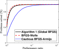
Figure 1: Performance profiles considering 300 starting points for each test problem using the CPU time as performance measurement.

In the following, we evaluate the algorithms based on their ability to properly generate Pareto frontiers. To assess this, we employ the widely recognized Purity and ($\Gamma$ and $\Delta$) Spread metrics. In summary, the Purity metric measures the solver’s ability to identify points on the Pareto frontier, while the Spread metric evaluates the distribution quality of the obtained Pareto frontier. For a detailed explanation of these metrics and their application together with performance profiles, we refer the reader to [14]. The results in Figure 2 indicate that Algorithm 1 performed slightly better in terms of the Purity and $\Delta$-Spread metrics, with no significant difference observed for the $\Gamma$-Spread metric among the three algorithms.

(a) Purity	(b) $\Gamma$-Spread	(c) $\Delta$-Spread

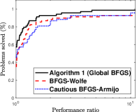
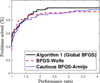
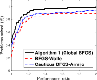
Figure 2: Metric performance profiles: (a) Purity; (b) Spread $\Gamma$; (c) Spread $\Delta$.

The numerical results allow us to conclude that the modifications made to the BFGS method to ensure global convergence for nonconvex problems do not compromise its practical performance.

6 Final remarks

Based on the work of Li and Fukushima [35], we presented a modified BFGS scheme that achieves global convergence without relying on convexity assumptions for the objective function $F$. The global convergence analysis depends only on the requirement of $F$ having continuous Lipschitz gradients. Furthermore, we showed that by appropriately selecting $r_{j}^{k}$ to satisfy Assumption 4.2 and under suitable conditions, the rate of convergence becomes superlinear. We also discussed some practical choices for $r_{j}^{k}$. The introduced modifications preserve the simplicity and practical efficiency of the BFGS method. It is worth emphasizing that the assumptions considered in our approach are natural extensions of those commonly employed in the context of scalar-valued optimization.

Data availability statement
The codes supporting the numerical experiments are freely available in the Github repository, https://github.com/lfprudente/GlobalBFGS.

Conflicts of interest
The authors declare that they have no conflict of interest.

References

• [1] M. A. Ansary and G. Panda. A modified quasi-Newton method for vector optimization problem. Optimization, 64(11):2289–2306, 2015.
• [2] P. B. Assunção, O. P. Ferreira, and L. F. Prudente. Conditional gradient method for multiobjective optimization. Comput. Optim. Appl., 78(3):741–768, 2021.
• [3] J. Y. Bello Cruz, L. R. Lucambio Pérez, and J. G. Melo. Convergence of the projected gradient method for quasiconvex multiobjective optimization. Nonlinear Anal., 74(16):5268–5273, 2011.
• [4] E. Birgin and J. Martínez. Practical Augmented Lagrangian Methods for Constrained Optimization. SIAM, Philadelphia, 2014.
• [5] H. Bonnel, A. N. Iusem, and B. F. Svaiter. Proximal methods in vector optimization. SIAM J. Optim., 15(4):953–970, 2005.
• [6] C. G. Broyden. The Convergence of a Class of Double-rank Minimization Algorithms 1. General Considerations. IMA J. Appl. Math., 6(1):76–90, 1970.
• [7] R. H. Byrd and J. Nocedal. A tool for the analysis of quasi-Newton methods with application to unconstrained minimization. SIAM J. Numer. Anal., 26(3):727–739, 1989.
• [8] L. C. Ceng, B. S. Mordukhovich, and J. C. Yao. Hybrid approximate proximal method with auxiliary variational inequality for vector optimization. J. Optimiz. Theory App., 146(2):267–303, 2010.
• [9] L. C. Ceng and J. C. Yao. Approximate proximal methods in vector optimization. Eur. J. Oper. Res., 183(1):1–19, 2007.
• [10] W. Chen, X. Yang, and Y. Zhao. Conditional gradient method for vector optimization. Comput. Optim. Appl., 85(3):857–896, 2023.
• [11] T. D. Chuong. Generalized proximal method for efficient solutions in vector optimization. Numer. Funct. Anal. Optim., 32(8):843–857, 2011.
• [12] T. D. Chuong. Newton-like methods for efficient solutions in vector optimization. Comput. Optim. Appl., 54(3):495–516, 2013.
• [13] T. D. Chuong, B. S. Mordukhovich, and J. C. Yao. Hybrid approximate proximal algorithms for efficient solutions in vector optimization. J. Nonlinear Convex Anal., 12(2):257–285, 2011.
• [14] A. L. Custódio, J. F. A. Madeira, A. I. F. Vaz, and L. N. Vicente. Direct Multisearch for Multiobjective Optimization. SIAM J. Optim., 21(3):1109–1140, 2011.
• [15] Y.-H. Dai. Convergence properties of the BFGS algorithm. SIAM J. Optim., 13(3):693–701, 2002.
• [16] Y.-H. Dai. A perfect example for the BFGS method. Math. Program., 138(1-2):501–530, 2013.
• [17] J. E. Dennis and J. J. Moré. A characterization of superlinear convergence and its application to quasi-Newton methods. Math. Comp., 28(126):549–560, 1974.
• [18] E. D. Dolan and J. J. Moré. Benchmarking optimization software with performance profiles. Math. Program., 91(2):201–213, 2002.
• [19] G. Eichfelder. Adaptive Scalarization Methods in Multiobjective Optimization. Springer Berlin Heidelberg, 2008.
• [20] N. S. Fazzio and M. L. Schuverdt. Convergence analysis of a nonmonotone projected gradient method for multiobjective optimization problems. Optim. Lett., 13(6):1365–1379, 2019.
• [21] R. Fletcher. A new approach to variable metric algorithms. Comput. J., 13(3):317–322, 1970.
• [22] J. Fliege, L. M. Graña Drummond, and B. F. Svaiter. Newton’s method for multiobjective optimization. SIAM J. Optim., 20(2):602–626, 2009.
• [23] J. Fliege and B. F. Svaiter. Steepest descent methods for multicriteria optimization. Math. Methods of Oper. Res., 51(3):479–494, 2000.
• [24] E. H. Fukuda and L. M. Graña Drummond. On the convergence of the projected gradient method for vector optimization. Optimization, 60(8-9):1009–1021, 2011.
• [25] E. H. Fukuda and L. M. Graña Drummond. Inexact projected gradient method for vector optimization. Comput. Optim. Appl., 54(3):473–493, 2013.
• [26] D. Goldfarb. A family of variable-metric methods derived by variational means. Math. Comput., 24:23–26, 1970.
• [27] M. Gonçalves, F. Lima, and L. Prudente. A study of Liu-Storey conjugate gradient methods for vector optimization. Appl. Math. Comput., 425:127099, 2022.
• [28] M. L. N. Gonçalves, F. S. Lima, and L. F. Prudente. Globally convergent Newton-type methods for multiobjective optimization. Comput. Optim. Appl., 83(2):403–434, 2022.
• [29] M. L. N. Gonçalves and L. F. Prudente. On the extension of the Hager–Zhang conjugate gradient method for vector optimization. Comput. Optim. Appl., 76(3):889–916, 2020.
• [30] L. M. Graña Drummond and A. N. Iusem. A Projected Gradient Method for Vector Optimization Problems. Comput. Optim. Appl., 28(1):5–29, 2004.
• [31] L. M. Graña Drummond, F. M. P. Raupp, and B. F. Svaiter. A quadratically convergent Newton method for vector optimization. Optimization, 63(5):661–677, 2014.
• [32] L. M. Graña Drummond and B. F. Svaiter. A steepest descent method for vector optimization. J. Comput. Appl. Math., 175(2):395–414, 2005.
• [33] K. K. Lai, S. K. Mishra, and B. Ram. On q-Quasi-Newton’s Method for Unconstrained Multiobjective Optimization Problems. Mathematics, 8(4), 2020.
• [34] M. Lapucci and P. Mansueto. A limited memory quasi-Newton approach for multi-objective optimization. Comput. Optim. Appl., 85(1):33–73, 2023.
• [35] D.-H. Li and M. Fukushima. A modified BFGS method and its global convergence in nonconvex minimization. J. Comput. Appl. Math., 129(1):15–35, 2001.
• [36] D.-H. Li and M. Fukushima. On the global convergence of the BFGS method for nonconvex unconstrained optimization problems. SIAM J. Optim., 11(4):1054–1064, 2001.
• [37] L. R. Lucambio Pérez and L. F. Prudente. Nonlinear conjugate gradient methods for vector optimization. SIAM J. Optim., 28(3):2690–2720, 2018.
• [38] L. R. Lucambio Pérez and L. F. Prudente. A Wolfe line search algorithm for vector optimization. ACM Trans. Math. Softw., 45(4):23, 2019.
• [39] N. Mahdavi-Amiri and F. S. Sadaghiani. A superlinearly convergent nonmonotone quasi-newton method for unconstrained multiobjective optimization. Optim. Methods Softw., 35(6):1223–1247, 2020.
• [40] W. F. Mascarenhas. The BFGS method with exact line searches fails for non-convex objective functions. Math. Program., 99(1):49–61, 2004.
• [41] K. Miettinen. Nonlinear multiobjective optimization, volume 12. Springer Science & Business Media, 1999.
• [42] V. Morovati, H. Basirzadeh, and L. Pourkarimi. Quasi-Newton methods for multiobjective optimization problems. 4OR-Q J Oper Res, 16(3):261–294, 2017.
• [43] J. Nocedal and S. J. Wright. Numerical Optimization. Springer, New York, NY, USA, second edition, 2006.
• [44] Z. Povalej. Quasi-Newton’s method for multiobjective optimization. J. Comput. Appl. Math., 255:765–777, 2014.
• [45] M. J. D. Powell. Some global convergence properties of a variable metric algorithm for minimization without exact line searches. Nonlinear Programming, SIAM-AMS Proceedings, 4:53–72, 1976.
• [46] L. F. Prudente and D. R. Souza. A quasi-Newton method with Wolfe line searches for multiobjective optimization. J. Optim. Theory Appl., 194:1107–1140, 2022.
• [47] S. Qu, M. Goh, and F. T. Chan. Quasi-Newton methods for solving multiobjective optimization. Oper. Res. Lett., 39(5):397–399, 2011.
• [48] S. Qu, C. Liu, M. Goh, Y. Li, and Y. Ji. Nonsmooth multiobjective programming with quasi-Newton methods. Eur. J. Oper. Res., 235(3):503–510, 2014.
• [49] D. F. Shanno. Conditioning of quasi-Newton methods for function minimization. Math. Comput., 24:647–656, 1970.
• [50] B. F. Svaiter. The multiobjective steepest descent direction is not Lipschitz continuous, but is Hölder continuous. Oper. Res. Lett., 46(4):430–433, 2018.
• [51] J. Wang, Y. Hu, C. K. Wai Yu, C. Li, and X. Yang. Extended Newton methods for multiobjective optimization: majorizing function technique and convergence analysis. SIAM J. Optim., 29(3):2388–2421, 2019.