Long-range Meta-path Search on Large-scale Heterogeneous Graphs

Abstract

Utilizing long-range dependency, though extensively studied in homogeneous graphs, has not been well investigated on heterogeneous graphs. Addressing this research gap presents two major challenges. The first is to alleviate computational costs while endeavoring to leverage as much effective information as possible in the presence of heterogeneity. The second involves overcoming the well-known over-smoothing issue occurring in various graph neural networks. To this end, we investigate the importance of different meta-paths and introduce an automatic framework for utilizing long-range dependency on heterogeneous graphs, denoted as Long-range Meta-path Search through Progressive Sampling (LMSPS). Specifically, we develop a search space with all meta-paths related to the target node type. By employing a progressive sampling algorithm, LMSPS dynamically shrinks the search space with hop-independent time complexity. Utilizing a sampling evaluation strategy as the guidance, LMSPS conducts a specialized and effective meta-path selection. Subsequently, only effective meta-paths are employed for retraining to reduce costs and overcome the over-smoothing issue. Extensive experiments on various heterogeneous datasets demonstrate that LMSPS discovers effective long-range meta-paths and outperforms the state-of-the-art. Besides, it ranks top-$1$ on the leaderboards of ogbn-mag in Open Graph Benchmark. Our code is available at https://github.com/JHL-HUST/LDMLP.

1 Introduction

Heterogeneous graphs are widely used for abstracting and modeling multiple types of entities and relationships in complex systems by various types of nodes and edges. For instance, the large-scale academic network, ogbn-mag, contains multiple node types, i.e., Paper (P), Author (A), Institution (I), and Field (F), as well as multiple edge types, such as Author $\xrightarrow{\rm writes}$ Paper, Paper$\xrightarrow{\rm cites}$Paper, Author $\xrightarrow{\rm is~{}affiliated~{}with}$ Institution, and Paper$\xrightarrow{\rm has~{}a~{}topic~{}of}$Field. These elements can be combined to build higher-level semantic relations called meta-paths (Sun et al., 2011). For example, PAP is a $2$-hop meta-path representing the co-author relationship, and PFPAPFP is a $6$-hop meta-path related to long-range dependency.

Utilizing long-range dependency is essential for graph representation learning. For homogeneous graphs, many graph neural networks (GNNs) (Li et al., 2019; Bianchi et al., 2020; Alon & Yahav, 2021; Ying et al., 2021) have been developed to gain benefit from long-range dependency. Utilizing long-range dependency is also crucial for heterogeneous graphs. For instance, the Internet movie database (IMDB) contains $21K$ nodes with only $87K$ edges. Such sparsity means each node has only a few directly connected neighbors and requires models to enhance the node embedding from long-range neighbors. The main challenge in using long-range dependency on heterogeneous graphs is how to alleviate costs while striving to effectively utilize information in exponentially increased receptive fields, which is much more challenging compared to homogeneous graphs due to the heterogeneity. In addition, the well-known over-smoothing issue (Li et al., 2018; Keriven, 2022) occurring in many GNNs also needs to be addressed.

Heterogeneous Graph Neural Networks (HGNNs) are popular deep learning techniques for heterogeneous graph representation learning. Their key idea is to aggregate valuable neighbor information based on a range of relations to enhance the semantics of vertices. Traditional HGNNs are typically classified into two categories: metapath-free methods and metapath-based methods. Most metapath-free HGNNs (Zhu et al., 2019; Hong et al., 2020; Hu et al., 2020b; Lv et al., 2021) utilize information from $l$-hop neighborhoods through stacking $l$ layers. However, on large-scale heterogeneous graphs, the number of nodes in receptive fields grows exponentially with the number of layers, making them hard to expand to large hops. A recent work (Mao et al., 2023) employs the graph transformer (Ying et al., 2021) to learn heterogeneous graphs, which can only exploit long-range dependency in small datasets due to the quadratic complexity of transformer (He et al., 2023).

Metapath-based HGNNs (Wang et al., 2019; Fu et al., 2020; Ji et al., 2021; Yang et al., 2023) obtain information from $l$-hop neighborhoods by utilizing single-layer structures and meta-paths with maximum hop $l$, i.e., all meta-paths no more than $l$ hops. To exploit long-range dependency, the maximum hop needs to be large enough as there are no stacking layers. However, the number of meta-paths also grows exponentially with maximum hop $l$, corresponding to exponential receptive fields associated with layers in metapath-free methods. For instance, on ogbn-mag, to gain a $3$-hop meta-path based on the $2$-hop meta-path PAP, the next node type has three choices (A, P, and F). For each additional hop, the number of possible meta-paths increases exponentially. Hence, utilizing long-range dependencies on large-scale heterogeneous graphs has not been resolved yet.

This paper investigates the importance of various meta-paths and makes two key observations: (1) A small number of meta-paths dominate the performance, and (2) certain meta-paths can have a negative impact on performance. The second observation explains why few HGNNs gain benefit from long-range neighbors. Different from homogeneous graphs, messages on heterogeneous graphs can be noisy or redundant for specific tasks, and the presence of long-range dependencies makes it more challenging to exclude negative heterogeneous information, even with the use of attention mechanisms. These findings highlight the opportunity to leverage long-range dependencies by selectively utilizing effective meta-paths.

Motivated by the observations mentioned above, we propose a novel method called Long-range Meta-path Search through Progressive Sampling (LMSPS). LMSPS focuses on meta-path search and aims to reduce the exponentially growing meta-paths to a subset that is specifically effective for the given dataset and task. LMSPS builds a comprehensive search space initially, including all meta-paths related to the target nodes. Then, it adopts a progressive sampling algorithm to reduce the search space. Finally, LMSPS selects the top-$M$ meta-paths from the reduced search space based on a sampling evaluation strategy. This search stage reduces the exponential number of meta-paths to a constant for retraining. Experimental results on both real-world and manual sparse large-scale datasets demonstrate that LMSPS outperforms existing state-of-the-art methods for heterogeneous graph representation learning.

Our main contributions are summarized as follows:

• We propose a novel meta-path search framework termed LMSPS, that is the first HGNNs to utilize long-range dependency in large-scale heterogeneous graphs.

• To search for effective meta-paths efficiently, we introduce a novel progressive sampling algorithm to reduce the search space dynamically and a sampling evaluation strategy for meta-path selection.

• Moreover, the searched meta-paths of LMSPS can be generalized to other HGNNs to boost their performance.

2 Preliminaries

Heterogeneous graph (Sun & Han, 2012). A heterogeneous graph is defined as $\mathcal{G}=\{\mathcal{V},\mathcal{E},\mathcal{T},\mathcal{R},f_{\mathcal{T}},f_{\mathcal{R}}\}$ with $|\mathcal{T}{+}\mathcal{R}|{>}2$, where $\mathcal{V}$ denotes the set of nodes, $\mathcal{E}$ denotes the set of edges, $\mathcal{T}$ is the node-type set and $\mathcal{R}$ the edge-type set. Each node $v_{i}\in\mathcal{V}$ is maped to a node type $f_{\mathcal{T}}(v_{i})\in\mathcal{T}$ by mapping function $f_{\mathcal{T}}:\mathcal{V}\rightarrow\mathcal{T}$. Similarly, each edge $e_{t\leftarrow s}\in\mathcal{E}$ ($e_{ts}$ for short) is mapped to an edge type $f_{\mathcal{R}}(e_{ts})\in\mathcal{R}$ by mapping function $f_{\mathcal{R}}:\mathcal{E}\rightarrow\mathcal{R}$.

Meta-path (Sun et al., 2011). A meta-path $P$ is a composite relation that consists of multiple edge types, i.e., $P\triangleq c_{1}\stackrel{{\scriptstyle r_{12}}}{{\longleftarrow}}c_{2}\cdots c_{l-1}\stackrel{{\scriptstyle r_{(l-1)l}}}{{\longleftarrow}}c_{l}$ ($P=c_{1}c_{2}\cdots c_{l}$ for short), where $c_{1},\dots,c_{l}\in\mathcal{T}$ and $r_{12},\dots,r_{(l-1)l}\in\mathcal{R}$.

A meta-path $P$ corresponds to multiple meta-path instances in the underlying heterogeneous graph. For example, meta-path PAP corresponds to all paths of co-author relationships on the heterogeneous graph. In HGNNs, using meta-paths means selectively aggregating neighbors on the meta-path instances.

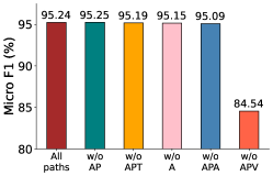
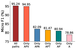
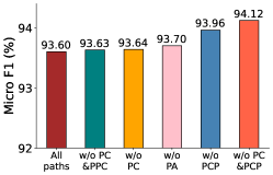
Figure 1: Analysis of the importance of different meta-paths. (a) illustrates the results after removing a single meta-path on DBLP. (b) shows the performance of utilizing a single meta-path on DBLP (c) illustrates the performance after removing a part of meta-paths on ACM.

3 Related Works

Heterogeneous Graph Neural Networks. HGNNs are proposed to learn rich and diverse semantic information on heterogeneous graphs. Several HGNNs (Li et al., 2021a; Ji et al., 2021; Lv et al., 2021; Mao et al., 2023) have involved high-order semantic aggregation. However, their methods are not applied to large-scale datasets due to relatively high costs. Additionally, many HGNNs (Yun et al., 2019; Hu et al., 2020b; Wang et al., 2019; Ji et al., 2021) have implicitly learned meta-paths by attention. However, few work employs the discovered meta-paths to generate final results, let alone generalize them to other HGNNs to demonstrate their effectiveness. For example, GTN (Yun et al., 2019) and HGT (Hu et al., 2020b) only list the discovered meta-paths. HAN (Wang et al., 2019), HPN (Ji et al., 2021) and MEGNN (Chang et al., 2022) validate the importance of discovered meta-paths by experiments not directly associated with the learning task. GraphMSE (Li et al., 2021b) is the only work that shows the performance of the discovered meta-paths. However, they are not as effective as the full meta-path set. Consequently, their learned meta-paths are not effective enough. Unlike these methods, the meta-paths searched by LMSPS not only enable it to outperform existing HGNNs but also are effective on other HGNNs. Furthermore, the meta-paths searched by LMSPS enable it to efficiently leverage long-range dependencies on large-scale datasets by only utilizing effective semantic information.

Meta-structure Search on Heterogeneous Graphs. Recently, some works have attempted to utilize neural architecture search (NAS) to discover meta-structures. GEMS (Han et al., 2020) is the first NAS method on heterogeneous graphs, which utilizes an evolutionary algorithm to search meta-graphs for recommendation tasks. DiffMG (Ding et al., 2021) searches for meta-graphs by a differentiable algorithm to conduct an efficient search. PMMM (Li et al., 2023) performs a stable search to find meaningful meta-multigraphs. However, meta-path-based HGNNs are mainstream methods (Schlichtkrull et al., 2018; Zhang et al., 2019; Wang et al., 2019; Fu et al., 2020), while meta-graph-based HGNNs are specialized. So, their searched meta-graphs are extremely difficult to generalize to other HGNNs. RL-HGNN (Zhong et al., 2020) proposes a reinforcement learning (RL)-based method to find meta-paths. On recommendation tasks, RMS-HRec (Ning et al., 2022) also proposes an RL-based meta-path selection strategy to discover meta-paths. However, how to search meta-structures on large-scale heterogeneous graphs is a non-trivial problem, and how to search meta-structures that are effective across different HGNNs is also challenging. All the above works have not addressed both problems.

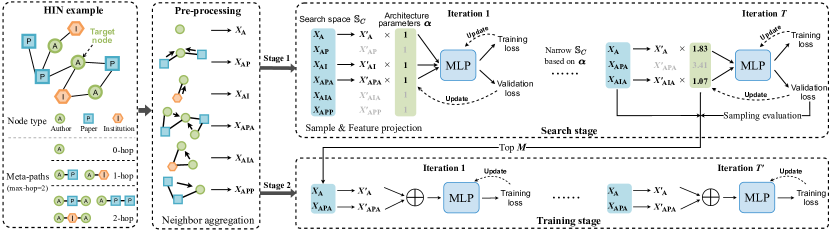
Figure 2: The overall framework of LMSPS. Based on the progressive sampling and sampling evaluation in the search stage, the training stage employs $M$ effective meta-paths instead of the full $K$ target-node-related meta-paths. This figure exhibits aggregation of meta-paths with maximum hop $2$, i.e., $0$, $1$, and $2$-hop meta-paths. The weight updates of feature projection are not shown for ease of illustration.

4 Motivation of Meta-path Search

Many HGNNs (Yun et al., 2019; Li et al., 2021b; Chang et al., 2022; Yang et al., 2023) employ all target-node-related meta-paths for heterogeneous graph representation learning. However, the contribution of each meta-path is under-explored. In this section, we conduct an in-depth study of different meta-paths and gain two crucial conclusions through experiments, helping us to propose the key idea of leveraging long-range dependencies effectively.

SeHGNN (Yang et al., 2023) employs attention mechanisms to fuse all the target-node-related meta-paths and outperforms the existing HGNNs. It has an important finding that models with single-layer structures and long meta-paths outperform those with multi-layers and short meta-paths, indicating the importance of long-range meta-paths. However, because the number of meta-paths increases exponentially with maximum hops, SeHGNN has to use a small maximum hop of $2$ for large-scale datasets like ogbn-mag (Hu et al., 2021) to save memory and reduce costs, which is insufficient as shown in Table 5 of the experiments.

We analyze the importance of different meta-paths for SeHGNN on two widely-used real-world datasets DBLP and ACM from HGB (Lv et al., 2021). All results are the average of $10$ times running with different random initializations. As the number of meta-paths exponentially increases with the maximum hop, in exploratory experiments, we set the maximum hop $l=2$ for ease of illustration. Then the meta-path sets are $\{$A, AP, APA, APT, APV$\}$ on DBLP, and $\{$P, PA, PC, PP, PAP, PCP, PPA, PPC, PPP$\}$ on ACM.

In each experiment on DBLP, we remove one meta-path and compare the performance with the result of leveraging the full meta-path set to analyze the importance of the removed meta-path. As shown in Figure 1 (a), removing either A or AP or APA or APT has little impact on the final performance. However, removing APV results in severe degradation in performance, demonstrating APV is the critical meta-path on DBLP when $l=2$. We further retain one meta-path and remove others as shown in Figure 1 (b). The performance of utilizing APV is only slightly degraded compared to the full meta-paths set. Consequently, we obtain the first finding: A small number of meta-paths provide major contributions. In each experiment on ACM, we remove some meta-paths to analyze their impact on the final performance. Results in Figure 1 (c) show that the performance of SeHGNN improves after removing a part of meta-paths. For example, after removing PC and PCP, the Micro-F1 scores improve by $0.52\%$. So, we can conclude the second finding: Certain meta-paths can have a negative impact for heterogeneous graphs.

The second finding is reasonable because heterogeneous information is not consistently beneficial for various tasks compared to homogeneous information. It is supported by the fact that various recent HGNNs (Ding et al., 2021; Li et al., 2023; Yang et al., 2023) have removed some edge types to exclude corresponding heterogeneous information during pre-processing based on substantial domain expertise or empirical findings. This observation explains why most HGNNs use a maximum hop of $2$, i.e., it is hard to exclude negative information under larger maximum hops. Additionally, because SeHGNN employs an attention mechanism, the performance degradation indicates the attention mechanism has limitations in dealing with noise.

Motivated by the above findings, we can employ effective meta-paths instead of the full meta-path set without sacrificing performance. Although the number of meta-paths grows exponentially with the maximum hop, the proportion of effective meta-paths is small, which is similar to the $80/20$ rule of Pareto principle (Sanders, 1987; Erridge, 2006). To keep efficiency while trading off the performance, we choose a fixed number of meta-paths (like $30$) over all datasets, avoiding computation on numerous noisy or redundant meta-paths when the maximum hop is large.

5 The Proposed Method

The key point of our LMSPS is to utilize a search stage to reduce the exponentially increased meta-paths to a subset that is effective to the current dataset and task. It can overcome the main challenges of utilizing long-range dependency on heterogeneous graphs. First, utilizing effective meta-paths instead of all meta-paths alleviates computational and memory costs while keeping effective heterogeneous information. Second, each target node only aggregates neighbors on the path instances of effective meta-paths. Because the proportion of effective meta-paths is small and each node has a different neighborhood condition, each target node aggregates different neighbors under the constraints of effective meta-path instances. In this way, the over-smoothing issue can also be overcome.

Then, the main challenge becomes how to discover effective meta-paths. Because the exponential meta-paths severely challenge the efficiency and effectiveness of meta-path search, we propose a progressive sampling algorithm and a sampling evaluation strategy to respectively overcome the two challenges. Figure 2 illustrates the overall framework of LMSPS, which consists of a super-net in the search stage and a target-net in the training stage.

The super-net aims to automatically discover effective meta-paths for specific datasets or tasks, so the search results should not be affected by specific modules. Based on this consideration, we develop a simple MLP-based instead of transformer-based architecture for meta-path search because the former involves fewer human interventions (Tolstikhin et al., 2021; Wang et al., 2022). The super-net contains five blocks: neighbor aggregation, feature projection, progressive sampling search, sampling evaluation, and MLP.

5.1 Progressive Sampling Search

Let $\mathbb{P}=\{P_{1},\cdots,P_{k},\cdots,P_{K}\}$ be the initial search space with all $K$ target-node-related meta-paths. Let $\bm{X}^{c_{i}}$ be the raw feature matrix of all nodes belonging to type $c_{i}$, and $\bm{\hat{A}}_{c_{i},c_{i}+1}$ be the row-normalized adjacency matrix between node type $c_{i}$ and $c_{i+1}$. The neighbor aggregation block follows SeHGNN (Yang et al., 2023), which pre-process the heterogeneous graph into regular-shaped tensors for target nodes. Specifically, it uses the multiplication of adjacency matrices to calculate the final contribution weight of each metapath-based neighbor to targets. As shown in Figure 2, the neighbor aggregation process of $l$-hop meta-path $P_{k}=c_{0}c_{1}c_{2}\ldots c_{l}$ is:

$$\bm{X}_{k}=\begin{cases}\bm{X}^{c_{0}}&l=0\\ \bm{\hat{A}}_{c_{0},c_{1}}\bm{\hat{A}}_{c_{1},c_{2}}\cdots\bm{\hat{A}}_{c_{l-1},c_{l}}\bm{X}^{c_{l}}&l>0\end{cases},$$ (1)

where $\bm{X}_{k}$ is the feature matrices of meta-path $P_{k}$, and $c_{0}$ is the target node type. Then, an MLP-based feature projection block is used to project different feature matrices into the same dimension, namely, $\bm{X}_{k}^{\prime}={\rm MLP}_{k}(\bm{X}_{k})$.

To automatically discover meaningful meta-paths for various datasets or tasks without prior, our search space contains all target-node-related meta-paths, severely challenging the efficiency and effectiveness of searching. To overcome the efficiency challenge, LMSPS utilizes a progressive sampling algorithm to sample a part of meta-paths in each iteration and progressively shrink the search space.

Specifically, LMSPS assigns one architecture parameter to each meta-path. Let $\bm{\alpha}=\{\alpha_{1},\cdots,\alpha_{k},\cdots,\alpha_{K}\}\in\mathbb{R}^{K}$ be corresponding architecture parameters of $K$ meta-paths. We use a Gumbel-softmax (Maddison et al., 2016; Dong & Yang, 2019) over architecture parameters $\alpha_{k}$ to calculate the strength of different meta-paths:

$$q_{k}=\frac{\exp\left[\left(\alpha_{k}+u_{k}\right)/\tau\right]}{\sum^{K}_{j=1}\exp\left[\left(\alpha_{j}+u_{j}\right)/\tau\right]},$$ (2)

where $q_{k}$ is the path strength, representing the relative importance of meta path $P_{k}$. $u_{k}=-\log\left(-\log\left(U\right)\right)$ where $U\sim\operatorname{Uniform}(0,1)$, and $\tau$ is the temperature controlling the continuous relaxation’s extent.

The progressive sampling algorithm uses the path strength to progressively narrow the search space from $K$ to $V$ to exclude useless meta-paths. Generally, $K\gg V$ under a large maximum hop. Let $\widetilde{q}_{C}$ be the $C$-th largest path strength of $\mathbb{Q}=\{q_{1},\cdots,q_{k},\cdots,q_{K}\}$. During the search stage, the search space retains all meta-paths no less than $\widetilde{q}_{C}$. The dynamic search space can be formulated as:

$$\mathbb{S}_{C} =\{k|q_{k}\geq\widetilde{q}_{C},\forall 1\leq k\leq K\},$$ (3)

$$\text{where}\,\,C =\lceil\lambda(K-V)\rceil+V.$$ (4)

Here $C$ is the search space size, $\mathbb{S}_{C}$ consists of the indexes of retained meta-paths, and $\lceil\cdot\rceil$ indicates the rounding symbol. $\lambda\in[0,1]$ is a parameter controlling the number of retrained meta-paths and decreases from $1$ to $0$ as the epoch increases.

As the search stage aims to determine top-$M$ meta-paths, we sample $M$ meta-paths from dynamic search space in each iteration. In each iteration, only parameters on the $M$ activated meta-paths are updated, and the rest remain unchanged. Therefore, the search cost is relevant to $M$ instead of $K$. The forward propagation can be expressed as:

$$\bm{Z} ={\rm MLP}\Big{(}\sum_{k\in\mathbb{S}}q_{k}^{\prime}\cdot{\rm MLP}_{k}(\bm{X}_{k})\Big{)},$$ (5)

$$\text{where}\,\,\mathbb{S} ={\rm UniformSample}(\mathbb{S}_{C},M).$$ (6)

Here $q_{k}^{\prime}=\exp\left[\left(\alpha_{k}+u_{k}\right)/\tau\right]/\sum_{k\in\mathbb{S}}\exp\left[\left(\alpha_{j}+u_{j}\right)/\tau\right]$ indicates the path strength of activated meta-paths, and UniformSample$(\mathbb{S}_{C},M)$ indicates a set of $M$ elements chosen randomly from set $\mathbb{S}_{C}$ without replacement via a uniform distribution.

The parameter update in the super-net involves a bilevel optimization problem (Anandalingam & Friesz, 1992; Colson et al., 2007; Xue et al., 2021).

$$\min_{\bm{\alpha}}\,\, \mathcal{L}_{val}(\mathbb{S},\bm{\omega}^{*}(\bm{\alpha}),\bm{\alpha}),$$ (7)

s.t. $$\bm{\omega}^{*}(\bm{\alpha})=\mathrm{argmin}_{\bm{\omega}}\,\mathcal{L}_{train}(\mathbb{S},\bm{\omega},\bm{\alpha}).$$ (8)

Here $\mathcal{L}_{train}$ and $\mathcal{L}_{val}$ denote the training and validation loss, respectively. $\bm{\alpha}$ is the architecture parameters calculating the path strength. $\bm{\omega}$ is the network weights in MLP. Following the NAS-related works in the computer vision field (Liu et al., 2019b; Xie et al., 2019; Yao et al., 2020), we address this issue by first-order approximation. Specifically, we alternatively freeze architecture parameters $\bm{\alpha}$ when training $\bm{\omega}$ on the training set and freeze $\bm{\omega}$ when training $\bm{\alpha}$ on the validation set.

The progressive sampling strategy can contribute to a more compact search space specifically driven by the current HIN and task, leading to a more effective meta-path discovery. Additionally, it can overcome the deep coupling issue (Guo et al., 2020) because of the randomness in each iteration.

Table 1: Time complexity comparison of every training epoch. $\dagger$ means time complexity under small-scale datasets and full-batch training.

Method	Feature projection	Neighbor aggregation	Semantic fusion	Total
HAN	$O(N(rd)^{l}F^{2})$	$O(N(rd)^{l}F)$	$O(Nr^{l}F^{2})$	$O(N(rd)^{l}F^{2})$
Simple-HGN	$O(N(rd)^{l}F^{2})$	$O(N(rd)^{l}F)$	-	$O(N(rd)^{l}F^{2})$
Simple-HGN†	$O(NrdlF^{2})$	$O(NrdlF)$	-	$O(NrdlF^{2})$
SeHGNN	$O(Nr^{l}F^{2})$	-	$O(Nr^{l}F^{2}+Nr^{2l}F)$	$O(N(r^{l}F^{2}+r^{2l}F))$
LMSPS-search	$O(NMF^{2})$	-	$O(NMF^{2})$	$O(NMF^{2})$
LMSPS-train	$O(NMF^{2})$	-	$O(NMF^{2})$	$O(NMF^{2})$

5.2 Sampling Evaluation

After the completion of progressive sampling search, the search space is narrowed from $K$ to $V$. Traditional methods in the computer vision field directly derive the final architecture based on the architecture parameters (Liu et al., 2019b; Xie et al., 2019; Yao et al., 2020). However, a recent research (Wang et al., 2021) has verified that architecture parameters are not effective enough to indicate the strength of the candidates. In addition, because different meta-paths could be noisy or redundant to each other, top-$M$ meta-paths are not necessarily the optimal solution when their importance is calculated independently. Based on this consideration, we propose a novel sampling evaluation strategy. Specifically, using path strength as the probability, we sample $M$ meta-paths from the compact search space $\mathbb{S}_{V}$ to evaluate their overall performance. The sampling evaluation is repeated $200$ times to filter out the meta-path set with the lowest validation loss. This stage is not time-consuming because the evaluation does not involve weight training. This sampling process can be represented as:

$$\bar{\mathbb{S}}={\rm DiscreteSample}(\mathbb{S}_{V},M,\bar{\mathbb{Q}}).$$ (9)

Here, DiscreteSample$(\mathbb{S}_{V},M,\bar{\mathbb{Q}})$ indicates a set of $M$ elements chosen from the set $\mathbb{S}_{V}$ without replacement via discrete probability distribution $\bar{\mathbb{Q}}$. $\bar{\mathbb{Q}}$ is the set of relative path strength calculated by architecture parameters of the $V$ meta-paths based on Equation 2. The overall search algorithm and more discussion are shown in Appendix B.

Thereafter, the retained meta-path set is recorded as $\mathbb{S}_{M}=\mathrm{argmin}_{\bar{\mathbb{S}}}\,{\cal L}_{val}(\bar{\mathbb{S}},\bm{\omega}^{*},\bm{\alpha}^{*})$. The forward propagation of the target-net for representation learning can be formulated as:

$$\vspace{-2pt}\hat{\bm{Z}}={\rm MLP}\Big{(}\operatorname*{\scalebox{1.0}[1.5]{$\parallel$}}_{k\in\mathbb{S}_{M}}{\rm MLP}_{k}(\bm{X}_{k})\Big{)}.\vspace{-4pt}$$ (10)

Here, $\operatorname*{\scalebox{1.0}[1.5]{$\parallel$}}$ denotes the concatenation operation. Unlike existing HGNNs, the architecture of the target-net does not contain neighbor attention and semantic attention. Instead, the parametric modules consist of pure MLPs. The training objective is shown in Appendix A.

5.3 Time Complexity Analysis

Following the convention (Chiang et al., 2019; Yang et al., 2023), we compare the time complexity of LMSPS with HAN (Wang et al., 2019), Simple-HGN (Lv et al., 2021), and SeHGNN (Yang et al., 2023) under mini-batch training with the total $N$ target nodes. All methods employ $l$-hop neighborhood. For simplicity, we assume that the number of features is fixed to $F$ for all layers. The average degree of each node is $rd$, where $r$ is the number of edge types and $d$ is the number of edges connected to the node for each edge type. The complexity analysis is summarized in Table 1. Because HAN and Simple-HGN require neighbor aggregation during training, and the number of neighbors grows exponentially with hops. So, they have neighbor aggregation costs of $O((rd)^{l})$. SeHGNN employs a pre-processing step to avoid the training cost of neighbor aggregation. However, the exponential meta-paths cause SeHGNN to suffer from $O(r^{l})$ costs in semantic aggregation. Unlike the above methods, LMSPS samples $M$ meta-paths in each iteration of the search stage and employs $M$ effective meta-paths in the training stage to avoid exponential costs. Generally, we have $O((rd)^{l})\gg O(r^{l})=O(K)\gg O(M)$ when maximum hop $l$ is large. The time complexity of LMSPS is a constant when $N$ and $F$ are determined, which is the key point for utilizing long-range meta-paths.

6 Experiments and Analysis

This section evaluates the benefits of our method against state-of-the-art models on eight heterogeneous datasets. We aim to answer the following questions: Q1. How does LMSPS perform compared with state-of-the-art baselines? Q2. Does LMSPS perform better on sparser heterogeneous graphs? Q3. Can LMSPS overcome the over-smoothing and noise issues? Q4. Are the searched meta-paths effective on other models? More ablation studies and hyper-parameter studies are provided in Appendix D.6 and D.7.

Table 2: Test accuracy ($\%$) on the ogbn-mag compared with other methods on the OGB leaderboard. See main text for details of label and ms.

Method	Test accuracy
Random	$35.14\pm 3.78$
MLP (Hu et al., 2020a)	$26.92\pm 0.26$
GraphSAGE (Hamilton et al., 2017)	$46.78\pm 0.67$
RGCN (Schlichtkrull et al., 2018)	$47.37\pm 0.48$
HGT (Hu et al., 2020b)	$49.27\pm 0.61$
NARS (Yu et al., 2020)	$50.88\pm 0.12$
SeHGNN (Yang et al., 2023)	$51.79\pm 0.24$
LMSPS	$\textbf{ 54.83}\pm\textbf{ 0.20 }$
SAGN (Sun et al., 2021)+label	$51.17\pm 0.32$
GAMLP (Zhang et al., 2022)+label	$51.63\pm 0.22$
SeHGNN+label	$53.99\pm 0.18$
LMSPS +label	$\textbf{55.10}\pm\textbf{ 0.11}$
SeHGNN+label+ms	$56.71\pm 0.14$
LMSPS +label+ms	$\textbf{57.84}\pm\textbf{ 0.22}$

Table 3: Micro-F1 ($\%$) of LMSPS and baselines on three representative datasets, i.e., DBLP, IMDB, and ACM, from HGB benchmark. All methods do not employ data enhancements like label aggregation.

Method	DBLP	IMDB	ACM
RSHN (Zhu et al., 2019)	$93.81\pm 0.55$	$64.22\pm 1.03$	$90.32\pm 1.54$
HetSANN (Hong et al., 2020)	$80.56\pm 1.50$	$57.68\pm 0.44$	$89.91\pm 0.37$
GTN (Yun et al., 2019)	$93.97\pm 0.54$	$65.14\pm 0.45$	$91.20\pm 0.71$
HGT (Hu et al., 2020b)	$93.49\pm 0.25$	$67.20\pm 0.57$	$91.00\pm 0.76$
Simple-HGN (Lv et al., 2021)	$94.46\pm 0.22$	$67.36\pm 0.57$	$93.35\pm 0.45$
HINormer (Mao et al., 2023)	$94.94\pm 0.21$	$67.83\pm 0.34$	$-$
RGCN (Schlichtkrull et al., 2018)	$92.07\pm 0.50$	$62.05\pm 0.15$	$91.41\pm 0.75$
HetGNN (Zhang et al., 2019)	$92.33\pm 0.41$	$51.16\pm 0.65$	$86.05\pm 0.25$
HAN (Wang et al., 2019)	$92.05\pm 0.62$	$64.63\pm 0.58$	$90.79\pm 0.43$
MAGNN (Fu et al., 2020)	$93.76\pm 0.45$	$64.67\pm 1.67$	$90.77\pm 0.65$
SeHGNN (Yang et al., 2023)	$95.24\pm 0.13$	$68.21\pm 0.32$	$93.87\pm 0.50$
DiffMG (Ding et al., 2021)	$94.20\pm 0.36$	$59.75\pm 1.23$	$88.07\pm 3.04$
PMMM (Li et al., 2023)	$95.14\pm 0.22$	$67.58\pm 0.22$	$93.71\pm 0.17$
LMSPS	$\textbf{95.66}\pm\textbf{0.20}$	$\textbf{68.70}\pm\textbf{0.26}$	$\ \textbf{94.69}\pm\textbf{0.36}$

6.1 Datasets and Baselines

We evaluate LMSPS on the representative large-scale dataset ogbn-mag from OGB challenge (Hu et al., 2021), and three widely-used heterogeneous graphs including DBLP, IMDB, and ACM from HGB benchmark (Lv et al., 2021) on the node classification task. Please see Appendix D.1 for details of all datasets. For the ogbn-mag dataset, the results are compared to the OGB leaderboard, and all scores are the average of $10$ separate training. For the three datasets from HGB, the results are compared to the baseline scores from the HGB paper and several recent advanced methods. Following the convention (Lv et al., 2021; Yang et al., 2023), all scores are the average of $5$ separate local data partitions. GEMS (Han et al., 2020) and RMS-HRec (Ning et al., 2022) are ignored because they are designed for recommendation tasks. RL-HGNN (Zhong et al., 2020) is omitted due to a lack of source code. HINormer (Mao et al., 2023) also doesn’t provide source code but uses two datasets from HGB, we show its reported results.

6.2 Training Details

We set the number of selected meta-paths $M=30$ for all datasets. The final search space $V=60$. The maximum hop is $6$ for ogbn-mag, DBLP and $5$ for IMDB, ACM. All $K$ architecture parameters $\alpha_{1},\alpha_{2},\cdots,\alpha_{K}$ are initialized as $1$s. For searching in the super-net, we train for $200$ epochs. To train the target-net, we use an early stop mechanism based on the validation performance to promise full training. See Appendix D.2 for more details.

6.3 Performance Comparison

Results on Ogbn-mag. To answer Q1, we report the test accuracy of our proposed LMSPS and baselines in Table 3. Random means the result of replacing our searched meta-paths with $30$ random meta-paths. We show the average result of 20 random samples. Because ogbn-mag is much more challenging than other datasets, existing methods usually use extra tricks. label indicates a kind of data augmentation utilizing labels as extra inputs to provide enhancements (Wang & Leskovec, 2020; Shi et al., 2021; Yang et al., 2023). ms means using multi-stage learning  (Li et al., 2018; Sun et al., 2020). It can be seen that LMSPS achieves state-of-the-art performance under each condition. For example, LMSPS outperforms the SOTA method SeHGNN by a large margin of $3.04\%$. The advantage of LMSPS compared to SeHGNN mainly comes from the unique ability to selectively leverage effective heterogeneous information under larger receptive fields, indicating the necessity of long-range meta-paths. SeHGNN shows the results with extra embeddings as an enhancement in the original paper. Though we cannot compare results with this trick due to the untouchability of its embedding file, LMSPS still outperforms their best result.

Performance on HGB Benchmark. Table 3 shows the Micro-F1 scores of LMSPS and baselines. The 1st, 2nd, and 3rd blocks are metapath-free, metapath-based, and NAS-based methods, respectively. The 4th block is our method. Every block contains a method yielding highly competitive performance, indicating that the HGNN field is very active and each mechanism has its advantage. Nevertheless, LMSPS can still consistently perform best on all three datasets.

6.4 Necessity of Long-range Dependency

To answer Q2 and explore the necessity of long-range dependency on heterogeneous graphs, we construct four large-scale datasets with high sparsity based on ogbn-mag. To avoid inappropriate preference seed settings of randomly removing, we construct fixed heterogeneous graphs by limiting the maximum in-degree related to edge type. Specifically, we gradually reduce the maximum in-degree related to edge type in ogbn-mag from $50$ to $5$ but leave all nodes unchanged. Details of the four datasets are listed in Appendix D.1. The test accuracy of LMSPS and SOTA method SeHGNN are shown in Table 4. LMSPS outperforms SeHGNN more significantly with the increasing sparsity. In addition, the leading gap of LMSPS over SeHGNN is more than $4.7\%$ on the highly sparse dataset ogbn-mag-5. The main difference between SeHGNN and LMSPS is that the former cannot utilize large hops and only use hop $2$ while the latter has a maximum hop of $6$, demonstrating that long-range dependencies are more effective with increased sparsity and decreased direct neighbors on heterogeneous graphs.

Table 4: Results of LMSPS and SeHGNN on the sparse large-scale heterogeneous graphs. $\bm{\uparrow}$ means the improvements in test accuracy.

Dataset	SeHGNN	LMSPS	$\bm{\uparrow}$
ogbn-mag-$5$	$36.04\pm 0.64$	$40.82\pm 0.42$	4.78
ogbn-mag-$10$	$38.27\pm 0.19$	$42.30\pm 0.23$	4.03
ogbn-mag-$20$	$39.18\pm 0.09$	$42.65\pm 0.17$	3.47
ogbn-mag-$50$	$39.50\pm 0.13$	$42.82\pm 0.16$	3.32

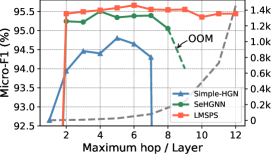
(a) Micro-F1

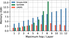
(b) GPU memory cost

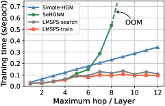
(c) Time cost

Figure 3: Illustration of (a) performance, (b) memory cost, (c) average training time of Simple-HGN, SeHGNN, and LMSPS relative to the maximum hop or layer on DBLP. The gray dotted line in (a) indicates the number of target-node-related meta-paths under different maximum hops, which is exponential.

6.5 Analysis on Large Maximum Hops

To answer Q3, we conduct experiments to compare the performance, memory, and efficiency of LMSPS with the best metapath-free method with source code, Simple-HGN (Lv et al., 2021), and the best metapath-based method, SeHGNN (Yang et al., 2023), on DBLP. Figure 3 (a) shows that LMSPS has consistent performance with the increment of maximum hop. The failure of Simple-HGN demonstrates its attention mechanism can not overcome the over-smoothing issue or eliminate the effects of noise under large hop. Figure 3 (b), (c) illustrate each training epoch’s average memory and time costs relative to the maximum hop or layer. We can observe that the consumption of SeHGNN exponentially grows, and the consumption of Simple-HGN linearly increases, which is consistent with their time complexity as listed in Table 1. At the same time, LMSPS has almost constant consumption as the maximum hop grows. Figure 3 (c) shows the time cost of LMSPS in the search stage, which also approximates a constant when the number of meta-paths is larger than $M=30$.

Table 5: Experiments on ogbn-mag to analyze the performance of SeHGNN and LMSPS under different maximum hops. #MP is the number of corresponding meta-paths of different maximum hops. “$OOM$” means out of memory.

Max hop	SeHGNN		LMSPS
(#MP)	Time (s)	Test accuracy	Time (s)	Test accuracy
$1$ $(4)$	$~{}~{}4.35$	$47.18\pm 0.28$	$~{}~{}3.98$	$46.88\pm 0.10$
$2$ $(10)$	$~{}~{}6.44$	$51.79\pm 0.24$	$~{}~{}5.63$	$51.91\pm 0.13$
$3$ $(23)$	$11.28$	$52.44\pm 0.16$	$10.02$	$52.72\pm 0.24$
$4$ $(50)$	$OOM$	$OOM$	$14.34$	$53.43\pm 0.18$
$5$ $(107)$	$OOM$	$OOM$	$14.77$	$53.90\pm 0.19$
$6$ $(226)$	$OOM$	$OOM$	$14.71$	$\textbf{54.83}\pm\textbf{0.20}$

We also compare the performance and training time of LMSPS with SeHGNN under different maximum hops on large-scale dataset ogbn-mag. When the maximum hop $l=1,2,3$, we utilize the full meta-paths set because the number of target-node-related meta-paths is smaller than $M=30$. Following the convention (Lv et al., 2021; Yang et al., 2023), we measure the average time consumption of one epoch for each model. As shown in Table 5, the performance of LMSPS keeps increases as the maximum hop value grows. It indicates LMSPS can overcome the issues caused by utilizing long-range dependency, e.g., over-smoothing and noise. In addition, when the number of meta-paths is larger than $30$, the training time of LMSPS is stable under different maximum hops. More results about efficiency are shown in Appendix D.4.

6.6 Generalization of the Searched Meta-paths

The effective meta-paths mainly depend on the dataset and task instead of the architecture. To demonstrate the effectiveness of searched meta-paths, on the one hand, the meta-paths should be effective in the proposed model. On the other hand, the meta-paths should be effective after being generalized to other HGNNs. Because finding meta-paths that work effectively across various HGNNs is a tough task, it has not been achieved by previous works. To answer Q4, we verify the generalization of our searched meta-path on the most famous HGNN HAN (Wang et al., 2019) and the SOTA method SeHGNN (Yang et al., 2023). The Micro-F1 scores on three representative datasets are shown in Table 6. After simply replacing the original meta-path set with our searched meta-paths and keeping other settings unchanged, the performance of both methods improves rather than decreases, demonstrating the effectiveness of our searched meta-paths. In addition, we have shown the interpretability searched meta-paths in Appendix C and explored the effectiveness of our search algorithm in Appendix D.3.

Table 6: Experiments on the generalization of the searched meta paths. * means using the meta-paths searched in LMSPS.

Method	DBLP	IMDB	ACM
HAN	$92.05\pm 0.62$	$64.63\pm 0.58$	$90.79\pm 0.43$
HAN*	$93.54\pm 0.15$	$65.89\pm 0.52$	$92.28\pm 0.47$
SeHGNN	$95.24\pm 0.13$	$68.21\pm 0.32$	$93.87\pm 0.50$
SeHGNN*	$95.57\pm 0.23$	$68.59\pm 0.24$	$94.46\pm 0.18$

7 Conclusion

This work presented Long-range Meta-path Search through Progressive Sampling (LMSPS) to tackle the challenges of leveraging long-range dependencies in large-scale heterogeneous graphs, i.e., reducing computational costs while effectively utilizing information and addressing the over-smoothing issue. Based on our two observations, i.e., a few meta-paths dominate the performance, and certain meta-paths can have negative impact on performance, LMSPS introduced a progressive sampling search algorithm and a sampling evaluation strategy to automatically identify effective meta-paths, thus reducing the exponentially growing number of meta-paths to a manageable constant. Extensive experiments demonstrated the superiority of LMSPS over existing methods, particularly on sparse heterogeneous graphs that require long-range dependencies. By employing simple MLPs and complex meta-paths, LMSPS offers a novel direction that emphasizes data-dependent semantic relationships rather than relying solely on sophisticated neural architectures. The reproducibility and limitations are discussed in Appendix E and Appendix F, respectively.

Appendix

In the Appendix, we provide additional details and results not included in the main text due to space limitations. We first show the training objective and search algorithm of LMSPS and explore the algorithm’s effectiveness. Secondly, for interpretability, the searched meta-paths are listed and analyzed. Thirdly, we display more experimental details, explore the training efficiency of LMSPS and compare LMSPS with baselines on Freebase. Ablation studies and hyperparameter studies are also conducted. Finally, we discuss the reproducibility and limitations of our research work.

Appendix A Searching and Training Objective

Following the convention (Lv et al., 2021; Li et al., 2023; Yang et al., 2023; Mao et al., 2023), we concentrate on semi-supervised node classification under the transductive setting and leave other downstream tasks related to heterogeneous graph representation learning as future work. An MLP layer is appended after the main module of LMSPS, which reduces the dimension of node-level representations of a heterogeneous graph to the number of classes:

$$\bar{\bm{Y}} =\text{softmax}(\bm{Z}\bm{\omega}_{o}),$$ (11)

where $\bm{\omega}_{o}\in\mathbb{R}^{d_{o}\times N}$ is the output weight matrix, $d_{o}$ is the dimension of output node representations, and $N$ is the number of classes. Then, the cross-entropy loss is used over all labeled nodes:

$$\mathcal{L} =-\sum\nolimits_{v\in\mathcal{V}_{L}}\sum\nolimits_{n=1}^{N}\bm{y}_{v}[n]\log\bar{\bm{y}}_{v}[n],$$ (12)

where $\mathcal{V}_{L}$ denotes the set of labeled nodes, $\bm{y}_{v}$ is a one-hot vector indicating the label of node $v$, and $\bar{\bm{y}}_{v}$ is the predicted label for the corresponding node in $\bar{\bm{Y}}$. In the search stage, $\mathcal{V}_{L}$ is the training set when updating $\bm{\omega}$ and the validation set when updating $\bm{\alpha}$. In the training stage, $\mathcal{V}_{L}$ is the training set, and $\omega$ is reinitialized and trained.

Algorithm 1 The search algorithm of LMSPS

Input: meta-path sets $\mathbb{P}=\{P_{1},\cdots,P_{K}\}$; number of sampling meta-paths $M$; number of training iterations $T$; number of sampling evaluation $E$
Parameter: Network weights $\bm{\omega}$ in ${\rm MLP}_{k}$ for feature projection and ${\rm MLP}$ for downstream tasks; architecture parameters $\bm{\alpha}=\{\alpha_{1},\cdots,\alpha_{K}\}$
Output: The index set of selected meta-paths $\mathbb{S}_{M}$

1:  % Neighbor aggregation

2:  Calculate neighbor aggregation of raw features for each $P_{k}\in\mathbb{P}$ based on Equation 1

3:  while $t<T$ do

4:     % Path strength

5:     Calculate the path strength of all meta-paths based on Equation 2

6:     % Dynamic search space

7:     Calculate the current search space $\mathbb{S}_{C}$ based on Equations 3 and 4

8:     % Sampling

9:     Determine the indexes of sampled meta-paths based on Equation 6

10:     % Semantic fusion

11:     Fused the semantic information of the sampled meta-paths based on Equation 5

12:     % Parameters updation

13:     Update weights ${\bm{\omega}}$ by $\nabla_{{\omega}}{\cal L}_{train}({\bm{\omega}},{\bm{\alpha}})$

14:     Update parameters ${\bm{\alpha}}$ by $\nabla_{{\alpha}}{\cal L}_{val}({\bm{\omega}},{\bm{\alpha}})$

15:  end while

16:  % Evaluation

17:  while $e<E$ do

18:     Randomly sample $M$ meta-paths from $\mathbb{S}_{C}$ as $\bar{\mathbb{S}}$ based on Equation 9

19:     Calculate ${\cal L}_{val}(\bar{\mathbb{S}})$ of the sampled meta-paths

20:  end while

21:  Select the best meta-path set $\mathbb{S}_{M}\leftarrow\mathrm{argmin}_{\bar{\mathbb{S}}}\,{\cal L}_{val}(\bar{\mathbb{S}})$

22:  return $\mathbb{S}_{M}$

Table 7: Meta-paths searched by LMSPS  on different datasets.

Dataset	Meta-paths learnt by LMSPS
DBLP	AP, APT, APVP, APAPA, APTPA, APTPT, APTPV, APVPA, APVPV, APAPAP, APAPTP, APAPVP,
	APTPTP, APTPVP, APVPTP, APAPAPV, APAPTPA, APAPTPV, APAPVPA, APAPVPT, APAPVPV,
	APTPAPA, APTPAPT, APTPTPT, APTPVPV, APVPAPT, APVPTPA, APVPVPA, APVPVPT, APVPVPV
IMDB	M, MA, MK, MAM, MDM, MKM, MAMK, MDMK, MKMD, MDMKM, MKMAM,
	MKMDM, MKMKM, MAMAMK, MAMDMA, MAMDMK, MAMKMD, MAMKMK, MDMAMA,
	MDMAMD, MDMDMA, MDMDMK, MDMKMA, MKMAMA, MKMAMD, MKMAMK, MKMDMA,
	MKMDMK, MKMKMD, MKMKMK
ACM	PPP, PAPP, PCPA, PCPP, PPPC, PPPP, PAPAP, PAPPP, PCPAP, PCPPA, PPAPA, PPAPC,
	PPAPP, PAPAPA, PAPCPA, PAPPAP, PAPPCP, PAPPPP, PCPAPP, PCPCPP, PCPPAP,
	PCPPPP, PPAPAP, PPAPCP, PPAPPA, PPAPPP, PPCPAP, PPPAPA, PPPCPA, PPPPPP
ogbn-mag	PF, PAPF, PFPP, PAPPP, PFPFP, PPAPP, PPPAP, PPPFP, PAIAPP, PAPAPF, PFPAPF, PFPPPF,
	PFPPPP, PPAPPF, PPPAPF, PPPPAP, PPPPPF, PAIAPAP, PAPAPAP, PAPAPPP, PAPPPAI,
	PAPPPPF, PAPPPPP, PFPAPAP, PFPPFPF, PFPPPPF, PPAPAPF, PPAPAPP, PPPAIAI, PPPAPPP

Appendix B The Search Algorithm

Our search stage aims to discover the most effective meta-path set from all target-node-related meta-paths, severely challenging the efficiency of searching. Take ogbn-mag as an example. The number of target-node-related meta-paths is 226 under the maximum hop $6$, and we need to find the most effective meta-path set with size 30. Because different meta-paths could be noisy or redundant to each other, top-30 meta-paths are not necessarily the optimal solution when their importance is calculated independently. Therefore, the total number of possible meta-path sets is $C_{226}^{30}\approx 10^{37}$. Such a large search space is hard to solve efficiently by traditional RL-based algorithms (Zhong et al., 2020; Ning et al., 2022) or evolution-based algorithms (Xie & Yuille, 2017; Real et al., 2017).

To overcome this challenge, our LMSPS first uses a progressive sample algorithm to shrink the search space size from 226 to 60, then utilizes a sampling evaluation strategy to discover the best meta-path set. In each iteration, we only uniformly sample meta-paths $M$ from the whole search space for parameter updates, so the search cost is relevant to $M$, which is a predefined small number, rather than $K$. Because the search stage has many iterations and the initial values of architecture parameters are the same, all architecture parameters will be updated multiple times and the relative importance can be learned during training, making the total search cost similar to training a single HGNN once. Specifically, for ogbn-mag, LMSPS can finish searching in two hours.

Except for efficiency, LMSPS can also overcome the over-squashing issue (Alon & Yahav, 2021) when utilizing long-range dependency. Over-squashing means the distortion of messages being propagated from distant nodes, which has been heuristically attributed to graph bottlenecks where the number of $l$-hop neighbors grows rapidly with $l$. In LMSPS, we set the number of searched meta-paths $M=30$ for all datasets, which is independent of $l$. Because the exponential meta-paths in metapath-based methods correspond to exponential receptive fields in metapath-free methods, the constant $M$ means approximately constant $l$-hop neighbors, i.e., LMSPS selectively aggregate effective neighbors for each target-net. Therefore, the over-squashing issue is overcome.

We have introduced the components of LMSPS in detail in the main text. LMSPS first employs a progressive sample algorithm to narrow the search space from $K$ to $V$, then utilizes sample evaluation to filter out the best meta-path set with $M$ meta-paths. $V$ is a parameter to trade off the importance of progressive sampling search and sampling evaluation. When $V$ is too large, we need to repeat the sampling evaluation many more times, which will decrease the efficiency. When $V$ is too small, some effective meta-paths may be dropped too early. So, we simply set $V=2M$. Generally, $K\gg M$ under a large maximum hop. For a small maximum hop, when $K\leq M$, the search stage is unnecessary because we can directly use all target-node-related meta-paths; when $K\leq 2M$, the progressive sampling algorithm is unnecessary because the search space is small enough. When $K>2M$, we show the overall search algorithm in Algorithm 1.

Appendix C Interpretability of Searched Meta-paths

We have conducted an extensive experimental study to validate the effectiveness of our searched meta-paths in the main text. Here, we illustrate the searched meta-paths of each dataset in Table 7. Because we discover many more meta-paths than traditional methods and most meta-paths are longer than traditional meta-paths, it is tough to interpret them one by one. So, we focus on the interpretability of meta-paths on large-scale obgn-mag dataset from the Open Graph Benchmark. The ogbn-mag dataset is a heterogeneous graph composed of a subset of the Microsoft Academic Graph. It includes four different entity types: Papers (P), Authors (A), Institutions (I), and Fields of study (F), as well as four different directed relation types: Author $\xrightarrow{\rm writes}$ Paper, Paper$\xrightarrow{\rm cites}$Paper, Author $\xrightarrow{\rm is~{}affiliated~{}with}$ Institution, and Paper$\xrightarrow{\rm has~{}a~{}topic~{}of}$Field. The target node is the paper, and the task is to predict each paper’s venue (conference or journal).

Table 8: Statistics of datasets used in this paper.

Dataset	#Nodes	#Node types	#Edges	#Edge types	Target	#Classes
DBLP	$~{}~{}~{}~{}26,128$	$4$	$~{}~{}~{}~{}239,566$	$6$	author	$4$
IMDB	$~{}~{}~{}~{}21,420$	$4$	$~{}~{}~{}~{}~{}~{}86,642$	$6$	movie	$5$
ACM	$~{}~{}~{}~{}10,942$	$4$	$~{}~{}~{}~{}547,872$	$8$	paper	$3$
ogbn-mag	$1,939,743$	$4$	$21,111,007$	$4$	paper	$349$
ogbn-mag-50	$1,939,743$	$4$	$~{}~{}9,531,403$	$4$	paper	$349$
ogbn-mag-20	$1,939,743$	$4$	$~{}~{}7,975,003$	$4$	paper	$349$
ogbn-mag-10	$1,939,743$	$4$	$~{}~{}6,610,464$	$4$	paper	$349$
ogbn-mag-5	$1,939,743$	$4$	$~{}~{}4,958,941$	$4$	paper	$349$

Based on Table 7, the hop of effective meta-paths on obgn-mag ranges from $1$ to $6$, which means utilizing information from neighbors at different distances is important. Because long-range meta-paths provide larger receptive fields, LMSPS shows stronger capability in utilizing heterogeneity compared to traditional metapath-based HGNNs. The source node type of $16$ meta-paths is P, e.g., PFPFP (P$\leftarrow$F$\leftarrow$P$\leftarrow$F$\leftarrow$P). It indicates that the neighborhood papers of the target paper are most significant for predicting its venue, which is consistent with reality: the citation relationship, co-author relationship, and co-topic relationship between papers are usually the most effective information. $12$ meta-paths’ source node type is F. It implies that the neighborhood fields of the target paper are also crucial in determining its venue, which is also consistent with reality. Because most conferences or journals focus on a few fixed fields, a paper’s venue is highly related to its field. The source node type of $2$ meta-paths is I. It means the neighborhood institution is not very important for predicting the paper’s venue, which is reasonable because almost all institutions have a wide range of conference or journal options for publishing papers. No meta-path has source node type A. It means the neighborhood author is unimportant in determining the paper’s venue, which is logical because each paper has multiple authors, and each author can consider different venues. So, it is difficult to determine the paper’s venue based on its neighborhood authors. If using too much institution or author information to predict the paper’s venue, it actually introduces much useless information, which can be viewed as a kind of noise in obgn-mag for predicting each paper’s venue.

In addition, the hand-crafted meta-paths rely on intense expert knowledge, which is both laborious and data-dependent. In contrast, automatic meta-path search frees researchers from the understand-then-apply paradigm. In Table 7, LMSPS can search effective meta-paths without prior knowledge for various datasets, which is more valuable than manually-defined meta-paths.

Appendix D More Experiments

D.1 Dataset Details

We evaluate our method on the famous large-scale dataset ogbn-mag from OGB challenge (Hu et al., 2021), and three widely-used heterogeneous graphs including DBLP, IMDB, and ACM from HGB benchmark (Lv et al., 2021). For the ogbn-mag dataset, we use the official data partition, where papers published before 2018, in 2018, and since 2019 are nodes for training, validation, and testing, respectively. The datasets from HGB follow a transductive setting, where all edges are available during training, and target type nodes are divided into $24\%$ for training, $6\%$ for validation, and $70\%$ for testing. In addition, we construct four sparse datasets to evaluate the performance of LMSPS by reducing the maximum in-degree related to edge type in ogbn-mag. The four sparse datasets have the same number of nodes with ogbn-mag. Follow the convention (Lv et al., 2021; Yang et al., 2023; Mao et al., 2023), we show the details of all datasets in Table 8.

D.2 More Training Details

We use Pytorch (Paszke et al., 2019) to run all experiments on one Tesla V100 GPU with 16GB GPU memory. A two-layer MLP is adopted for each meta-path in the feature projection step and the hidden size is $512$. All network weights are initialized by the Xavier uniform distribution (Glorot & Bengio, 2010) and are optimized with Adam (Kingma & Ba, 2015) during training. In the search stage, $\lambda$ is $1$ during the first $20$ epochs for warmup and decreases to $0$ linearly. $\tau$ linearly decays with the number of epochs from $8$ to $4$. The learning rate is $0.001$ for all search stages and HGB training stage, and $0.003$ for ogbn-mag training stage. The weight decay is always $0$. For the initial search space, we simply preset the maximum hop and use all target-node-related meta-paths no more than this maximum hop.

As we adopt the results of most baselines published in OGB leaderboard (Hu et al., 2021) and HGB (Lv et al., 2021), we only need to run the baselines whose results are not reported in OGB leaderboard and HGB. For these methods, we employ their original settings. When involving hyperparameter analysis like in Figure 3, we only change the corresponding hyperparameters for a fair comparison.

Table 9: Experiments to explore the effectiveness of our search algorithm. In our LMSPS, the meta-paths are replaced by those discovered by other methods.

Method	DBLP	IMDB	ACM
HAN	$95.44\pm 0.14$	$65.95\pm 0.31$	$90.66\pm 0.30$
GTN	$95.33\pm 0.05$	$65.99\pm 0.16$	$90.66\pm 0.30$
DARTS	$95.35\pm 0.17$	$66.23\pm 0.14$	$93.45\pm 0.13$
SPOS	$95.41\pm 0.43$	$67.10\pm 0.29$	$93.64\pm 0.37$
DiffMG	$95.45\pm 0.49$	$66.98\pm 0.37$	$93.61\pm 0.45$
PMMM	$95.48\pm 0.27$	$67.49\pm 0.24$	$93.74\pm 0.22$
LMSPS	$95.66\pm 0.20$	$68.70\pm 0.26$	$94.69\pm 0.36$

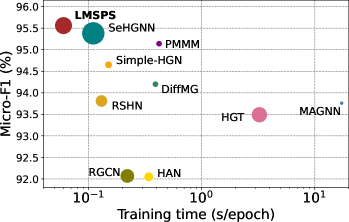
(a) DBLP

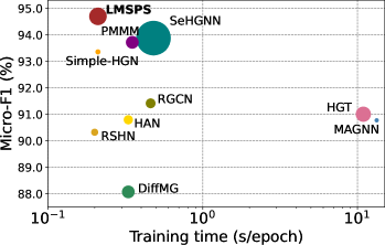
(b) ACM

Figure 4: Micro-F1 scores, time consumption, and parameters of various HGNNs on DBLP and ACM. GTN has a large time consumption and parameters. We ignore it for ease of illustration.

D.3 Effectiveness of the Search Algorithm

This subsection explores the effectiveness of the search algorithm. In our architecture, our meta-paths are replaced by those meta-paths discovered by other methods. DARTS (Liu et al., 2019a) is the first differentiable search algorithm in neural networks. SPOS (Guo et al., 2020) is a classic singe-path differentiable algorithm. DARTS and SPOS aim to search operations, like $3\times 3$ convolution, in convolutional neural networks. DiffMG (Ding et al., 2021) and PMMM (Li et al., 2023) search for meta-graphs instead of meta-paths and cannot search on large-scale datasets. We ignore these differences and focus on the algorithms. The derivation strategies of the four methods are unsuitable for discovering multiple meta-paths. So we changed their derivation strategies to ours to improve their performance. We report the Micro-F1 scores of DBLP, IMDB, and ACM in Table 9. It can be seen that LMSPS shows the best performance, verifying the effectiveness of our search algorithm.

D.4 Comparison on Training Efficiency

We show the time cost and parameters of LMSPS and the advanced baselines on DBLP and ACM in Figure 4. Following the convention (Lv et al., 2021; Yang et al., 2023), we measure the average time consumption of one epoch for each model. The area of the circles represents the parameters. The hidden size is set to $512$ and the maximum hop or layer is $6$ for DBLP and $5$ for ACM for all methods to test the training time and parameters under the same setting. Some methods perform quite poorly under the large maximum hop or layer. So we show the performance from Table 3 of the main text, which is the results under their best settings. Figure 4 shows that LMSPS has advantages in both training efficiency and performance. Our searched meta-paths are universal after searching once and can be applied to other meta-path-based HGNNs based on Table 6. Because other meta-path-based HGNNs don’t include the time for discovering manual meta-paths, we also exclude our search time for discovering meta-paths in Figure 4. The search time is shown in Figure 3 (c) of the main text.

Table 10: Micro-F1 ($\%$) of LMSPS and baselines on Freebase.

Method	Freebase
RSHN (Zhu et al., 2019)	$OOM$
HetSANN (Hong et al., 2020)	$OOM$
GTN (Yun et al., 2019)	$OOM$
HGT (Hu et al., 2020b)	$60.51\pm 1.16$
Simple-HGN (Lv et al., 2021)	$66.29\pm 0.45$
HINormer (Mao et al., 2023)	$-$
RGCN (Schlichtkrull et al., 2018)	$58.33\pm 1.57$
HetGNN (Zhang et al., 2019)	$OOM$
HAN (Wang et al., 2019)	$54.77\pm 1.40$
MAGNN (Fu et al., 2020)	$OOM$
SeHGNN (Yang et al., 2023)	$63.41\pm 0.47$
DiffMG (Ding et al., 2021)	$-$
PMMM (Li et al., 2023)	$-$
LMSPS	$66.52\pm 0.49$

D.5 Further Comparison on Freebase Dataset

Compared with DBLP, IMDB, and ACM, Freebase is less employed by recent HGNNs due to the appearance of ogbn-mag. We ignore Freebase in the main text because of the space limitation. Here, we compare LMSPS with the related baselines on Freebase from HGB (Lv et al., 2021) in Table 10 using the settings in Sections 6.2 and Appendix D.2. As we can see, LMSPS outperforms other HGNNs on Freebase, which is consistent with the results in Table 3.

Table 11: Experiments on DBLP, IMDB, ACM, and ogbn-mag to analyze the effects of different blocks in LMSPS. PS means progressive sampling strategy, and SE means sampling evaluation strategy. * means replacing the concatenation operation with the transformer module, and $\dagger$ means employing all meta-paths and transformer module.

Method	DBLP	IMDB	ACM	ogbn-mag
LMSPS	$95.66\pm 0.20$	$68.70\pm 0.26$	$94.69\pm 0.36$	$54.83\pm 0.20$
LMSPS w/o PS	$95.00\pm 0.19$	$66.52\pm 0.37$	$93.14\pm 0.41$	$47.66\pm 0.45$
LMSPS w/o SE	$95.48\pm 0.24$	$67.13\pm 0.47$	$94.15\pm 0.31$	$52.94\pm 0.34$
LMSPS *	$95.57\pm 0.23$	$68.54\pm 0.16$	$94.63\pm 0.28$	$54.72\pm 0.42$
LMSPS †	$95.38\pm 0.21$	$68.58\pm 0.34$	$94.57\pm 0.39$	$OOM$

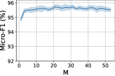
(a) DBLP

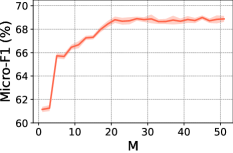
(b) IMDB

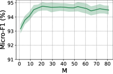
(c) ACM

Figure 5: Micro-F1 with respect to different hyper-parameter $M$ on DBLP, IMDB, and ACM.

D.6 Ablation Study

Two components differentiate our LMSPS from other HGNNs: search algorithm and semantic fusion without attention. The search algorithm consists of a progressive sampling algorithm and a sampling evaluation strategy. Additionally, many HGNNs (Hu et al., 2020b; Yang et al., 2023; Mao et al., 2023) employ the attention mechanism to fuse semantic information. In LMSPS, the difference of importance between the searched effective meta-paths is much smaller than that between the full meta-path set, making the attention mechanism seem unnecessary. We explore how each of them improves performance through ablation studies on DBLP, IMDB, ACM, and ogbn-mag under maximum hops $6$, $5$, $5$, $6$, respectively. As shown in Table 11, the performance of LMSPS significantly decreases when removing progressive sampling or sampling evaluation strategy. Using a transformer block for semantic attention on searched meta-paths can not improve performance, indicating semantic attention is not necessary for LMSPS. In addition, employing a transformer block for semantic attention on all meta-paths shows slightly worse performance, even if using many more meta-paths, indicating that the transformer can’t eliminate the negative effects of noise. It is reasonable because attention values are calculated based on softmax and are positive even for noise. It can explain why transformer-based methods like HGT (Hu et al., 2020b) don’t work well on obgn-mag,

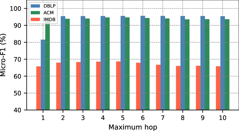
Figure 6: Micro-F1 scores with respect to different maximum hops on DBLP, IMDB, and ACM.

D.7 Hyperparameter Study

LMSPS randomly samples $M$ meta-paths at each epoch in the search stage and selects the top-$M$ meta-paths in the training stage. Here, we perform analysis on hyper-parameter $M$ on DBLP, IMDB, and ACM. As illustrated in Figure 5, the performance of LMSPS increases with the growth of $M$ when $M$ is small. In addition, the performance on DBLP and ACM slightly decreases when $M$ is larger than a certain threshold, indicating excessive meta-paths don’t benefit performance for some datasets. For unity, we set $M=30$ for all datasets.

To observe the impact of different maximum hop values, we show the Micro-F1 of LMSPS with respect to different maximum hop values on DBLP, IMDB, and ACM in Figure 6. We can see LMSPS show the best performance when the maximum hop is $5$ or $6$. Additionally, the performance of LMSPS does not always increase with the value of the maximum hop, and the best maximum hop depends on the dataset.

Appendix E Reproducibility Statement

We have provided the motivation for dataset selection and listed hyper-parameters used for the experiments. All reported results are the average of multiple experiments with standard deviations. We have included a pseudocode description of our method in Appendix B, and describe raining details in Section 6.2 and Appendix D.2. The source code has been submitted as supplementary materials with clear commands on reproducing our results.

Appendix F Limitations

It is noteworthy that the performance of LMSPS does not always increase with the value of the maximum hop. For instance, based on Figure 3 (a), LMSPS can effectively utilize 12-hop meta-paths on DBLP with high performance and low cost. However, the optimal performance for LMSPS is observed when the maximum hop is $6$. It can be attributed to the constraint of maintaining constant time complexity by setting the number of searched meta-paths to $30$ for different maximum hop values. When the maximum hop value is $12$, the number of target-node-related meta-paths exceeds $1400$ (Figure 3 (a)). Searching for $30$ effective meta-paths from such an extensive search space is notably challenging, despite LMSPS being the most effective method for meta-path search (as indicated in Table 9). The advantages of utilizing longer meta-path confers fall short of compensating for the associated drawbacks of much more challenging search space. So, the best maximum hop depends on the dataset and task and cannot be determined automatically.

Nevertheless, based on Table 1, the time complexity of LMSPS does not increase with the maximum hop. Consequently, it provides an effective solution for utilizing long-range dependency on heterogeneous graphs for possible applications on sparser real-world datasets. In Table 4, we conduct experiments on four constructed datasets based on ogbn-mag to demonstrate that the advantages of utilizing long-range dependencies are more obvious for sparser large-scale heterogeneous graphs. For the constructed datasets, we carefully avoid inappropriate preference seed settings of randomly removing by limiting the maximum in-degree related to edge type. We expect sparser large-scale real heterogeneous datasets or more suitable tasks requiring long-range dependency to emerge in the future so we can fully explore our method.

References

- Alon & Yahav (2021) Alon, U. and Yahav, E. On the bottleneck of graph neural networks and its practical implications. In 9th International Conference on Learning Representations, ICLR, 2021.
- Anandalingam & Friesz (1992) Anandalingam, G. and Friesz, T. L. Hierarchical Optimization: An Introduction. Annals of Operations Research, pp. 1–11, 1992.
- Bianchi et al. (2020) Bianchi, F. M., Grattarola, D., and Alippi, C. Spectral clustering with graph neural networks for graph pooling. In International conference on machine learning, ICML, pp. 874–883. PMLR, 2020.
- Chang et al. (2022) Chang, Y., Chen, C., Hu, W., Zheng, Z., Zhou, X., and Chen, S. MEGNN: Meta-path Extracted Graph Neural Network for Heterogeneous Graph Representation Learning. Knowledge-Based Systems, pp. 107611, 2022.
- Chiang et al. (2019) Chiang, W., Liu, X., Si, S., Li, Y., Bengio, S., and Hsieh, C. Cluster-GCN: An Efficient Algorithm for Training Deep and Large Graph Convolutional Networks. In KDD ’19: In Proceedings of the 25th ACM SIGKDD Conference on Knowledge Discovery and Data Mining, pp. 257–266, 2019.
- Colson et al. (2007) Colson, B., Marcotte, P., and Savard, G. An Overview of Bilevel Optimization. Annals of Operations Research, pp. 235–256, 2007.
- Ding et al. (2021) Ding, Y., Yao, Q., Zhao, H., and Zhang, T. DiffMG: Differentiable Meta Graph Search for Heterogeneous Graph Neural Networks. In KDD ’21: In Proceedings of the 27th ACM SIGKDD Conference on Knowledge Discovery and Data Mining, pp. 279–288, 2021.
- Dong & Yang (2019) Dong, X. and Yang, Y. Searching for a robust neural architecture in four gpu hours. In Proceedings of the IEEE/CVF Conference on Computer Vision and Pattern Recognition, ICCV, pp. 1761–1770, 2019.
- Erridge (2006) Erridge, P. The pareto principle. British Dental Journal, 201(7):419–419, 2006.
- Fu et al. (2020) Fu, X., Zhang, J., Meng, Z., and King, I. MAGNN: Metapath Aggregated Graph Neural Network for Heterogeneous Graph Embedding. In Proceedings of the ACM Web Conference, WWW, pp. 2331–2341, 2020.
- Glorot & Bengio (2010) Glorot, X. and Bengio, Y. Understanding the Difficulty of Training Deep Feedforward Neural Networks. In Proceedings of the Thirteenth International Conference on Artificial Intelligence and Statistics, AISTATS, pp. 249–256, 2010.
- Guo et al. (2020) Guo, Z., Zhang, X., Mu, H., Heng, W., Liu, Z., Wei, Y., and Sun, J. Single Path One-Shot Neural Architecture Search with Uniform Sampling. In European Conference on Computer Vision, ECCV, pp. 544–560, 2020.
- Hamilton et al. (2017) Hamilton, W., Ying, Z., and Leskovec, J. Inductive representation learning on large graphs. Advances in neural information processing systems, NeurIPS, 30, 2017.
- Han et al. (2020) Han, Z., Xu, F., Shi, J., Shang, Y., Ma, H., Hui, P., and Li, Y. Genetic Meta-Structure Search for Recommendation on Heterogeneous Information Network. In CIKM ’20: The 29th ACM International Conference on Information and Knowledge Management, pp. 455–464, 2020.
- He et al. (2023) He, X., Hooi, B., Laurent, T., Perold, A., LeCun, Y., and Bresson, X. A generalization of vit/mlp-mixer to graphs. In International conference on machine learning, ICML, pp. 12724–12745. PMLR, 2023.
- Hong et al. (2020) Hong, H., Guo, H., Lin, Y., Yang, X., Li, Z., and Ye, J. An Attention-based Graph Neural Network for Heterogeneous Structural Learning. In Proceedings of the AAAI Conference on Artificial Intelligence, AAAI, pp. 4132–4139, 2020.
- Hu et al. (2020a) Hu, W., Fey, M., Zitnik, M., Dong, Y., Ren, H., Liu, B., Catasta, M., and Leskovec, J. Open graph benchmark: Datasets for machine learning on graphs. Advances in Neural Information Processing Systems, NeurIPS, 33:22118–22133, 2020a.
- Hu et al. (2021) Hu, W., Fey, M., Ren, H., Nakata, M., Dong, Y., and Leskovec, J. OGB-LSC: A Large-Scale Challenge for Machine Learning on Graphs. In Proceedings of the Neural Information Processing Systems Track on Datasets and Benchmarks, 2021.
- Hu et al. (2020b) Hu, Z., Dong, Y., Wang, K., and Sun, Y. Heterogeneous Graph Transformer. In Proceedings of the ACM Web Conference, WWW, pp. 2704–2710, 2020b.
- Ji et al. (2021) Ji, H., Wang, X., Shi, C., Wang, B., and Philip, S. Y. Heterogeneous Graph Propagation Network. IEEE Transactions on Knowledge and Data Engineering, pp. 521–532, 2021.
- Keriven (2022) Keriven, N. Not too little, not too much: a theoretical analysis of graph (over) smoothing. Advances in Neural Information Processing Systems, NeurIPS, 35:2268–2281, 2022.
- Kingma & Ba (2015) Kingma, D. P. and Ba, J. Adam: A Method for Stochastic Optimization. In Bengio, Y. and LeCun, Y. (eds.), International Conference on Learning Representations, ICLR, 2015.
- Li et al. (2023) Li, C., Xu, H., and He, K. Differentiable Meta Multigraph Search with Partial Message Propagation on Heterogeneous Information Networks. Proceedings of the AAAI Conference on Artificial Intelligence, AAAI, 2023.
- Li et al. (2019) Li, G., Muller, M., Thabet, A., and Ghanem, B. Deepgcns: Can gcns go as deep as cnns? In Proceedings of the IEEE/CVF international conference on computer vision, ICCV, pp. 9267–9276, 2019.
- Li et al. (2021a) Li, J., Peng, H., Cao, Y., Dou, Y., Zhang, H., Philip, S. Y., and He, L. Higher-order Attribute-enhancing Heterogeneous Graph Neural Networks. IEEE Transactions on Knowledge and Data Engineering, pp. 560–574, 2021a.
- Li et al. (2018) Li, Q., Han, Z., and Wu, X.-M. Deeper Insights Into Graph Convolutional Networks for Semi-supervised Learning. In Proceedings of the AAAI conference on artificial intelligence, AAAI, 2018.
- Li et al. (2021b) Li, Y., Jin, Y., Song, G., Zhu, Z., Shi, C., and Wang, Y. GraphMSE: Efficient Meta-path Selection in Semantically Aligned Feature Space for Graph Neural Networks. In Proceedings of the AAAI Conference on Artificial Intelligence, AAAI, pp. 4206–4214, 2021b.
- Liu et al. (2019a) Liu, H., Simonyan, K., and Yang, Y. DARTS: differentiable architecture search. In 7th International Conference on Learning Representations, ICLR, 2019a.
- Liu et al. (2019b) Liu, H., Simonyan, K., and Yang, Y. DARTS: Architecture Search. In 7th International Conference on Learning Representations, ICLR, 2019b.
- Lv et al. (2021) Lv, Q., Ding, M., Liu, Q., Chen, Y., Feng, W., He, S., Zhou, C., Jiang, J., Dong, Y., and Tang, J. Are We Really Making Much Progress? Revisiting, Benchmarking and Refining Heterogeneous Graph Neural Networks. In KDD ’21: In Proceedings of the 27th ACM SIGKDD Conference on Knowledge Discovery and Data Mining, pp. 1150–1160, 2021.
- Maddison et al. (2016) Maddison, C. J., Mnih, A., and Teh, Y. W. The concrete distribution: A continuous relaxation of discrete random variables. arXiv preprint arXiv:1611.00712, 2016.
- Mao et al. (2023) Mao, Q., Liu, Z., Liu, C., and Sun, J. Hinormer: Representation learning on heterogeneous information networks with graph transformer. In Proceedings of the ACM Web Conference, WWW, pp. 599–610, 2023.
- Ning et al. (2022) Ning, W., Cheng, R., Shen, J., Haldar, N. A. H., Kao, B., Yan, X., Huo, N., Lam, W. K., Li, T., and Tang, B. Automatic meta-path discovery for effective graph-based recommendation. In Proceedings of the 31st ACM International Conference on Information & Knowledge Management, pp. 1563–1572, 2022.
- Paszke et al. (2019) Paszke, A., Gross, S., Massa, F., Lerer, A., Bradbury, J., Chanan, G., Killeen, T., Lin, Z., Gimelshein, N., Antiga, L., et al. Pytorch: An imperative style, high-performance deep learning library. Advances in Neural Information Processing Systems, NeurIPS, 32, 2019.
- Real et al. (2017) Real, E., Moore, S., Selle, A., Saxena, S., Suematsu, Y. L., Tan, J., Le, Q. V., and Kurakin, A. Large-scale evolution of image classifiers. In International conference on machine learning, ICML, pp. 2902–2911, 2017.
- Sanders (1987) Sanders, R. The pareto principle: its use and abuse. Journal of Services Marketing, 1(2):37–40, 1987.
- Schlichtkrull et al. (2018) Schlichtkrull, M., Kipf, T. N., Bloem, P., Berg, R. v. d., Titov, I., and Welling, M. Modeling Relational Data with Graph Convolutional Networks. In European semantic web conference, pp. 593–607, 2018.
- Shi et al. (2021) Shi, Y., Huang, Z., Feng, S., Zhong, H., Wang, W., and Sun, Y. Masked Label Prediction: Unified Message Passing Model for Semi-supervised Classification. In Proceedings of the Thirtieth International Joint Conference on Artificial Intelligence, IJCAI, pp. 1548–1554, 2021.
- Sun et al. (2021) Sun, C., Gu, H., and Hu, J. Scalable and Adaptive Graph Neural Networks with Self-label-enhanced Training. arXiv preprint arXiv:2104.09376, 2021.
- Sun et al. (2020) Sun, K., Lin, Z., and Zhu, Z. Multi-stage Self-supervised Learning for Graph Convolutional Networks on Graphs with Few Labeled Nodes. In Proceedings of the AAAI Conference on Artificial Intelligence, AAAI, pp. 5892–5899, 2020.
- Sun & Han (2012) Sun, Y. and Han, J. Mining Heterogeneous Information Networks: A Structural Analysis Approach. SIGKDD Explor., pp. 20–28, 2012.
- Sun et al. (2011) Sun, Y., Han, J., Yan, X., Yu, P. S., and Wu, T. PathSim: Meta Path-Based Top-K Similarity Search in Heterogeneous Information Networks. Proc. VLDB Endow., pp. 992–1003, 2011.
- Tolstikhin et al. (2021) Tolstikhin, I. O., Houlsby, N., Kolesnikov, A., Beyer, L., Zhai, X., Unterthiner, T., Yung, J., Steiner, A., Keysers, D., Uszkoreit, J., et al. Mlp-mixer: An all-mlp architecture for vision. Advances in Neural Information Processing Systems, NeurIPS, 34:24261–24272, 2021.
- Wang & Leskovec (2020) Wang, H. and Leskovec, J. Unifying Graph Convolutional Neural Networks and Label Propagation. arXiv preprint arXiv:2002.06755, 2020.
- Wang et al. (2021) Wang, R., Cheng, M., Chen, X., Tang, X., and Hsieh, C.-J. Rethinking architecture selection in differentiable nas. In International Conference on Learning Representation, ICLR, 2021.
- Wang et al. (2019) Wang, X., Ji, H., Shi, C., Wang, B., Ye, Y., Cui, P., and Yu, P. S. Heterogeneous Graph Attention Network. In Proceedings of the ACM Web Conference, WWW, pp. 2022–2032, 2019.
- Wang et al. (2022) Wang, Z., Jiang, W., Zhu, Y. M., Yuan, L., Song, Y., and Liu, W. Dynamixer: a vision mlp architecture with dynamic mixing. In International conference on machine learning, ICML, pp. 22691–22701. PMLR, 2022.
- Xie & Yuille (2017) Xie, L. and Yuille, A. L. Genetic CNN. In IEEE International Conference on Computer Vision, ICCV, pp. 1388–1397, 2017.
- Xie et al. (2019) Xie, S., Zheng, H., Liu, C., and Lin, L. SNAS: Stochastic Neural Architecture Search. In 7th International Conference on Learning Representations, ICLR, 2019.
- Xue et al. (2021) Xue, C., Wang, X., Yan, J., Hu, Y., Yang, X., and Sun, K. Rethinking Bi-Level Optimization in Neural Architecture Search: A Gibbs Sampling Perspective. In Proceedings of the AAAI Conference on Artificial Intelligence, AAAI, pp. 10551–10559, 2021.
- Yang et al. (2023) Yang, X., Yan, M., Pan, S., Ye, X., and Fan, D. Simple and Efficient Heterogeneous Graph Neural Network. Proceedings of the AAAI Conference on Artificial Intelligence, AAAI, 2023.
- Yao et al. (2020) Yao, Q., Xu, J., Tu, W.-W., and Zhu, Z. Efficient Neural Architecture Search via Proximal Iterations. In Proceedings of the AAAI Conference on Artificial Intelligence, AAAI, 2020.
- Ying et al. (2021) Ying, C., Cai, T., Luo, S., Zheng, S., Ke, G., He, D., Shen, Y., and Liu, T.-Y. Do transformers really perform badly for graph representation? Advances in Neural Information Processing Systems, NeurIPS, 34:28877–28888, 2021.
- Yu et al. (2020) Yu, L., Shen, J., Li, J., and Lerer, A. Scalable Graph Neural Networks for Heterogeneous Graphs. arXiv preprint arXiv:2011.09679, 2020.
- Yun et al. (2019) Yun, S., Jeong, M., Kim, R., Kang, J., and Kim, H. J. Graph Transformer Networks. In Advances in Neural Information Processing Systems, NeurIPS, pp. 11960–11970, 2019.
- Zhang et al. (2019) Zhang, C., Song, D., Huang, C., Swami, A., and Chawla, N. V. Heterogeneous Graph Neural Network. In KDD ’19: In Proceedings of the 25th ACM SIGKDD Conference on Knowledge Discovery and Data Mining, pp. 793–803, 2019.
- Zhang et al. (2022) Zhang, W., Yin, Z., Sheng, Z., Li, Y., Ouyang, W., Li, X., Tao, Y., Yang, Z., and Cui, B. Graph Attention Multi-layer Perceptron. In KDD ’22: In Proceedings of the 28th ACM SIGKDD Conference on Knowledge Discovery and Data Mining, pp. 4560–4570, 2022.
- Zhong et al. (2020) Zhong, Z., Li, C.-T., and Pang, J. Reinforcement learning enhanced heterogeneous graph neural network. arXiv preprint arXiv:2010.13735, 2020.
- Zhu et al. (2019) Zhu, S., Zhou, C., Pan, S., Zhu, X., and Wang, B. Relation Structure-aware Heterogeneous Graph Neural Network. In 2019 IEEE International Conference on Data Mining, ICDM, pp. 1534–1539, 2019.