Information decomposition to identify relevant variation in complex systems
with machine learning

Abstract

One of the fundamental steps toward understanding a complex system is identifying variation at the scale of the system’s components that is most relevant to behavior on a macroscopic scale. Mutual information is a natural means of linking variation across scales of a system due to its independence of the particular functional relationship between variables. However, estimating mutual information given high-dimensional, continuous-valued data is notoriously difficult, and the desideratum—to reveal important variation in a comprehensible manner—is only readily achieved through exhaustive search. Here we propose a practical, efficient, and broadly applicable methodology to decompose the information contained in a set of measurements by lossily compressing each measurement with machine learning. Guided by the distributed information bottleneck as a learning objective, the information decomposition sorts variation in the measurements of the system state by relevance to specified macroscale behavior, revealing the most important subsets of measurements for different amounts of predictive information. Additional granularity is achieved by inspection of the learned compression schemes: the variation transmitted during compression is composed of distinctions among measurement values that are most relevant to the macroscale behavior. We focus our analysis on two paradigmatic complex systems: a Boolean circuit and an amorphous material undergoing plastic deformation. In both examples, specific bits of entropy are identified out of the high entropy of the system state as most related to macroscale behavior for insight about the connection between micro- and macro- in the complex system. The identification of meaningful variation in data, with the full generality brought by information theory, is made practical for the study of complex systems.

A complex system is a system of interacting components where some sense of order present at the scale of the system is not apparent, or even conceivable, from the observations of single components [1, 2]. A broad categorization, it includes many systems of relevance to our daily lives, from the economy to the internet and from the human brain to artificial neural networks [3, 4]. Before attempting a reductionist description of a complex system, one must first identify variation in the system that is most relevant to emergent order at larger scales. The notion of relevance can be formalized with information theory, wherein mutual information serves as a general measure of statistical dependence to connect variation across different scales of system behavior [5, 6]. Information theory and complexity science have a rich history; information theory commonly forms the foundation of definitions of what it means to be complex [7, 8, 9, 10].

Machine learning is well-suited for the analysis of complex systems, grounded in its natural capacity to identify patterns in high dimensional data [11]. However, distilling insight from a successfully trained model is often infeasible due to a characteristic lack of interpretability of machine learning models [12, 13]. Restricting to simpler classes of models, for example linear combinations of observables, recovers a degree of interpretability at the expense of functional expressivity [14]. For the study of complex systems, such a trade-off is unacceptable if the complexity of the system is no longer faithfully represented. In this work, we do not attempt to explain the relationship between microscale and macroscale, and are instead interested in identifying the information contained in microscale observables that is most predictive of macroscale behavior—independent of functional relationship.

We employ a recent method from interpretable machine learning that identifies the most relevant information in a set of measurements [15]. Based on the distributed information bottleneck [16, 17], a variant of the information bottleneck (IB) [18], the method lossily compresses a set of measurements while preserving information about a relevance quantity. Optimization serves to decompose the information present in the measurements, providing a general-purpose method to identify the important variation in composite measurements of complex systems.

Identifying important variation is a powerful means of analysis of complex systems, as we demonstrate on two paradigmatic examples. First we study a Boolean circuit, whose fully-specified joint distribution and intuitive interactions between variables facilitate understanding of the information decomposition found by the distributed IB. Boolean circuits are networks of binary variables that interact through logic functions, serving as the building blocks of computation [19] and as elementary models of gene control networks [20, 21]. Second, we decompose the information contained in the local structure of an amorphous material subjected to global deformation. Amorphous materials are condensed matter systems composed of simple elements (e.g., atoms or grains) that interact via volume exclusion and whose disorder gives rise to a host of complex macroscale phenomena, such as collective rearrangement events spanning a wide range of magnitudes [22, 23] and nontrivial phase transitions [24, 25, 26, 27]. Although the state space that describes all of the degrees of freedom is large, as is generally true of complex systems, the proposed method is able to identify important bits of variation by partitioning entropy and leveraging machine learning to process the high dimensional data.

I Methods

Mutual information is a measure of statistical dependence between two random variables $X$ and $Y$ that is independent of the functional transformation that relates $X$ and $Y$ (in contrast to linear correlation, for example, which measures the degree to which two variables are linearly related). Mutual information is defined as the entropy reduction in one variable after learning the value of the other [28],

$$I(X;Y)=H(Y)-H(Y|X),$$ (1)

with $H(X)=\mathbb{E}_{x\sim p(x)}[-\textnormal{log}\ p(x)]$ Shannon’s entropy [29].

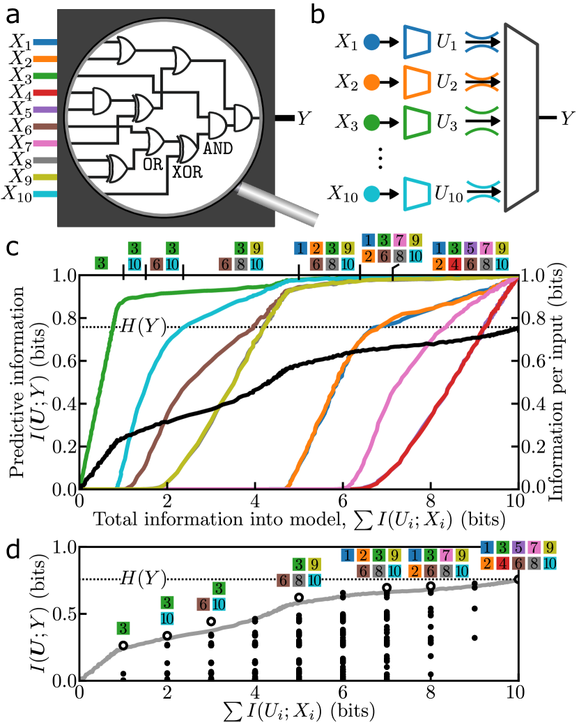
Figure 1: Decomposing the information contained in the inputs of a Boolean circuit. (a) Ten binary inputs $\bm{X}=(X_{1},...,X_{10})$ are connected via AND, OR, and XOR gates to a binary output $Y$. (b) A lossy compression $U_{i}$ is learned for each $X_{i}$ and then all $U_{i}$ are combined as input to a machine learning model trained to predict $Y$. (c) The distributed information plane displays the predictive information about the output (left vertical axis, black) as a function of the total information utilized about the input. For each value of total information into the model there is an allocation of information to the input gates indicating their relevance to the output $Y$ (right vertical axis, colors corresponding to input gates in panel (a)). The subset of inputs identified as containing the most relevant information ($I(U_{i};X_{i})\geq 0.1$ bits) are indicated at the top of the plot. (d) The mutual information between all subsets of input channels and $Y$ are displayed on the distributed information plane as black circles. The optimization of the distributed IB (gray curve) identified subsets of inputs that contain the most predictive information (open circles).

The distributed information bottleneck is an optimization objective to extract the information most relevant to a variable $Y$ from a composite measurement: a random vector $\bm{X}=(X_{1},...,X_{N})$ [16, 30, 15]. Each component $X_{i}$ undergoes lossy compression to an auxiliary variable $U_{i}=f(X_{i})$, and then the compressed variables $\bm{U}=(U_{1},...,U_{N})$ are used to predict the output $Y$. Minimization of the distributed IB Lagrangian,

$$\mathcal{L}_{\textnormal{DIB}}=\beta\sum_{i=1}^{N}I(U_{i};X_{i})-I(\bm{U};Y),$$ (2)

extracts the entropy (or information) in $\bm{X}$ that is most descriptive of $Y$. By sweeping over the magnitude of the bottleneck strength $\beta$, a continuous spectrum of approximations to the relationship between $\bm{X}$ and $Y$ is found. The optimized compression schemes for each component of $\bm{X}$ reveal the amount of relevant information and the specific entropy selected for every level of approximation.

In place of Eqn. 2, variational bounds on mutual information have been developed that are amenable to data and machine learning [31, 17]. The lossy compression schemes are parameterized by neural networks that encode data points to probability distributions in a continuous latent space. Transmitted information is upper bounded by the expectation of the Kullback-Leibler divergence [28] between the encoded distributions and an arbitrary prior distribution, identical to the process of information restriction in a variational autoencoder [32, 31]. Over the course of training, the amount of information conveyed by each compression scheme $I(U_{i};X_{i})$ is estimated using bounds derived in Ref. [33]. Although mutual information is generally difficult to estimate from data [34], compressing the partial measurements $X_{i}$ separately isolates the information such that the amount of mutual information is small enough to allow precise estimates, with the interval between bounds on the order of 0.01 bits. Details about mutual information estimation are in Appendix A.

II Results

Boolean circuit. A Boolean circuit (Fig. 1a) was constructed with ten binary inputs $\bm{X}=(X_{1},...,X_{10})$ and a binary output $Y$. Assuming a uniform distribution over inputs, the truth table specifies the joint distribution $p(x_{1},...,x_{10},y)$, and the interactions between inputs are prescribed by a wiring of logical AND, OR, and XOR gates. An information bottleneck was distributed to every input $X_{i}$ to monitor from where the predictive information originated via compressed variables $U_{i}$ (Fig. 1b). We trained a multilayer perceptron (MLP) to learn the relationship between the lossy compressions $\bm{U}$ and $Y$.

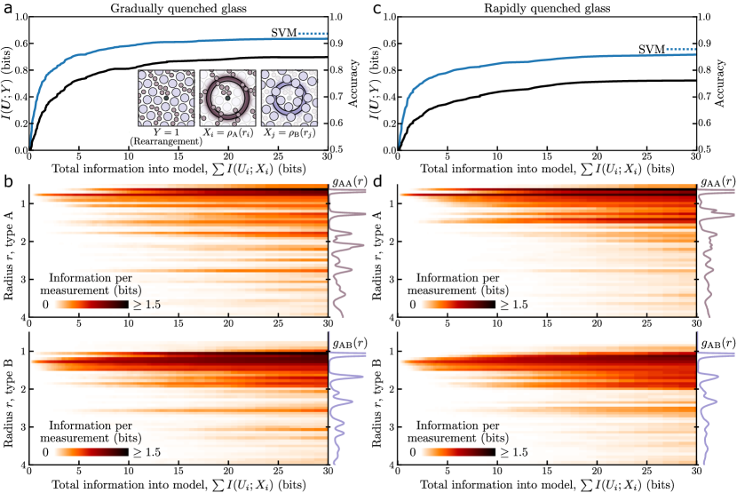
Figure 2: Decomposing structural information about imminent rearrangement in a sheared glass. (a) Inset: Given a local neighborhood in a sheared glass, fifty densities each of radial shells for the small (type A) and large (type B) particles were used to predict whether the neighborhood is the locus of an imminent rearrangement event. Main: For a gradually quenched glass, the information that is predictive of rearrangement (black) increased as the most predictive density information was identified and incorporated into the machine learning model. The accuracy (blue) was comparable to a support vector machine (SVM) (dashed line) after around twenty bits. (b) Sharing the horizontal axis with panel (a), the amount of information extracted about each of the radial density measurements of small (top) and large (bottom) particles reveals the radii with the most predictive information at each level of approximation. The system’s average density values for each particle type with type A at the center, also known as the radial distribution functions $g_{\textnormal{AA}}(r)$ and $g_{\textnormal{AB}}(r)$, are shown on the right. (c,d) The same as panels (a, b) but for glass that was prepared via a rapid quench rather than a gradual quench.

Over the course of a single training run, the coefficient of the information bottleneck strength $\beta$ was swept to obtain a spectrum of predictive models. The distributed information plane (Fig. 1c) [15] displays the predictive power as a function of the total information about the inputs $\sum I(U_{i};X_{i})$. The predictive performance ranged from zero predictive information without any information about the inputs (Fig. 1c, lower left) to all entropy $H(Y)$ accounted for by utilizing all ten bits of input information (Fig. 1c, upper right). For every point on the spectrum there was an allocation of information over the inputs; the distributed IB objective identified the information across all inputs that was most predictive. The most predictive information about $Y$ was found to reside in $X_{3}$—the input that routes through the fewest gates to $Y$—and then in the pair $X_{3},X_{10}$, and so on.

Powered by machine learning, we traversed the space of lossy compression schemes of $X_{i}$, decomposing the information contained in the circuit inputs about the output. Included in the space of compression schemes is information transmitted about each of the $2^{10}$ discrete subsets of the inputs. To be concrete, there are ten subsets of a single input, 45 pairs of inputs, and so on, with each subset sharing mutual information with $Y$ based on the role of the specific inputs inside the circuit. Fig. 1d displays the information contained in every discrete subset of inputs (black points) along with the continuous trajectory found by optimization of the distributed IB (gray curve). The distributed IB, maximizing predictive information while minimizing information taken from the inputs, closely traced the upper boundary of discrete information allocations and identified a majority of the most informative subsets of inputs. To decompose the information in the circuit’s inputs required only a single sweep with the distributed IB, not an exhaustive search through all subsets of inputs. We note that the product of the distributed IB is not an ordering of single variable mutual information terms $I(X_{i};Y)$, which would be straightforward to calculate, but instead the ordering of information selected from all of $\bm{X}$ that is maximally informative about $Y$.

Decomposing structural information in a physical system. Linking structure and dynamics in amorphous materials—complex systems consisting of particles that interact primarily through volume exclusion—has been a longstanding challenge in physics [35, 36, 37, 38]. Searching for signatures of collective behavior in the multitude of microscopic degrees of freedom is an endeavor emblematic of complex systems more generally and one well-suited for machine learning and information theory. We accept that the functional relationship between the micro- and macroscale variation is potentially incomprehensible, and are instead interested in the information at the microscale that is maximally predictive of behavior at the macroscale. While prior work has analyzed the information content of hand-crafted structural descriptors individually [39, 40, 41], the distributed IB searches through the space of information from many structural measurements in combination.

Two-dimensional simulated glasses, prepared by either rapid or gradual quenching and composed of small (type A) and large (type B) particles that interact with a Lennard-Jones potential, were subjected to global shear deformation [38]. Local regions were identified as the origins of imminent rearrangement and paired with negative samples from elsewhere in the system to create a binary classification dataset.

We first considered a scheme of measurements of the microscale structure that has been associated with plastic rearrangement in a variety of amorphous systems: the densities of radial bands around the center of a region [42, 43]. By training a support vector machine (SVM) to predict rearrangement based on the radial density measurements, a linear combination of the values is learned. In the literature, that combination is commonly referred to as softness, and has proven to be a useful local order parameter [44, 45, 46, 47].

We approached the same prediction task from an information theoretic perspective, seeking the specific bits of variation in the density measurements that are most predictive of collective rearrangement. Each radial density measurement underwent lossy compression by its own neural network before all compressions were concatenated and used as input to an MLP to predict rearrangement. By sweeping $\beta$, a single optimization recovered a sequence of approximations, each allocating a limited amount of information across the 100 density measurements to be most predictive of imminent rearrangement (Fig. 2).

The trajectories in the distributed information plane, for both gradually and rapidly quenched glasses, reflect the growth of predictive information and prediction accuracy given maximally predictive information about the radial densities (Fig. 2a,c). With only one bit of information from the density measurements, 71.8% predictive accuracy was achieved for the gradually quenched glass and 69.5% was achieved for the rapidly quenched glass; with twenty bits, the accuracy jumped to 91.3% and 85.4%, respectively. Beyond twenty bits of density information, the predictive accuracy became comparable to that of the support vector machine, which can utilize all of the continuous-valued density measurements for prediction with a linear relationship.

For every point along the trajectory, information was identified from the density measurements that, together, formed the combination of bits that were most predictive of rearrangement (Fig. 2b,d). The majority of the information was selected from smaller radii (close to the center of the region), which can be expected given the localized nature of rearrangement events [35, 36]. Less intuitive is the information decomposition as it relates to the radial distribution functions $g_{\textnormal{AA}}(r)$ and $g_{\textnormal{AB}}(r)$, the system-averaged radial densities of type A and B particles in regions with a type A particle at the center. For both glasses, the most predictive bits originated in the low density radial bands nearest the center. As more information was incorporated into the prediction, the additional bits came from radial bands that corresponded to particular features of $g_{\textnormal{AA}}(r)$ and $g_{\textnormal{AB}}(r)$. Outside of the first low density trough, the selected information often came from the high density radii of type $A$ particles and the low density radii of type $B$ particles; this trend held true for both glasses. While the information decomposition highlighted similar features in both glasses, the more pronounced structure of selected information out to larger radii for the gradually quenched glass is indicative of its higher structural regularity, which is also seen in the pronounced features of its radial distribution functions $g_{\textnormal{AA}}(r)$ and $g_{\textnormal{AB}}(r)$.

The amount of information utilized from each density measurement was predominantly a single bit or less. Of the ways to compress the infinite entropy of a continuous-valued density to a single bit, what was the specific variation extracted from each density measurement? Through inspection of the learned compression schemes, the extracted information can be further decomposed by the degree of distinctions between density values that were preserved for the predictive model (Fig. 3a) [15]. The single most important bit of information for the gradually quenched glass was a composition of partial bits from multiple density measurements, mostly arising from the first low-density shell of each type of particle (Fig. 3b). For both measurements, the compression scheme acted as a threshold on the range of possible density values: values less than a cutoff $\rho^{\prime}$ were indistinguishable from each other for the purposes of prediction and were partially distinguishable from density values above the cutoff. By examining the distribution of density values in these radial shells, we see that the cutoff values leverage the separability of the density distributions when conditioned on rearrangement.

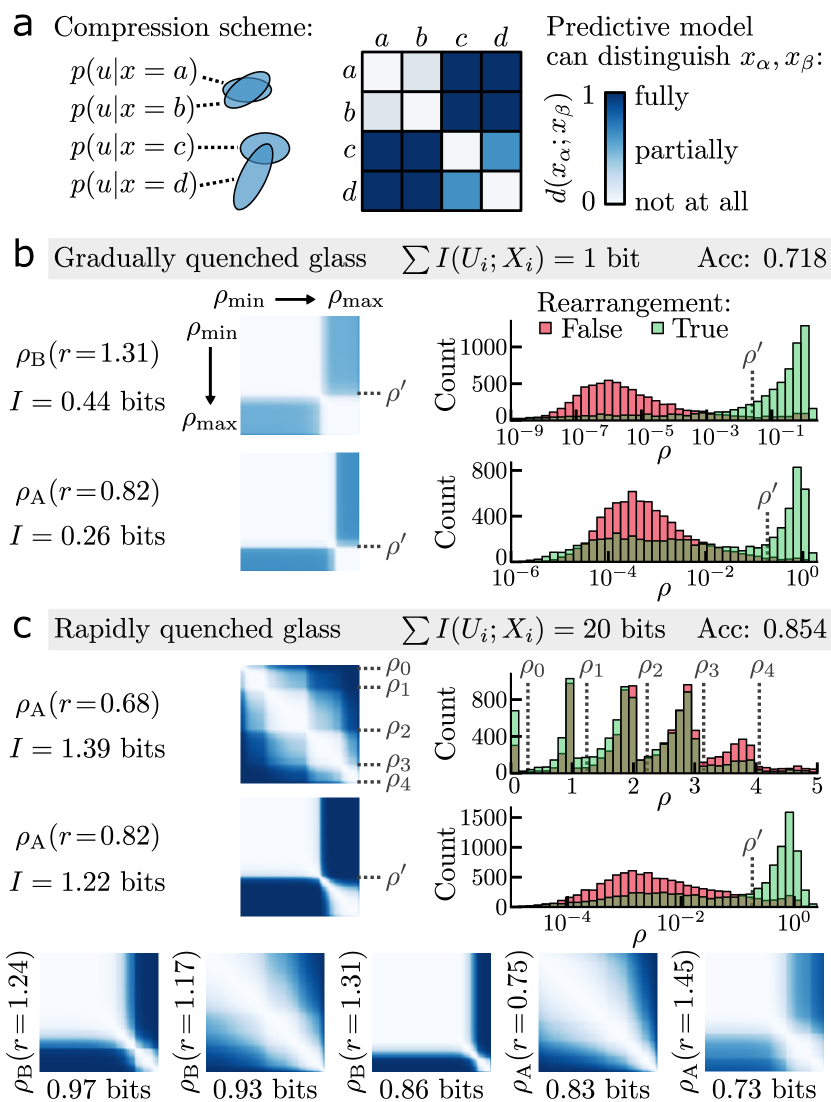
Figure 3: Selected bits of information as distinctions among raw measurement values. (a) Lossy compression is achieved by mapping the raw values of $X$ to probability distributions in latent space. The statistical similarity of the conditional distributions, visualized as a matrix for all pairs of feature values, determines how distinguishable the raw feature values are to the predictive model. (b) The single most predictive bit of information about rearrangement in the gradually quenched glass came predominantly from two density measurements. The distinguishability matrices indicate that the compression scheme applied a simple threshold to these measurements: density values less than a cutoff value $\rho^{\prime}$ were indistinguishable from each other, as were values above the cutoff. The histograms of density values conditioned on rearrangement (right) show that the learned cutoff value separates the probability masses. (c) The twenty most predictive bits of radial density information in the rapidly quenched glass were selected from many radial bands. The two that contribute more than a bit of information each correspond to the density of type $A$ particles near the center; one compression scheme effectively counted the number of particles in the high density shell. The distinguishability matrices of the next five most informative radial bands are shown below.

With more information utilized for prediction, some of the compression schemes differed from simple thresholds (shown for the rapidly quenched glass in Fig. 3c). For the predictive model operating with a total of twenty bits of density information, two density measurements contributed more than a bit each. The learned compression of the first high-density shell of type A particles essentially counted the number of particles in the shell, with distinguishability between densities as if there were several thresholds over the range of the values that act to roughly discretize the density measurement.

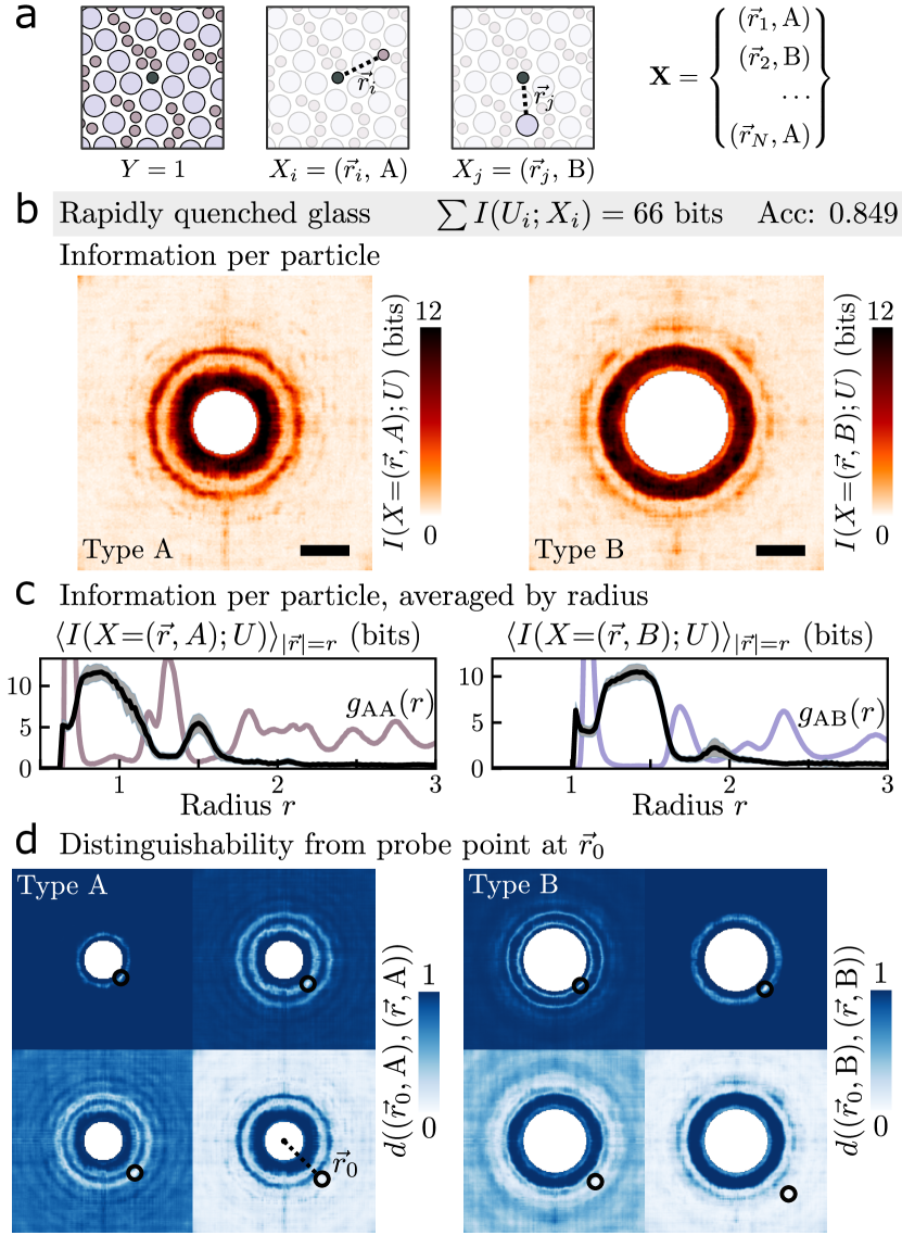
Figure 4: Measuring the positions of all particles. (a) Instead of the density of radial shells, each particle’s position and type in a local neighborhood were used as input measurements to relate to rearrangement. (b) The per-particle information transmitted as a function of particle position, for the small type A (left) and large type B (right) particles, for the predictive model utilizing 66 bits of information about the rapidly quenched glass. The scale bar is a distance of one in simulation units. (c) Averaged radially, the information (black) resides in particles that are situated in the first troughs of the radial distribution function, $g(r)$ (colored curves). (d) For a particle at position $\vec{r}_{0}$, the distinguishability of particles of the same type at all other locations indicates that negligible azimuthal information was transmitted.

Information decomposition with the distributed IB depends upon the particular scheme used to measure the system [48]. In the study of complex systems, there can be multiple ‘natural’ schemes of measuring a system state. Density measurements of radial bands lead to an essentially linear relationship between structure and rearrangement [44]; what if we had not inherited such a fortuitous measurement scheme? Another natural basis of measurements is the position of all of the particles (Fig. 4a). In contrast to radial density measurements, per-particle measurements lack a canonical ordering; accordingly, we used a permutation-invariant transformer architecture for the predictive model [49]. Every particle position was transmitted in parallel through a single compression channel, rather than through a uniquely learned compression scheme per measurement as before. An analogue of the distributed IB task is to write a note for each particle in the region with the goal to predict whether the region will rearrange. Under a constraint on time or effort, more careful notes would be taken for the informative particles, while less careful notes would be taken for the rest.

The per-particle measurement scheme imposed no structure on the selection of configurational information. Nevertheless, we found that the information cost per particle as a function of the position in the neighborhood had a radial structure (Fig. 4b). The information per particle was highest in the low density radial bands near the center of the region (Fig. 4c), and inspection of the compression scheme indicated that negligible azimuthal information was transmitted (Fig. 4d). The information decomposition allowed for similar insights to be derived as in the radial density measurement scheme, even though the nature of the predictive model in the two cases was substantially different. Additionally, because the distributed IB operates entirely on the input side of an arbitrary predictive model, the information analysis was agnostic to whether the model was a simple fully connected network or a more complicated transformer architecture.

III Discussion

A universal challenge faced when studying complex systems, fundamental to what makes a system complex, is the abundance of entropy from the perspective of the microscale that obscures relevant information about macroscale behavior. The generality of mutual information as a measure of statistical relatedness, and the expressivity of deep learning when handling high-dimensional data, allow the distributed IB to be as readily utilized to identify structural defects relevant to a given material property as it is to reveal gene variation relevant to a given affliction. Tens, hundreds, and potentially thousands of measurements of a complex system are handled simultaneously, rendering practical analyses that would have previously been infeasible through exhaustive search or severely limited by constraints on functional relationships between variables.

Information theory has long held appeal for the analysis of complex systems owing to the generality of mutual information [28, 3]. However, the estimation of mutual information from data is fraught with difficulties [34, 50, 33], which have hindered information theoretic analyses of data from complex systems. By distributing information bottlenecks across multiple partial measurements of a complex system, entropy is partitioned to a degree that makes precise estimation of mutual information possible while simultaneously revealing the most important combinations of bits for insight about the system. Machine learning navigates the space of lossy compression schemes for each variable and allows the identification of meaningful variation without consideration of the black box functional relationship found by the predictive model.

Instead of compressing partial measurements in parallel, the information bottleneck [18] extracts the relevant information from one random variable in its entirety about another, and is foundational to many works in representation learning [51, 52]. In the physical sciences, the IB has been used to extract relevant degrees of freedom with a theoretical equivalence to coarse-graining in the renormalization group [53, 54], and to identify useful reaction coordinates in biomolecular reactions [55]. However, the IB has limited capacity to find useful approximations, particularly when the relationship between $X$ and $Y$ is deterministic (or nearly so) [56, 57]. Much of the spectrum of learned approximations is the trivial noisy rendition of a high-fidelity reconstruction [56, 48]. Additionally, compression schemes found by IB are rarely interpretable because the singular bottleneck occurs after processing the complete input, allowing the compression scheme to involve arbitrarily complex relationships between components of the input without penalty. The distribution of information bottlenecks is critical to an interpretable information decomposition, and to accurately estimating the necessary mutual information terms.

A growing body of literature focuses on a fundamentally different route to decompose the information contained in multiple random variables $\{X_{i}\}$ about a relevant random variable $Y$; that alternative route is partial information decomposition (PID) [58, 59]. Although there is no consensus on how to achieve PID in practice, its goal is to account for the mutual information between $\{X_{i}\}$ and $Y$ in terms of subsets of $\{X_{i}\}$, by analogy to set theory [60]. PID allocates information to the input variables in their entirety, whereas the distributed IB selects partial entropy from the input variables in the form of lossy compression schemes, with one scheme per variable. While PID has been proposed as an information theoretic route to study complex systems [61] and quantify complexity [62], the super-exponential growth of PID terms renders the methodology rather impractical. There are $5\times 10^{22}$ PID terms for a Boolean circuit with 8 inputs [58] and the number of terms for the simple 10 input circuit from Fig. 1 is not known [59]. By contrast, the distributed IB offers a pragmatic route to the decomposition of information in a complex system: it is amenable to machine learning and data, and can readily process one hundred (continuous) input variables as in the amorphous plasticity experiments.

IV Acknowledgements

We gratefully acknowledge Sam Dillavou and Zhuowen Yin for helpful discussions and comments on the manuscript, and Sylvain Patinet for the amorphous plasticity data.

V Code availability

The full code base has been released on Github and may be found through the following link: distributed-information-bottleneck.github.io. Every analysis included in this work can be repeated from scratch with the corresponding Google Colab iPython notebook in this directory.

VI Data availability

The train and validation splits of the amorphous plasticity data, consisting of local neighborhoods that were subsequently “measured” as radial densities (Figs. 2,3) or as per-particle descriptors (Fig. 4), can be found through the project page and can be downloaded here. The full dataset with all particle locations before and after all events is available with the permission of the authors of Ref. [38].

VII Appendix A: Mutual information bounds

The full method presented in this work requires us to bound the mutual information for high dimensional data; identifying this bound is notoriously difficult [34, 50]. Fortunately, there are factors in our favor to facilitate optimization with machine learning and the recovery of tight bounds on the information transmitted by the compression channels $U_{i}$.

To optimize the distributed information bottleneck objective (Eqn. 2) requires an upper bound on $I(U_{i};X_{i})$ and a lower bound on $I(\bm{U};Y)$. The (distributed) variational information bottleneck objective [31, 17] upper bounds $I(U_{i};X_{i})$ with the expectation of the Kullback-Leibler (KL) divergence between the encoded distributions $p(u_{i}|x_{i})$ and an arbitrary prior distribution $r(u_{i})$ in latent space,

$$I(U_{i};X_{i})\leq\mathbb{E}_{x_{i}\sim p(x_{i})}[D_{\textnormal{KL}}(p(u_{i}|x_{i})||r(u_{i}))].$$ (3)

Normal distributions are used for both the encoded distribution, $p(u_{i}|x_{i})=\mathcal{N}(\bm{\mu}=f_{\mu}(x_{i}),\bm{\sigma}=f_{\sigma}(x_{i}))$, and the prior, $r(u_{i})=\mathcal{N}(\bm{0},\bm{1})$ so that the KL divergence has a simple analytic form.

Over the course of training, the KL divergence is computed for each channel $U_{i}$, thereby providing a proxy quantity for the amount of information that is contained in the compression scheme. Although the KL divergence can be used for a qualitative sense of information allocation to features [15], it is a rather poor estimate of the mutual information. Because the encoded distributions $p(u_{i}|x_{i})$ have a known form, we can use the noise contrastive estimation (InfoNCE) lower bound and “leave one out” upper bound from Ref. [33] with a large number of samples to obtain tight bounds on the amount of mutual information in the learned compression schemes.

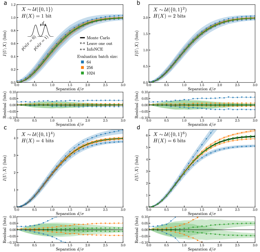
Figure 5: Performance of mutual information bounds. A parameterized compression scheme encodes a discrete $X$ to a separate normal distribution per outcome $x$, each with unit variance in $\mathbb{R}^{32}$ and spaced from the origin by a separation distance $d$. The expectation and standard deviation of the “leave one out” upper and InfoNCE lower bounds are the dashed line and shaded regions, respectively, evaluated over 4096 batches. In the residual plots, which show the difference between the bounds and the Monte Carlo estimate, only the standard deviations for the evaluation batch size of 1024 are displayed. Variables $X$ with (a) one, (b) two, (c) four, and (d) six bits of entropy are used to generate the dataset for evaluation.

The lower and upper bounds on $I(U_{i};X_{i})$ are based on likelihood ratios at points sampled from the dataset $x_{i}\sim p(x_{i})$ and from the corresponding conditional distributions, $u_{i}\sim p(u_{i}|x_{i})$. To be specific, the mutual information for each channel $U=f(X)$ (dropping channel indices for simplicity) is lower bounded by

$$I(U;X)\geq\mathbb{E}\left[\frac{1}{K}\sum_{i}^{K}\log\frac{p(u_{i}|x_{i})}{\frac{1}{K}\sum_{j}^{K}p(u_{i}|x_{j})}\right]$$ (4)

and upper bounded by

$$I(U;X)\leq\mathbb{E}\left[\frac{1}{K}\sum_{i}^{K}\log\frac{p(u_{i}|x_{i})}{\frac{1}{K-1}\sum_{j\neq i}^{K}p(u_{i}|x_{j})}\right].$$ (5)

The expectation values in both equations are taken over samples $\{u_{i},x_{i}\}_{i=1}^{K}$ of size $K$ extracted repeatedly from the joint distribution $p(u,x)=p(x)p(u|x)$. We estimated with as large an evaluation batch size $K$ as feasible given memory and time considerations, and then averaged over multiple batches to reduce the variance of the bound. Evaluation with a batch size of 1024, averaged over 8 draws, yielded bounds on the mutual information that was on the order of 0.01 bits for the Boolean circuit and glass data. The size of the validation dataset for the glass and the size of the truth table of the Boolean circuit were both on the order of one thousand points. Hence, the benefit of averaging comes from repeated sampling of the latent representations.

We show in Fig. 5 the performance of the mutual information bounds for compression schemes that encode up to several bits of information. $X$ is a discrete random variable that is uniformly distributed over its support and has one to six bits of entropy; for each $X$ a fixed dataset of size 1024 was sampled for mutual information estimation according to the following method of compression. Each outcome $x$ was encoded to a normal distribution with unit variance in 32-dimensional space, $p(u|x)=\mathcal{N}(\bm{\mu},\bm{1})$. The encoded distributions were placed along orthogonal axes a distance $d$ from the origin; in the limits of $d=0$ and $d\gg 1$ the information transmitted by the compression scheme is 0 and $H(X)$, respectively.

A Monte Carlo estimate of the mutual information sampled 2$\times$10⁵ points from $p(u,x)$ to compute $\mathbb{E}_{p(u,x)}[\log p(u|x)/p(u)]$. The “leave one out” upper and InfoNCE lower bounds were computed with different evaluation batch sizes $K$, and averaged over 4096 sampled batches. The standard deviation of the bounds is displayed as the shaded region around each trace, and is left out of the plots for the residual (the difference between the bound and the Monte Carlo estimate) for all but the evaluation batch size of 1024.

When the information contained in the compression is less than about two bits—as was the case for the majority of the experiments of the main text—the bounds are tight in expectation for even the smallest evaluation batch size. The variance is reducible by averaging over multiple batches. As the transmitted information grows, the benefit of increasing the evaluation batch size grows more pronounced, though bounds with a range of less than 0.1 bits can still be achieved for up to six bits of transmitted information.

VII.1 Information transmitted per particle

For the per-particle measurement scheme on the amorphous plasticity data, a single compression channel $U$ was used for all particles. The information conveyed by the channel $I(U;X)$ may be estimated as above, with $X$ being the particle position and type. Note that we are particularly interested in the information cost for specific particle positions and for each particle type. The outer summation of the bounds (Eqn. 4 and 5) serves to average over the measurement outcomes $x_{i}$ in a random sample; we use the summand corresponding to $\{x_{i},u_{i}\}$ as the information contribution for the specific outcome $x_{i}$. To generate the information heatmaps of Fig. 4b, we randomly sampled 512 neighborhoods from the dataset, corresponding to an evaluation batch size $K=512\ \textnormal{neighborhoods}\times 50\ \textnormal{particles / neighborhood}=25,600$ particles (data points), and averaged over 100 such batches. A probe particle with specified particle type and position (one for each point in the grid) was inserted into the batch, and then the corresponding summand for the lower and upper information bounds served to quantify the information transmitted per particle. To be specific,

$$I(X=x;U)\geq\mathbb{E}\left[\log\frac{p(u|x)}{\frac{1}{K}\sum_{j}^{K}p(u|x_{j})}\right],$$ (6)

with the expectation taken over $u\sim p(u|x)$ and samples $\{x_{i}\}_{i=1}^{K}\sim\prod_{i}^{K}p(x)$. The upper bound differed only by inclusion of the distribution $p(u|x)$ corresponding to the probe point in the denominator’s sum.

VIII Appendix B: Implementation specifics

All experiments were implemented in TensorFlow and run on a single computer with a 12 GB GeForce RTX 3060 GPU. Computing mutual information bounds repeatedly throughout an optimization run contributed the most to running time. Including the information estimation, the Boolean circuit optimization took about half an hour, and the glass experiments took several hours.

VIII.1 Boolean circuit

Each input may take only one of two values (0 or 1), allowing the encoders to be extremely simple. Trainable scalars $(\vec{\mu}_{i},\textnormal{log}\ \vec{\sigma}_{i}^{2})$ were used to encode $p(u_{i}|x_{i})=\mathcal{N}((2x_{i}-1)\times\vec{\mu}_{i},\vec{\sigma}_{i}^{2})$. The decoder was a multilayer perceptron (MLP) consisting of three fully connected layers with 256 Leaky ReLU units ($\alpha=0.3$) each. We increased the value of $\beta$ logarithmically from $5\times 10^{-4}$ to $5$ in $5\times 10^{4}$ steps, with a batch size of 512 input-output pairs sampled randomly from the entire 1024-element truth table. The Adam optimizer was used with a learning rate of $10^{-3}$.

VIII.2 Amorphous plasticity

The simulated glass data comes from Ref. [38]: 10,000 particles in a two-dimensional cell with Lees-Edwards boundary conditions interact via a Lennard-Jones potential, slightly modified to be twice differentiable [63]. Simple shear was applied with energy minimization after each step of applied strain. The critical mode was identified as the eigenvector—existing in the $2N$-dimensional configuration space of all the particles’ positions—of the Hessian whose eigenvalue crossed zero at the onset of global shear stress decrease. The particle that was identified as the locus of the rearrangement event had the largest contribution to the critical mode [38].

We used data from the gradual quench (“GQ”) and rapid quench (high temperature liquid, “HTL”) protocols. Following Ref. [44], we considered only neighborhoods with type A particles (the smaller particles) at the center. We used all of the events in the dataset: 7,255 for the gradually quenched and 10,178 for the rapidly quenched glasses. For each rearrangement event with a type A particle as the locus, we selected at random another region from the same system state with a type A particle at the center to serve as a negative example. 90% of all rearrangement events with type A particles as the locus were used for the training set and the remaining 10% were used as the validation set; the regions and specific training and validation splits used in this work can be found on the project webpage.

VIII.2.1 Radial density measurement scheme

For the radial density measurements (Figs. 2, 3), the local neighborhood of each sample was processed 50 radial density structure functions for each particle type, evenly spaced over the interval $r=[0.5,4]$. Specifically, for particle $i$ at the center and the set of neighboring particles $\mathcal{S}_{A}$ of type A,

$$G_{A}(i;r,\delta)=\sum_{j\in\mathcal{S}_{A}}\textnormal{exp}(-\frac{(R_{ij}-r)^{2}}{2\delta^{2}}),$$ (7)

where $R_{ij}$ is the distance between particles $i$ and $j$. The same expression was used to compute $G_{B}$, the structure functions for the type B particles in the local neighborhood. The width parameter $\delta$ was equal to 50% of each radius interval.

After computing the 100 values summarizing each local neighborhood, the training and validation sets were normalized with the mean and standard deviation of each structure function across the training set. The best validation results from a logarithmic scan over values for the $C$ parameter were used for the value of the SVM accuracy in Fig. 2.

For the distributed IB, each of the 100 scalar values for the structure functions were input to their own MLP consisting of 2 layers of 128 units with tanh activation. The embedding dimension of each $U_{i}$ was 32. Then the 100 embeddings were concatenated for input to the predictive model, which was an MLP consisting of 3 layers of 256 units with tanh activation. The output was a single logit to classify whether the particle at the center is the locus of imminent rearrangement. We increased $\beta$ in equally spaced logarithmic steps from $10^{-6}$ to 1 over 250 epochs (an epoch is one pass through the training data). The batch size was 256. The Adam optimizer was used with a learning rate of $10^{-4}$.

VIII.2.2 Per-particle measurement scheme

For the per-particle measurements, the nearest 50 particles to the center of each region were compressed by the same encoder, an MLP with two layers of 128 Leaky ReLU activation ($\alpha$=0.1), to a 32-dimensional latent space. The only information available to the encoder was the particle’s position and type, though the values were preprocessed before input to the encoder to help with optimization: for each particle position $\vec{r}=(x,y)$, we concatenated $x^{2}$, $y^{2}$, $r=|\vec{r}|$, $\log r$, $\log x^{2}$, $\log y^{2}$, and $\vec{r}/r$. All were positionally encoded (i.e., before being passed to the MLP, inputs were mapped to $x\leftarrow(x,\sin\omega_{1}x,\sin\omega_{2}x,...)$) with frequencies $\omega_{k}=2^{k}$, with $k\in{\{1,2,3,4,5\}}$ [64, 15].

After compression, the 50 representations (one for each particle) were input to a set transformer [49], a permutation-invariant architecture that is free to learn how to relate different particles via self-attention. We used 6 multi-head attention (MHA) blocks with 12 heads each, and a key dimension of 128. Following Ref. [49], each MHA block adds the output of multi-head attention to a skip connection of the block’s input, and applies layer normalization to the sum. This intermediate output is passed through an MLP (a single layer with 128 ReLU units, in our case) and added to itself (another skip connection) before a second round of layer normalization. After the MHA blocks, the 50 particle representations were mean-pooled and passed through a final fully connected layer of 256 units with Leaky ReLU activation ($\alpha$=0.1) before outputting a logit for prediction.

Training proceeded for 25,000 training steps, and the learning rate was ramped linearly from zero to $10^{-4}$ over the first 10% of training. Over the duration of training, $\beta$ increased logarithmically from $3\times 10^{-8}$ to $3\times 10^{-3}$. The batch size was 64.

IX Appendix D: Citation Diversity Statement

Science is a human endeavour and consequently vulnerable to many forms of bias; the responsible scientist identifies and mitigates such bias wherever possible. Meta-analyses of research in multiple fields have measured significant bias in how research works are cited, to the detriment of scholars in minority groups [65, 66, 67, 68, 69]. We use this space to amplify studies, perspectives, and tools that we found influential during the execution of this research [70, 71, 72, 73].

References

- Mitchell [2006] M. Mitchell, Complex systems: Network thinking, Artificial Intelligence 170, 1194 (2006), special Review Issue.
- Kwapień and Drożdż [2012] J. Kwapień and S. Drożdż, Physical approach to complex systems, Physics Reports 515, 115 (2012).
- Mitchell [2009] M. Mitchell, Complexity: A guided tour (Oxford University Press, 2009).
- Newman [2011] M. E. Newman, Complex systems: A survey, arXiv preprint arXiv:1112.1440 (2011).
- Matsuda [2000] H. Matsuda, Physical nature of higher-order mutual information: Intrinsic correlations and frustration, Physical review E 62, 3096 (2000).
- Koch-Janusz and Ringel [2018] M. Koch-Janusz and Z. Ringel, Mutual information, neural networks and the renormalization group, Nature Physics 14, 578 (2018).
- Grassberger [1986] P. Grassberger, Toward a quantitative theory of self-generated complexity, International Journal of Theoretical Physics 25, 907 (1986).
- Tononi et al. [1994] G. Tononi, O. Sporns, and G. M. Edelman, A measure for brain complexity: relating functional segregation and integration in the nervous system, Proceedings of the National Academy of Sciences 91, 5033 (1994).
- Gell-Mann and Lloyd [1996] M. Gell-Mann and S. Lloyd, Information measures, effective complexity, and total information, Complexity 2, 44 (1996).
- Golan and Harte [2022] A. Golan and J. Harte, Information theory: A foundation for complexity science, Proceedings of the National Academy of Sciences 119, e2119089119 (2022), https://www.pnas.org/doi/pdf/10.1073/pnas.2119089119 .
- LeCun et al. [2015] Y. LeCun, Y. Bengio, and G. Hinton, Deep learning, nature 521, 436 (2015).
- Rudin [2019] C. Rudin, Stop explaining black box machine learning models for high stakes decisions and use interpretable models instead, Nature Machine Intelligence 1, 206 (2019).
- Rudin et al. [2022] C. Rudin, C. Chen, Z. Chen, H. Huang, L. Semenova, and C. Zhong, Interpretable machine learning: Fundamental principles and 10 grand challenges, Statistics Surveys 16, 1 (2022).
- Molnar [2022] C. Molnar, Interpretable Machine Learning: A Guide for Making Black Box Models Explainable (2022).
- Murphy and Bassett [2023] K. A. Murphy and D. S. Bassett, Interpretability with full complexity by constraining feature information, in The Eleventh International Conference on Learning Representations (2023).
- Estella Aguerri and Zaidi [2018] I. Estella Aguerri and A. Zaidi, Distributed information bottleneck method for discrete and gaussian sources, in International Zurich Seminar on Information and Communication (IZS 2018) Proceedings (ETH Zurich, 2018) pp. 35–39.
- Aguerri and Zaidi [2021] I. E. Aguerri and A. Zaidi, Distributed variational representation learning, IEEE Transactions on Pattern Analysis and Machine Intelligence 43, 120 (2021).
- Tishby et al. [2000] N. Tishby, F. C. Pereira, and W. Bialek, The information bottleneck method, arXiv preprint physics/0004057 (2000).
- Savage [1998] J. E. Savage, Models of computation, Vol. 136 (Addison-Wesley Reading, MA, 1998).
- Chaves et al. [2006] M. Chaves, E. D. Sontag, and R. Albert, Methods of robustness analysis for Boolean models of gene control networks, IEE Proceedings-Systems Biology 153, 154 (2006).
- Huynh-Thu and Sanguinetti [2019] V. A. Huynh-Thu and G. Sanguinetti, Gene regulatory network inference: an introductory survey, in Gene Regulatory Networks (Springer, 2019) pp. 1–23.
- Cubuk et al. [2017] E. D. Cubuk, R. J. S. Ivancic, S. S. Schoenholz, D. J. Strickland, A. Basu, Z. S. Davidson, J. Fontaine, J. L. Hor, Y.-R. Huang, Y. Jiang, N. C. Keim, K. D. Koshigan, J. A. Lefever, T. Liu, X.-G. Ma, D. J. Magagnosc, E. Morrow, C. P. Ortiz, J. M. Rieser, A. Shavit, T. Still, Y. Xu, Y. Zhang, K. N. Nordstrom, P. E. Arratia, R. W. Carpick, D. J. Durian, Z. Fakhraai, D. J. Jerolmack, D. Lee, J. Li, R. Riggleman, K. T. Turner, A. G. Yodh, D. S. Gianola, and A. J. Liu, Structure-property relationships from universal signatures of plasticity in disordered solids, Science 358, 1033 (2017), https://www.science.org/doi/pdf/10.1126/science.aai8830 .
- Murphy et al. [2019] K. A. Murphy, K. A. Dahmen, and H. M. Jaeger, Transforming mesoscale granular plasticity through particle shape, Physical Review X 9, 011014 (2019).
- Jaeger and Nagel [1992] H. M. Jaeger and S. R. Nagel, Physics of the granular state, Science 255, 1523 (1992), https://www.science.org/doi/pdf/10.1126/science.255.5051.1523 .
- Liu and Nagel [1998] A. J. Liu and S. R. Nagel, Jamming is not just cool any more, Nature 396, 21 (1998).
- Bi et al. [2011] D. Bi, J. Zhang, B. Chakraborty, and R. P. Behringer, Jamming by shear, Nature 480, 355 (2011).
- Berthier et al. [2019] L. Berthier, G. Biroli, P. Charbonneau, E. I. Corwin, S. Franz, and F. Zamponi, Gardner physics in amorphous solids and beyond, The Journal of chemical physics 151, 010901 (2019).
- Cover and Thomas [1999] T. M. Cover and J. A. Thomas, Elements of information theory (John Wiley & Sons, 1999).
- Shannon [1948] C. E. Shannon, A mathematical theory of communication, The Bell System Technical Journal 27, 379 (1948).
- Steiner and Kuehn [2021] S. Steiner and V. Kuehn, Distributed compression using the information bottleneck principle, in ICC 2021 - IEEE International Conference on Communications (2021) pp. 1–6.
- Alemi et al. [2016] A. A. Alemi, I. Fischer, J. V. Dillon, and K. Murphy, Deep variational information bottleneck, arXiv preprint arXiv:1612.00410 (2016).
- Kingma and Welling [2014] D. P. Kingma and M. Welling, Auto-encoding variational Bayes, in International Conference on Learning Representations (ICLR) (2014).
- Poole et al. [2019] B. Poole, S. Ozair, A. Van Den Oord, A. Alemi, and G. Tucker, On variational bounds of mutual information, in International Conference on Machine Learning (PMLR, 2019) pp. 5171–5180.
- McAllester and Stratos [2020] D. McAllester and K. Stratos, Formal limitations on the measurement of mutual information, in International Conference on Artificial Intelligence and Statistics (PMLR, 2020) pp. 875–884.
- Argon and Kuo [1979] A. S. Argon and H. Y. Kuo, Plastic flow in a disordered bubble raft (an analog of a metallic glass), Materials Science and Engineering 39, 101 (1979).
- Falk and Langer [1998] M. L. Falk and J. S. Langer, Dynamics of viscoplastic deformation in amorphous solids, Physical Review E 57, 7192 (1998).
- Manning and Liu [2011] M. L. Manning and A. J. Liu, Vibrational modes identify soft spots in a sheared disordered packing, Physical Review Letters 107, 108302 (2011).
- Richard et al. [2020] D. Richard, M. Ozawa, S. Patinet, E. Stanifer, B. Shang, S. A. Ridout, B. Xu, G. Zhang, P. K. Morse, J.-L. Barrat, L. Berthier, M. L. Falk, P. Guan, A. J. Liu, K. Martens, S. Sastry, D. Vandembroucq, E. Lerner, and M. L. Manning, Predicting plasticity in disordered solids from structural indicators, Physical Review Materials 4, 113609 (2020).
- Dunleavy et al. [2012] A. J. Dunleavy, K. Wiesner, and C. P. Royall, Using mutual information to measure order in model glass formers, Physical Review E 86, 041505 (2012).
- Jack et al. [2014] R. L. Jack, A. J. Dunleavy, and C. P. Royall, Information-theoretic measurements of coupling between structure and dynamics in glass formers, Physical review letters 113, 095703 (2014).
- Dunleavy et al. [2015] A. J. Dunleavy, K. Wiesner, R. Yamamoto, and C. P. Royall, Mutual information reveals multiple structural relaxation mechanisms in a model glass former, Nature communications 6, 6089 (2015).
- Behler and Parrinello [2007] J. Behler and M. Parrinello, Generalized neural-network representation of high-dimensional potential-energy surfaces, Physical Review Letters 98, 146401 (2007).
- Cubuk et al. [2015] E. D. Cubuk, S. S. Schoenholz, J. M. Rieser, B. D. Malone, J. Rottler, D. J. Durian, E. Kaxiras, and A. J. Liu, Identifying structural flow defects in disordered solids using machine-learning methods, Physical Review Letters 114, 108001 (2015).
- Schoenholz et al. [2016] S. S. Schoenholz, E. D. Cubuk, D. M. Sussman, E. Kaxiras, and A. J. Liu, A structural approach to relaxation in glassy liquids, Nature Physics 12, 469 (2016).
- Sharp et al. [2018] T. A. Sharp, S. L. Thomas, E. D. Cubuk, S. S. Schoenholz, D. J. Srolovitz, and A. J. Liu, Machine learning determination of atomic dynamics at grain boundaries, Proceedings of the National Academy of Sciences 115, 10943 (2018).
- Sussman et al. [2017] D. M. Sussman, S. S. Schoenholz, E. D. Cubuk, and A. J. Liu, Disconnecting structure and dynamics in glassy thin films, Proceedings of the National Academy of Sciences 114, 10601 (2017).
- Zhang et al. [2021] G. Zhang, S. A. Ridout, and A. J. Liu, Interplay of rearrangements, strain, and local structure during avalanche propagation, Physical Review X 11, 041019 (2021).
- Murphy and Bassett [2022] K. A. Murphy and D. S. Bassett, The distributed information bottleneck reveals the explanatory structure of complex systems, arXiv preprint arXiv:2204.07576 (2022).
- Lee et al. [2019] J. Lee, Y. Lee, J. Kim, A. Kosiorek, S. Choi, and Y. W. Teh, Set transformer: A framework for attention-based permutation-invariant neural networks, in International conference on machine learning (PMLR, 2019) pp. 3744–3753.
- Saxe et al. [2019] A. M. Saxe, Y. Bansal, J. Dapello, M. Advani, A. Kolchinsky, B. D. Tracey, and D. D. Cox, On the information bottleneck theory of deep learning, Journal of Statistical Mechanics: Theory and Experiment 2019, 124020 (2019).
- Zaidi et al. [2020] A. Zaidi, I. Estella-Aguerri, and S. Shamai (Shitz), On the information bottleneck problems: Models, connections, applications and information theoretic views, Entropy 22 (2020).
- Goldfeld and Polyanskiy [2020] Z. Goldfeld and Y. Polyanskiy, The information bottleneck problem and its applications in machine learning, IEEE Journal on Selected Areas in Information Theory 1, 19 (2020).
- Gordon et al. [2021] A. Gordon, A. Banerjee, M. Koch-Janusz, and Z. Ringel, Relevance in the renormalization group and in information theory, Physical Review Letters 126, 240601 (2021).
- Kline and Palmer [2021] A. G. Kline and S. Palmer, Gaussian information bottleneck and the non-perturbative renormalization group, New Journal of Physics (2021).
- Wang et al. [2019] Y. Wang, J. M. L. Ribeiro, and P. Tiwary, Past–future information bottleneck for sampling molecular reaction coordinate simultaneously with thermodynamics and kinetics, Nature Communications 10, 1 (2019).
- Kolchinsky et al. [2019a] A. Kolchinsky, B. D. Tracey, and S. Van Kuyk, Caveats for information bottleneck in deterministic scenarios, International Conference on Learning Representations (ICLR) (2019a).
- Kolchinsky et al. [2019b] A. Kolchinsky, B. D. Tracey, and D. H. Wolpert, Nonlinear information bottleneck, Entropy 21, 10.3390/e21121181 (2019b).
- Williams and Beer [2010] P. L. Williams and R. D. Beer, Nonnegative decomposition of multivariate information, arXiv preprint arXiv:1004.2515 (2010).
- Gutknecht et al. [2021] A. J. Gutknecht, M. Wibral, and A. Makkeh, Bits and pieces: Understanding information decomposition from part-whole relationships and formal logic, Proceedings of the Royal Society A 477, 20210110 (2021).
- Kolchinsky [2022] A. Kolchinsky, A novel approach to the partial information decomposition, Entropy 24, 403 (2022).
- Varley and Hoel [2022] T. F. Varley and E. Hoel, Emergence as the conversion of information: A unifying theory, Philosophical Transactions of the Royal Society A 380, 20210150 (2022).
- Ehrlich et al. [2022] D. A. Ehrlich, A. C. Schneider, M. Wibral, V. Priesemann, and A. Makkeh, Partial information decomposition reveals the structure of neural representations, arXiv preprint arXiv:2209.10438 (2022).
- Barbot et al. [2018] A. Barbot, M. Lerbinger, A. Hernandez-Garcia, R. García-García, M. L. Falk, D. Vandembroucq, and S. Patinet, Local yield stress statistics in model amorphous solids, Physical Review E 97, 033001 (2018).
- Tancik et al. [2020] M. Tancik, P. Srinivasan, B. Mildenhall, S. Fridovich-Keil, N. Raghavan, U. Singhal, R. Ramamoorthi, J. Barron, and R. Ng, Fourier features let networks learn high frequency functions in low dimensional domains, Advances in Neural Information Processing Systems 33, 7537 (2020).
- Maliniak et al. [2013] D. Maliniak, R. Powers, and B. F. Walter, The gender citation gap in international relations, International Organization 67, 889 (2013).
- Caplar et al. [2017] N. Caplar, S. Tacchella, and S. Birrer, Quantitative evaluation of gender bias in astronomical publications from citation counts, Nature Astronomy 1, 1 (2017).
- Chakravartty et al. [2018] P. Chakravartty, R. Kuo, V. Grubbs, and C. McIlwain, #CommunicationSoWhite, Journal of Communication 68, 254 (2018).
- Dion et al. [2018] M. L. Dion, J. L. Sumner, and S. M. Mitchell, Gendered citation patterns across political science and social science methodology fields, Political Analysis 26, 312 (2018).
- Dworkin et al. [2020a] J. D. Dworkin, K. A. Linn, E. G. Teich, P. Zurn, R. T. Shinohara, and D. S. Bassett, The extent and drivers of gender imbalance in neuroscience reference lists, Nature Neuroscience 23, 918 (2020a).
- Zurn et al. [2020] P. Zurn, D. S. Bassett, and N. C. Rust, The citation diversity statement: a practice of transparency, a way of life, Trends in Cognitive Sciences 24, 669 (2020).
- Dworkin et al. [2020b] J. Dworkin, P. Zurn, and D. S. Bassett, (In)citing action to realize an equitable future, Neuron 106, 890 (2020b).
- Zhou et al. [2020] D. Zhou, E. J. Cornblath, J. Stiso, E. G. Teich, J. D. Dworkin, A. S. Blevins, and D. S. Bassett, Gender diversity statement and code notebook v1. 0, Zenodo (2020).
- Budrikis [2020] Z. Budrikis, Growing citation gender gap, Nature Reviews Physics 2, 346 (2020).