Action-State Dependent Dynamic Model Selection

Abstract

A model among many may only be best under certain states of the world. Switching from a model to another can also be costly. Finding a procedure to dynamically choose a model in these circumstances requires to solve a complex estimation procedure and a dynamic programming problem. A Reinforcement learning algorithm is used to approximate and estimate from the data the optimal solution to this dynamic programming problem. The algorithm is shown to consistently estimate the optimal policy that may choose different models based on a set of covariates. A typical example is the one of switching between different portfolio models under rebalancing costs, using macroeconomic information. Using a set of macroeconomic variables and price data, an empirical application to the aforementioned portfolio problem shows superior performance to choosing the best portfolio model with hindsight.

Key Words: Consistent estimation, dynamic programming, ordinary least square, portfolio selection, reinforcement learning.

JEL Codes: C14, C40.

1 Introduction

The problem of model selection is a ubiquitous one in economics and econometrics (inter alia, Pesaran, 1974, 1982, for classical early contributions, Hansen et al., 2011, for a state of the art methodology). Model selection requires to choose one model among possibly competing alternatives, possibly nonnested. Model combination is a popular approach to overcome the problem of choosing among competing models to obtain a superior forecast (Yang, 2004, Timmermann, 2006, Sancetta, 2007, 2010). When all models are approximations to reality, it is plausible that the ranking of different models may depend on some state variables. Hence, one model can be more suitable under one state of the world while another model is best suited under another state of the world. Moreover, switching between models can be costly. This paper addresses this problem.

For the sake of definiteness, suppose that we have a number of competing models. These can be regarded as given, but may require estimation. We have at our disposal a set of covariates to be interpreted as state variables. At each point in time, conditioning on these state variables, we want to choose the model that is expected to perform best. Performance is measured in terms of either a negative loss or a utility function, conditional on the state variables. The setup is very general. In particular, it covers the case where models were obtained/estimated to have optimal properties under some loss which is not necessarily the same that we use to measure performance. This is the case when a model estimation procedure is chosen on the basis of tractability, even though our final objective differs. Moreover, the current performance of our chosen model may depend on the choice of models previously selected. This is the case when switching between models is costly. Hence, we may prefer not to change model at some point if it is likely that the current model will become optimal again in the near future. This is the case in some portfolio decisions where the cost of rebalancing the portfolio is clearly costly. However, the cost of switching model does not need to be explicitly linked to some monetary performance. For example, we may prefer a relatively small number of model switches in order to avoid erratic behaviour. Moreover, the introduction of cost constraints has been shown to be linked to improvements in statistical performance as it can result in some form of shrinkage in portfolio problems (Hautsch and Voigt, 2019). Our simulation study shows that this is the case in the present context as well. Our approach is able to account for the agent’s preferences and costs in the definition of performance.

The problem that we are addressing can be described in terms of a stochastic Bellman equation. We are seeking to maximize some collection of rewards by suitable choice of models, where our present choice affects future choices. The main tool we use to solve this problem is to approximate the state action value function using reinforcement learning. Such methodology has not been applied in this context before. Moreover, we slightly change the methodology used for such approximations to suit our needs in a way that is natural for the objectives of this paper. Therefore, we put forward a procedure suitable for the problem of model selection and that can be easily implemented in very general situations, avoiding complicated algorithms.

Standard model selection is not dynamic and does not depend on previous decisions. Its goal is to find the best model, possibly a complex one, that can generalize well on future data points, irrespective of the states of the world we are in. Wary of the difficulty of selecting one best model, especially in forecasting problems, model averaging is a common complementary solution. Model averaging methods have been designed to depend on some previous information (Yang, 2004, Sancetta, 2007, 2010). However, such methods do not easily incorporate the information about observed states and the effect of previous actions. The reason is that to exploit such information requires to solve a dynamic programming problem. This is exactly what we do in this paper. However, to find a viable solution in the case of a possibly large state space, we use techniques from Reinforcement Learning (Lagoudakis and Parr, 2003, Antos et al., 2008, Munos and Szepesvári, 2008, Lazaric et al., 2012; Sutton and Barto, 2018, for a monograph treatment).

The economics literature on the subject of dynamic programming dates back many decades, but has mostly focused on computational solutions of dynamic programming problems when a model for the dynamics is well specified (Rust, 1996, 2008, for reviews). Rust (2019) provides a recent critical review of the use of dynamic programming in economics. It also reviews a number of techniques used to solve dynamic programming problems, including reinforcement learning. Reinforcement learning has recently received much attention in econometrics (inter alia, Adusumilli and Eckardt, 2022, Adusumilli et al., 2022, Chen et al., 2023). Reinforcement learning is a natural candidate for addressing the problem of dynamic model choice when model switching is costly.

There are a number of reasons to account for previous and future selected models. First, we may want predictions that are relatively smooth. Frequent changes in predictions may be undesirable. For example, an asset manager may want to change risk model depending on market assumptions. A standard model could be a portfolio with weights proportional to individual volatilities. This is clearly suboptimal in a period of high market turmoil when stocks become highly correlated and we may benefit from the use of a global minimum variance portfolio imposing relatively high common correlation. Frequent model changes between these two models could lead to unjustifiably high costs. The assumption is that full estimation of the correlation of the assets might be noisy with a marginal benefit in terms of bias. In this case, we are better off with a set of highly parametrized models from which to choose one in a dynamically optimal way. We shall showcase our methodology considering the portfolio problem in details. This is a prototypical example where making a decision leads to a cost and can be easily extended to problems of more general interest in economics.

Finally, we remark that our methodology can be applied to those situations where we have a single prediction model and want to map predictions into decisions. This is related to decisionmetrics (Skouras, 2007). For example, in finance, we can have a model predicting the next price movement. This prediction can be used as part of the state of the world. Then, our methodology enables us to decide whether the prediction of the price going up should translate into a decision to buy. As we demonstrate in our empirical application and simulations, once we include costs, an optimal decision may not coincide with the sign of the prediction.

The main contributions of this paper is as follows. First, we describe a model selection algorithm that can account for state variables and costs in the evaluation of the performance. This is a byproduct of some recent literature in machine learning, but adapted to our framework. Second, we show that this algorithm, inspired by the ones that have received more attention in the machine learning literature, produces consistent results under a set of weak assumptions. Here, consistent is meant in the sense that the policy leads to a model choice that is optimal for the given performance measure. In summary, we put forward a procedure suitable for the problem of model selection in very general situations and that can be easily implemented, avoiding complicated and slow algorithms. While the proofs are technically involved, implementation of the procedure just requires to iterate through a number of regressions.

1.1 Outline

The plan for the paper is as follows. In Section 2 we describe the problem. In Section 2.1 we describe the problem of choosing a portfolio model when we incur rebalancing costs. Such example clarifies the role of the different components in the abstract problem setup. Section 3 presents the algorithm used to address the problem of the paper. This algorithms essentially requires to augment the data set in a trivial way and recursively carry out a number of regressions. Section 2.1.2 studies the properties of the algorithm under a weak set of assumptions. The consistency results are collected in Section 4.3. Section 5 illustrates the results of the paper for the portfolio problem introduced in Section Section 2.1. In particular we consider the stocks on the S&P500 during a more than a decade and use variables on credit and inflation, among others, as state variables. The performance of the procedure is evaluated out of sample and it performs better than the best model with hindsight. Section 6 concludes. The proofs of all the results can be found in the Electronic Supplement to this paper. There, we also present a set of simulations to further investigate our methodology in a finite sample (Section S.3).

2 Problem Setup

We consider a set of actions in a finite set $\mathcal{A}$. The actions identify which model to choose at each given time. Unlike standard model selection, the choice depends on the state in which we are. In each time period, we are in a different state that is observable. The state space is denoted by a set $\mathcal{S}$ and we may have that $\mathcal{A}\subseteq\mathcal{S}$. This is to say that the state may include the last action as one of its elements. To stress dependence on a specific action $a\in\mathcal{A}$, we shall denote the state at discrete time $t$, such that the previous action was $a$, by $S_{t}^{a}\in\mathcal{S}$. In practice, we can visualize $S_{t}^{a}$ as a tuple where the last entry is the previous action $a\in\mathcal{A}$. This representation will be discussed in more details in Section 3.1. However, we anticipate that, as in standard model selection, all the entries in the state $S_{t}^{a}$ other than $a$ are assumed to be independent of our choice of model.

We are interested in finding a map $\mathcal{S}\ni s\mapsto\pi\left(s\right)\in\mathcal{A}$ that maximizes the sum of real valued discounted rewards $\left(R_{t+1}^{\pi}\right)_{t\geq 1}$ that depend on $\pi$. The rewards are real valued. The function $\pi$ is called a policy. We write $S_{t}^{\pi}$ to mean $S_{t}^{a}$ with $a=\pi\left(S_{t-1}^{\pi}\right)$. Hence, the sequence of states $\left(S_{t}^{\pi}\right)_{t\geq 1}$ is defined recursively, conditionally on some initial state. The rewards are random and depend on the states. In particular, the expectation of $R_{t+1}^{\pi}$ conditional on $\left(S_{r}^{\pi}\right)_{r\leq t}$ is Markovian, i.e. it depends on $S_{t}^{\pi}$ only; recall that the last entry in $S_{t}^{\pi}$ is $\pi\left(S_{t-1}^{\pi}\right)$.

In order to describe how rewards can be represented, we need further notation. For each $a\in\mathcal{A}$, let $\theta^{a}\left(S_{t}^{\pi}\right)$ be a function of $S_{t}^{\pi}$ for model $a$ taking values in some measurable set. This function summarizes the output of model $a$ for the next period prediction, conditioning on the fact that we are on state $S_{t}^{\pi}$. Hence, in the decision process, we can think that the state $S_{t}^{\pi}$ is observed. Then, we can choose a model $a$ to make a prediction for the next period. The information regarding the prediction is given by $\theta^{a}\left(S_{t}^{\pi}\right)$. When we follow policy $\pi$ this information is given by $\theta^{a}\left(S_{t}^{\pi}\right)$ with $a=\pi\left(S_{t}^{\pi}\right)$, which we denote by $\theta^{\pi}\left(S_{t}^{\pi}\right)$. In the notation, the superscript makes explicit that $S_{t+1}^{\pi}$ depends on $\pi\left(S_{t}^{\pi}\right)$ and $\theta^{\pi}\left(S_{t}^{\pi}\right)=\theta^{a}\left(S_{t}^{\pi}\right)$ for $a=\pi\left(S_{t}^{\pi}\right)$. The functions $\left\{\theta^{a}:a\in\mathcal{A}\right\}$ can be estimated, as it is often the case with a model. We suppose that the reward, based on policy $\pi$, can written as $R_{t+1}^{\pi}=R\left(S_{t+1}^{\pi};\theta^{\pi}\left(S_{t}^{\pi}\right)\right)$, where, conditioning on $\theta^{\pi}$, $R\left(s;\theta^{\pi}\left(r\right)\right)$ is a deterministic, possibly unknown function of $r,s\in\mathcal{S}$. For the sake of clarity consider the following very special case of the present framework.

Example 1

Consider a portfolio problem for $L$ assets where we need to choose a vector of portfolio weights among a set of $\left|\mathcal{A}\right|=2$ deterministic portfolio weights $\left\{w^{a}\in\mathbb{R}^{L}:a\in\mathcal{A}\right\}$, where $\mathcal{A}:=\left\{a_{1},a_{2}\right\}$, $w^{a_{1}}$ is a portfolio proportional to the inverse of the assets volatility, while $w^{a_{2}}$ is the minimum variance portfolio. Throughout, $\left|\mathcal{A}\right|$ is the cardinality of the argument if this is a set. We set $\theta^{\pi}\left(S_{t}^{\pi}\right)=\left(w^{a},w^{a^{\prime}}\right)$ with $a=\pi\left(S_{t}^{\pi}\right)$ and $a^{\prime}=\pi\left(S_{t-1}^{\pi}\right)$. This means that the choice between the two portfolios is based on a rule $\pi$ that is a function of the state. In particular, $\theta^{\pi}\left(S_{t}^{\pi}\right)$ is equal to the portfolio to be used at time $t$ (denoted by $w^{a}$) and the portfolio that has been used at time $t-1$ (denoted by $w^{a^{\prime}}$). Recall that $S_{t}^{\pi}$ is such that its last entry is equal to $a=\pi\left(S_{t-1}^{\pi}\right)$ hence we are able to find $\left(w^{a},w^{a^{\prime}}\right)$ from $S_{t}^{\pi}$. We can suppose a one period reward equal to the portfolio return at time $t+1$ net of transaction costs. Then, $S_{t+1}^{\pi}$ can be augmented to include information on the asset returns at time $t+1$. Then, $\theta^{\pi}\left(S_{t}^{\pi}\right)$ together with $S_{t+1}^{\pi}$ is all that is needed to compute the portfolio return net of transaction cost. Transaction costs can be set equal to a constant times the relative turnover. The relative turnover is the $\ell_{1}$ norm of $w^{a}-w^{a^{\prime}}$.

At each point in time, the expected total discounted reward is given by the value function

$$V^{\pi}\left(s\right)=\mathbb{E}^{\pi}\left[\sum_{i=1}^{\infty}\gamma^{i-1}R_{t+i}^{\pi}|S_{t}^{\pi}=s\right]$$ (1)

for some $\gamma\in\left(0,1\right)$. The expectation is with respect to (w.r.t.) a Markov transition distribution under the policy $\pi$. We rely on a a number of operators in order to describe the problem in a Markovian framework. Let $\mathbb{K}^{a}$ be the Markov decision operator with kernel $\kappa^{a}$ so that for any map $\mathcal{S}\ni s\mapsto f\left(s\right)$, $\mathbb{K}^{a}f\left(r\right)=\int_{\mathcal{S}}f\left(s\right)\kappa^{a}\left(r,ds\right)$. In our context this means that integration is w.r.t. $s$ keeping the last entry in $s$ fixed to $a$. Its interpretation is as the expectation of $f\left(S_{t+1}^{a}\right)$ conditional on $S_{t}=r$ where $S_{t}$ is just $S_{t}^{a^{\prime}}$ for some $a^{\prime}\in\mathcal{A}$, whose value is set according to $r$. Finally, we use $\mathbb{K}^{\pi}f$ for the operator s.t. $\mathbb{K}^{\pi}f\left(r\right)=\int_{\mathcal{S}}f\left(s\right)\kappa^{\pi}\left(r,ds\right)$ where integration is taken keeping the last entry in $s$ equal to $\pi\left(r\right)$. We overload the notation and for the reward function we write $\mathbb{K}^{\pi}R\left(r\right)=\int_{\mathcal{S}}R\left(s;\theta^{\pi}\left(r\right)\right)\kappa^{\pi}\left(r,ds\right)$, $r\in\mathcal{S}$. With this notation, we have that $V^{\pi}\left(s\right)=\sum_{t=1}^{\infty}\gamma^{t-1}\left(\left(\mathbb{K}^{\pi}\right)^{t}R\right)\left(s\right)$ where $\left(\mathbb{K}^{\pi}\right)^{t}=\mathbb{K}^{\pi}\left(\mathbb{K}^{\pi}\right)^{t-1}$ and $\left(\mathbb{K}^{\pi}\right)^{0}$ is the identity. Note that we are implicitly assuming stationary states. Then, $V^{\pi}$ satisfies the Bellman equation $V^{\pi}\left(s\right)=\mathbb{K}^{\pi}R\left(s\right)+\gamma\mathbb{K}^{\pi}V^{\pi}\left(s\right)$. The optimal policy is the one that maximizes these quantities w.r.t. $\pi$ within a given set of policies. We write

$$V^{*}\left(s\right)=\max_{\pi}\sum_{t=1}^{\infty}\gamma^{t-1}\left(\left(\mathbb{K}^{\pi}\right)^{t}R\right)\left(s\right)$$ (2)

where the maximum is over any policy on $\mathcal{S}$ such that the above is well defined. In our setup this will always be well defined. The Bellman equation says that

$$V^{\pi}\left(s\right)=\mathbb{K}^{\pi}R\left(s\right)+\gamma\mathbb{K}^{\pi}V^{\pi}\left(s\right).$$ (3)

With this notation, we introduce the concept of a $Q$ function:

$$Q^{\pi}\left(s,a\right)=\mathbb{K}^{a}R\left(s\right)+\gamma\mathbb{K}^{a}V^{\pi}\left(s\right).$$ (4)

This means that we are in state $s$ and for that time only we shall take decision $a\in\mathcal{A}$ rather than decision $\pi\left(s\right)$. For example, $Q^{\pi}\left(s,a\right)-V^{\pi}\left(s\right)$ tells us the total difference incurred by using $a\in\mathcal{A}$ instead of $\pi$, for one period only, when we are in state $s$. Recall that $s$ can include information on the previous action. By definition, $Q^{\pi}\left(s,\pi\left(s\right)\right)=V^{\pi}\left(s\right)$. For the optimal policy that gives (2), the we have the following relation $V^{*}\left(s\right)=\max_{a\in\mathcal{A}}Q^{*}\left(s,a\right)$.

These relations cannot be used in practice if the operator $\mathbb{K}^{\pi}$ is unknown. We need to rely on sample procedures to estimate the above quantities. We introduce an algorithm for this purpose (Section 3). Before doing so, in order to clarify the problem, we show how the practical problem of choosing among different portfolio models fits within our framework (Sections 2.1 and 5).

2.1 Example: Dynamic Covariance Model Selection for Optimal Portfolio Choice

To showcase our methodology, we shall consider a dynamic optimal choice of portfolios under rebalancing cost. Suppose that we construct a portfolio to maximize some proxy for the expected utility $\mathbb{E}_{t}R_{t+1}:=\mathbb{E}_{t}U\left(1+w_{t}^{{\rm T}}{\rm Ret}_{t+1}-{\rm Cost}_{t}\right)$, where $\mathbb{E}_{t}$ is expectation conditional at time $t$, $U\left(\cdot\right)$ is a Bernoulli utility function, ${\rm Ret}_{t+1}$ is an $N\times 1$ vector of portfolio returns $w_{t}$ is a conformable vector of portfolio weights summing to one, ${\rm Cost}_{t}$ is a positive number to account for transaction costs, and the superscript ${\rm T}$ stands for transposition. We may use different models to generate $w_{t}$. At each point in time, we want to ensure that the chosen model is best among the possible ones we consider. The set of models is denoted by $\mathcal{A}$.

2.1.1 The Models

The models are derived from $w_{t}=\hat{\Sigma}_{t}^{-1}1_{N}/1_{N}^{{\rm T}}\hat{\Sigma}_{t}^{-1}1_{N}$ where $1_{N}$ is the $N\times 1$ dimensional vector of ones and $\hat{\Sigma}$ is a model output for the covariance matrix of the assets. In particular, we can choose $\hat{\Sigma}_{t}={\rm diag}\left(\hat{\sigma}_{t,1},\hat{\sigma}_{t,2},...,\hat{\sigma}_{t,N}\right)^{{\rm T}}\Omega{\rm diag}\left(\hat{\sigma}_{t,1},\hat{\sigma}_{t,2},...,\hat{\sigma}_{t,N}\right)$ where ${\rm diag}\left(\cdot\right)$ is the diagonal matrix constructed from its arguments. Here, $\hat{\sigma}_{t,i}$ is the estimated volatility for stock $i$. We use the hat to stress that it is based on data up to time $t$. On the other hand, we suppose different models for $\Omega$, which is a correlation matrix. For simplicity, we focus on one factor correlation matrices and choose $\Omega=\left(1-c\right)I+c1_{N}1_{N}^{{\rm T}}$ with $c\in\left[0,1\right)$. Within a factor model framework, Sancetta and Satchell (2007) gives assumptions on the distribution of the factors’ returns that essentially imply $c\rightarrow 1$ during periods of market distress. This means that the portfolio is driven by a dominating factor whose volatility dominates the idiosyncratic component of the assets. On the other hand, during normal market assumptions, we may just want to use $c$ closer to zero. When $c=0$, $\Omega$ equals the identity matrix, and the resulting portfolio has weights proportional to the relative variance of the assets. This portfolio always has positive weights. On the other hand, when $c>0$ the portfolio weighs tend be negative for those stocks that have high variance, the more the closer is $c$ to one. In the empirical application (Section 5), we choose, $c=a\in\mathcal{A}=\left\{0,0.1,0.75\right\}$. Our goal is to dynamically choose one of the three models (i.e. a different choice of $c$ in this case) at each point in time, as a function of some state variables.

As it shall be seen from our assumptions (Sections 4.1 and 4.2), our methodology would cover the case where $\hat{\sigma}_{t,i}$ is a prediction based on a model estimated using either information up to time $t-1$, or a previous sample (e.g. an exponential moving average of squared returns or GARCH). Under some regularity condition, we also allow for the case where $\hat{\sigma}_{t,i}$ is estimated using the same sample used by our algorithm to be presented in Section 3.

2.1.2 Cost of Portfolio Rebalancing

Portfolio rebalancing incurs a cost. Even when we do not change model, the portfolio weights change from one time period to the other due to relative price changes. Hence, accounting for costs is a crucial aspect even if we select one single model, but allow for constant rebalancing as in universal portfolios and related approaches (Cover, 1991, Györfi et al., 2006). To discuss the modelling strategy, we introduce some notations. Let the weights $\left\{w_{t}^{a}:a\in\mathcal{A}\right\}$ be the desired weights for each action $a$ to be taken at time $t$. Let $w_{t-1}$ be the actual weight at time $t-1$. Take this weight as given, for the moment. Now, given an action $a$, the desired weight at time $t$ for stock $i$ is compared to $\tilde{w}_{t,i}:=w_{t-1,i}\left(\frac{{\rm Price}_{t,i}}{{\rm Price}_{t-1,i}}\right)\frac{1}{c_{t}}$ where ${\rm Price}_{t,i}$ is the price of stock $i$ at time $t$ and $c_{t}$ is a constant of proportionality so that the weights sum to one. The weight $\tilde{w}_{t,i}$ is the actual weight of stock $i$ after one period, due to price changes. The portfolio is rebalanced every period. A relative cost equal to ${\rm Cost}_{t}:={\rm cost}\times\sum_{i=1}^{N}\left|w_{t,i}^{a}-\tilde{w}_{t,i}\right|$ is incurred, where ${\rm cost}$ is a constant. Note that this operation is applied irrespective of the value of $a\in\mathcal{A}$. In the empirical application we shall consider cost in an interval between 0 and 0.001(10 basis points).

2.1.3 The Rewards

The only constraint for the rewards that we wish to maximize is to be additive in time. In our application, we consider rewards generated from a quadratic utility as well as log utility. For the quadratic utility, we choose a risk aversion parameter equal to 2, which is a reasonable value. For a pension fund holding US stocks and bonds, this choice is estimated to correspond to a 78% (stocks) 22% (bonds) mix (Ang, 2014, Ch.3.3). For a risk aversion parameter equal to two the reward is $R_{t+1}:=\left(w_{t}^{{\rm T}}{\rm Ret}_{t+1}-{\rm Cost}_{t}\right)-\left(w_{t}^{{\rm T}}{\rm Ret}_{t+1}-{\rm Cost}_{t}\right)^{2}$. On the opposite spectrum lies log utility, which is in the class of constant relative risk aversion utility functions. It is well known that maximizing expected log utility is equivalent to maximization of the portfolio growth rate and has some interesting properties (Cover, 1991). This is however not advisable unless we are willing to risk a lot (Samuelson, 1979). For log utility, the reward is $R_{t+1}:=\ln\left(1+w_{t}^{{\rm T}}{\rm Ret}_{t+1}-{\rm Cost}_{t}\right)$. We then use a discount factor equal to $\gamma=0.98$ to have a half life $\tau=34.31$ periods ($\gamma^{\tau}=1/2$). Using daily data, this is a bit more than one month and half of trading.

3 Algorithm

The algorithm requires to augment the data with a sequence of randomly generated actions. This is to ensure that in the estimation stage we can condition on a state that includes a previous action. This ensures that we can estimate consistently our best action conditioning on the state and some previous action. The recursive nature of the problem requires us to do so. Next, we show how to augment the data for this purpose. We then introduce operators that are used in the implementation of the Algorithm. The Algorithm is finally introduced in Section 3.4.

3.1 The Baseline State Action Pair

For the purpose of estimation, we need to define what we call raw states and the baseline state action pair. We suppose that the user observes a sequence of raw states $\left(\tilde{S}_{t}\right)_{t\geq 1}$ taking values in a set $\tilde{S}$. The raw states are exogenous to the model selection process. We suppose that the user has simulated a sequence of random actions $\left(A_{t}\right)_{t\geq 0}$ with values in $\mathcal{A}$. These actions are generated for estimation purposes only and shall mention how to construct them momentarily. We then augment $\tilde{S}_{t}$ with $A_{t-1}$ and define $S_{t}=\left(\tilde{S}_{t},A_{t-1}\right)$. For all practical purposes, we can think of $S_{t}$ as a vector where the last entry is equal to $A_{t-1}$. Then, in Section 2, when we wrote $S_{t}^{a}$ we meant $S_{t}^{a}=\left(\tilde{S}_{t},a\right)$. Essentially, we do not use a superscript in $S_{t}^{a}$ when $a=A_{t-1}$. The role of $S_{t}$ is as conditioning variable in our estimation algorithm (Algorithm 1, in Section 3.4).

Now, we discuss how $\left(A_{t}\right)_{t\geq 0}$ can be constructed. Let $\mathcal{A}\times\mathcal{S}\ni\left(a,s\right)\mapsto\alpha\left(a|s\right)$ be a map such that $\alpha\left(\cdot|s\right)$ is a mass function on $\mathcal{A}$ for all $s\in\mathcal{S}$. Then, we suppose that we observe the state action pair $\left(S_{t},A_{t}\right)_{t\geq 1}$, where, conditioning on $S_{t}=s$, $A_{t}$ is a random variable with mass function $\alpha\left(\cdot|s\right)$. The value of $A_{t}$ for $t=0$, $A_{0}$, is also a random variable on $\mathcal{A}$. We require that there is a constant $\underline{\alpha}>0$ such that

$$\inf_{a\in\mathcal{A},s\in\mathcal{S}}\Pr\left(A_{t}=a|S_{t}=s\right)\geq\underline{\alpha}\text{ and }\inf_{a\in\mathcal{A}}\Pr\left(A_{0}=a\right)\geq\underline{\alpha}.$$ (5)

This means that all actions receive a nonzero probability irrespective of the state. For this sequence of states, we shall not use any superscript. Hence, we assume that the state action pair is given. In practice, this sample is constructed in a simple way by the researcher.

Example 2

The initial sequence of raw states $\left(\tilde{S}_{t}\right)_{t\geq 1}$ with values in $\mathcal{\tilde{S}}\subset\mathcal{S}$ is given. The mass function $\alpha\left(\cdot|s\right)$ is the uniform distribution on $\mathcal{A}$ (i.e. independent of $s$), and $A_{0}$ is also a uniform random variable with values in $\mathcal{A}$. This means that the user specified an initial policy that is independent of the raw state. This choice is what we shall use in our empirical illustration in Section 5. It just requires us to generate independent identically distributed (i.i.d.) uniform random variables in $\mathcal{A}$.

With no further notice, in what follows, we shall use the notation introduced here, and decompose $S_{t}$ as $\left(\tilde{S}_{t},A_{t-1}\right)$ when applicable, i.e. we shall always write $S_{t}^{a}=S_{t}$ when $a=A_{t-1}$. Letting $\alpha\left(\cdot|s\right)$ be independent of $s\in\mathcal{S}$ and uniform over the action space $\mathcal{A}$ is the least informative choice. The most informative choice is to choose $\alpha\left(\cdot|s\right)$ equal to the point mass at $\pi^{*}\left(s\right)$ where $\pi^{*}$ is the optimal policy. However, this is not known, and in fact it is ruled out by our assumptions above. In between these two extreme choices, we could use $\alpha\left(\cdot|s\right)$ to be a convex combination of the uniform distribution on $\mathcal{A}$ and the point mass on some guess prior policy. Our methodology is consistent in this case as well, as long as the prior is independent of the estimation sample. We can view $\alpha$ as a prior conditional probability. To summarize, the sole purpose of the state action pair $\left(S_{t},A_{t}\right)_{t\geq 1}$ is to ensure that we have an initial set of data such that all states and actions are visited eventually as the sample goes to infinity. This is necessary for proper exploration of the state action space. However, given that $\left(\tilde{S}_{t}\right)_{t\geq 1}$ is independent of the actions, we shall only need a single sample realization to achieve consistency.

3.2 Norms and Expectations

Denote by $P$ the law of $S_{t}$, where $S_{t}=\left(\tilde{S}_{t},A_{t-1}\right)$ as in Section 3.1. The empirical law is denoted by $P_{n}=\frac{1}{n}\sum_{t=1}^{n}\delta_{S_{t}}$ where $\delta_{S_{t}}$ is the point mass at $S_{t}$. This means that for $f:\mathcal{S}\rightarrow\mathbb{R}$, $Pf=\int_{\mathcal{S}}f\left(s\right)dP\left(s\right)$ and $P_{n}f=\frac{1}{n}\sum_{t=1}^{n}f\left(S_{t}\right)$. In general, for any measure $\mathbb{Q}$ and function $f$ on some set $\mathcal{X}$, $\mathbb{Q}f=\int_{\mathcal{X}}f\left(x\right)d\mathbb{Q}\left(x\right)$ and $\left|\cdot\right|_{p,\mathbb{Q}}$ is the $L_{p}$ norm w.r.t $\mathbb{Q}$, i.e. $\left|f\right|_{p,\mathbb{Q}}=\left(\mathbb{Q}\left|f\right|^{p}\right)^{1/p}$. Moreover, $\left|f\right|_{\infty}=\sup_{x\in\mathcal{X}}\left|f\left(x\right)\right|$ is the uniform norm. We denote by $T$ the shift operator such that $TS_{t}=S_{t+1}$. To avoid notational trivialities, throughout, we suppose that we have a sample of $n+1$ states, which means that we have a sample of $n$ observations $S_{t+1}=TS_{t}$, $t=1,2,...,n$. We denote by $T^{a}$ the shift operator that evaluates the last entry in $S_{t}$ to $a$. This means that $T^{a}S_{t}=S_{t+1}^{a}$, i.e. we replace $A_{t-1}$ with $a$ in $S_{t}$. Finally, $T^{\pi}$ is the shift operator s.t. $T^{\pi}S_{t}=S_{t+1}^{a}$ with $a=\pi\left(S_{t}\right)$. Note that this is not the same as $S_{t+1}^{\pi}$ because $S_{t+1}^{\pi}$ is $S_{t+1}^{a}$ with $a=\pi\left(S_{t}^{\pi}\right)$. The sequence $\left(S_{t}^{\pi}\right)_{t\geq 1}$ is what appears in (1) and is such that each state $S_{t}^{\pi}$ depends on the previous one according to the policy $\pi$. Hence, this latter sequence can only be defined conditioning on some initial state, e.g. $S_{1}^{\pi}=s\in\mathcal{S}$. Also note that for any $s\in\mathcal{S}$, $T^{a}s=s^{a}$ and $T^{\pi}s=s^{\pi\left(s\right)}$, i.e. a variable that does not depend on $t\geq 1$ is returned as it is, but with its last entry modified accordingly.

To avoid notational complexities, we overload the meaning of the above probability measures when applied to the reward $R$. In particular, we write $P_{n}R\left(T^{a}\cdot;\theta^{a}\left(\cdot\right)\right)=\frac{1}{n}\sum_{t=1}^{n}R\left(S_{t+1}^{a};\theta^{a}\left(S_{t}\right)\right)$, and $PR\left(T^{a}\cdot;\theta^{a}\left(\cdot\right)\right)=\int_{\mathcal{S}}R\left(s;\theta^{a}\left(r\right)\right)\kappa^{a}\left(r,ds\right)dP\left(r\right)$. The overloaded notation means that $PR\left(T^{a}\cdot;\theta^{a}\left(\cdot\right)\right)=P\mathbb{K}^{a}R$.

3.3 Operators and Classes of Functions for the Estimation Problem

This section is necessarily technical. The reader can skim through it and refer to it when reading the description of Algorithm 1, in Section 3. The main objects of interest to understand Algorithm 1 are two operators, $\Pi_{n,B}$, and $\Gamma_{n}^{a}$, which we shall define momentarily.

Let $\left\{\varphi_{k}:\mathcal{S}\rightarrow\mathbb{R},k=1,2,...,K\right\}$ be a set of functions. Define

$$\mathcal{F}:=\left\{f:f\left(s\right)=\sum_{k=1}^{K}b_{k}\varphi_{k}\left(s\right),s\in\mathcal{S}\right\}$$ (6)

to be the space of approximating functions. For any $f:\mathcal{S}\rightarrow\mathbb{R}$, $\Pi_{n}$ is the operator such that

$$\Pi_{n}f=\arg\inf_{h\in\mathcal{F}}\left\{\left|f-h\right|_{2,P_{n}}^{2}+{\rm Pen}\left(h\right)\right\}$$ (7)

where ${\rm Pen}\left(\cdot\right):\mathcal{F}\rightarrow\left[0,\infty\right)$ is a penalty. In particular, we only consider the $\ell_{2}$ penalty on the linear coefficients $b_{k}$, i.e. for $h\in\mathcal{F}$ such that $h\left(\cdot\right)=\sum_{k=1}^{K}b_{k}\varphi_{k}\left(\cdot\right)$, ${\rm Pen}\left(h\right)=\rho\sum_{k=1}^{K}b_{k}^{2}$ for some $\rho\geq 0$. We define the cap operator on $\mathbb{R}$ such that for $x\in\mathbb{R}$, and a cap value $B>0$, $\left[x\right]_{B}={\rm sign}\left(x\right)\min\left\{\left|x\right|,B\right\}$. Hence, we define the capped class of functions

$$\mathcal{F}_{B}:=\left\{h=\left[f\right]_{B}:f\in\mathcal{F}\right\}.$$ (8)

Note that for a function $h$ on $\mathcal{S}$ let $\left|h\right|_{\infty}=\sup_{s\in\mathcal{S}}\left|h\right|$. Then, for any probability measure $\mathbb{Q}$, including $P_{n}$,

$$\left[f\right]_{B}=\arg\inf_{h:\left|h\right|_{\infty}\leq B}\left|f-h\right|_{2,\mathbb{Q}}^{2}.$$ (9)

This follows from the fact that minimization in $\left\{h:\left|h\right|_{\infty}\leq B\right\}$ can be performed for each individual value of $h\left(s\right)$, $s\in\mathcal{S}$, $\mathbb{Q}$-almost surely. We define the operator $\Pi_{n,B}$ on $\mathcal{F}$ s.t. $\Pi_{n,B}f=\left[\Pi_{n}f\right]_{B}$. For the interested reader, Lemmas S.7 and S.8 in the Electronic Supplement state a few properties of the operator $\Pi_{n,B}$.

For any $f:\mathcal{S}\rightarrow\mathbb{R}$, let $\Gamma_{n}^{a}$ be the operator such that $\Gamma_{n}^{a}f=R\left(T^{a}\cdot;\theta^{a}\left(\cdot\right)\right)+\gamma f\left(T^{a}\cdot\right)$ for $f$ evaluated at $\left\{S_{t}:t=1,2,...,n\right\}$, and zero otherwise. This is because we are supposing a sample of $n+1$ observations. With these definitions, for $f:\mathcal{S}\rightarrow\mathbb{R}$,

$$\Pi_{n}\Gamma_{n}^{a}f=\arg\min_{h\in\mathcal{F}}\left\{\frac{1}{n}\sum_{t=1}^{n}\left|R\left(S_{t+1}^{a};\theta^{a}\left(S_{t}\right)\right)+\gamma f\left(S_{t+1}^{a}\right)-h\left(S_{t}\right)\right|^{2}+{\rm Pen}\left(h\right)\right\}.$$

Hence, $\Pi_{n,B}\Gamma_{n}^{a}f\left(\cdot\right)=\left[\sum_{k=1}^{K}b_{k}\varphi_{k}\left(\cdot\right)\right]_{B}$ where the coefficients $b_{k}$ are the regression coefficients obtained regressing $R\left(S_{t+1}^{a};\theta^{a}\left(S_{t}\right)\right)+\gamma f\left(S_{t+1}^{a}\right)$ on $\varphi_{1}\left(S_{t}\right),\varphi_{2}\left(S_{t}\right),...,\varphi_{K}\left(S_{t}\right)$ for $t=1,...,n$.

Additionally, define the following population counterpart of the operator $\Gamma_{n}^{a}$. For any $f:\mathcal{S}\rightarrow\mathbb{R}$ and $a\in\mathcal{A}$, $\mathbb{T}^{a}$ is such that $\mathbb{T}^{a}f\left(s\right)=\mathbb{K}^{a}R\left(s\right)+\gamma\mathbb{K}^{a}f\left(s\right)$ and $\mathbb{T}f\left(s\right)=\max_{a\in\mathcal{A}}\mathbb{T}^{a}f\left(s\right)$. This notation, allows us to write the r.h.s. of (3) and (4) more compactly as $V^{\pi}\left(s\right)=\mathbb{T}V^{\pi}\left(s\right)$ and $Q^{\pi}\left(s,a\right)=\mathbb{T}^{a}V^{\pi}\left(s\right)$, respectively. Moreover, for any fixed $f:\mathcal{S}\rightarrow\mathbb{R}$, we have that $\left(\Gamma_{n}^{a}-\mathbb{T}^{a}\right)f\left(S_{t}\right)=\gamma\left(f\left(T^{a}S_{t}\right)-\mathbb{K}^{a}f\left(S_{t}\right)\right)$ is mean zero conditioning on $S_{t}$.

In order to describe the approximation error of Algorithm 1, we need to introduce some additional classes of functions with some basic motivation. For each $a\in\mathcal{A}$, $\Pi_{n,B}\Gamma_{n}^{a}f$ is an element of $\mathcal{F}_{B}$ in (8). We shall extend function on $\mathcal{S}$ to functions on $\mathcal{S}\times\mathcal{A}$ using indicator functions. This can be used to approximate the action value function $\mathcal{S}\times\mathcal{A}\ni\left(s,a\right)\mapsto Q\left(s,a\right)$. Hence, we define the class of functions

$$\mathcal{F}_{B}^{\mathcal{A}}:=\left\{h\left(s,a\right)=\sum_{a^{\prime}\in\mathcal{A}}f_{a^{\prime}}\left(s\right)1_{\left\{a^{\prime}=a\right\}}:s\in\mathcal{S},a\in\mathcal{A},f_{a^{\prime}}\in\mathcal{F}_{B}\right\}.$$ (10)

Our results will be stated in terms of the value function. Hence, to approximate the value function, we need to take the maximum w.r.t. $a\in\mathcal{A}$, i.e. $\max_{a\in\mathcal{A}}\Pi_{n,B}\Gamma_{n}^{a}f$. This means that we shall be interested in the following class of functions

$$\mathcal{F}_{B}^{\max}:=\left\{h\left(s\right)=\max_{a\in\mathcal{A}}\sum_{a^{\prime}\in\mathcal{A}}f_{a^{\prime}}\left(s\right)1_{\left\{a^{\prime}=a\right\}}:s\in\mathcal{S},f_{a^{\prime}}\in\mathcal{F}_{B}\right\}.$$ (11)

3.4 Description of the Algorithm

The algorithm to choose among competing models, approximates (4), using sample quantities. We use an iterative algorithm. At iteration $j$, the policy is $\pi_{j}$, and we write $V^{\left(j\right)}=V^{\pi_{j}}$ for convenience to denote the true value function when using policy $\pi_{j}$. Note that $\pi_{j}$ is random because is an estimator generated by the algorithm. At each iteration, we start with an estimated value function $\hat{V}^{\left(j-1\right)}=\hat{V}^{\pi_{j-1}}$ which depends on a policy $\pi_{j-1}$. For a given action $a$ that chooses a model, we compute the performance in terms of the rewards $R\left(S_{t+1}^{a};\theta^{a}\left(S_{t}\right)\right)$, $t=1,2,...,n$. We regress $R\left(S_{t+1}^{a};\theta^{a}\left(S_{t}\right)\right)+\hat{V}^{\left(j-1\right)}\left(S_{t+1}^{a}\right)$ on the functions $\varphi_{1}\left(S_{t}\right),\varphi_{2}\left(S_{t}\right),...,\varphi_{K}\left(S_{t}\right)$, $t=1,2,...,n$, using a ridge penalty. Once capped by $B$, the regression function produces the approximation to the Q function, $\hat{Q}^{\left(j\right)}\left(\cdot,a\right):=\Pi_{n,B}\Gamma_{n}^{a}\hat{V}^{\left(j-1\right)}$, the optimal policy, $\pi_{j}=\arg\max_{a\in\mathcal{A}}\hat{Q}^{\left(j\right)}\left(\cdot,a\right)$, and the value function, $\hat{V}^{\left(j\right)}\left(\cdot\right)=\max_{a\in\mathcal{A}}\hat{Q}^{\left(j\right)}\left(\cdot,a\right)$. Note that $\hat{V}^{\left(j\right)}\left(s\right)=\max_{a\in\mathcal{A}}\hat{Q}^{\left(j\right)}\left(s,a\right)=\hat{Q}^{\left(j\right)}\left(s,\pi_{j}\left(s\right)\right)$. The recursion starts with $\hat{V}^{\left(0\right)}:=0$. Algorithm 1 summarizes the procedure. For the sake of clarity, in Algorithm 1, $\Gamma_{n}^{a}\hat{V}^{\left(j-1\right)}\left(S_{t}\right)=R\left(S_{t+1}^{a};\theta^{a}\left(S_{t}\right)\right)+\gamma\hat{Q}^{\left(j-1\right)}\left(S_{t+1}^{a},\pi_{j-1}\left(S_{t+1}^{a}\right)\right)$; note that $\hat{Q}^{\left(j-1\right)}\left(S_{t+1}^{a},\pi_{j-1}\left(S_{t+1}^{a}\right)\right)=\max_{a^{\prime}\in\mathcal{A}}\hat{Q}^{\left(j-1\right)}\left(S_{t+1}^{a},a^{\prime}\right)$, which is $\hat{V}^{\left(j-1\right)}\left(S_{t}\right)$.

Algorithm 1 Q-Function Estimation for Model Selection.

Start with $\hat{V}^{\left(0\right)}=0$.

Set $\epsilon>0$ and ${\rm cond}={\rm True}$.

A sample time series of states $\left\{S_{t}:t=1,2,...,n+1\right\}$ is given.

While ${\rm cond}$ is True:

For $a\in\mathcal{A}$:

Compute $\left\{R_{t+1}^{a}=R\left(S_{t+1}^{a};\theta^{a}\left(S_{t}\right)\right):t=1,...,n\right\};$

Find $\hat{Q}^{\left(j\right)}\left(\cdot,a\right)=\Pi_{n,B}\Gamma_{n}^{a}\hat{V}^{\left(j-1\right)}\left(\cdot\right)$

End of For.

Set $\pi_{j}\left(\cdot\right)=\arg\max_{a\in\mathcal{A}}\hat{Q}^{\left(j\right)}\left(\cdot,a\right)$ and $\hat{V}^{\left(j\right)}\left(s\right)=\hat{Q}^{\left(j\right)}\left(s,\pi_{j}\left(s\right)\right)$ for $s\in\mathcal{S}$.

$j=j+1$

${\rm cond}=\left|\hat{V}^{\left(j\right)}-\hat{V}^{\left(j-1\right)}\right|_{n}>\epsilon$.

End of While.

Averaging Across Simulated Actions.

Algorithm 1 uses a single action state sample $\left(S_{t},A_{t}\right)_{t\geq 1}$. Recall that $S_{t}$ includes $A_{t-1}$ as part of its values and the sequence of actions is randomly generated (see Section 3.1). This can make results dependent on the single realization of $\left(A_{t}\right)_{t\geq 0}$. However, the actions $\left(A_{t}\right)_{t\geq 0}$ in the definition of the augmented state are computed independently of the sample data. Hence, we can generate $N_{A}$ augmented states $S_{t}^{\left(u\right)}=\left(\tilde{S}_{t},A_{t-1}^{\left(u\right)}\right)$, $u=1,2,...,N_{A}$. We can then apply Algorithm 1 to each of these augmented states in parallel. The final estimator of $\hat{Q}_{N_{A}}^{\left(J\right)}$ is the average across the estimators $\hat{Q}^{\left(J,u\right)}$, $u=1,2,...,N_{A}$, i.e.

$$\hat{Q}_{N_{A}}^{\left(J\right)}\left(\cdot,a\right)=\frac{1}{N_{A}}\sum_{v=1}^{N_{A}}\hat{Q}^{\left(J,u\right)}\left(\cdot,a\right).$$ (12)

The final estimator for the policy is given by $\pi_{J,N_{A}}\left(\cdot\right):=\arg\min_{a\in\mathcal{A}}\hat{Q}_{N_{A}}^{\left(J\right)}\left(\cdot,a\right)$ and the value function is $\hat{V}_{N_{A}}^{\left(J\right)}$. Simulations carried out by the authors showed better behaved results when we use (12) with $N_{A}>1$. However, given the recurrent nature of the methodology, we were unable to derive a theoretical result that supports this claim.

4 Analysis of the Algorithm

We shall state the assumptions under which the algorithm will be analyzed. We then include remarks on such assumptions. Finally, we state a number of consistency results based on such assumptions. We use l.h.s. and r.h.s. to mean left and right hand side, respectively. The symbol $\lesssim$ means that the l.h.s. is less than a constant times the r.h.s. and $\asymp$ means that the l.h.s. is bounded by positive constants times the r.h.s..

4.1 Assumptions

Assumption 1

(State Action Pair) The state action pair $\left(S_{t},A_{t}\right)_{t\geq 1}$ and $A_{0}$ satisfy (5) where $\left|\mathcal{A}\right|$ is a bounded integer, $S_{t}=\left(\tilde{S}_{t},A_{t-1}\right)$ where $\tilde{S}_{t}$ takes values in some set $\tilde{\mathcal{S}}$, and $\left(\tilde{S}_{t}\right)_{t\geq 1}$ is generated independently of $\left(A_{t}\right)_{t\geq 0}$.

Assumption 2

(Markov Assumption) The sequence of states $S:=\left(S_{t}\right)_{\geq 1}$ is a strictly stationary Markov process with beta mixing coefficients $\left(\beta_{q}\right)_{q\geq 1}$ satisfying $\beta_{q}\lesssim e^{-C_{\beta}q}$ for some constant $C_{\beta}>0$.

Assumption 3

(Moments) We have that $\max_{a\in\mathcal{A}}\left|R\left(T^{a}\cdot;\theta^{a}\left(\cdot\right)\right)\right|_{v,P}<\infty$ for $v\geq 2$.

Assumption 4

(Rewards Parameter) The map $\mathcal{S}\ni s\mapsto\theta^{a}\left(s\right)$ is possibly random, but independent of the sequence of states $\left(S_{t}\right)_{t\geq 1}$ and measurable at time $t=0$.

Assumption 5

(Approximating Function Class) The function space in (6) with functions $\left\{\varphi_{l}:l=1,2,...,K\right\}$ is a $K$ dimensional vector space or a subset of it.

4.2 Remarks on Assumptions

Assumption 1.

This condition has been discussed in Section 3.1. It is satisfied by construction if, for example, the actions $A_{t}$ are generated by the user as i.i.d. uniformly distributed in $\mathcal{A}$. In econometric terms, the condition implies that $\left(\tilde{S}_{t}\right)_{t\geq 1}$ is exogenous and given. The assumption implies that a slight weaker version of the discounted-average concentrability of future-state distribution is satisfied. This condition was first introduced by Munos and Szepesvári (2008). In general this assumption is difficult to verify. When it fails, batch sample reinforcement learning algorithms may require suitable modifications in order to still be consistent (Chen et al., 2023). Under a moment condition, our Assumption 1 also implies that $V^{*}$ in (2) is well defined.

Assumption 2.

The beta mixing coefficient can be defined as

$$\beta_{q}:=\frac{1}{2}\sup\sum_{A_{i}\in\mathcal{C},B_{j}\in\mathcal{D}}\left|\Pr\left(A_{i}\cap B_{j}\right)-\Pr\left(A_{i}\right)\Pr\left(B_{j}\right)\right|,\,q\geq 1$$

where the supremum is over all partitions of the sample space, and $\mathcal{C}$ is the sigma algebra generated by $\left(S_{s}\right)_{s\leq t}$ and $\mathcal{D}$ is the sigma algebra generated by $\left(S_{s}\right)_{s\geq t+q}$. It is worth noting that the condition with exponentially decaying coefficients is satisfied by many Markov chains with transition distribution possessing a density w.r.t. the Lebesgue measure (Doukhan, 1995, Ch.2.4).

Assumption 3.

The moment condition on the reward can be as weak as just two moments. For example, random variables following a GARCH model with conditionally Gaussian errors have unconditional distribution with Pareto tails (Basrak et al., 2002). A weak moment assumption is necessary for some problems. By Jensen inequality, $\left|\mathbb{K}^{a}R\right|_{v,P}\leq\left|R\right|_{v,P}$. Hence, Assumption 3 implies the conditional moment condition $\max_{a\in\mathcal{A}}\left|\mathbb{K}^{a}R\right|_{v,P}<\infty$ for $v\geq 2$.

Assumption 4.

The functions $\left\{\theta^{a}:a\in\mathcal{A}\right\}$ can be estimated, but are assumed to be independent of the states in order to keep the analysis of the problem manageable. For example, in Section 2.1, we could allow the covariance matrix to depend on estimated parameters, such as the sample correlation of the stocks. In this case, we would need such correlation to be computed on a separate sample.

Example 3

Let $X_{t}$ be a vector of predictors for a random variable $Y_{t+1}$. Consider the models $X_{t}^{{\rm T}}\beta^{a}$ for predicting $Y_{t+1}$ where $\beta^{a}$ is a restricted vector of regression coefficients for each $a\in\mathcal{A}$. Suppose that the value of $\beta^{a}$ and the restrictions are not exactly known for each $a\in\mathcal{A}$. For example, restrictions could include certain sparsity constraint (Lasso regression), constraints within an ellipsoid (ridge regression), or being inside a simplex. Suppose that $\left(Y_{t+1}^{\prime},X_{t}^{\prime}\right)_{t\geq 1}$ has same distribution as $\left(Y_{t+1},X_{t}\right)_{t\geq 1}$, but it is independent of it. A sample from $\left(Y_{t+1}^{\prime},X_{t}^{\prime}\right)_{t\geq 1}$ is used to estimate $\beta^{a}$ and the restrictions. The estimator is denoted by $\hat{\beta}^{a}$. We define $\theta^{a}\left(S_{t}\right)=X_{t}^{{\rm T}}\hat{\beta}^{a}$. Then, the rewards are constructed conditional on $\left\{\hat{\beta}^{a}:a\in\mathcal{A}\right\}$, which implicitly means conditioning on a statistic from a sample from $\left(Y_{t+1}^{\prime},X_{t}^{\prime}\right)_{t\geq 1}$.

In the above example, the case where the parameter $\beta^{a}$ is estimated using a recursive estimate poses no technical issue. In this case, the estimated prediction $X_{t}^{{\rm T}}\hat{\beta}^{a}$, based on the data up to time $t$, could be part of the state variables $S_{t}$. In fact, in Section 2.1 we already consider recursive estimates of the volatility. This falls within our setup. We give an additional simple example based on Example 3.

Example 4

Consider the estimated prediction models $X_{t}^{{\rm T}}\hat{\beta}_{t}^{a}$ where, unlike Example 3, $\hat{\beta}_{t}^{a}$ is a recursive estimator based on the sample data $\left(Y_{r},X_{r-1}\right)_{r\leq t}$, $a\in\mathcal{A}$. Then, $X_{t}^{{\rm T}}\hat{\beta}_{t}^{a}$ can be included as part of the state variable $S_{t}^{a}$. A recursive estimator guarantees that the distribution of $S_{t}^{a}$ is Markovian. In this case, the purpose of the map $S_{t}\mapsto\theta^{a}\left(S_{t}\right)$ is to select the entry in $S_{t}$ that corresponds to $X_{t}^{{\rm T}}\hat{\beta}_{t}^{a}$.

Despite the wide applicability of the assumption, in some problems, estimation of the model is based on the full sample where a second independent sample is not available. In this case, we write $\left\{\hat{\theta}^{a}:a\in\mathcal{A}\right\}$ to stress the fact that this is now sample dependent. Under some additional technical assumptions that include uniform convergence of $\hat{\theta}^{a}$ towards a nonstochastic element $\theta^{a}$ and a Lipschitz continuity condition on $R$, we shall be able to derive consistency of our procedure (Corollary 4). It is worth noting that the goal is to obtain a policy that is close to the optimal one, where optimal is for a value function based on the rewards $R\left(S_{t+1};\theta^{a}\left(S_{t}\right)\right)$ where $\theta^{a}$ is either nonstochastic or measurable at time $t=0$ and independent of the sample, but otherwise arbitrary. We illustrate this with a simple variation of Example 4.

Example 5

Suppose that $X_{t}$ is a subset of the elements in $S_{t}$. Consider estimated prediction models $X_{t}^{{\rm T}}\hat{\beta}^{a}$, where $\hat{\beta}^{a}$ is an estimator based on the sample data $\left\{S_{1},S_{2},...,S_{n+1}\right\}$, $a\in\mathcal{A}$. We set $\hat{\theta}^{a}\left(S_{t}\right)=\left(X_{t}^{{\rm T}}\hat{\beta}^{a},X_{t}^{{\rm T}}\hat{\beta}^{A_{t-1}}\right)$, $a\in\mathcal{A}$. Information about $A_{t-1}$ is included in $S_{t}=\left(\tilde{S}_{t},A_{t-1}\right)$ and we may find useful to keep track of $X_{t}^{{\rm T}}\hat{\beta}^{A_{t-1}}$. For example, this is the case when evaluating the cost of switching from a portfolio to another (see Section 2.1.2). Then, we only require that $\hat{\beta}^{a}$ converges to a nonstochastic element $\beta^{a}$ so that $\hat{\theta}^{a}\left(\cdot\right)\rightarrow\theta^{a}\left(\cdot\right)$ in some suitable mode of convergence, where $\theta^{a}\left(S_{t}\right)=\left(X_{t}^{{\rm T}}\beta^{a},X_{t}^{{\rm T}}\beta^{A_{t-1}}\right)$. Algorithm 1 will then produce an estimator for the optimal policy for the unobservable reward function $R\left(T^{a}\cdot;\theta^{a}\left(\cdot\right)\right)$. The rewards are unobservable because we can only use the estimated reward function $R\left(T^{a}\cdot;\hat{\theta}^{a}\left(\cdot\right)\right)$.

Assumption 5.

Writing $\mathcal{S}=\tilde{\mathcal{S}}\times\mathcal{A}$, the simplest possible set of functions is given by linear functions in $\tilde{s}\in\tilde{\mathcal{S}}=\mathbb{R}^{L}$ times indicators of the action $a^{\prime}\in\mathcal{A}$. In this case, Algorithm 1 loops over $a\in\mathcal{A}$ and for each $a$ estimates $f_{a}\in\mathcal{F}$ (as in (6)) where

$$f_{a}\left(\left(\tilde{s},a^{\prime}\right)\right)=\sum_{l=1}^{L}\sum_{a^{\prime\prime}\in\mathcal{A}}\tilde{s}_{l}1_{\left\{a^{\prime}=a^{\prime\prime}\right\}}b_{l,a^{\prime\prime}}^{a}.$$ (13)

Here, $f_{a}\left(\left(\tilde{s},a^{\prime}\right)\right)$ is an approximation for $Q\left(\left(\tilde{s},a^{\prime}\right),a\right)$. In this case, $K=L\left|\mathcal{A}\right|$.

For $\mathcal{A}:=\left\{a_{1},a_{2},...,a_{\left|\mathcal{A}\right|}\right\}$, an additive specification can be written as

$$f_{a}\left(\left(\tilde{s},a^{\prime}\right)\right)=\sum_{l=1}^{L}\tilde{s}_{l}b_{l}^{a}+\sum_{j=1}^{\left|\mathcal{A}\right|}b_{L+j}^{a}1_{\left\{a^{\prime}\neq a_{j}\right\}}$$ (14)

so that $K=L+\left|\mathcal{A}\right|$.

It is simple to see that these specifications are in (6) for suitable definition of the functions $\varphi_{k}$. In some circumstances, we may wish for a more parsimonious specification, making the functions specific to each action over which we loop over in Algorithm 1. The notation does not account for this. However, this is a trivial extension and our results carry over to this special case. For the sake of definiteness, suppose that instead $\mathcal{F}$ in (6) we consider $\mathcal{F}^{a}$ where $f_{a}\in\mathcal{F}^{a}$ if

$$f_{a}\left(\left(\tilde{s},a^{\prime}\right)\right)=\sum_{l=1}^{L}\tilde{s}_{l}b_{l}^{a}+b_{L+1}^{a}1_{\left\{a^{\prime}\neq a\right\}},$$ (15)

The functions class is now dependent on $a\in\mathcal{A}$ via the map $a^{\prime}\mapsto 1_{\left\{a^{\prime}\neq a\right\}}$. It is not difficult to see that this is indeed a restriction of (14) with an intercept. Given that the complexity of the class of functions does not change with $a\in\mathcal{A}$, for notational simplicity we use (6) in our results.

4.3 Convergence Analysis of Algorithm 1

In what follows, $V^{\left(J\right)}:=V^{\pi_{J}}$ where $V^{\pi}$ is the true value function of following policy $\pi$ (as in (1)) and $\pi_{J}$ is the policy estimated from Algorithm 1 after $J$ iterations. Furthermore, recall that $V^{*}$ is the true optimal value function (as in (2)). For simplicity, in all the results to follow, the bound does not account for $\left|\mathcal{A}\right|$. This is equivalent to $\left|\mathcal{A}\right|$ being relatively small, which is the case for the applications that we have in mind. If the functions $\left\{\theta^{a}:a\in\mathcal{A}\right\}$ are random, but satisfying Assumption 4, the results that follow are understood to be conditional on $\left\{\theta^{a}:a\in\mathcal{A}\right\}$.

Theorem 1

Under the Assumptions, for any $J<\infty$, $B=o\left(n\right)$, and of $\underline{\alpha}$ in (5),

$$\left|V^{*}-V^{\left(J\right)}\right|_{2,P}\leq\frac{2\gamma}{\left(1-\gamma\right)^{2}}\underline{\alpha}^{-2}\left(\sup_{1\leq j\leq J}\left|\hat{V}^{\left(j\right)}-\mathbb{T}\hat{V}^{\left(j-1\right)}\right|_{2,P}+\frac{\left(1-\gamma\right)\gamma^{J}}{1-\gamma^{J+1}}\left|V^{*}\right|_{2,P}^{2}\right)$$

where

$$\sup_{1\leq j\leq J}\left|\hat{V}^{\left(j\right)}-\mathbb{T}\hat{V}^{\left(j-1\right)}\right|_{2,P}=\max_{a\in\mathcal{A}}\sup_{f\in\mathcal{F}_{B}^{\max}}\left|\mathbb{T}^{a}f-\Pi_{n,B}\mathbb{T}^{a}f\right|_{2,P_{n}}+O_{P}\left(r_{n,1}^{-1}\right)$$ (16)

and $r_{n,1}=n^{\frac{v-1}{2\left(v+1\right)}}B^{-1}\left(K\left(\ln n\right)^{2}\right)^{-\frac{v-1}{2\left(v+1\right)}}$.

Theorem 1 gives a bound, in $L_{2}$ distance, between the true optimal value function and the true value function obtained from following the estimated policy from Algorithm 1. The bound depends on the term

$$\sup_{f\in\mathcal{F}_{B}^{\max}}\left|\mathbb{T}^{a}f-\Pi_{n,B}\mathbb{T}^{a}f\right|_{2,P_{n}}^{2}$$ (17)

which represents the sample approximation error. If $\mathbb{T}^{a}f\in\mathcal{F}_{B}$, uniformly in $f\in\mathcal{F}_{B}^{\max}$, we clearly have that (17) is zero because the minimizer of $\left|\mathbb{T}^{a}f-h\right|_{2,P_{n}}^{2}$ w.r.t. $h\in\mathcal{F}_{B}$ is equal to $\Pi_{n,B}\mathbb{T}^{a}f$. However, if $\mathbb{K}^{a}R$ is not uniformly bounded, there is a positive probability that $\left|\mathbb{K}^{a}R\left(S_{t}\right)\right|$ is greater than any constant multiple of $B$. In this case, it is not possible that $\mathbb{T}^{a}f\in\mathcal{F}_{B}$, when $f\in\mathcal{F}_{B}^{\max}$. To see this, recall from Section 3.3 that $\mathbb{T}^{a}f\left(S_{t}\right)=\mathbb{K}^{a}R\left(S_{t}\right)+\mathbb{K}^{a}f\left(S_{t}\right)$ and that the elements in $\mathcal{F}_{B}$ and $\mathcal{F}_{B}^{\max}$ are uniformly bounded by $B$. This means that for consistency we require $B\rightarrow\infty$. The following allows us to do so.

Corollary 1

Suppose that the assumptions of Theorem 1 hold with $v>4$. Fix $\gamma\in\left(0,1\right)$, $B\asymp\left(\frac{n}{K\left(\ln n\right)^{2}}\right)^{\eta_{B}}$ with $\eta_{B}:=\frac{v-1}{\left(v+1\right)\left(v-2\right)}$. Then,

$$\left|V^{*}-V^{\left(J\right)}\right|_{2,P}\lesssim\sup_{f\in\mathcal{F}_{B}^{\max}}\inf_{h\in\mathcal{F}}\left\{\left|\mathbb{T}^{a}f-h\right|_{2,P}+{\rm Pen}\left(h\right)\right\}+O_{P}\left(r_{n,2}^{-1}+\gamma^{J}\right),$$ (18)

where $r_{n,2}=\left(\frac{n}{K\left(\ln n\right)^{2}}\right)^{\eta}$, $\eta:=\frac{\left(v-4\right)\left(v-1\right)}{2\left(v+1\right)\left(v-2\right)}$, and ${\rm Pen}\left(\cdot\right)$ is as in (7).

A main implication of Corollary 1 is that the first term on the r.h.s. of (16) is replaced by the first term on the r.h.s. of (18), which is not sample dependent. The following gives the convergence rate assuming that $\mathbb{T}^{a}f\in\mathcal{B}$ where

$$\mathcal{B}:=\left\{f=\sum_{k=1}^{K}b_{k}\varphi_{k}:\sum_{k=1}^{K}b_{k}^{2}<\infty\right\}.$$

Note that $\mathcal{B}\subseteq\mathcal{F}$. In this case, we incur a zero approximation error.

Corollary 2

Suppose that the assumptions of Corollary 1 hold. If for any $f\in\mathcal{F}_{B}^{\max}$ we have that $\mathbb{T}^{a}f\in\mathcal{B}$, for any $a\in\mathcal{A}$, then, $\left|V^{*}-V^{\left(J\right)}\right|_{2,P}=O_{P}\left(r_{n,2}^{-1}+\rho+\gamma^{J}\right),$ where $r_{n,2}^{-1}$ is as in Corollary 1 and $\rho$ is as in the definition of ${\rm Pen}\left(\cdot\right)$ used in (7).

If the rewards possess moments of all orders (i.e. $v\rightarrow\infty$), and we set $\rho=O\left(n^{-1/2}\right)$, then the rate of convergence is essentially parametric up to a multiplicative squared log term.

Sieve Approximation.

Note that $\mathcal{F}$ in (6) depends implicitly on $K$. If $\mathbb{T}^{a}f\in\mathcal{F}$ only when $K\rightarrow\infty$, the speed of convergence depends on the rate of approximation. We give an example below. To keep the notation simple, we suppose that $\mathcal{S}=\left[0,1\right]\times\mathcal{A}$ so that there is only a state variable with values in $\left[0,1\right]$ on top of the past action. However, the action value function is nonlinear and unknown.

We let $\mathcal{F}$ be the class of functions

$$f\left(s\right):=\sum_{l=1}^{L}\sum_{a^{\prime}\in\mathcal{A}}e_{l}\left(\tilde{s}\right)1_{\left\{a=a^{\prime}\right\}}b_{l,a^{\prime}}$$ (19)

for $s=\left(\tilde{s},a\right)\in\mathcal{S}$, where the functions $\left\{e_{l}\left(\cdot\right):l\leq L\right\}$ are the basis for the $L^{th}$ order trigonometric polynomial defined on $\left[0,1\right]$. This is of the same form as (13): $\varphi_{k}\left(\left(\tilde{s},a\right)\right)=e_{l}\left(\tilde{s}\right)1_{\left\{a=a^{\prime}\right\}}$ for some $l\leq L$ and $a^{\prime}\in\mathcal{A}$. We have the following.

Corollary 3

Let $\mathcal{S}=\left[0,1\right]\times\mathcal{A}$. Suppose that there is a finite constant $C$ such that for any $h\in\mathcal{F}_{B}^{\max}$, $\left|d^{i}\mathbb{K}^{a}R\left(\left(\tilde{s},a^{\prime}\right)\right)/d\tilde{s}^{i}\right|\leq C$, $\left|d^{i}\mathbb{K}^{a}h\left(\left(\tilde{s},a^{\prime}\right)\right)/d\tilde{s}^{i}\right|\leq C$, uniformly in $\left(\tilde{s},a^{\prime}\right)\in\left[0,1\right]\times\left|\mathcal{A}\right|$ and in $i\in\left\{0,1,...,q\right\}$ for some integer $q$, and for $a\in\mathcal{A}$. Consider the class of functions $\mathcal{F}$ with elements as in (19) and set $L\asymp\left(\frac{n}{\left(\ln n\right)^{2}}\right)^{\frac{\eta}{\eta+q}}$ so that $K\asymp\left(\frac{n}{\left(\ln n\right)^{2}}\right)^{\frac{\eta}{1+q}}$. Choose $B$ as in Corollary 2. Then $\left|V^{*}-V^{\left(J\right)}\right|_{2,P}=O_{P}\left(r_{n,2}^{-1}+\rho+\gamma^{J}\right)$ with $r_{n,2}$ as in Corollary 2.

In Corollary 3, the number of elements $L$ in the trigonometric polynomials is chosen so that the approximation error is $O\left(r_{n,2}^{-1}\right)$. In the result, the derivative of order $q$ are used to control the approximation error. Note that

$$\frac{d^{i}\mathbb{K}^{a}h\left(\left(\tilde{s},a^{\prime}\right)\right)}{d\tilde{s}^{i}}=\frac{d^{i}}{d\tilde{s}^{i}}\int_{\mathcal{S}}h\left(s\right)\kappa^{a}\left(\left(\tilde{s},a^{\prime}\right),ds\right).$$

Hence, the condition on the derivatives is essentially a condition on $d^{i}\kappa^{a}\left(\left(\tilde{s},a^{\prime}\right),\cdot\right)/d\tilde{s}^{i}$ where $\kappa^{a}$ is the kernel of the operator $\mathbb{K}^{a}$, as defined in Section 2.

Rewards Depending on Estimated Sample Quantities.

We can allow the functions $\left\{\theta^{a}:a\in\mathcal{A}\right\}$ to be estimated on the same sample used for estimation of the optimal policy in Algorithm 1. We assume that the sample is used to construct a preliminary estimator $\hat{\theta}^{a}$ in a set $\Theta$, $a\in\mathcal{A}$. This could be a function of a model that is estimated using the same sample data, as in Example 5 (Section 4.2). We consider the case where the estimator converges to a nonstochastic element, e.g. a pseudo true value. This is weaker than requiring consistency. To control the error caused by estimating $\left\{\theta^{a}:a\in\mathcal{A}\right\}$ we assume the following commonly used Lipschitz condition (e.g. Andrews, 1994, eq.4.3),

$$\left|R\left(s;\theta_{1}^{a}\left(r\right)\right)-R\left(s;\theta_{2}^{a}\left(r\right)\right)\right|\leq\Delta\left(s\right)\left|\theta_{1}^{a}-\theta_{2}^{a}\right|_{\infty}$$ (20)

$s,r\in\mathcal{S}$. In this abstract setup, we need to ensure that the set $\Theta$ only includes models that are not too complex. To do so we put a restriction on the covering number of $\Theta$. The $\epsilon$-covering number of $\Theta$ under the uniform norm $\left|\cdot\right|_{\infty}$, is the minimal number of balls of radius $\epsilon$ measured in terms of $\left|\cdot\right|_{\infty}$, required to cover $\Theta$. We denote this number by $N\left(\epsilon,\Theta,\left|\cdot\right|_{\infty}\right)$. Let $\theta^{\pi}\left(s\right)=\theta^{a}\left(s\right)$ with $a=\pi\left(s\right)$, $s\in\mathcal{S}$. To make the dependence on $\theta^{\pi}$ explicit, we write $\mathbb{K}^{\pi}R\left(r;\theta^{\pi}\right)=\int_{\mathcal{S}}R\left(s;\theta^{\pi}\left(r\right)\right)\kappa^{\pi}\left(r,ds\right)$ and similarly for $\mathbb{K}^{a}R\left(r;\theta^{a}\right)$, $a\in\mathcal{A}$.

Assumption 6

The following hold true:

1. The Lipschitz condition in (20) holds and satisfies $\left|\Delta\right|_{v,P}<\infty$ for the same $v\geq 2$ as in Assumption (3).

2. The covering number of $\Theta$ satisfies $\ln N\left(\epsilon,\Theta,\left|\cdot\right|_{\infty}\right)\lesssim C_{\Theta}\ln\left(\frac{1}{\epsilon}\right)$ for some $C_{\Theta}<\infty$;

3. There is a nonstochastic set of functions $\left\{\theta^{a}:a\in\mathcal{A}\right\}$ such that $\max_{a\in\mathcal{A}}\left|\hat{\theta}^{a}-\theta^{a}\right|_{\infty}=O_{P}\left(\sqrt{\frac{C_{\Theta}}{n}}\right)$, where $\left\{\hat{\theta}^{a}:a\in\mathcal{A}\right\}$ is the estimated set of functions.

We need to make explicit the dependence of the rewards on $\left\{\theta^{a}:a\in\mathcal{A}\right\}$. Hence, we write $V^{\pi}\left(\cdot\right)=V^{\pi}\left(\cdot;\theta^{\pi}\right)=\sum_{t=1}^{\infty}\gamma^{t-1}\left(\mathbb{K}^{\pi}\right)^{t}R\left(\cdot;\theta^{\pi}\right)$, using (1). As usual, $V^{*}\left(\cdot\right):=\max_{\pi}V^{\pi}\left(\cdot\right)$ where the maximum is over all policies on $\mathcal{S}$. When we use rewards dependent on a sample parameter, we replace $\theta^{\pi}$ with $\hat{\theta}^{\pi}$ in the above and write $V^{\pi}\left(\cdot;\hat{\theta}^{\pi}\right)$. After $J$ iterations, Algorithm 1 produces a policy $\pi_{J}$ for rewards based on $R\left(T^{a}\cdot;\hat{\theta}^{a}\left(\cdot\right)\right)$, $a\in\mathcal{A}$. The next result shows that $\pi_{J}$ is optimal in the sense that the value function $V^{\pi_{J}}\left(\cdot\right)=V^{\pi_{J}}\left(\cdot;\theta^{\pi_{J}}\right)$ is close to $V^{*}$ in $L_{2}$ norm. Unlike Theorem 1, we explicitly write $V^{\pi_{J}}$ instead of $V^{\left(J\right)}$ to ensure that it is clear that $\pi_{J}$ here is not the same as in Theorem 1, as the rewards are dependent on the estimators $\left\{\hat{\theta}^{a}:a\in\mathcal{A}\right\}$.

Corollary 4

Suppose that the assumptions of Theorem 1 hold with Assumption 4 replaced by Assumption 6. Let $\pi_{j}$ be the policy obtained from Algorithm 1 after $j\geq 1$ iterations using the estimated reward function $R\left(T^{a}\cdot;\hat{\theta}^{a}\left(\cdot\right)\right)$, $a\in\mathcal{A}$. Then, if $C_{\Theta}\lesssim K$,

$$\left|V^{*}-V^{\pi_{J}}\left(\cdot;\theta^{\pi_{J}}\right)\right|_{2,P}$$

$$\leq \frac{2\gamma}{\left(1-\gamma\right)^{2}}\underline{\alpha}^{-2}\left(\sup_{1\leq j\leq J}\left|\hat{V}^{\pi_{j}}\left(\cdot;\hat{\theta}^{\pi_{j}}\right)-\mathbb{T}\hat{V}^{\pi_{j-1}}\left(\cdot;\hat{\theta}^{\pi_{j-1}}\right)\right|_{2,P}+\frac{\left(1-\gamma\right)\gamma^{J}}{1-\gamma^{J+1}}\left|V^{*}\right|_{2,P}^{2}\right)$$

where

$$\sup_{1\leq j\leq J}\sup_{1\leq j\leq J}\left|\hat{V}^{\pi_{j}}\left(\cdot;\hat{\theta}^{\pi_{j}}\right)-\mathbb{T}\hat{V}^{\pi_{j-1}}\left(\cdot;\hat{\theta}^{\pi_{j-1}}\right)\right|_{2,P}=\max_{a\in\mathcal{A}}\sup_{f\in\mathcal{F}_{B}^{\max}}\left|\mathbb{T}^{a}f-\Pi_{n,B}\mathbb{T}^{a}f\right|_{2,P_{n}}+O_{P}\left(r_{n,1}^{-1}\right)$$

and $r_{n,1}$ is as in Theorem 1.

In the statement of the theorem, we have merged a term $O_{P}\left(\left(1-\gamma\right)^{-1}\sqrt{C_{\Theta}/n}\right)$ with $O_{P}\left(r_{n,1}^{-1}\right)$. The assumption on the covering number essentially says that the complexity of the model used to estimate $\theta^{a}$ is no greater than the function class used to approximate the action value function. This is the case if $\Theta$ is a class of smooth parametric models with number of parameters of same order of magnitude as $K$. A simple example is the class of polynomials of order $K$ on $\left[0,1\right]$. The result still holds if $K=o\left(C_{\Theta}\right)$ but with $K$ replaced by $C_{\Theta}$. We can also have consistency for nonparametric classes of function. The extension can be accommodated following the same steps as in the proof of Corollary 4. However, for models that are relatively complex, we may obtain better convergence rates by sample splitting, as discussed in Example 3 (Section 4.2). Note that the approach of this paper is motivated by choosing simple models in a dynamic way, where each model could be a meaningful approximation to reality for some states of the world.

5 Empirical Application

We apply our methodology to the portfolio problem of Section 2.1 to the stocks in the S&P500. Se use a set of covariates that include macroeconomic variables as well as financial ones as state variables. The sample is at a daily frequency from 5/Jan/2010 to 29/Jun/2022 for a total of $2896$ data points.

The Covariates.

The covariates include interest rates, credit spreads, market prices, volatility and technical indicators derived from these. The full list is in Table 1. Some of the covariates can be nonstationary. All covariates have been demeaned and then scaled to obtain a z-score, where the mean and standard deviation are computed as exponential moving averages with moving average parameter equal to 0.99. In particular for covariate $X_{t,l}$ we obtain $Z_{t,l}:=\left(X_{t,l}-\mu_{t,l}\right)/\sigma_{t,l}$ where $\mu_{t,l}=0.99\mu_{t-1,l}+0.01X_{t,l}$ and $\sigma_{t,l}^{2}=0.99\sigma_{t-1,l}^{2}+0.01X_{t,l}^{2}$. We then map $Z_{t,l}$ into $\left[0,1\right]$ digitizing them and then scaling. In particular we construct bins $B_{j}:=\left[j-4,j-3\right)$ for $j=1,2,...,6$. The variables are digitized by taking value $j$ if in $B_{j}$. If the value falls outside the bins, a value of zero or 7 is assigned. The variables are then divided by $7$ so that they take values in $\left\{0,1/7,2/7,...,1\right\}$. This method ensures that the data are in $\left[0,1\right]$ and reduces their variability. The resulting variables represent the sequence of raw states $\left(\tilde{S}_{t}\right)_{t\geq 1}$. We augment this data with uniform independent identically distributed actions as in Example 2 to obtain the action state sequence.

The Models.

We consider the same models as in Section 2.1.1, with $c\in\left\{0,0.1,0.75\right\}$ to describe portfolio based on covariance matrices with three different degrees of correlation. The volatility $\sigma_{t,l}$ of stock $l$ is estimated as the square root of an exponential moving average of squared returns with moving average parameter equal to $0.98$. This is to mimic the persistence observed in squared returns.

Rewards and Cost.

Rewards are constructed from a quadratic utility and log utility as described in Section 2.1. The fixed transaction cost parameter in Section 2.1.2 is set to ${\rm cost}=10^{-4}\times\left\{2.5,5,7.5,10\right\}$, to assess how rebalancing costs impact the portfolios rewards and net returns. For example, ${\rm cost}=10^{-4}\times 5$ means 5 basis points, as returns are in decimals.

Estimation.

We use the subsample from 5/Jan/2010 to 29/Dec/2017 (2015 data points) to estimate the optimal policy. The remaining sample from 1/Jan/2018 to 29/Jun/2022 (881 data points) is used as a test sample. We let $\mathcal{F}$ in (6) be the class of third order additive polynomials

$$f\left(s\right)=b_{1}+\sum_{l=1}^{L+1}\left(b_{l,1}s_{l}+b_{l,2}s_{l}^{2}+b_{l,3}s_{l}^{3}\right).$$

From the convention $s=\left(\tilde{s},a\right)$, the $L+1$ entry in $s$ represents the action $a$. To avoid notational trivialities we let $s_{L+1}$ be a transformation of the action $a$ into $\left[0,1\right]$ so that we have the same third order polynomial on $\left[0,1\right]$ for each element in $s$. In particular action $a=0$ (see Section 2.1) is mapped to $s_{L+1}=0$, $a=0.1$ is mapped to $s_{L+1}=1/2$ and $a=0.75$ is mapped to $s_{L+1}=1$.

Following Example 3, we include restrictions on the regression coefficients employing ridge regression, where the ridge parameter $\rho$ is computed to minimize Akaike’s information criterion using the effective number of parameters for the number of parameters, and assuming a Gaussian likelihood. However, we do not shrink the constant $b_{1}$. We do not use the capping operator $\left[\cdot\right]_{B}$ because the data is bounded in $\left[0,1\right]$ and the penalty $\rho$ generates relatively small coefficients. Finally we use the averaged estimator in (12) with $N_{A}=100$.

5.1 Results and Discussion

We compare the performance of the reinforcement learning algorithm, referred to as RL, to more elementary methods. In particular, we consider the greedy policy that chooses the model with the highest next period expected reward, referred to as Greedy. Greedy does not account for transaction costs and the previous action when choosing a model. We also report the performance of choosing a fixed model for the whole sample, as we would do with traditional model selection. This is done to highlight the importance of model switching based on the states. The fixed models are referred to Fixed 0, Fixed 0.1, Fixed 0.75 based on the value of $c$ in Section 2.1.1. Finally, we report results the model average of the fixed strategies, refereed to as Average Fixed. In all cases, we took into account the daily rebalancing costs.

For each portfolios strategy we compute the average daily rewards and the annualized net returns. Tables 2 and 3 summarize the results. Greedy delivers a performance inferior not only to RL but also to Fixed 0. This is more evident when we look at the annualized average net return of the different portfolios, where Greedy has a maximum annualized net return of only about the 12% compared to 22% and 17% for RL and Fixed 0. Additionally, Greedy is highly sensitive to transaction costs and risk aversion, as expected. On the other hand, RL consistently provides higher average reward than any of the fixed strategies.

Figure 1 shows the cumulative daily rewards of each portfolio strategy over the test sample periods, indicating that the RL policy is superior to the others for most of the time, particularly in the last sample periods. The cumulative rewards between RL and Fixed 0 tend to diverge (Figure 1). However, as expected, the difference decreases as transaction costs increase. This is because the number of models switching will decreases with higher cost, and RL shifts towards the fixed policy with higher expected reward. Figure 2 shows the models chosen by RL over time. In the early periods of the test sample, Fixed 0.75 is the preferred model by RL. In later periods this switches to Fixed 0.

Table 1: Covariates Used as State Variables.

	Covariate	Description
	FEDFUNDS	Fed fund rate
	T10Y3M	10Y-3M Treasury spread
	T10Y2Y	10Y-2Y Treasury spread
	CPIStickExE	Sticky CPI ex energy
	RatesCCard	Credit card rates
	Mortgage	Mortgage rates
	CrediSpread	Credit spread
	VX1	Front month VIX futures
	dVX1	Daily change in VX1
	VIX	VIX index
	SPY	SPY price
	SPY_ret1	SPY daily log return
	SPY_macd20	SPY price minus its 20day moving average
	SPY_macd60	SPY price minus its 20day moving average
	SPY_macd200	SPY price minus its 20day moving average
	VIX_macd20	SPY price minus its 20day moving average
	VIX_macd60	SPY price minus its 20day moving average
	VIX_macd200	SPY price minus its 20day moving average
	VIX_roll	VX1-VIX

Table 2: Average Daily Rewards. The average daily utility is reported for different portfolios strategy and execution costs using log utility and quadratic utility with risk aversion equal to 2 (see Section 2.1 for details). RL stands for the strategy that uses Algorithm 1, Greedy for the strategy that does not condition on the last action and does account for cost, Fixed $c$ for the fixed policy using different values of $c$ as in Section 2.1.1; Average Fixed is the fixed policy obtained by averaging the fixed policies. Standard errors are reported in parenthesis.

		Log Utililty
cost	RL	Greedy	Fixed 0	Fixed 0.10	Fixed 0.75	Average Fixed
0.00025	0.000707	0.000406	0.000599	0.00021	0.0000831	0.000334
	(4.72e-04)	(4.40e-04)	(4.44e-04)	(4.57e-04)	(5.64e-04)	(4.00e-04)
0.0005	0.00068	0.00019	0.000593	0.000176	0.0000386	0.000307
	(4.68e-04)	(4.37e-04)	(4.44e-04)	(4.58e-04)	(5.64e-04)	(4.00e-04)
0.00075	0.000663	0.0000794	0.000587	0.000141	-0.00000587	0.00028
	(4.57e-04)	(4.57e-04)	(4.45e-04)	(4.58e-04)	(5.65e-04)	(4.00e-04)
0.001	0.000628	0.000102	0.000581	0.000107	-0.0000504	0.000253
	(4.56e-04)	(4.58e-04)	(4.45e-04)	(4.58e-04)	(5.65e-04)	(4.00e-04)
		Quadratic Utility
cost	RL	Greedy	Fixed 0	Fixed 0.10	Fixed 0.75	Average Fixed
0.00025	0.000663	0.000251	0.000513	0.000117	-0.0000564	0.000263
	(4.73e-04)	(4.09e-04)	(4.46e-04)	(4.57e-04)	(5.64e-04)	(3.99e-04)
0.0005	0.000573	0.0000899	0.000507	0.0000831	-0.000101	0.000236
	(4.68e-04)	(4.27e-04)	(4.46e-04)	(4.57e-04)	(5.65e-04)	(3.99e-04)
0.00075	0.000572	-0.000157	0.000501	0.000049	-0.000145	0.000209
	(4.60e-04)	(4.52e-04)	(4.46e-04)	(4.57e-04)	(5.65e-04)	(3.99e-04)
0.001	0.000534	-0.00000541	0.000495	0.0000149	-0.00019	0.000182
	(4.58e-04)	(4.57e-04)	(4.46e-04)	(4.57e-04)	(5.65e-04)	(3.99e-04)

Table 3: Annualized Average Net Returns. The annualized average daily returns after rebalancing cost are reported for different portfolios strategy and execution costs using a quadratic utility (see Section 2.1 for details). RL stands for the strategy that uses Algorithm 1, Greedy for the strategy that does not condition on the last action and does account for cost, Fixed $c$ for the fixed policy using different values of $c$ as in Section 2.1.1; Average Fixed is the fixed policy obtained by averaging the fixed policies. Standard errors are reported in parenthesis. Results using log utility are very similar, hence not reported.

cost	RL	Greedy	Fixed 0	Fixed 0.10	Fixed 0.75	Average Fixed
0.00025	0.216	0.1007	0.1727	0.0761	0.0562	0.102
	(0.1181)	(0.1034)	(0.1113)	(0.1154)	(0.1419)	(0.1008)
0.0005	0.1924	0.0632	0.1712	0.0675	0.045	0.0951
	(0.1170)	(0.1077)	(0.1113)	(0.1154)	(0.1419)	(0.1008)
0.00075	0.1903	0.0061	0.1697	0.0589	0.0338	0.0883
	(0.1148)	(0.1142)	(0.1113)	(0.1154)	(0.1420)	(0.1008)
0.001	0.1805	0.0452	0.1682	0.0503	0.0226	0.0815
	(0.1144)	(0.1153)	(0.1113)	(0.1154)	(0.1420)	(0.1008)

Figure 1: Cumulative Daily Rewards. The cumulative rewards obtained from the quadratic utility are plotted for the different portfolio strategies for cost parameter ${\rm cost}=10^{-4}\times 2.5$ and $10^{-4}\times 7.5$ for panel (a) and (b), respectively.

(a)

(b)

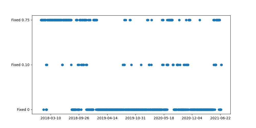
Figure 2: Estimated Policy. The estimated optimal policy derived from Algorithm 1 using rewards obtained from a quadratic utility (Section 2.1.3) is plotted for different values of the cost parameter ${\rm cost}=10^{-4}\times 2.5$ and $10^{-4}\times 7.5$ for panel (a) and (b), respectively.

(a)

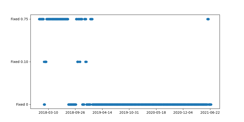
(b)

6 Conclusion

This paper considered the problem of optimally switching between models based on some observable state variables. Optimality is in terms of a discounted utility that is separable in time. The novelty is that the procedure is agnostic about the procedure used to construct the models and allows to account for costs when switching between models. The cost of switching model can be explicitly modelled, as in a portfolio problem, or modelled implicitly via a state dependent utility function, as long as this is separable in time. The possibility of switching between models accounting for costs changes the nature of the model selection problem. We now face a stochastic dynamic programming problem, as our choice at each point in time affects our future decisions. When the state space is large and/or continuous, this becomes a hard problem to solve. We bypass it by using a reinforcement learning algorithm that allows us to back up an estimated policy that is consistent for the true unobservable one, under relatively weak assumptions. The algorithm that we introduce is simple to use and computationally efficient. Numerical results via simulations show that the method has good finite sample properties. The simulations also show that when there is a cost in switching between models, using the model with the best one-step ahead forecasts is clearly suboptimal, as expected. We illustrate the power of the proposed methodology using a portfolio applications to trade the stocks on the S&P500 under rebalancing costs. The results show that the procedure is able to switch between portfolio models based on states of the world that depend on a number of macroeconomic variables such as interest rates spread, credit spreads and inflation.

Supplementary Material to “Action-State Dependent Dynamic Model Selection” by F. Cordoni and A. Sancetta

S.1 Proofs

The proofs of the main result use a standard coupling for beta mixing random variables. This allows us to adapt existing inequalities for independent identically distributed (i.i.d.) observations to the dependent case (Section S.1.1). The inequalities are based on the covering number of some function classes within which the various estimated quantities lie (Section S.1.2).

When stating results, we shall control the complexity of function classes using covering numbers. Recall the notation from Section 3.2. For a norm $\left|\cdot\right|_{p,\mathbb{Q}}$, the $\epsilon$-covering number of a class of functions $\mathcal{G}$ is the minimum number of balls of radius $\epsilon$, under $\left|\cdot\right|_{p,\mathbb{Q}}$, required to cover $\mathcal{G}$. We denote this covering number by $N\left(\epsilon,\mathcal{G},\left|\cdot\right|_{p,\mathbb{Q}}\right)$. An envelope function for $\mathcal{G}$ is a function $F$ such that $\left|f\right|\leq F$ for all $f\in\mathcal{G}$. The minimal envelope function is $F:=\sup_{f\in\mathcal{G}}\left|f\right|$. We shall assume that every quantity is measurable in what follows given that our sets are finite dimensional and often compact.

S.1.1 Inequalities for Dependent Random Variables

Throughout this section, the notation is intended to be local with no reference to the rest of the paper. This is to avoid the introduction of too many new symbols. We use $P_{n}$ to denote the empirical law of a stationary sample $\left\{X_{i}:i=1,2,..,n\right\}$ with values in a set $\mathcal{X}$. The following blocking technique is standard (Yu, 1994, Rio, 2017, Ch.8). Divide the sample into $2m$ nonoverlapping blocks of size $q$ each, plus a residual block of size $n-2mq$. To avoid distracting technicalities and notational trivialities in the remaining of the paper we suppose that $2mq=n$. The general case with a remainder is dealt with in the aforementioned references. Define $H_{i}=\left\{j\leq n:1+2\left(i-1\right)q\leq j\leq\left(2i-1\right)q\right\}$, $i\in\left\{1,2,...,m\right\}$. Let $\left(\tilde{X}_{j}\right)_{j\in H_{i}}$ be random variables with same law as $\left(X_{j}\right)_{j\in H_{i}}$ and s.t. $\left(\tilde{X}_{j}\right)_{j\in H_{i}}$ and $\left(\tilde{X}_{j}\right)_{j\in H_{k}}$ are independent for $i\neq k$. Define $P_{q,m}$ to be the measure that assigns weight $2/n$ to each variable in $\left\{\left(\tilde{X}_{j}\right):j\in\bigcup_{i=1}^{m}H_{i}\right\}$. Hence, the empirical measure $P_{q,m}$ is over variables within blocks of cardinality $q$, separated by $q$ variables and such that each block of variables is independent of each other. The following is a rephrasing of Lemma 4.1 Yu (1994).

Lemma S.1

Using the above notation, let

$$X_{H}:=\left\{\left(X_{j}\right):j\in\bigcup_{i=1}^{m}H_{i}\right\}\text{ and }\tilde{X}_{H}:=\left\{\left(\tilde{X}_{j}\right):j\in\bigcup_{i=1}^{m}H_{i}\right\}.$$

For any measurable function $G$ on $\mathcal{X}^{qm}$, uniformly bounded by one, $\mathbb{E}G\left(X_{H}\right)\leq\mathbb{E}G\left(\tilde{X}_{H}\right)+m\beta_{q}.$

Lemma S.2

Suppose that $\mathcal{F}$ is a class of functions with an envelope function $F$ satisfying the following: (1) $\left|F\right|_{2,P}<\infty$, (2) $\sup_{\mathbb{Q}}\ln N\left(\epsilon\left|F\right|_{2,\mathbb{Q}},\mathcal{F},\left|\cdot\right|_{2,\mathbb{Q}}\right)\leq A_{1}\ln\left(\frac{A_{2}}{\epsilon}\right)$ for some $A_{1},A_{2}>1$, where the supremum is over all discrete probability measures on $\mathcal{X}$ s.t. $\left|F\right|_{2,\mathbb{Q}}>0$. Then, for any $x>0$,

$$\Pr\left(\sup_{f\in\mathcal{F}}\left|\left(P_{q,m}-P\right)f\right|\geq x\right)\lesssim\frac{\left|F\right|_{2,P}\sqrt{1+A_{1}\ln A_{2}}}{x\sqrt{m}}.$$

Proof. Define $Z_{i,q}:=\left(\tilde{X}_{j}\right)_{j\in H_{i}}$ and let $P_{m|Z}$ to be the law that assigns weight $1/m$ to each variable in $\left\{Z_{i,q}:i=1,2,...,m\right\}$. Hence, the variables $Z_{i,q}$ are independent of each other. Let $P_{Z}$ be the law of $Z_{i,q}$. For any class of functions $\mathcal{F}$ on $\mathcal{X}$, let $\mathcal{F}\left(q\right):=\left\{g\left(z\right)=\frac{1}{q}\sum_{l=1}^{q}f\left(z_{l}\right):f\in\mathcal{F},z\in\mathcal{X}^{q}\right\}$; $\mathcal{X}^{q}=\otimes_{l=1}^{q}\mathcal{X}$ and if $z$ is a $q$-dimensional tuple of elements in $\mathcal{X}$, $z_{l}$ is the $l^{th}$ entry. Then, the set $\left\{\sup_{f\in\mathcal{F}}\left|\left(P_{q,m}-P\right)f\right|\geq x\right\}$ is contained in the set $\left\{\sup_{f\in\mathcal{F}\left(q\right)}\left|P_{m|Z}-P_{Z}f\right|\geq x\right\}$. From the first display on page 240 of van der Vaart and Wellner (2000) we deduce that

$$\left|\sqrt{m}\sup_{f\in\mathcal{F}\left(q\right)}\left|\left(P_{m|Z}-P_{Z}\right)f\right|\right|_{2,P_{Z}}\lesssim\mathbb{E}\int_{0}^{\eta\left(q\right)}\sqrt{1+\ln N\left(\epsilon,\mathcal{F}\left(q\right),\left|\cdot\right|_{2,P_{m|Z}}\right)}d\epsilon,$$

where $\eta\left(q\right):=\left|\sup_{f\in\mathcal{F}\left(q\right)}\left|f\right|\right|_{2,P_{m|Z}}$. By Jensen inequality, $\eta\left(q\right)\leq\eta:=\left|\sup_{f\in\mathcal{F}}\left|f\right|\right|_{2,P_{q,m}}$. Moreover, for $h_{1},h_{2}\in\mathcal{F}\left(q\right)$, such that $h_{k}\left(z\right)=\frac{1}{q}\sum_{l=1}^{q}f_{k}\left(z_{l}\right)$, $f_{k}\in\mathcal{F}$, $k=1,2$, using again Jensen inequality, $\left|h_{1}-h_{2}\right|_{2,P_{m|Z}}^{2}\leq\left|f_{1}-f_{2}\right|_{2,P_{q,m}}^{2}$, using the definition of $P_{q,m}$. We can then deduce that the r.h.s. of the above display is less than

$$\mathbb{E}\int_{0}^{\eta}\sqrt{1+\ln N\left(\epsilon,\mathcal{F},\left|\cdot\right|_{2,P_{q,m}}\right)}d\epsilon\leq\mathbb{E}\left[\left|F\right|_{2,P_{q,m}}\int_{0}^{1}\sqrt{1+\ln N\left(\epsilon\left|F\right|_{2,P_{q,m}},\mathcal{F},\left|\cdot\right|_{2,P_{q,m}}\right)}d\epsilon\right]$$

where the second inequality follows by change of variables and using a trivial upper bound in the upper limit of the integral. Taking the supremum over all discrete probability measures on $\mathcal{X}$ such that $\mathbb{Q}F^{2}>0$, and using Jensen inequality, we deduce that the r.h.s. of the above display is less than

$$\left|F\right|_{2,P}\sup_{\mathbb{Q}}\int_{0}^{1}\sqrt{1+\ln N\left(\epsilon\left|F\right|_{2,\mathbb{Q}},\mathcal{F},\left|\cdot\right|_{2,\mathbb{Q}}\right)}d\epsilon.$$

We can then substitute the bound on the logarithm of the covering number and compute the integral to deduce the statement of the lemma by an application of Markov inequality to bound the probability.  

The following is a rephrasing of Lemma 16 in Lazaric et al. (2012) using the bound implied by a uniform entropy condition. It is the analogue of Theorem 11.2 in in Gÿorfi (2002), but for dependent data.

Lemma S.3

Suppose that $\left(X_{t}\right)_{t\geq 1}$ is a sequence of stationary random variables with values in $\mathcal{X}$ and beta mixing coefficients $\beta_{q}$, $q\geq 0$. Suppose that $\mathcal{F}$ is a class of functions with an envelope function $F$ satisfying the following: (1) $F\leq M$ for some finite constant $M$, and (2) $\sup_{\mathbb{Q}}\ln N\left(\epsilon M,\mathcal{F},\left|\cdot\right|_{2,\mathbb{Q}}\right)\leq A_{1}\ln\left(\frac{A_{2}}{\epsilon}\right)$, where the supremum is over all discrete probability measures on $\mathcal{X}$ such that $\left|F\right|_{2,\mathbb{Q}}>0$. Define integers $q$ and $m$ as in Lemma S.1. Then, for any $x>0$ such that $mx\rightarrow\infty$,

$$\Pr\left(\sup_{f\in\mathcal{F}}\left(\left|f\right|_{2,P}-2\left|f\right|_{2,P_{n}}\right)>x\right)\lesssim\left(\frac{24A_{2}M}{\sqrt{2}x}\right)^{A_{1}}\exp\left\{-\frac{mx^{2}}{288M^{2}}\right\}+m\beta_{q}.$$

The same bound holds for $\Pr\left(\sup_{f\in\mathcal{F}}\left(\left|f\right|_{2,P_{n}}-2^{3/2}\left|f\right|_{2,P}\right)>x\right)$.

S.1.2 Bounds on Uniform Covering Numbers of Function Classes

We need to introduce some additional notation. In particular, for later reference, we introduce a relatively long list of function classes that will be used in the proof.

S.1.2.1 Function Classes

We introduce the following function classes, some of which have already been defined previously:

$\mathcal{F}_{B}$:= Real valued functions $h$ on $\mathcal{S}$ s.t. $h=\left[\sum_{k=1}^{K}b_{k}\varphi_{k}\left(s\right)\right]_{B}$ (see (8));

$\mathcal{F}_{B}^{\mathcal{A}}$:= Real valued functions $h$ on $\mathcal{S}\times\mathcal{A}$ s.t. $\mathcal{S}\times\mathcal{A}\ni\left(s,a\right)\mapsto h\left(s,a\right)=\sum_{a^{\prime}\in\mathcal{A}}f_{a^{\prime}}\left(s\right)1_{\left\{a^{\prime}=a\right\}}$ where each $f_{a^{\prime}}$ is in $\mathcal{F}_{B}$;

$\mathcal{F}_{B}^{\max}$:= Real valued functions $h$ on $\mathcal{S}$ s.t. $h\left(s\right)=\max_{a\in\mathcal{A}}f\left(s,a\right)$ where $f\in\mathcal{F}_{B}^{\mathcal{A}}$;

$\mathbb{K}^{a}\mathcal{\mathcal{F}^{\max}}$:= Real valued functions $h$ on $\mathcal{S}$ s.t. $h\left(s,a\right)=\left(\mathbb{K}^{a}f\right)\left(s\right)$ where $f\in\mathcal{F}_{B}^{\max}$;

$\mathbb{K}^{\max}\mathcal{\mathcal{F}^{\max}}$:= Real valued functions $h$ on $\mathcal{S}$ s.t. $h\left(s\right)=\max_{a\in\mathcal{A}}\left(\mathbb{K}^{a}f\right)\left(s\right)$ where $f\in\mathcal{F}_{B}^{\max}$;

If $f\in\mathcal{F}_{B}^{\mathcal{A}}$, then $f\left(\cdot,a\right)=\sum_{a^{\prime}\in\mathcal{A}}f_{a^{\prime}}\left(\cdot\right)1_{\left\{a^{\prime}=a\right\}}=f_{a}$ where $f_{a}\in\mathcal{F}_{B}$ and this implies that $\sum_{a\in\mathcal{A}}f\left(\cdot,a\right)=\sum_{a\in\mathcal{A}}f_{a}$. Hence, each element in $\mathcal{F}_{B}^{\mathcal{A}}$ is a collection of $\left|\mathcal{A}\right|$ elements in $\mathcal{F}_{B}$ where the second argument in $f\in\mathcal{F}_{B}^{\mathcal{A}}$ says which element is to be picked. Given that $\mathcal{F}_{B}^{\mathcal{A}}$ is a space of capped linear functions, we have that $f-g\in\mathcal{F}_{2B}^{\mathcal{A}}$ for any $f,g\in\mathcal{F}_{B}^{\mathcal{A}}$. Recalling the definition of the cap operator $\left[\cdot\right]_{B}$ in Section 3.3, and hence the fact that it is not linear. We also have that $\Pi_{n,B}f\in\mathbf{\mathcal{F}}_{B}$ for any real valued function on $\mathcal{S}$. Note that $\Pi_{n,B}$ is not a linear operator.

S.1.2.2 Lemmas on Covering Numbers of the Function Classes

The aim of this section is to compute the covering number of the classes of functions defined in Section S.1.2.1. At first, we break down the calculation in terms of simpler function classes. In what follows, for any classes of functions $\mathcal{F}$ and $\mathcal{G}$, $\mathcal{F}\oplus\mathcal{G}:=\left\{h=f+g:f\in\mathcal{F},g\in\mathcal{G}\right\}$ and $\mathcal{F}\otimes\mathcal{G}:=\left\{h=fg:f\in\mathcal{F},g\in\mathcal{G}\right\}$.

Lemma S.4

Suppose that $\mathbb{Q}$ is a probability measure on a set $\mathcal{X}$ and $\mathcal{F}$ and $\mathcal{G}$ are classes of functions on $\mathcal{X}$ with an envelope function $F$ and $G$, respectively. Then, for any strictly positive constants $c_{1}$, $c_{2}$ s.t. $c_{1}+c_{2}=1$, we have that $N\left(\epsilon,\mathcal{F}\oplus\mathcal{G},\left|\cdot\right|_{p,\mathbb{Q}}\right)\leq N\left(c_{1}\epsilon,\mathcal{F},\left|\cdot\right|_{p,\mathbb{Q}}\right)N\left(c_{2}\epsilon,\mathcal{G},\left|\cdot\right|_{p,\mathbb{Q}}\right)$. If the envelope functions are uniformly bounded, we have that $N\left(\epsilon,\mathcal{F}\otimes\mathcal{G},\left|\cdot\right|_{p,\mathbb{Q}}\right)\leq N\left(\epsilon c_{1}\left|G\right|_{\infty}^{-1},\mathcal{F},\left|\cdot\right|_{p,\mathbb{Q}}\right)N\left(\epsilon c_{2}\left|F\right|_{\infty}^{-1},\mathcal{G},\left|\cdot\right|_{p,\mathbb{Q}}\right)$

Proof. For the $L_{1}$ empirical norm $\left|\cdot\right|_{1,P_{n}}$, the statements are Theorems 29.6 and 29.7 in Devroye et al. (1997). Inspection of the proofs show that the extension to $\left|\cdot\right|_{p,\mathbb{Q}}$ is immediate by application of the triangle inequality.  

Lemma S.5

Let $F$ be an envelope function for $\mathcal{F}_{B}$. Then, $\sup_{\mathbb{Q}}\ln N\left(\epsilon\left|F\right|_{2,\mathbb{Q}},\mathcal{F}_{B},\left|\cdot\right|_{2,\mathbb{Q}}\right)\lesssim K\ln\left(\frac{1}{\epsilon}\right)$, $\epsilon>0$, where the supremum is over all discrete probability measures on $\mathcal{S}$ s.t. $\left|F\right|_{2,\mathbb{Q}}>0$.

Proof. The functions in $\mathcal{F}_{B}$ are nondecreasing transformation of the functions in $\mathcal{F}$. Hence, they have the same VC index/pseudo dimension (Theorem 11.3 in Anthony and Bartlett, 1999; see also Lemma 2.6.18(viii) in van der Vaart and Wellner, 2000). Given that $\mathcal{F}$ is a $K$-dimensional vector, its pseudo dimension is $K$ (Theorem 11.4 in Anthony and Bartlett, 1999; see also Lemma 2.6.15 in van der Vaart and Wellner, 2000). Then, we apply Theorem 2.6.7 in van der Vaart and Wellner (2000) to bound the uniform covering number by the pseudo dimension, as given in the statement of the lemma.  

The above result allows us to control the following function classes.

Lemma S.6

Let $F$ be an envelope function for $\mathcal{F}_{B}$. Under the assumptions of Lemma S.5 we have the following:
1. $\sup_{\mathbb{Q}}\ln N\left(\epsilon\left|F\right|_{\mathbb{Q}},\mathcal{F}_{B}^{\max},\left|\cdot\right|_{p,\mathbb{Q}}\right)\lesssim\left|\mathcal{A}\right|K\ln\left(\frac{1}{\epsilon}\right)$, where $F$ is an envelope function for $\mathcal{F}_{B}$;
2. $\sup_{\mathbb{Q}}\ln N\left(\epsilon\left|F\right|_{\mathbb{Q}},\mathbb{K}^{a}\mathcal{F}_{B}^{\max},\left|\cdot\right|_{p,\mathbb{Q}}\right)\lesssim\left|\mathcal{A}\right|K\ln\left(\frac{\left|\mathcal{A}\right|}{\epsilon}\right)$;
3. $\sup_{\mathbb{Q}}\ln N\left(\epsilon\left|F\right|_{\mathbb{Q}},\mathbb{K}^{\max}\mathcal{F}_{B}^{\max},\left|\cdot\right|_{p,\mathbb{Q}}\right)\lesssim\left|\mathcal{A}\right|K\ln\left(\frac{\left|\mathcal{A}\right|}{\epsilon}\right)$;
4. $\ln N\left(\epsilon\left|F\right|_{\mathbb{Q}},h\mathcal{F}_{B},\left|\cdot\right|_{p,\mathbb{Q}}\right)\lesssim K\ln\left(\frac{M}{\epsilon}\right)$, where $h\mathcal{F}_{B}$ is the set of functions $hf$ where $f\in\mathcal{F}_{B}$ and $h$ is a fixed function whose absolute value is bounded by $M$;
5. $N\left(\epsilon,\mathbb{K}^{\max}f,\left|\cdot\right|_{p,\mathbb{Q}}\right)\lesssim\ln\left|\mathcal{A}\right|$ for any fixed function $f$ uniformly bounded on $\mathcal{S}$.

Proof. We prove each point separately.

Point 1.

For any $f,g\in\mathcal{F}_{B}^{\mathcal{A}}$,

$$\left|\max_{a\in\mathcal{A}}f\left(\cdot,a\right)-\max_{a\in\mathcal{A}}g\left(\cdot,a\right)\right|_{p,\mathbb{Q}}\leq\left|\max_{a\in\mathcal{A}}\left|f\left(\cdot,a\right)-g\left(\cdot,a\right)\right|\right|_{p,\mathbb{Q}}.$$

Then, note that for $f,g\in\mathcal{F}_{B}^{\mathcal{A}}$, $\max_{a\in\mathcal{A}}\left|f\left(\cdot,a\right)-g\left(\cdot,a\right)\right|=\max_{a\in\mathcal{A}}\left|f_{a}\left(\cdot\right)-g_{a}\left(\cdot\right)\right|$ where $f_{a},g_{a}\in\mathcal{F}_{B}$. This follows from the definition of $\mathcal{F}_{B}^{\mathcal{A}}$. Then, by definition of functions in $\mathcal{F}_{B}^{\max}$, the $\epsilon$-covering number of $\mathcal{F}_{B}^{\max}$ is bounded by $\left[N\left(\epsilon,\mathcal{F}_{B},\left|\cdot\right|_{p,\mathbb{Q}}\right)\right]^{\left|\mathcal{A}\right|}$, as there are $\left|\mathcal{A}\right|$ functions in $\mathcal{F}_{B}$ to control at the same time. Using Lemma S.5 and taking the logarithm gives the result.

Point 2.

For $f$ and $g$ as in the proof of the previous point,

$$\left|\left(\mathbb{K}^{a}\max_{a^{\prime}\in\mathcal{A}}f\left(\cdot,a^{\prime}\right)\right)-\left(\mathbb{K}^{a}\max_{a^{\prime}\in\mathcal{A}}g\left(\cdot,a^{\prime}\right)\right)\right|_{p,\mathbb{Q}}\leq\left|\sum_{a^{\prime}\in\mathcal{A}}\left|\mathbb{K}^{a}f\left(\cdot,a^{\prime}\right)-\mathbb{K}^{a}g\left(\cdot,a^{\prime}\right)\right|\right|_{p,\mathbb{Q}}.$$

Using Jensen inequality because $\left|\mathcal{A}\right|$ is finite, we deduce that the r.h.s. is less than

$$\left[\left|\mathcal{A}\right|^{p-1}\sum_{a^{\prime}\in\mathcal{A}}\left|\mathbb{K}^{a}f\left(\cdot,a^{\prime}\right)-\mathbb{K}^{a}g\left(\cdot,a^{\prime}\right)\right|_{p,\mathbb{Q}}^{p}\right]^{1/p}\leq\left|\mathcal{A}\right|^{\frac{p-1}{p}}\sum_{a^{\prime}\in\mathcal{A}}\left|\left(\mathbb{K}^{a}f\left(\cdot,a^{\prime}\right)-\mathbb{K}^{a}g\left(\cdot,a^{\prime}\right)\right)\right|_{p,\mathbb{Q}}$$

where the r.h.s. follows by concavity of of the function $x^{1/p}$ for $x\geq 0$. Denote by $\mathbb{Q}\mathbb{K}^{a}$ the probability measure such that $\mathbb{Q}\mathbb{K}^{a}f=\int_{\mathcal{S}}\int_{\mathcal{S}}f\left(s\right)\kappa^{a}\left(r,ds\right)d\mathbb{Q}\left(r\right)$. Then, by Jensen inequality the above display is less than

$$\left|\mathcal{A}\right|^{\frac{p-1}{p}}\sum_{a^{\prime}\in\mathcal{A}}\left|f\left(\cdot,a^{\prime}\right)-g\left(\cdot,a^{\prime}\right)\right|_{p,\mathbb{Q}\mathbb{K}^{a}}.$$

By the same argument as in the proof of Point 1 above, we deduce the the above is less than

$$\left|\mathcal{A}\right|^{\frac{p-1}{p}}\sum_{a^{\prime}\in\mathcal{A}}\left|f_{a^{\prime}}\left(\cdot\right)-g_{a^{\prime}}\left(\cdot\right)\right|_{p,\mathbb{Q}\mathbb{K}^{a}}$$

where $f_{a^{\prime}},g_{a^{\prime}}\in\mathcal{F}_{B}$. Then, by definition of the functions in $\mathbb{K}^{a}\mathcal{F}_{B}^{\max}$, the $\epsilon$-covering number of $\mathbb{K}^{a}\mathcal{F}_{B}^{\max}$ under $\left|\cdot\right|_{p,\mathbb{Q}}$ is bounded by $\left[N\left(\left|\mathcal{A}\right|^{-\frac{2p-1}{p}}\epsilon,\mathcal{F}_{B},\left|\cdot\right|_{p,\mathbb{Q}\mathbb{K}^{a}}\right)\right]^{\left|\mathcal{A}\right|}$. We use Lemma S.5 and the fact that it holds for any probability measure to infer the result after taking the logarithm.

Proof of Point 3.

By the same arguments as in the proof of the previous points,

$$\left|\max_{a\in\mathcal{A}}\mathbb{K}^{a}\max_{a^{\prime}\in\mathcal{A}}f\left(\cdot,a^{\prime}\right)-\max_{a\in\mathcal{A}}\mathbb{K}^{a}\max_{a^{\prime}\in\mathcal{A}}g\left(\cdot,a^{\prime}\right)\right|_{p,\mathbb{Q}}$$

$$\leq \left|\mathcal{A}\right|^{1/p}\max_{a\in\mathcal{A}}\left|\mathbb{K}^{a}\max_{a^{\prime}\in\mathcal{A}}f\left(\cdot,a^{\prime}\right)-\mathbb{K}^{a}\max_{a^{\prime}\in\mathcal{A}}g\left(\cdot,a^{\prime}\right)\right|_{p,\mathbb{Q}}.$$

Then, by definition of the functions in $\mathbb{K}^{\max}\mathcal{F}_{B}^{\max}$, the $\epsilon$-covering number of $\mathbb{K}^{\max}\mathcal{F}_{B}^{\max}$ is bounded by $\prod_{a\in\mathcal{A}}N\left(\epsilon\left|\mathcal{A}\right|^{-1/p},\mathbb{K}^{a}\mathcal{F}_{B}^{\max},\left|\cdot\right|_{p,\mathbb{Q}}\right)$. Discarding unnecessary constants, the result follows from Point 2.

Proof of Point 4.

This is a special case of Lemma S.4 because $h$ is fixed and bounded.

Proof of Point 5.

Given that $f$ is fixed, this follows from Lemma 2.2.2 in van der Vaart and Wellner (2000).  

S.1.3 Convergence Rates for the Capped Projection Operator

At first, we introduce some properties of the capped projection operator. The next is a property also shared by standard projections and useful to bound their estimation error.

Lemma S.7

For any $f:\mathcal{X}\rightarrow\mathbb{R}$ and $B\geq 0$, we have that $\left|\Pi_{n,B}f\right|_{2,P_{n}}^{2}\leq 2P_{n}f\Pi_{n,B}f$.

Proof. It is clear that $0$ is a solution to the minimization problems implied by (7) and (9). Therefore,

$$\left|f-\Pi_{n}f\right|_{2,P_{n}}+{\rm Pen}\left(\Pi_{n}f\right)+\left|\Pi_{n}f-\Pi_{n,B}f\right|_{2,P_{n}}\leq\left|f\right|_{2,P_{n}}.$$

By the triangle inequality and the above, we deduce that $\left|f-\Pi_{n,B}f\right|_{2,P_{n}}\leq\left|f\right|_{2,P_{n}}$. Taking squares of this last inequality and rearranging we obtain the statement of the lemma.  

The capped projection operator is superadditive.

Lemma S.8

For any $f,g:\mathcal{S}\rightarrow\mathbb{R}$ and $B\geq 0$, we have that $\left|\Pi_{n,B}f\left(s\right)-\Pi_{n,B}g\left(s\right)\right|\leq\left|\Pi_{n,2B}\left(f-g\right)\left(s\right)\right|$ uniformly in $s\in\mathcal{S}$.

Proof. By definition of the operator $\Pi_{n,B}$ and linearity of $\Pi_{n}$, we have that $\Pi_{n,2B}\left(f-g\right)=\left[\Pi_{n}f-\Pi_{n}g\right]_{2B}$. To deduce the result, note that $\left|\left[x\right]_{B}-\left[y\right]_{B}\right|\leq\left|\left[x-y\right]_{2B}\right|$ for any $x,y\in\mathbb{R}$.  

Next we derive the convergence rates of the capped projection operator for some function classes that satisfy a martingale and uniform entropy condition. To this end, recall the definition of the cap operator $\left[\cdot\right]_{M}$ with cap $M$ rather than $B$ in Section 3.3.

Lemma S.9

Let $\mathcal{H}$ be a class of functions on $\mathcal{S}$ s.t. $\max_{a\in\mathcal{A}}\left|\mathbb{K}^{a}h\right|=0$, $h\in\mathcal{H}$, with an envelope function $F_{\mathcal{H}}$ s.t. $\left|F_{\mathcal{H}}\right|_{v,P}<\infty$, $v\geq 2$. Let $\mathcal{H}_{M}$ be the class of functions $\left[h\right]_{M}$ where $h\in\mathcal{H}$, with envelope function $F_{\mathcal{H}_{M}}$. Suppose that for any $M\geq\left(B\left|F_{\mathcal{H}}\right|_{v,P}^{v}\right)^{\frac{1}{v-1}}$, $\sup_{\mathbb{Q}}\ln N\left(\epsilon\left|F_{\mathcal{H}_{M}}\right|_{2,\mathbb{Q}},\mathcal{H}_{M},\left|\cdot\right|_{2,\mathbb{Q}}\right)\leq A_{1}\ln\left(\frac{A_{2}}{\epsilon}\right)$, for some $A_{1},A_{2}>1$, possibly diverging to infinity, where the supremum is over all discrete distributions on $\mathcal{S}$ s.t. $\left|F_{\mathcal{H}_{M}}\right|_{2,\mathbb{Q}}>0$. Define $\mathcal{H}\circ T$ to be the class of functions $h\left(T\cdot\right)$, $h\in\mathcal{H}$. Under the Assumptions, $\sup_{h\in\mathcal{\mathcal{H}}\circ T}\left|\Pi_{n,B}h\right|_{2,P_{n}}=O_{P}\left(r_{n}^{-1}\right)$ where

$$r_{n}:=\left(\frac{n}{\left(A_{1}\ln\left(BA_{2}\right)+K\right)\ln n}\right)^{\frac{v-1}{2\left(v+1\right)}}\left(B\left|F_{\mathcal{H}}\right|_{v,P}^{v}\right)^{-\frac{1}{\left(v+1\right)}}.$$

Proof. Fix a large integer $l_{0}$ and define the event

$$\mathcal{E}_{0}:=\left\{\exists h\in\mathcal{H}\circ T:\left|\Pi_{n,B}h\right|_{2,P}>2^{l_{0}}r_{n}^{-1}\right\}.$$

From Lemma S.7, adding and subtracting $\left|\Pi_{n,B}h\right|_{2,P}^{2}$, deduce that the event

$$\mathcal{E}_{1}:=\left\{\exists h\in\mathcal{H}\circ T:2P_{n}h\Pi_{n,B}h+\left|\Pi_{n,B}h\right|_{2,P}^{2}-\left|\Pi_{n,B}h\right|_{2,P_{n}}^{2}\geq\left|\Pi_{n,B}h\right|_{2,P}^{2}\right\}$$

is always true. Hence, deduce that $\mathcal{E}_{0}\subseteq\mathcal{E}_{1}\cap\mathcal{E}_{0}$ . Define

$$\mathcal{E}_{1,1}:=\left\{\exists h\in\mathcal{H}\circ T,f\in\mathcal{F}_{B}:2P_{n}hf\geq\frac{1}{2}\left|\Pi_{n,B}h\right|_{2,P}^{2}\text{ and }\left|f\right|_{2,P}^{2}>\frac{2^{2l_{0}}}{r_{n}^{2}}\right\}$$

$$\mathcal{E}_{1,2}:=\left\{\exists h\in\mathcal{H}\circ T,f\in\mathcal{F}_{B}:\left|f\right|_{2,P}^{2}-\left|f\right|_{2,P_{n}}^{2}\geq\frac{1}{2}\left|f\right|_{2,P}^{2}\text{ and }\left|f\right|_{2,P}^{2}>\frac{2^{2l_{0}}}{r_{n}^{2}}\right\}.$$

Using the elementary set inequality $\left\{x,y\in\mathbb{R}:x+y\geq c\right\}\subseteq\left\{x\in\mathbb{R}:x\geq c/2\right\}\cup\left\{y\in\mathbb{R}:y\geq c/2\right\}$ for any constant $c$, we deduce that $\mathcal{E}_{0}\subseteq\mathcal{E}_{1,1}\cup\mathcal{E}_{1,2}$. Let $P_{n|H}$ be the empirical measure that assigns mass $2/n$ to the points in $\left\{S_{i}:i\in\bigcup_{j=1}^{m}H_{j}\right\}$. To avoid inconsequential complications, we suppose that $2qm=n$. By the elementary set inequality, the last remark and stationarity, we find that $\Pr\left(\mathcal{E}_{1,k}\right)\leq 2\Pr\left(\mathcal{E}_{1,k}^{\prime}\right)$, $k=1,2$, where

$$\mathcal{E}_{1,1}^{\prime}:=\left\{\exists h\in\mathcal{H}\circ T,f\in\mathcal{F}_{B}:2P_{n|H}hf\geq\frac{1}{2}\left|f\right|_{2,P}^{2}\text{ and }\left|f\right|_{2,P}^{2}>\frac{2^{2l_{0}}}{r_{n}^{2}}\right\}.$$

$$\mathcal{E}_{1,2}^{\prime}:=\left\{\exists f\in\mathcal{F}_{B}:\left|f\right|_{2,P}^{2}-\left|f\right|_{2,P_{n|H}}^{2}\geq\frac{1}{2}\left|f\right|_{2,P}^{2}\text{ and }\left|f\right|_{2,P}^{2}>\frac{2^{2l_{0}}}{r_{n}^{2}}\right\}.$$

By Lemma S.1 applied to the indicator function $1_{\mathcal{E}_{1,k}^{\prime}}$, we deduce that

$$\Pr\left(\mathcal{E}_{0}\right)\leq 2\Pr\left(\mathcal{E}_{2,1}\right)+2\Pr\left(\mathcal{E}_{2,2}\right)+4m\beta_{q},$$

where

$$\mathcal{E}_{2,1}:=\left\{\exists h\in\mathcal{H}\circ T,f\in\mathcal{F}_{B}:2P_{q,m}hf\geq\frac{1}{2}\left|f\right|_{2,P}^{2}\text{ and }\left|f\right|_{2,P}^{2}>\frac{2^{2l_{0}}}{r_{n}^{2}}\right\}$$

and

$$\mathcal{E}_{2,2}:=\left\{\exists f\in\mathcal{F}_{B}:\left|f\right|_{2,P}^{2}-\left|f\right|_{2,P_{q,m}}^{2}\geq\frac{1}{2}\left|f\right|_{2,P}^{2}\text{ and }\left|f\right|_{2,P}^{2}>\frac{2^{2l_{0}}}{r_{n}^{2}}\right\}.$$

By Assumption 2, we choose $q=\left(1/C_{\beta}\right)\ln n$ ($C_{\beta}$ as in Assumption 2) so that $m\beta_{q}\rightarrow 0$. This implies that $m\asymp n/\ln n$ and we shall replace $m$ with the r.h.s., in due course.

We shall only focus on showing that $\Pr\left(\mathcal{E}_{2,1}\right)$ can be arbitrarily small for large enough $l_{0}$, as defined at the start of the proof. The same arguments, though simpler, can be applied to $\Pr\left(\mathcal{E}_{2,2}\right)$ as well. Define the two events

$$\mathcal{E}_{3}:=\left\{\exists h\in\mathcal{H}\circ T,f\in\mathcal{F}_{B}:2P_{q,m}\left[h\right]_{M}f\geq\frac{1}{4}\left|f\right|_{2,P}^{2}\text{ and }\left|f\right|_{2,P}^{2}>\frac{2^{2l_{0}}}{r_{n}^{2}}\right\}$$

$$\mathcal{E}_{4}:=\left\{\exists h\in\mathcal{H}\circ T,f\in\mathcal{F}_{B}:2P_{q,m}\left(h-\left[h\right]_{M}\right)f\geq\frac{2^{2l_{0}}}{4r_{n}^{2}}\right\}.$$

Then, by the usual basic set inequality, $\mathcal{E}_{2,1}\subseteq\mathcal{E}_{3}\cup\mathcal{E}_{4}$. By this remark and the union bound, we deduce that $\Pr\left(\mathcal{E}_{2,1}\right)\leq\Pr\left(\mathcal{E}_{3}\right)+\Pr\left(\mathcal{E}_{4}\right)$. The last term on the r.h.s. can be made small by suitable choice of $M$. In fact, nothing that $\sup_{h\in\mathcal{H}}\left|\left(h-\left[h\right]_{M}\right)\right|\leq F_{\mathcal{H}}1_{\left\{F_{\mathcal{H}}>M\right\}}$, by Markov inequality,

$$\Pr\left(\mathcal{E}_{4}\right)\leq\frac{4r_{n}^{2}}{2^{2j_{0}}}BPF_{\mathcal{H}}1_{\left\{F_{\mathcal{H}}>M\right\}}\leq\frac{4r_{n}^{2}}{2^{2j_{0}}}B\left|F_{\mathcal{H}}\right|_{v,P}\left(\left|F_{\mathcal{H}}\right|_{v,P}/M\right)^{\left(v-1\right)}$$

using Holder inequality in the second inequality together with Markov inequality once again but for a $v$ moment. Hence, we set

$$M=\left(r_{n}^{2}B\left|F_{\mathcal{H}}\right|_{v,P}^{v}\right)^{\frac{1}{v-1}}.$$ (S.1)

For $j_{0}$ large enough, the above display can be made arbitrarily small.

We now follow the proof of Theorem 3.2.5 in van der Vaart and Wellner (2000), but give some details because of nontrivial differences. First, note that

$$\left\{f\in\mathcal{F}_{B}:\left|f\right|_{2,P}>2^{l_{0}}r_{n}^{-1}\right\}\subseteq\bigcup_{l\geq l_{0}}\mathcal{F}_{B,l}$$

where

$$\mathcal{F}_{B,l}:=\left\{f\in\mathcal{F}_{B}:\left|f\right|_{2,P}\in\left(2^{l-1}r_{n}^{-1},2^{l}r_{n}^{-1}\right]\right\}.$$

Therefore, $\mathcal{E}_{3}\subseteq\bigcup_{l\geq l_{0}}\mathcal{E}_{3,l}$ where

$$\mathcal{E}_{3,l}:=\left\{\exists g\in\mathcal{H}_{M}\circ T,f\in\mathcal{F}_{B,l}:2P_{q,m}gf\geq\frac{1}{2}2^{2\left(l-1\right)}r_{n}^{-2}\right\}.$$

Then, by the union bound we deduce that $\Pr\left(\mathcal{E}_{3}\right)\leq\sum_{l\geq l_{0}}\Pr\left(\mathcal{E}_{3,l}\right)$. We shall now focus on a bound for the summation on the r.h.s.. An envelope function $F_{l}$ for $\mathcal{H}_{M}\otimes\mathcal{F}_{B,l}$ is given by $F_{l}=MF_{B,l}$ where $F_{B,l}:=\sup_{f\in\mathcal{F}_{B}}\left|f\right|1_{\left\{\left|f\right|_{2,P}\in\left(2^{l-1}r_{n}^{-1},2^{l}r_{n}^{-1}\right]\right\}}$. This implies that $\left|F_{l}\right|_{2,P}\leq M2^{l}r_{n}^{-1}$ but also that $\left|F_{l}\right|_{2,P}>M2^{l-1}r_{n}^{-1}$.We wish to apply Lemma S.2 to $\Pr\left(\mathcal{E}_{3,l}\right)$. To do so, with $\mathbb{Q}$ as in Lemma S.2, we compute an upper bound for

$$N\left(\epsilon\left|F_{l}\right|_{2,\mathbb{Q}},\mathcal{H}_{M}\otimes\mathcal{F}_{B,l},\left|\cdot\right|_{2,\mathbb{Q}}\right).$$ (S.2)

First note that the above is the same as

$$N\left(\epsilon,\tilde{\mathcal{H}}_{M}\otimes\tilde{\mathcal{F}}_{B,l},\left|\cdot\right|_{2,\mathbb{Q}}\right)$$

where $h\in\tilde{\mathcal{H}}_{M}$ if and only if $Mh\in\mathcal{H}_{M}$, and $\tilde{\mathcal{F}}_{B,l}$ is the class of functions $\mathcal{F}_{B,l}$ with diameter equal to one under the $\left|\cdot\right|_{2,\mathbb{Q}}$ norm. To see this, note that for $h_{i}\in\mathcal{H}_{M}$ and $f_{i}\in\mathcal{F}_{B,l}$, $i=1,2$,

$$\frac{\left|h_{1}f_{1}-h_{2}f_{2}\right|_{2,\mathbb{Q}}}{\left|F_{l}\right|_{2,\mathbb{Q}}}=\left|\frac{h_{1}}{M}\frac{f_{1}}{\left|F_{B,l}\right|_{2,\mathbb{Q}}}-\frac{h_{2}}{M}\frac{f_{2}}{\left|F_{B,l}\right|_{2,\mathbb{Q}}}\right|_{2,\mathbb{Q}}$$

so that $h_{i}/M\in\tilde{\mathcal{H}}_{M}$ and $\frac{f_{i}}{\left|F_{B,l}\right|_{2,\mathbb{Q}}}\in\tilde{\mathcal{F}}_{B,l}$. Hence, functions in $\tilde{\mathcal{H}}_{M}$ are uniformly bounded by one. Moreover, a ball of size $\epsilon\left|F_{l}\right|_{2,\mathbb{Q}}$ for $\mathcal{H}_{M}\otimes\mathcal{F}_{B,l}$ under $\left|\cdot\right|_{2,\mathbb{Q}}$, is a ball of size $\epsilon$ for $\tilde{\mathcal{H}}_{M}\otimes\tilde{\mathcal{F}}_{B,l}$ under the same norm. So, by Lemma S.4, we deduce that (S.2) is less than

$$N\left(\frac{\epsilon}{B},\tilde{\mathcal{H}}_{M},\left|\cdot\right|_{2,\mathbb{Q}}\right)N\left(\epsilon,\tilde{\mathcal{F}}_{B,l},\left|\cdot\right|_{2,\mathbb{Q}}\right).$$ (S.3)

However, $N\left(\frac{\epsilon}{B},\tilde{\mathcal{H}}_{M},\left|\cdot\right|_{2,\mathbb{Q}}\right)=N\left(\epsilon\frac{M}{B},\mathcal{H}_{M},\left|\cdot\right|_{2,\mathbb{Q}}\right)$ is smaller than $N\left(\epsilon B^{-1}\left|F_{\mathcal{H}_{M}}\right|_{2,\mathbb{Q}},\mathcal{H}_{M},\left|\cdot\right|_{2,\mathbb{Q}}\right)$ because $\left|F_{\mathcal{H}_{M}}\right|_{2,\mathbb{Q}}\leq M$. Moreover, $N\left(\epsilon,\tilde{\mathcal{F}}_{B,l},\left|\cdot\right|_{2,\mathbb{Q}}\right)=N\left(\epsilon\left|F_{B,l}\right|_{2,\mathbb{Q}},\mathcal{F}_{B,l},\left|\cdot\right|_{2,\mathbb{Q}}\right)$ is smaller than $N\left(\epsilon\left|F_{B}\right|_{2,\mathbb{Q}},\mathcal{F}_{B},\left|\cdot\right|_{2,\mathbb{Q}}\right)$ because $\mathcal{F}_{B,l}\subseteq\mathcal{F}_{B}$, where $F_{B}:=\sup_{f\in\mathcal{F}_{B}}\left|f\right|$ and $\mathcal{F}_{B}$ as in (8). By these remarks, the assumption of the lemma, and Lemma S.5, the logarithm of (S.3) is bounded by a constant multiple of

$$A_{1}\ln\left(\frac{BA_{2}}{\epsilon}\right)+K\ln\left(\frac{1}{\epsilon}\right).$$

Hence, by Lemma S.2, we have that $\Pr\left(\mathcal{E}_{3,l}\right)$ is less than a constant multiple of

$$\sum_{l\geq l_{0}}\frac{M2^{l}r_{n}\sqrt{1+A_{1}\ln\left(BA_{2}\right)+K}}{2^{2\left(l-1\right)}\sqrt{m}}.$$ (S.4)

We replace the value of $M$ in (S.1), and the upper bound for $\ln A_{2}$ and the value of $r_{n}$ as in the statement of the lemma. Then, it is easy to see that the above display is finite and goes to zero as $l_{0}\rightarrow\infty$. This proves that $r_{n}P_{n}h\Pi_{n,B}h$ is a tight sequence, i.e. $O_{P}\left(1\right)$.  

S.1.4 Proof of Theorem 1

We shall show that the estimation error can be bounded using the control of the quantities stated in the next few lemmas.

Lemma S.10

Under the Assumptions,

$$\sup_{j<\infty}\left|\max_{a\in\mathcal{A}}\Pi_{n,B}\Gamma_{n}^{a}\hat{V}^{\left(j-1\right)}-\max_{a\in\mathcal{A}}\Pi_{n,B}\mathbb{T}^{a}\hat{V}^{\left(j-1\right)}\right|_{2,P}=O_{P}\left(r_{n}^{-1}\right)$$ (S.5)

where $r_{n}:=\left(\frac{n}{K\ln B\ln n}\right)^{\frac{v-1}{2\left(v+1\right)}}B^{-1}$.

Proof. Define $f_{a}^{\left(j\right)}:=R\left(T^{a}\cdot;\theta^{a}\left(\cdot\right)\right)+\gamma\hat{V}^{\left(j-1\right)}\left(T^{a}\cdot\right)$ and $g_{a}^{\left(j\right)}:=\mathbb{K}^{a}R+\gamma\mathbb{K}^{a}\hat{V}^{\left(j-1\right)}$ By definition, the square of the l.h.s. of (S.5) is equal to

$$\left|\max_{a\in\mathcal{A}}\Pi_{n,B}f_{a}^{\left(j\right)}-\max_{a\in\mathcal{A}}\Pi_{n,B}g_{a}^{\left(j\right)}\right|_{2,P}^{2}$$

which is less than $\left|\max_{a\in\mathcal{A}}\left|\Pi_{n,B}f_{a}^{\left(j\right)}-\Pi_{n,B}g_{a}^{\left(j\right)}\right|\right|_{2,P}^{2}$. Replacing the $\max$ with the sum and then using Jensen inequality, we deduce that the display is less than

$$\left|\mathcal{A}\right|\sum_{a\in\mathcal{A}}\left|\Pi_{n,B}f_{a}^{\left(j\right)}-\Pi_{n,B}g_{a}^{\left(j\right)}\right|_{2,P}^{2}.$$

By Lemma S.8, we further deduce that the display is less than $\left|\mathcal{A}\right|\sum_{a\in\mathcal{A}}\left|\Pi_{n,2B}\left(f_{a}^{\left(j\right)}-g_{a}^{\left(j\right)}\right)\right|_{2,P}^{2}$. Note that $\mathbb{K}^{a}\left(f_{a}-g_{a}\right)=0$ by definition of $f_{a}$ and $g_{a}$. Define $\mathcal{H}$ to be the class of functions

$$\mathcal{H}:=\left\{h\left(\cdot\right)=R\left(T^{a}\cdot;\theta^{a}\left(\cdot\right)\right)-\mathbb{K}^{a}R\left(\cdot\right)+f\left(T^{a}\cdot\right)-\mathbb{K}^{a}f\left(\cdot\right):f\in\mathcal{F}_{B}^{\max}\right\},$$

and note that $f_{a}^{\left(j\right)}-g_{a}^{\left(j\right)}\in\mathcal{H}$ uniformly in $j$, using the fact that $\gamma\in\left(0,1\right)$. Then,

$$\sup_{j<\infty}\left|\mathcal{A}\right|\sum_{a\in\mathcal{A}}\left|\Pi_{n,2B}\left(f_{a}^{\left(j\right)}-g_{a}^{\left(j\right)}\right)\right|_{2,P}^{2}\leq\left|\mathcal{A}\right|\sum_{a\in\mathcal{A}}\sup_{h\in\mathcal{H}}\left|\Pi_{n,2B}h\right|_{2,P}^{2}$$

because $f_{a}^{\left(j\right)}-g_{a}^{\left(j\right)}$ is in $\mathcal{H}$ for each $j$, and the sample on which the functions are evaluated is the same. We shall apply Lemma S.9 to each term on the r.h.s.. Recall the definition of the capped class of functions $\mathcal{H}_{M}$, as defined in Lemma S.9. Note that $F_{\mathcal{H}}=\left(R\left(T^{a}\cdot;\theta^{a}\left(\cdot\right)\right)-\mathbb{K}^{a}R\right)+2B$ is an envelope function for $\mathcal{H}$, and $\left|F_{\mathcal{H}}\right|_{v,P}\asymp B$. Now, for any $M\geq\left(B\left|F_{\mathcal{H}}\right|_{v,P}^{v}\right)^{\frac{1}{v-1}}$, we need to compute an upper bound for the covering number of the truncated class of functions $\mathcal{H}_{M}$ with envelope function $F_{\mathcal{H}_{M}}=\left[F_{\mathcal{H}}\right]_{M}$. We introduce some additional notation. Let $\mathcal{F}_{B}^{\max,a}:=\left(\mathcal{F}_{B}^{\max}\circ T^{a}\right)$ be the class of functions $f\left(T^{a}\cdot\right)$ where $f\in\mathcal{F}_{B}^{\max}$. Note that $\left\{R\left(T^{a}\cdot;\theta^{a}\left(\cdot\right)\right)-\mathbb{K}^{a}R\right\}$ is a singleton set. Hence, by Lemma S.4, deduce that

$$N\left(\epsilon\left|F_{\mathcal{H}_{M}}\right|_{2,\mathbb{Q}},\mathcal{H}_{M},\left|\cdot\right|_{2,\mathbb{Q}}\right)\leq N\left(\epsilon 2^{-1}\left|F_{\mathcal{H}_{M}}\right|_{2,\mathbb{Q}},\mathcal{F}_{B}^{\max,a},\left|\cdot\right|_{2,\mathbb{Q}}\right)N\left(\epsilon 2^{-1}\left|F_{\mathcal{H}_{M}}\right|_{2,\mathbb{Q}},\mathbb{K}^{a}\mathcal{F}_{B}^{\max},\left|\cdot\right|_{2,\mathbb{Q}}\right).$$

By stationarity, the covering number of $\mathcal{F}_{B}^{\max,a}$ is the same as the one of $\mathcal{F}_{B}^{\max}$. By the lower bound on $M$ and the moment bound on the envelope function, we deduce that $M\gtrsim B$. This means that $F_{\mathcal{H}_{M}}\gtrsim B$ so that $F_{\mathcal{H}_{M}}$ is an envelope function for $\mathcal{F}_{B}$. Hence, by Lemma S.6, the logarithm of the above display is bounded by a constant multiple of $K\ln\left(\frac{1}{\epsilon}\right)$. Finally, we deduce the statement of the lemma from Lemma S.9, recalling that $\left|F_{\mathcal{H}}\right|_{v,P}\lesssim B$, and setting $A_{1}\asymp K$ and $A_{2}\asymp B$ in that lemma.  

Lemma S.11

Under the Assumptions, for $B=o\left(n\right)$,

$$\max\left\{\sup_{j<\infty}\left\{\left|W^{\left(j\right)}\right|_{2,P}-2\left|W^{\left(j\right)}\right|_{2,P_{n}}\right\},0\right\}=O_{P}\left(r_{n}^{-1}\right)$$

where

$$W^{\left(j\right)}:=\max_{a\in\mathcal{A}}\Pi_{n,B}\Gamma_{n}^{a}\hat{V}^{\left(j-1\right)}-\max_{a\in\mathcal{A}}\mathbb{T}^{a}\hat{V}^{\left(j-1\right)}$$

and $r_{n}=\left(\frac{n}{K\left(\ln n\right)^{2}}\right)^{\frac{v-1}{2v}}B^{-1}$. The same bound holds for

$$\max\left\{\sup_{j<\infty}\left\{\left|W^{\left(j\right)}\right|_{2,P_{n}}-2^{3/2}\left|W^{\left(j\right)}\right|_{2,P}\right\},0\right\}.$$

Proof. We prove the first statement. The function $\Pi_{n,B}\Gamma_{n}^{a}\hat{V}^{\left(j-1\right)}$ is an element in $\mathcal{\mathcal{F}}_{B}$. On the other hand, $\mathbb{T}^{a}\hat{V}^{\left(j-1\right)}=\mathbb{K}^{a}R+\gamma\mathbb{K}^{a}\hat{V}^{\left(j-1\right)}$ where $\mathbb{K}^{a}R$ is a fixed function and $\mathbb{K}^{a}\hat{V}^{\left(j-1\right)}$ is an element of the class of functions $\mathbb{K}^{a}\mathcal{F}_{B}^{\max}$. Define $\mathcal{H}:=\mathcal{F}_{B}^{\max}\oplus\gamma\mathbb{K}^{\max}\mathcal{F}_{B}^{\max}\oplus\left\{\mathbb{K}^{\max}R\right\}$. We need to show that for any $\epsilon>0$ there is a finite $x$ s.t.

$$\Pr\left(\sup_{j<\infty}r_{n}\left(\left|W^{\left(j\right)}\right|_{2,P}-2\left|W^{\left(j\right)}\right|_{2,P_{n}}\right)>x\right)\leq\epsilon.$$

At first, note that

$$\sup_{j<\infty}\left(\left|W^{\left(j\right)}\right|_{2,P}-2\left|W^{\left(j\right)}\right|_{2,P_{n}}\right)\leq\sup_{f\in\mathcal{H}}\left(\left|f\right|_{2,P}-2\left|f\right|_{2,P_{n}}\right)$$

because each $W^{\left(j\right)}$ is in $\mathcal{H}$ and the sample on which the functions are evaluated is the same. An envelope function for $\mathcal{H}$ is given by $F:=\left|\mathbb{K}^{\max}R\right|+\left(1+\gamma\right)B$ because the elements in $\mathbb{K}^{\max}\mathcal{F}_{B}^{\max}$ and $\mathcal{F}_{B}^{\max}$ are uniformly bounded by $B$. Define the set $\mathcal{E}:=\left\{PF1_{\left\{F>M\right\}}\geq\frac{x}{2r_{n}}\right\}$. We derive some obvious chain of inequalities. Write

$$\left|f\right|_{2,P}-2\left|f\right|_{2,P_{n}}= \left|\left[f\right]_{M}\right|_{2,P}-2\left|\left[f\right]_{M}\right|_{2,P_{n}}+\left(\left|f\right|_{2,P}-\left|\left[f\right]_{M}\right|_{2,P}\right)$$

$$-2\left(\left|f\right|_{2,P_{n}}-\left|\left[f\right]_{M}\right|_{2,P_{n}}\right).$$

The last term in the parenthesis is clearly nonnegative, so that the r.h.s. is less than

$$\left|\left[f\right]_{M}\right|_{2,P}-2\left|\left[f\right]_{M}\right|_{2,P_{n}}+\left(\left|f\right|_{2,P}-\left|\left[f\right]_{M}\right|_{2,P}\right).$$

Therefore, by a standard set inequality and the triangle inequality applied to the last term in the above display, we have that

$$\Pr\left(\sup_{f\in\mathcal{H}}\left(\left|f\right|_{2,P}-2\left|f\right|_{2,P_{n}}\right)>\frac{x}{r_{n}}\right)\leq\Pr\left(\sup_{f\in\mathcal{H}_{M}}\left(\left|f\right|_{2,P}-2\left|f\right|_{2,P_{n}}\right)>\frac{x}{2r_{n}}\right)+\Pr\left(\mathcal{E}\right),$$

where $\mathcal{H}_{M}$ is the class of functions $\left[f\right]_{M}$ for $f\in\mathcal{H}$. Recall that $\left|f-\left[f\right]_{M}\right|\leq F1_{\left\{F>M\right\}}$. Using Holder inequality and the finite $v$ moment for the envelope function $F$, we have that $PF1_{\left\{F>M\right\}}\lesssim\left|F\right|_{v,P}\left(\left|F\right|_{v,P}/M\right)^{\left(v-1\right)}$. Note that $\left|F\right|_{v,P}\lesssim B$. Hence, for $M=B^{\frac{v}{v-1}}r_{n}^{\frac{1}{v-1}}$, $\Pr\left(\mathcal{E}\right)\lesssim x^{-1}$. In consequence, we only need to bound the first term on the r.h.s. of the above display. To this end, we need to compute a bound for the covering number of the class of functions $\mathcal{H}_{M}$. Note that $\left\{\mathbb{K}^{\max}R\right\}$ comprises a single element. Therefore, by Lemma S.4 the $\epsilon$-covering number of $\mathcal{H}_{M}$, under $\left|\cdot\right|_{2,\mathbb{Q}}$ for some arbitrary probability measure $\mathbb{Q}$, is bounded by

$$N\left(\epsilon M,\mathcal{H}_{M},\left|\cdot\right|_{2,\mathbb{Q}}\right)\leq N\left(\frac{\epsilon}{2}M,\mathcal{F}_{B}^{\max},\left|\cdot\right|_{2,\mathbb{Q}}\right)N\left(\frac{\epsilon}{2}M,\mathbb{K}^{\max}\mathcal{F}_{B}^{\max},\left|\cdot\right|_{2,\mathbb{Q}}\right).$$

Given that $M\geq B$, by Lemma S.6, the logarithm of the above display is bounded by $c\left|\mathcal{A}\right|K\ln\left(\frac{1}{\epsilon}\right)$ for some finite constant $c$. Hence, by Lemma S.3,

$$\Pr\left(\sup_{j<\infty}\left(\left|W^{\left(j\right)}\right|_{2,P}-2\left|W^{\left(j\right)}\right|_{2,P_{n}}\right)>\frac{x}{r_{n}}\right)$$

$$\lesssim \left(\frac{Mr_{n}}{x}\right)^{c\left|\mathcal{A}\right|K}\exp\left\{-\frac{mx^{2}}{288M^{2}r_{n}^{2}}\right\}+m\beta_{q}+\frac{1}{x}.$$

Choose $q=\left(2/C_{\beta}\right)\ln n$ ($C_{\beta}$ as in Assumption 2) so that the penultimate term is $O\left(n^{-1}\right)$. Substituting the value of $M$, and $r_{n}$, noting that $\ln M+\ln r_{n}\lesssim\ln n$, and $m\asymp n/\ln n$, we see that the first term on the r.h.s. is bounded uniformly in $n$ for some $x$ large enough and goes to zero as $x\rightarrow\infty$. Hence the first statement of the lemma is proved. The second statement follows by the exact same argument, bounding the probability of $\left\{P_{n}F1_{\left\{F>M\right\}}\geq\frac{x}{2^{3/2}r_{n}}\right\}$ by Markov inequality and using the second statement in Lemma S.3 rather than the first one.   

Lemma S.12

Under the Assumptions,

$$\left|\max_{a\in\mathcal{A}}\mathbb{T}^{a}\hat{V}^{\left(j-1\right)}-\max_{a\in\mathcal{A}}\Pi_{n,B}\mathbb{T}^{a}\hat{V}^{\left(j-1\right)}\right|_{2,P_{n}}\leq\left|\mathcal{A}\right|\max_{a\in\mathcal{A}}\sup_{f\in\mathcal{F}_{B}^{\max}}\left|\mathbb{T}^{a}f-\Pi_{n,B}\mathbb{T}^{a}f\right|_{2,P_{n}}.$$

Proof. By arguments similar to the ones at the start of the proof of Lemma S.10, deduce that the l.h.s. of the display in the statement of the lemma is bounded above by

$$\left|\mathcal{A}\right|\sum_{a\in\mathcal{A}}\left|\mathbb{T}^{a}\hat{V}^{\left(j-1\right)}-\Pi_{n,B}\mathbb{T}^{a}\hat{V}^{\left(j-1\right)}\right|_{2,P_{n}}^{2}.$$

However, $\hat{V}^{\left(j-1\right)}=\max_{a\in\mathcal{A}}\hat{Q}^{\left(j-1\right)}\left(\cdot,a\right)$. Hence, $\hat{V}^{\left(j-1\right)}\in\mathcal{F}_{B}^{\max}$. Therefore, taking supremum over all functions in $\mathcal{\mathcal{F}^{\max}}_{B}$, we have that the above display is bounded above by the quantity in the statement of the lemma.  

The following lemma controls the estimation error.

Lemma S.13

Suppose that the Assumptions hold and $B=o\left(n\right)$. Then,

$$\sup_{j<\infty}\left|\hat{V}^{\left(j\right)}-\mathbb{T}\hat{V}^{\left(j-1\right)}\right|_{2,P}= 2\left|\mathcal{A}\right|\max_{a\in\mathcal{A}}\sup_{f\in\mathcal{F}_{B}^{\max}}\left|\mathbb{T}^{a}f-\Pi_{n,B}\mathbb{T}^{a}f\right|_{2,P_{n}}$$

$$+O_{P}\left(B\left(K\left(\ln n\right)^{2}\right)^{\frac{v-1}{2\left(v+1\right)}}n^{-\frac{v-1}{2\left(v+1\right)}}\right).$$

Proof. Write

$$\left|\hat{V}^{\left(j\right)}-\mathbb{T}\hat{V}^{\left(j-1\right)}\right|_{2,P}=E_{1}+E_{2},$$

where

$$E_{1}:=\left|\max_{a\in\mathcal{A}}\Pi_{n,B}\Gamma_{n}^{a}\hat{V}^{\left(j-1\right)}-\max_{a\in\mathcal{A}}\Pi_{n,B}\mathbb{T}^{a}\hat{V}^{\left(j-1\right)}\right|_{2,P}$$

and

$$E_{2}:=\left|\max_{a\in\mathcal{A}}\Pi_{n,B}\Gamma_{n}^{a}\hat{V}^{\left(j-1\right)}-\max_{a\in\mathcal{A}}\mathbb{T}^{a}\hat{V}^{\left(j-1\right)}\right|_{2,P}-\left|\max_{a\in\mathcal{A}}\Pi_{n,B}\Gamma_{n}^{a}\hat{V}^{\left(j-1\right)}-\max_{a\in\mathcal{A}}\Pi_{n,B}\mathbb{T}^{a}\hat{V}^{\left(j-1\right)}\right|_{2,P}.$$

using the fact that $\hat{V}^{\left(j\right)}=\max_{a\in\mathcal{A}}\Pi_{n,B}\Gamma_{n}^{a}\hat{V}^{\left(j-1\right)}$ and that $\mathbb{T}\hat{V}^{\left(j-1\right)}\left(s\right)=\max_{a\in\mathcal{A}}\mathbb{T}^{a}\hat{V}^{\left(j-1\right)}\left(s\right)$. Using the reverse triangle inequality $\left|\left|x\right|-\left|y\right|\right|\leq\left|x-y\right|$ for any real numbers $x$ and $y$,

$$E_{2}\leq\left|\max_{a\in\mathcal{A}}\mathbb{T}^{a}\hat{V}^{\left(j-1\right)}-\max_{a\in\mathcal{A}}\Pi_{n,B}\mathbb{T}^{a}\hat{V}^{\left(j-1\right)}\right|_{2,P}.$$

Then, $E_{2}\leq E_{3}+E_{4}$ where

$$E_{3}:= \left|\max_{a\in\mathcal{A}}\mathbb{T}^{a}\hat{V}^{\left(j-1\right)}-\max_{a\in\mathcal{A}}\Pi_{n,B}\mathbb{T}^{a}\hat{V}^{\left(j-1\right)}\right|_{2,P}$$

$$-2\left|\max_{a\in\mathcal{A}}\mathbb{T}^{a}\hat{V}^{\left(j-1\right)}-\max_{a\in\mathcal{A}}\Pi_{n,B}\mathbb{T}^{a}\hat{V}^{\left(j-1\right)}\right|_{2,P_{n}}.$$

and

$$E_{4}:=2\left|\max_{a\in\mathcal{A}}\mathbb{T}^{a}\hat{V}^{\left(j-1\right)}-\max_{a\in\mathcal{A}}\Pi_{n,B}\mathbb{T}^{a}\hat{V}^{\left(j-1\right)}\right|_{2,P_{n}}.$$

To control $E_{1}$ , $E_{3}$ and $E_{4}$ we use Lemmas S.10 and S.11 and S.12, respectively. In Lemma S.10, we use $\ln B\lesssim\ln n$ and deduce the statement of the present lemma.  

The following is a slight modification of Lemma 4 in Munos and Szepesvári (2008). Recall the definition of $\underline{\alpha}$ in (5).

Lemma S.14

Under the Assumptions,

$$\left|V^{*}-V^{\left(J\right)}\right|_{2,P}\leq\frac{2\gamma}{\left(1-\gamma\right)^{2}}\underline{\alpha}^{-2}\left(\sup_{1\leq j\leq J}\left|\hat{V}^{\left(j\right)}-\mathbb{T}\hat{V}^{\left(j-1\right)}\right|_{2,P}+\frac{\left(1-\gamma\right)\gamma^{J}}{1-\gamma^{J+1}}\left|V^{*}\right|_{2,P}^{2}\right)$$

Proof. Define $\varepsilon_{j}:=\mathbb{T}\hat{V}^{\left(j\right)}-\hat{V}^{\left(j+1\right)}$ for $j\geq 0$. Lemma 3 in Munos and Szepesvári (2008) says that

$$V^{*}-V^{\left(J\right)}\leq \left(\mathbb{I}-\gamma\mathbb{K}^{\pi_{J}}\right)^{-1}\left\{\sum_{j=0}^{J-1}\gamma^{J-j}\left[\left(\mathbb{K}^{\pi^{*}}\right)^{J-j}+\prod_{i=j+1}^{J}\mathbb{K}^{\pi_{i}}\right]\varepsilon_{j}\right.$$

$$\left.+\gamma^{J+1}\left[\left(\mathbb{K}^{\pi^{*}}\right)^{J+1}+\prod_{i=0}^{J}\mathbb{K}^{\pi_{i}}\right]\left(V^{*}-V^{\left(0\right)}\right)\right\}$$

where $\mathbb{I}$ is the identity operator. Note that $\left(\mathbb{I}-\gamma\mathbb{K}^{\pi_{J}}\right)^{-1}=\sum_{i=0}^{\infty}\gamma^{i}\left(\mathbb{K}^{\pi_{J}}\right)^{i}$, where $\left(\mathbb{K}^{\pi_{J}}\right)^{0}=\mathbb{I}$. We also note that $V^{\left(0\right)}=0$ in our case (see Algorithm 1). Following the proof of Lemma 4 in Munos and Szepesvári (2008) we write the r.h.s. of the above display as

$$\frac{2\gamma\left(1-\gamma^{J+1}\right)}{\left(1-\gamma\right)^{2}}\left(\sum_{j=0}^{J-1}\psi_{j}\Psi_{j}\left|\varepsilon_{j}\right|+\psi_{-1}\Psi_{-1}\left|V^{*}\right|\right)$$

where $\psi_{j}:=\frac{\left(1-\gamma\right)\gamma^{J-j-1}}{1-\gamma^{J+1}}$, and $\Psi_{j}:=\frac{1-\gamma}{2}\left(\mathbb{I}-\gamma\mathbb{K}^{\pi_{J}}\right)^{-1}\left(\left(\mathbb{K}^{\pi^{*}}\right)^{J-j}+\prod_{i=j+1}^{J}\mathbb{K}^{\pi_{i}}\right)$, for $j\geq-1$. (Lemma 4 in Munos and Szepesvári, 2008, uses the notation $\alpha_{j}$ and $A_{j}$ in place of $\psi_{j}$ and $\Psi_{j}$ used here.) The rewriting takes advantage of the fact that $\sum_{j=-1}^{J-1}\psi_{j}=1$ and that $\Psi_{j}$ is a positive linear operator s.t. $\Psi_{j}1=1$, i.e. a probability measure. Integrating w.r.t. $P$, we have that

$$\int_{\mathcal{S}}\left|V^{*}\left(s\right)-V^{\left(J\right)}\left(s\right)\right|^{2}dP\left(s\right)$$

$$\leq \left[\frac{2\gamma\left(1-\gamma^{J+1}\right)}{\left(1-\gamma\right)^{2}}\right]^{2}\int_{\mathcal{S}}\left|\sum_{j=0}^{J-1}\psi_{j}\left(\Psi_{j}\left|\varepsilon_{j}\right|\right)\left(s\right)+\psi_{-1}\left(\Psi_{-1}\left|V^{*}\right|\right)\left(s\right)\right|^{2}dP\left(s\right).$$

We exploit the fact that $\sum_{j=-1}^{J-1}\psi_{j}=1$ and $\Psi_{j}1=1$ to use Jensen inequality twice and deduce that the r.h.s. is less than

$$\left[\frac{2\gamma\left(1-\gamma^{J+1}\right)}{\left(1-\gamma\right)^{2}}\right]^{2}\int_{\mathcal{S}}\left[\sum_{j=0}^{J-1}\psi_{j}\left(\Psi_{j}\left|\varepsilon_{j}\right|^{2}\right)\left(s\right)+\psi_{-1}\left(\Psi_{-1}\left|V^{*}\right|^{2}\right)\left(s\right)\right]dP\left(s\right).$$ (S.6)

Now note that $P$ is the invariant measure corresponding to the transition kernel of the operator $\mathbb{K}$. Then, for any positive $P$-integrable function $f$,

$$P\Psi_{j}f\leq\left(1-\gamma\right)\sum_{l\geq 0}P\sup_{\pi_{1},\pi_{2},...,\pi_{J-j+l}}\gamma^{l}\prod_{i=1}^{J-j+l}\mathbb{K}^{\pi_{i}}f$$

by definition of $\Psi_{j}$ and stationarity. By Lemma S.15, stated next, we deduce that the r.h.s. is less than $\underline{\alpha}^{-2}Pf$, using the fact that $\gamma\in\left(0,1\right)$. This implies that the r.h.s. of (S.6) is bounded above as in the statement of the lemma.  

Lemma S.15

Under Assumption 1, for any nonnegative integrable function $f:\mathcal{S}\rightarrow\mathbb{R}$,

$$P\sup_{j\geq 1}\sup_{\pi_{1},\pi_{2},...,\pi_{j}}\prod_{i=1}^{j}\mathbb{K}^{\pi_{i}}f\leq\underline{\alpha}^{-2}Pf$$

where the supremum is over all policies $\pi\left(\cdot\right)=\arg\max_{a\in\mathcal{A}}h\left(\cdot,a\right)$ for $h\in\mathcal{F}_{B}^{\mathcal{A}}$ in (10).

Proof. It is sufficient to show that

$$\mathbb{E}\left[\max_{\left\{a_{u}\in\mathcal{A}:u=0,1,2,...,t\right\}}\mathbb{E}\left(f\left(S_{t+1}^{a_{t}}\right)|S_{t}^{a_{t-1}},S_{t-1}^{a_{t-2}},...,S_{1}^{a_{0}}\right)\right]\leq\underline{\alpha}^{-2}\mathbb{E}f\left(S_{t+1}\right).$$ (S.7)

By the independence of the raw state from the actions, in the sense of Assumption 1, and the Markov condition,

$$\mathbb{E}\left(f\left(S_{t+1}^{a_{t}}\right)|S_{t}^{a_{t-1}},S_{t-1}^{a_{t-2}},...,S_{1}^{a_{0}}\right)=\mathbb{E}\left(f\left(S_{t+1}^{a_{t}}\right)|S_{t}^{a_{t-1}}\right).$$

Moreover, $\mathbb{E}f\left(S_{t+1}\right)=\mathbb{E}\sum_{a\in\mathcal{A}}\alpha\left(a|S_{t}\right)f\left(S_{t+1}^{a}\right)$ and $\text{$\underline{\alpha}$}:=\min_{a\in\mathcal{A}}\inf_{s\in\mathcal{A}}\alpha\left(a|s\right)>0$. By these remarks,

$$\mathbb{E}f\left(S_{t+1}\right)=\mathbb{E}\sum_{a\in\mathcal{A}}\alpha\left(a|S_{t}\right)f\left(S_{t+1}^{a}\right)\geq\text{$\underline{\alpha}$}\mathbb{E}\sum_{a\in\mathcal{A}}f\left(S_{t+1}^{a}\right)\geq\text{$\underline{\alpha}$}\mathbb{E}\max_{a_{t}\in\mathcal{A}}\mathbb{E}\left(f\left(S_{t+1}^{a_{t}}\right)|S_{t+1}\right).$$

Since $dP\left(r\right)=\sum_{a\in\mathcal{A}}\alpha\left(a|v\right)\kappa^{a}\left(v,dr\right)dP\left(v\right)$, the r.h.s. is

$$\text{$\underline{\alpha}$}\mathbb{E}\left[\max_{a_{t}\in\mathcal{A}}\mathbb{E}\left(f\left(S_{t+1}^{a_{t}}\right)|S_{t}\right)\right]=\text{$\underline{\alpha}$}\int_{\mathcal{S}}\max_{a_{t}\in\mathcal{A}}\int_{\mathcal{S}}f\left(s\right)\kappa^{a_{t}}\left(r,ds\right)\sum_{a\in\mathcal{A}}\alpha\left(a|v\right)\kappa^{a}\left(v,dr\right)dP\left(v\right).$$

Using again the lower bound on $\alpha\left(a|s\right)$, the r.h.s. of the above display is greater than

$$\text{$\underline{\alpha}$}^{2}\int_{\mathcal{S}}\max_{a_{t}\in\mathcal{A}}\sum_{a\in\mathcal{A}}\int_{\mathcal{S}}f\left(s\right)\kappa^{a_{t}}\left(r,ds\right)\kappa^{a}\left(v,dr\right)dP\left(v\right)$$

$$\geq \text{$\underline{\alpha}$}^{2}\int_{\mathcal{S}}\max_{a_{t},a_{t-1}\in\mathcal{A}}\left[\int_{\mathcal{S}}f\left(s\right)\kappa^{a_{t}}\left(r,ds\right)\right]\kappa^{a_{t-1}}\left(v,dr\right)dP\left(v\right).$$

The r.h.s. is $\text{$\underline{\alpha}$}^{2}\mathbb{E}\max_{a_{t},a_{t-1}\in\mathcal{A}}\mathbb{E}\left(f\left(S_{t+1}^{a_{t}}\right)|S_{t}^{a_{t-1}}\right)$. Hence, we see that (S.7) is satisfied.  

Lemma S.15 implies a slightly weaker version of the discounted-average concentrability of future-state distribution (Munos and Szepesvári, 2008). We also note that Lemma S.15 implies that the optimal value function $V^{*}$ in (2) is always well defined.

Proof of Theorem 1.

This follows immediately from Lemmas S.14 and S.13.

S.1.5 Proof of Corollary 1

By the triangle inequality,

$$\left|\mathbb{T}^{a}f-\Pi_{n,B}\mathbb{T}^{a}f\right|_{2,P_{n}}\leq\left|\mathbb{T}^{a}f-\Pi_{n}\mathbb{T}^{a}f\right|_{2,P_{n}}+\left|\Pi_{n}\mathbb{T}^{a}f-\Pi_{n,B}\mathbb{T}^{a}f\right|_{2,P_{n}}.$$

For any $f\in\mathcal{F}_{B}^{\max}$, we have that $\left|\Pi_{n}\mathbb{T}^{a}f\right|=\left|\Pi_{n}\left(\mathbb{K}^{a}R+\mathbb{K}^{a}f\right)\right|\leq\left|\mathbb{K}^{a}R\right|+\gamma B$. For any function $g$, we have that $g-\left[g\right]_{B}=g1_{\left\{\left|g\right|>B\right\}}$. By these two remarks we deduce that

$$\Pr\left(\left|\Pi_{n}\mathbb{T}^{a}f-\Pi_{n,B}\mathbb{T}^{a}f\right|_{2,P_{n}}>x\right)\leq x^{-2}P\left(\left|\mathbb{K}^{a}R\right|+\gamma B\right)^{2}1_{\left\{\left|\mathbb{K}^{a}R\right|>\left(1-\gamma\right)B\right\}}.$$

By the assumption of the existence of a $v\geq 2$ moment, using Holder inequality and a tail bound, we have that the r.h.s. is less than a constant multiple of

$$x^{-2}\left(\left|\mathbb{K}^{a}R\right|_{v/2,P}^{2}+\gamma B^{2}\right)\left[\left(1-\gamma\right)B\right]^{-\left(v-2\right)}.$$

We can then choose $B$ s.t. the square root of this expression is of same order as $x^{-1}n^{-\frac{v-1}{2\left(v+1\right)}}B\left(K\left(\ln n\right)^{2}\right)^{\frac{v-1}{2\left(v+1\right)}}$. This means $B\asymp\left(\frac{n}{K\left(\ln n\right)^{2}}\right)^{\eta_{B}}$, with $\eta_{B}:=\frac{v-1}{\left(v+1\right)\left(v-2\right)}$. For such choice of $B$, in Theorem 1 we have that $r_{n,1}^{-1}=n^{-\frac{v-1}{2\left(v+1\right)}}B\left(K\left(\ln n\right)^{2}\right)^{\frac{v-1}{2\left(v+1\right)}}=\left(\frac{n}{K\left(\ln n\right)^{2}}\right)^{\eta}$ with $\eta=\frac{\left(v-4\right)\left(v-1\right)}{2\left(v+1\right)\left(v-2\right)}$. Then, we note that $\left|\mathbb{T}^{a}f-\Pi_{n}\mathbb{T}^{a}f\right|_{2,P_{n}}\leq\left|\mathbb{T}^{a}f-h^{*}\right|_{2,P_{n}}+2^{2/3}{\rm Pen}\left(h^{*}\right)$ where $h^{*}$ is the minimizer of $h^{*}=\arg\inf_{h\in\mathcal{F}}\left\{\left|\mathbb{T}^{a}f-h\right|_{2,P}+{\rm Pen}\left(h\right)\right\}$. The r.h.s. of the last inequality is bounded above by

$$\left|\mathbb{T}^{a}f-h^{*}\right|_{2,P_{n}}-2^{2/3}\left|\mathbb{T}^{a}f-h^{*}\right|_{2,P}+2^{2/3}\left|\mathbb{T}^{a}f-h^{*}\right|_{2,P}+2^{2/3}{\rm Pen}\left(h^{*}\right).$$

By the second statement in Lemma S.11 the first two terms together are less than $r_{n,1}^{-1}$. Putting everything together in the bound of Theorem 1 we deduce the result.

S.1.6 Proof of Corollary 2

Let $g^{*}=\arg\inf_{h\in\mathcal{F}}\left|\mathbb{T}^{a}f-h\right|_{2,P}$. Then, $\inf_{h\in\mathcal{F}}\left\{\left|\mathbb{T}^{a}f-h\right|_{2,P}+{\rm Pen}\left(h\right)\right\}\leq\left|\mathbb{T}^{a}f-g^{*}\right|_{2,P}+{\rm Pen}\left(g^{*}\right)$. The first term on the r.h.s. of this inequality is zero. To see this, note that $\mathbb{T}^{a}f\in\mathcal{B}$ by assumption and $\mathcal{B}\subseteq\mathcal{F}$, with $\mathcal{B}$ as defined in the statement of the corollary. Hence, the minimizer $g^{*}$ is in $\mathcal{B}$ and we incur a zero approximation error. Finally, by definition of ${\rm Pen}\left(\cdot\right)$, ${\rm Pen}\left(g^{*}\right)=O\left(\rho\right)$ again because $g^{*}\in\mathcal{B}$. Hence, we deduce the result from Corollary 1.

S.1.7 Proof of Corollary 3

By the assumptions of the corollary, for each $h\in\mathcal{F}_{B}^{\max}$, we can write $\mathbb{K}^{a}R\left(\left(\tilde{s},a^{\prime}\right)\right)+\mathbb{K}^{a}h\left(\left(\tilde{s},a^{\prime}\right)\right)=\sum_{a^{\prime\prime}\in\mathcal{A}}g_{a,a^{\prime\prime}}\left(\tilde{s}\right)1_{\left\{a^{\prime}\neq a^{\prime\prime}\right\}}$ where $g_{a,a^{\prime\prime}}:\left[0,1\right]\rightarrow\mathbb{R}$ has $q$ derivatives uniformly bounded by $2C$, $a,a^{\prime\prime}\in\mathcal{A}$. Then, by Jackson inequality (Katznelson, 2002, p.49), there is a trigonometric polynomial $p_{L}$ of order $L$ s.t. $\left|g_{a,a^{\prime\prime}}-p_{L}\right|_{\infty}\lesssim L^{-q}$. In consequence, we can find coefficients $b_{l,a^{\prime\prime}}$ such that

$$\sup_{\tilde{s}\in\left[0,1\right]}\left|\sum_{a^{\prime\prime}\in\mathcal{A}}g_{a,a^{\prime\prime}}\left(\tilde{s}\right)1_{\left\{a^{\prime}\neq a^{\prime\prime}\right\}}-\sum_{a^{\prime\prime}\in\mathcal{A}}\sum_{l=1}^{L}e_{l}\left(\tilde{s}\right)1_{\left\{a^{\prime}=a^{\prime\prime}\right\}}b_{l,a^{\prime\prime}}\right|\lesssim\left|\mathcal{A}\right|L^{-q};$$

refer to (19) for the notation. Clearly, $K=L\left|\mathcal{A}\right|\asymp L$, so that in Corollary 1 we have that $r_{n,2}=\left(\frac{n}{L\left(\ln n\right)^{2}}\right)^{\eta}$. Equating $K\asymp L^{-q}$ to $r_{n,2}^{-1}$ we find that for $L$ as in the statement of the corollary, the above display is of same order of magnitude as $r_{n,2}^{-1}$. In consequence the approximation error can be absorbed in the $O_{P}\left(r_{n,2}^{-1}\right)$ bound of Corollary 1.

S.1.8 Proof of Corollary 4

We can extend the proof of Lemmas S.10 and S.11 and to account for estimated $\theta^{a}\in\Theta$ to obtain the same rate of convergence. We give the details next.

Recall the notation $\mathbb{K}^{a}R\left(r;\hat{\theta}^{a}\right)=\int_{\mathcal{S}}R\left(s;\hat{\theta}^{a}\left(r\right)\right)\kappa^{a}\left(r,ds\right)$. In the proof of Lemma S.10, we now have the class of functions

$$\mathcal{H}:=\left\{h\left(\cdot\right):=R\left(T^{a}\cdot;\theta^{a}\left(\cdot\right)\right)-\mathbb{K}^{a}R\left(\cdot;\theta^{a}\right)+f\left(T^{a}\cdot\right)-\mathbb{K}^{a}f\left(\cdot\right):\theta^{a}\in\Theta,f\in\mathcal{F}_{B}^{\max}\right\}$$

using the more explicit notation of Corollary 4. We use the envelope function

$$F_{\mathcal{H}}\left(\cdot\right)=\sup_{\theta^{a}\in\Theta}\left|R\left(T^{a}\cdot;\theta^{a}\left(\cdot\right)\right)-\mathbb{K}^{a}R\left(\cdot;\theta^{a}\right)\right|+\Delta\left(T^{a}\cdot\right)+\mathbb{K}^{a}\Delta\left(\cdot\right)+2B$$

where $\Delta$ is the random variable in (20). It will be shown that the second and third extra terms on the r.h.s. are used to control the covering number of $\mathcal{H}$. Now, by Lemma S.4, deduce that

$$N\left(\epsilon\left|F_{\mathcal{H}_{M}}\right|_{2,\mathbb{Q}},\mathcal{H}_{M},\left|\cdot\right|_{2,\mathbb{Q}}\right)\leq N\left(\epsilon 3^{-1}\left|F_{\mathcal{H}_{M}}\right|_{2,\mathbb{Q}},\mathcal{R}_{M},\left|\cdot\right|_{2,\mathbb{Q}}\right)N\left(\epsilon 3^{-1}\left|F_{\mathcal{H}_{M}}\right|_{2,\mathbb{Q}},\mathcal{F}_{B}^{\max,a},\left|\cdot\right|_{2,\mathbb{Q}}\right)$$

$$\times N\left(\epsilon 3^{-1}\left|F_{\mathcal{H}_{M}}\right|_{2,\mathbb{Q}},\mathbb{K}^{a}\mathcal{F}_{B}^{\max},\left|\cdot\right|_{2,\mathbb{Q}}\right).$$

where $\mathcal{R}$ is the class of functions $\left\{R\left(T^{a}\cdot;\theta^{a}\left(\cdot\right)\right)-\mathbb{K}^{a}R\left(\cdot;\theta^{a}\left(\cdot\right)\right):\theta^{a}\in\Theta\right\}$ and $\mathcal{R}_{M}$ is the class of functions $\left[f\right]_{M}$ for $f\in\mathcal{R}$. By the same observation made in the proof of Lemma S.8, we have that for any $s,r\in\mathcal{S}$

$$\left|\left[R\left(s;\theta_{1}^{a}\left(r\right)\right)-\mathbb{K}^{a}R\left(r;\theta_{1}^{a}\right)\right]_{M}-\left[R\left(s;\theta_{2}^{a}\left(r\right)\right)-\mathbb{K}^{a}R\left(r;\theta_{2}^{a}\right)\right]_{M}\right|$$

$$\leq \left|\left[R\left(s;\theta_{1}^{a}\left(r\right)\right)-R\left(s;\theta_{2}^{a}\left(r\right)\right)+\mathbb{K}^{a}R\left(r;\theta_{1}^{a}\right)-\mathbb{K}^{a}R\left(r;\theta_{2}^{a}\right)\right]_{2M}\right|.$$

By the Lipschitz condition on the rewards in (20), the above is less than

$$\left[\left(\Delta\left(s\right)+\mathbb{K}^{a}\Delta\left(r\right)\right)\left|\theta_{1}^{a}-\theta_{2}^{a}\right|_{\infty}\right]_{2M}\leq\left[\Delta\left(s\right)+\mathbb{K}^{a}\Delta\left(r\right)\right]_{2M}\left|\theta_{1}^{a}-\theta_{2}^{a}\right|_{\infty}.$$

Hence, Theorem 2.7.11 in van der Vaart and Wellner (2000) gives

$$N\left(\epsilon 2\left|\left[\Delta\left(s\right)+\mathbb{K}^{a}\Delta\left(r\right)\right]_{2M}\right|_{2,\mathbb{Q}},\mathcal{R}_{M},\left|\cdot\right|_{2,\mathbb{Q}}\right)\leq N\left(\epsilon,\Theta,\left|\cdot\right|_{\infty}\right).$$

By Assumption 6, the logarithm of the r.h.s. is $C_{\Theta}\ln\left(\frac{1}{\epsilon}\right)$. Given that $2F_{\mathcal{H}_{M}}\geq\left[\Delta\left(s\right)+\mathbb{K}^{a}\Delta\left(r\right)\right]_{2M}$ by construction, we deduce that

$$\ln N\left(\epsilon 3^{-1}\left|F_{\mathcal{H}_{M}}\right|_{2,\mathbb{Q}},\mathcal{R}_{M},\left|\cdot\right|_{2,\mathbb{Q}}\right)\lesssim C_{\Theta}\ln\left(\frac{1}{\epsilon}\right).$$

We can then follow the proof of Lemma S.10 to see that as long as $C_{\Theta}\lesssim K$, the result remains the same.

In the proof of Lemma S.11, we now define

$$\mathcal{H}:=\mathcal{F}_{B}^{\max}\oplus\gamma\mathbb{K}^{\max}\mathcal{F}_{B}^{\max}\oplus\mathcal{R}$$

where, $\mathcal{R}$ is the class of functions $\mathbb{K}^{\max}R\left(\cdot;\theta^{a}\right)$ for $\theta^{a}\in\Theta$. We define the envelope function

$$F\left(\cdot\right):=\sup_{\theta^{a}\in\Theta}\left|\mathbb{K}^{\max}R\left(\cdot;\theta^{a}\right)\right|+\mathbb{K}^{a}\Delta\left(\cdot\right)+\left(1+\gamma\right)B.$$

We can still choose a cap $M$ as in the proof of Lemma S.11 because of the moment condition $\Delta$ in Assumption 6. Let $\mathcal{R}_{M}$ be the class of functions $\left[f\right]_{M}$ for $f\in\mathcal{R}$. Then,

$$N\left(\epsilon M,\mathcal{H}_{M},\left|\cdot\right|_{2,\mathbb{Q}}\right)\leq N\left(\frac{\epsilon}{3}M,\mathcal{F}_{B}^{\max},\left|\cdot\right|_{2,\mathbb{Q}}\right)N\left(\frac{\epsilon}{3}M,\mathbb{K}^{\max}\mathcal{F}_{B}^{\max},\left|\cdot\right|_{2,\mathbb{Q}}\right)N\left(\frac{\epsilon}{3}M,\mathcal{R}_{M},\left|\cdot\right|_{2,\mathbb{Q}}\right).$$

Using the arguments in the previous paragraph, the logarithm of $N\left(\frac{\epsilon}{3}M,\mathcal{R}_{M},\left|\cdot\right|_{2,\mathbb{Q}}\right)$ is less than a constant multiple of $C_{\Theta}\ln\left(\frac{1}{\epsilon}\right)$. We can follow the proof of Lemma S.11 to see that the result in that lemma holds as it is.

We now check that Lemma S.14 holds when we use the estimator $\hat{\theta}^{a}$ in place of $\theta^{a}$ in the definition of the rewards. In this case, from (1) we deduce that $V^{\pi}\left(s;\hat{\theta}^{\pi}\right)=\sum_{t=1}^{\infty}\gamma^{t-1}\left(\mathbb{K}^{\pi}\right)^{t}R\left(s;\hat{\theta}^{\pi}\right)$ as in (2), where $\mathbb{K}^{\pi}R\left(r;\hat{\theta}^{\pi}\right)=\int_{\mathcal{S}}R\left(s;\hat{\theta}^{\pi}\left(r\right)\right)\kappa^{\pi}\left(r,ds\right)$. From this remark, it is easy to deduce that Lemma S.14 also holds with value functions depending on a parameter estimated in the sample. Note that Lemma S.14 uses the inequality from Lemma 3 in Munos and Szepesvári (2008). Inspection of their proof shows that we can define the rewards using a sample dependent parameter if we change the definition of true value as we just did.

Equipped with these extensions of the above lemmas, we can follow the proof of Theorem 1 to see that we obtain the same bound where, on the l.h.s., we have $\left|V^{*}\left(\cdot;\hat{\theta}^{*}\right)-V^{\pi_{J}}\left(\cdot;\hat{\theta}^{\pi_{J}}\right)\right|_{2,P}$ in place of $\left|V^{*}-V^{\pi_{J}}\right|_{2,P}=\left|V^{*}\left(\cdot;\theta^{*}\right)-V^{\pi_{J}}\left(\cdot;\theta^{\pi_{J}}\right)\right|_{2,P}$. To finalize the proof we need to show that the two latter quantities are close to each other. To this end, it is sufficient to bound $\sup_{\pi}\left|V^{\pi}\left(\cdot;\theta^{\pi}\right)-V^{\pi}\left(\cdot;\hat{\theta}^{\pi}\right)\right|_{2,P}$ where the supremum is over all policies $\pi\left(\cdot\right)=\arg\max_{a\in\mathcal{A}}h\left(\cdot,a\right)$ for $h\in\mathcal{F}_{B}^{\mathcal{A}}$ in (10). From the infinite series expansion of the value function, we have that

$$\left|V^{\pi}\left(s;\theta^{\pi}\right)-V^{\pi}\left(s;\hat{\theta}^{\pi}\right)\right|=\left|\sum_{t=1}^{\infty}\gamma^{t-1}\left[\left(\mathbb{K}^{\pi}\right)^{t}R\left(s;\theta^{\pi}\right)-\left(\mathbb{K}^{\pi}\right)^{t}R\left(s;\hat{\theta}^{\pi}\right)\right]\right|.$$

Using linearity of $\mathbb{K}^{\pi}$ and the Lipschiz condition we deduce that the r.h.s. is less than

$$\sup_{\pi}\sum_{t=1}^{\infty}\gamma^{t-1}\left(\mathbb{K}^{\pi}\right)^{t}\Delta\left(s\right)\max_{a\in\mathcal{A}}\left|\theta^{a}-\hat{\theta}^{a}\right|_{\infty}.$$

We now control the $L_{2}$ norm of the above. By Jensen inequality applied to $\left(1-\gamma\right)\sum_{t=1}^{\infty}\gamma^{t-1}\left(\mathbb{K}^{\pi}\right)^{t}$,

$$P\left(\sup_{\pi}\sum_{t=1}^{\infty}\gamma^{t-1}\left(\mathbb{K}^{\pi}\right)^{t}\Delta\right)^{2}\leq P\sup_{\pi}\sum_{t=1}^{\infty}\gamma^{t-1}\left(\mathbb{K}^{\pi}\right)^{t}\Delta^{2}\left(1-\gamma\right)^{-2}.$$

By Lemma S.15 and the moment bound on $\Delta$, the above is finite. By assumption $\max_{a\in\mathcal{A}}\left|\theta^{a}-\hat{\theta}^{a}\right|_{\infty}=O_{p}\left(\sqrt{\frac{C_{\Theta}}{n}}\right)$. This is less than $O_{p}\left(\sqrt{\frac{K}{n}}\right)$, by assumption. Therefore, we can use $\left|V^{*}-V^{\pi_{J}}\right|_{2,P}$ in place of $\left|V^{*}\left(\cdot;\hat{\theta}^{*}\right)-V^{\pi_{J}}\left(\cdot;\hat{\theta}^{\pi_{J}}\right)\right|_{2,P}$ with an additional error $O_{P}\left(\left(1-\gamma\right)^{-1}\sqrt{\frac{C_{\Theta}}{n}}\right)$ and obtain the same conclusion of Theorem 1.

S.2 Additional Details for Section 5

The data for the stock constituents of the S&P500 were downloaded from Kaggle https://www.kaggle.com/datasets/andrewmvd/sp-500-stocks?resource=download&select=sp500_companies.csv.

The data set fixes the stocks constituents at the time it was constructed. This is not a concern, as in our results we focus on relative performance. The data used as raw state variables were downloaded from a number of different sources (see Table S.1). Our code, available upon request, downloads these data directly from the data sources. However, a token is required to access the FRED and Quandl API, which is available by free registration with these providers.

Table S.1: Data Sources. For each variable, we report the data source used.

	FEDFUNDS	Fred
	T10Y3M	Fred
	T10Y2Y	Fred
	CPIStickExE	Fred
	RatesCCard	Fred
	Mortgage	Fred
	CrediSpread	Fred
	VIX Futures	Quandl
	VIX	CBOE
	SPY	Yahoo

S.3 Finite Sample Analysis via Numerical Examples

We study the finite sample performance of our methodology using simulations. The simulation design is based on the portfolio problem of Sections 2.1 and 5. Next we introduce the data generating process for the returns, the models used and the estimation details. The simulation results are presented in Section S.3.1.

True Model for Returns.

We generate a sequence of raw state variables $\left(\tilde{S}_{t}\right)_{\geq 1}$ where $\tilde{S}_{t}=\left(\tilde{S}_{t,1},\tilde{S}_{t,2},...,\tilde{S}_{t,L}\right)^{{\rm T}}$, $\tilde{S}_{t,1}=\sin\left(\frac{2\pi t}{100}\right)+\sigma_{\varepsilon}\varepsilon_{t}$, $\left(\varepsilon_{t}\right)_{t\geq 1}$ are i.i.d. standard Gaussian, $\sigma_{\varepsilon}=0.25$, and $\tilde{S}_{t,l}$ are i.i.d. standard Gaussian both in time $t$ and across $l=2,3,...,L$. We shall make the first state variable useful for the purpose of prediction, while the remaining $L-1$ variables are included to induce noise in the estimation. We may refer to the first variable $\tilde{S}_{t,1}$ as the signal variable, which by definition is a random variable with a deterministic time varying mean. Such choice of $\tilde{S}_{t,1}$ ensures that when $t$ $\mod$ 50 is close to $0$, $\tilde{S}_{t,1}$ is likely to take both positive and negative values because, in this case, $\sin\left(\frac{2\pi t}{100}\right)$ is close to zero and the term $\sigma_{\varepsilon}\varepsilon_{t}$ dominates the deterministic component.

We construct $N=500$ dimensional returns as a location scale shift of Gaussian random variables to be described next. Let $\left(Z_{t}\right)_{t\geq 1}$ be an $N\times 1$ vector of independent mean zero Gaussian random variables such that $\mathbb{E}Z_{t,i}^{2}=1$, and $\mathbb{E}Z_{t,i}Z_{t,j}=0.9\cdot 1_{\left\{\tilde{S}_{t,1}\leq-\frac{1}{2}\right\}}$ for $i\neq j\in\left\{1,2,...,N\right\}$, where $Z_{t,i}$ is the $i^{th}$ entry in $Z_{t}$. This means that the variables are often uncorrelated, however, they have strong correlation when $\tilde{S}_{t,1}\leq-1/2$. By construction, this happens approximately 1/3 of the times. For $i=1,2,...,N$, and $t=1,2,...,n$, the $i^{th}$ return at time $t$ is defined as ${\rm Ret}_{t,i}=\mu_{i}\left(\tilde{S}_{t,1}\right)+\sigma_{t,i}Z_{t,i}$ where

$$\mu_{i}\left(\tilde{S}_{t,1}\right)=\left(\frac{0.03}{252}\right)+\left(\frac{0.30}{252}\right)\left(1+\frac{i-1}{N}\right)\left(1-3\times 1_{\left\{\tilde{S}_{t,1}\leq-\frac{1}{2}\right\}}\right)$$

$$\sigma_{t,i}=\frac{0.3}{\sqrt{252}}\left(1+\frac{i-1}{N}\right).$$

This data generating process captures some stylized facts of returns. We have two states of the world which depend on whether $\tilde{S}_{t,1}$ is less or greater than $-1/2$. In the good state, i.e. $\tilde{S}_{t,1}>-1/2$, the stocks have a positive mean return and are uncorrelated. In the bad state, i.e. $\tilde{S}_{t,1}\leq-1/2$, the stocks have negative returns and are highly correlated. As previously mentioned, the latter event occurs approximately with frequency 1/3. With no loss of generality, the stocks are sorted from low absolute mean and low volatility to high absolute mean and high volatility. In particular, by constructions, at each point in time, returns across stocks have the same Sharpe ratio. This can be seen as a one factor model with heterogeneous factor loadings and where the stocks become very correlated in the bad state of the world, in agreement with established empirical literature (Ang and Chen, 2002). For exposition simplicity, the design does not capture leverage effects, as the volatility does not increase in the bad state. We carried out the same simulations doubling the variance of the returns in the bad state and found no substantive difference.

Portfolio Models.

We consider the portfolio models of Section 2.1.1 where the rewards are generated from log utility (Section 2.1.3). Consistent with Section 2.1.1 we set $c=a\in\mathcal{A}=\left\{0,0.1,0.75\right\}$. We also consider a fixed transaction cost parameter ${\rm cost}=10^{-4}\times\left\{0,5,10\right\}$, i.e. 0,5, and 10 basis points.

Estimation.

The action value function is estimated using the class of functions in (15) and Algorithm 1 with no penalty and $B=\infty$. This is to avoid dependence on too many parameters and speed up the calculations. The number of raw states is set equal to $L\in\left\{1,10\right\}$. Finally we use the averaged estimator in (12) with $N_{A}=10$, as opposed to $N_{A}=100$, as it was done in Section 5. This is to reduce the execution time with no detriment to the final results as we average among $250$ simulations.

For each of the $250$ simulation, we generate an estimation sample where the algorithm is trained and a test sample where the performance of the models is assessed. We use the notation $n_{est}$ and $n_{test}$, for the estimation and test sample, respectively. We setup the simulations by considering $n_{est}=\left\{500,1000\right\}$, and $n_{test}=1000$.

Remarks on Design.

With this setup we can assess the ability of the proposed procedure to decide when it is optimal to switch between the models. When we are in the good state, the choice $c=0$ (Section 2.1.1), provides the best portfolio among the available choices, when there are no cost constraints. In the bad state it is best to use $c=0.75$, as the resulting portfolio weights are negative for the stocks with higher volatility and more negative mean returns.

The number of redundant states $L-1$ allows us to control the difficulty and robustness of the estimation problem. The larger is $L$, the more difficult is the estimation problem.

S.3.1 Simulations Results and Discussion

We report the results along the lines of Section 5, using the same nomenclature. As expected, with no transaction costs, there is no advantage in using Algorithm 1. In this case, it is sufficient to follow the Greedy policy strategy. However, Greedy’s performance is highly sensitive to transaction costs. Due to the randomness of the state signal $\tilde{S}_{t,1}$, Greedy results in many switches when the signal is in the neighborhood of $-1/2$. The cost involved in these switches deteriorates the cumulative reward. The sensitivity to cost is more pronounced when the problem’s complexity is increased, i.e., $L>1$. In this case Greedy is inferior to the fixed models. Overall, RL performs better than Greedy. For large transaction costs, some of the fixed models provide average negative rewards, while RL always has an average positive reward. Finally, as also observed in the empirical analysis of Section 5, the use of a simple model average among the fixed strategies is always suboptimal compared to the RL policy. Finally, increasing the sample size produces better results, in line with the asymptotic analysis. The detailed results are presented in Section S.2.

Table S.2: Annualized Average Rewards. The expected average annualized daily rewards for each strategies is reported when the estimation sample size is $n_{est}=500,1000$ and varying $L$, ${\rm cost}$. Expectation is computed using Monte Carlo averaging from 250 simulations. Standard errors for the Monte Carlo average are reported in parenthesis.

				$n_{est}$ = 500
$L$	cost	RL	Greedy	Fixed 0.00	Fixed 0.10	Fixed 0.75	Average Fixed
1	0	0.1784	0.1885	0.0206	0.0326	0.0316	0.0326
		(1.96e-05)	(1.71e-05)	(2.90e-05)	(1.23e-05)	(1.01e-05)	(1.50e-05)
1	0.0005	0.1415	0.1128	0.0175	0.0125	0.0035	0.0163
		(2.25e-05)	(1.32e-05)	(2.90e-05)	(1.23e-05)	(1.00e-05)	(1.50e-05)
1	0.001	0.0978	0.0055	0.0144	-0.0076	-0.0245	-0.0001
		(2.39e-05)	(1.36e-05)	(2.90e-05)	(1.23e-05)	(1.00e-05)	(1.50e-05)
10	0	0.1358	0.1352	0.0206	0.0326	0.0316	0.0326
		(1.94e-05)	(1.84e-05)	(2.90e-05)	(1.23e-05)	(1.01e-05)	(1.50e-05)
10	0.0005	0.105	-0.0388	0.0175	0.0125	0.0035	0.0163
		(2.18e-05)	(2.33e-05)	(2.90e-05)	(1.23e-05)	(1.00e-05)	(1.50e-05)
10	0.001	0.1109	-0.1955	0.0144	-0.0076	-0.0245	-0.0001
		(2.04e-05)	(2.65e-05)	(2.90e-05)	(1.23e-05)	(1.00e-05)	(1.50e-05)
				$n_{est}$ = 1000
$L$	cost	RL	Greedy	Fixed 0.00	Fixed 0.10	Fixed 0.75	Average Fixed
1	0	0.2036	0.2074	0.0206	0.0327	0.0316	0.0326
		(1.29e-05)	(1.06e-05)	(2.90e-05)	(1.24e-05)	(1.01e-05)	(1.50e-05)
1	0.0005	0.1658	0.1264	0.0175	0.0126	0.0036	0.0163
		(1.74e-05)	(8.89e-06)	(2.90e-05)	(1.23e-05)	(1.01e-05)	(1.50e-05)
1	0.001	0.1179	0.0033	0.0144	-0.0076	-0.0244	-0.0001
		(2.06e-05)	(1.22e-05)	(2.90e-05)	(1.23e-05)	(1.01e-05)	(1.50e-05)
10	0	0.1629	0.1631	0.0206	0.0327	0.0316	0.0326
		(1.48e-05)	(1.42e-05)	(2.90e-05)	(1.24e-05)	(1.01e-05)	(1.50e-05)
10	0.0005	0.1559	0.0112	0.0175	0.0126	0.0036	0.0163
		(1.45e-05)	(1.79e-05)	(2.90e-05)	(1.23e-05)	(1.01e-05)	(1.50e-05)
10	0.001	0.1398	-0.1348	0.0144	-0.0076	-0.0244	-0.0001
		(1.61e-05)	(1.91e-05)	(2.90e-05)	(1.23e-05)	(1.01e-05)	(1.50e-05)

References

- [1] Adusumilli, K. and D. Eckardt (2022) Temporal-Difference Estimation of Dynamic Discrete Choice Models. https://arxiv.org/abs/1912.09509
- [2] Adusumilli, K., F. Geiecke and C. Schilter (2022) Dynamically Optimal Treatment Allocation using Reinforcement Learning. https://arxiv.org/abs/1904.01047
- [3] Andrews, D.W.K. (1994) Empirical Process Methods in Econometrics. In R. Engle and D. McFadden (eds.) Handbook of Econometrics 4, 2247-2294, Amsterdam: Elsevier
- [4] Antos, A., C. Szepesvári and R. Munos (2008) Learning Near-Optimal Policies with Bellman-Residual Minimization Based Fitted Policy Iteration and a Single Sample Path. Machine Learning 71, 89-129.
- [5] Basrak, B., R.A. Davis and T. Mikosch (2002) Regular Variation of GARCH Processes. Stochastic Processes and their Applications 99, 95-115.
- [6] Chen, X., Z. Qi and R. Wan (2023) STEEL: Singularity-Aware Reinforcement Learning. https://arxiv.org/abs/2301.13152
- [7] Cover, T. (1991) Universal Portfolios. Mathematical Finance 1, 1-29.
- [8] Györfi, L., G. Lugosi and F. Udina (2006) Nonparametric Kernel-Based Sequential Investment Strategies. Mathematical Finance 16, 337-357.
- [9] Hansen, P.R., A. Lunde and J.M. Nason (2011) The Model Confidence Set. Econometrica 79, 453-497.
- [10] Munos, R. and C. Szepesvári (2008) Finite-Time Bounds for Fitted Value Iteration. Journal of Machine Learning Research 9, 815-857.
- [11] Lagoudakis, M. G. and R. Parr (2003) Least-Squares Policy Iteration. Journal of Machine Learning Research 4, 1107-1149.
- [12] Lazaric, A., M. Ghavamzadeh and R. Munos (2012) Finite-Sample Analysis of Least-Squares Policy Iteration. Journal of Machine Learning Research 13, 3041-3074.
- [13] Hautsch, N. and S. Voigt (2019) Large-Scale Portfolio Allocation Under Transaction Costs and Model Uncertainty. Journal of Econometrics 212, 221-240.
- [14] Pesaran, M.H. (1974) On the General Problem of Model Selection. The Review of Economic Studies 41, 153–171.
- [15] Pesaran, M.H. (1982). Comparison of Local Power of Alternative tests of Non-Nested Regression Models. Econometrica 50, 1287-1305.
- [16] Rust, J. (1996) Numerical Dynamic Programming in Economics. In H.M. Amman, D.A. Kendrick and J. Rust (eds.) Handbook of Computational Economics 1, 619-729.
- [17] Rust, J. (2008) Dynamic Programming. The New Palgrave Dictionary of Economics, 1-26. London: Palgrave Macmillan.
- [18] Rust, J. (2019) Has Dynamic Programming Improved Decision Making?. Annual Review of Economics 11, 883-858
- [19] Samuelson, P.A. (1979) Why We Should Not Make Mean Log of Wealth Big though Years to Act Are Long. Journal of Banking & Finance 3, 305-307.
- [20] Sancetta, A. (2007) Online Forecast Combinations of Distributions: Worst Case Bounds. Journal of Econometrics 141, 621–651.
- [21] Sancetta, A. (2010). Recursive Forecast Combination for Dependent Heterogeneous Data. Econometric Theory 26. 598-631.
- [22] Sancetta, A. and S.E. Satchell (2007) Changing Correlation and Equity Portfolio Diversification Failure for Linear Factor Models during Market Declines. Applied Mathematical Finance 14, 227-242.
- [23] Skouras, S. (2007) Decisionmetrics: A Decision-Based Approach to Econometric Modelling. Journal of Econometrics 137, 414-440.
- [24] Sutton, R.S. and A.G. Barto (2018) Reinforcement Learning, An Introduction. Cambridge MA: MIT Press.
- [25] Timmermann, A. (2006) Forecast combinations. In G. Elliott, C.W.J. Granger and A. Timmermann (eds.), Handbook of Economic Forecasting 1, 135–196.
- [26] Yang, Y. (2004) Combining Forecasting Procedures: Some Theoretical Results. Econometric Theory 20, 176-222.

References

- [1] Ang, A. and J. Chen (2002) Asymmetric Correlations of Equity Portfolios. Journal of Financial Economics 63, 443-494.
- [2] Anthony, M. and P.L. Bartlett (1999) Neural Network Learning: Theoretical Foundations. Cambridge, UK: Cambridge University Press.
- [3] Katznelson, Y. (2002) An Introduction to Harmonic Analysis. Cambridge, UK: Cambridge University Press.
- [4] Devroye, L., L. Gÿorfi, G. Lugosi (1997). A Probabilistic Theory of Pattern Recognition. Berlin: Springer.
- [5] Gÿorfi, L., M. Kohler, A. Krzyżak and H. Walk (2002) A Distribution-Free Theory of Nonparametric Regression. New York: Springer.
- [6] , (Yu, 1994, Rio, 2000, Ch.8) van der Vaart and Wellner, 2000
- [7] Munos, R. and C. Szepesvári (2008) Finite-Time Bounds for Fitted Value Iteration. Journal of Machine Learning Research 9, 815-857.
- [8] Lazaric, A., M. Ghavamzadeh and R. Munos (2012) Finite-Sample Analysis of Least-Squares Policy Iteration. Journal of Machine Learning Research 13, 3041-3074.
- [9] Rio, E. (2017) Asymptotic Theory of Weakly Dependent Random Processes. Berlin: Springer.
- [10] Yu, B. (1994) Rates of Convergence for Empirical Processes of Stationary Mixing Sequences. Annals of Probability 22, 94-116.
- [11] van der Vaart, A. and J.A. Wellner (2000) Weak Convergence and Empirical Process Theory. New York: Springer.