pnassupportinginfo * E-mail: grill@ebenbuild.com M.J. Grill et al.

In silico high-resolution whole lung model to predict the locally delivered dose of inhaled drugs

1 Additional information on in vivo reference data

We use the in vivo reference data collected in an independent previous clinical study and published in (1). This study has been designed specifically for the purpose of model validation and provides an unprecedented amount and quality of both imaging and other clinical data related to aerosol inhalation and deposition in the respiratory tract of human subjects. The most important point is that the experiments were parametrized and controlled in a manner that only one of the three defined main influences (particle size, depth of breathing, and carrier gas) were changed at a time. The main study, which is used as the source of reference data in this article, included six healthy male subjects with two inhalation experiments each, i.e., a total of 12 cases. We excluded the two cases using helium as carrier gas, because this is beyond the scope of this article, and used the remaining 10 cases for our model validation. For each of the cases, the resulting aerosol deposition was measured by 3D SPECT/CT imaging after inhalation of a radiolabeled aerosol with defined and measured particle size distribution and defined and enforced breathing pattern. Specifically, a constant inspiratory flow rate of $18\text{\,}\mathrm{L}\mathrm{/}\mathrm{min}$ was applied over the fixed inhalation time of either $2.0\text{\,}\mathrm{o}$r $3.33\text{\,}\mathrm{s}$, thus resulting in either $600\text{\,}\mathrm{o}$r $1000\text{\,}\mathrm{mL}$ of tidal volume for the shallow and deep breathing pattern, respectively. The measured aerosol properties varied slightly over the cases, but on average the mass median aerodynamic diameter (MMAD) was $3.1\text{\,}\mathrm{a}$nd $5.7\text{\,}\mathrm{\SIUnitSymbolMicro m}$ for the small and large aerosol, respectively. An overview of the cases used in the present article is provided in Table 1. To be able to extract the geometry of the airway tree, lobes and lungs, an HRCT image of each patient has been taken on a different occasion before the actual inhalation experiments. Further measurements such as 24h clearance fraction determined as the difference of two planar gamma scintigraphy images and other patient data such as height, weight, age, and spirometry data complete the supplementary data set published together with the original article (1). An in-depth analysis of this experimental in-vivo data and a preliminary comparison to simulation has been published in follow-up articles (2, 3) and the study has later been extended to asthmatics in (4).

Case ID	Subject	Visit	Aerosol size	Breathing pattern
1A	H01	A	Large	Shallow
1B	H01	B	Small	Shallow
2A	H02	A	Large	Deep
2B	H02	B	Small	Deep
3A	H03	A	Large	Shallow
3B	H03	B	Large	Deep
4A	H04	A	Small	Shallow
4B	H04	B	Small	Deep
5A	H05	A	Large	Shallow
6A	H06	A	Large	Deep

Table 1: Overview of cases from (1) used for the validation study in the present article.

2 Additional information on computational model and methods

2.1 Patient-specific model generation

Patient-specific computational models of the six healthy subjects were created according to the steps described in the following and based on the data set described in (1) and summarized above. The geometry of the patient’s lungs, including lobes, initial parts of the airway tree and its centerline, is extracted from the CT imagery as shown in the model creation overview in Fig. LABEL:fig:model of the main article. While we usually employ computer vision and deep learning techniques to automatically segment the CT images, we utilized the segmentation masks that are described in (1) and were kindly shared with us by the authors of the study. Due to resolution limitations, it is generally not possible to extract the whole airway tree from the CT scan. The higher generation airways are thus generated using a recursive space-filling tree growth algorithm (5, 6), which results in hybrid patient-specific/morphometric airway trees as shown in Fig. LABEL:fig:modelb. This highly patient-specific geometry of the lungs and the airway tree is then translated into a physics-based simulation model that accounts for, among others, transient airflow in the airways and alveoli including elastic interaction with the rib cage and diaphragm (see SI Sec. 22.2 for details). Likewise, this patient-specific geometry is used in the newly developed model for particle transport and deposition in the whole lung (see SI Sec. 22.3 for details). Finally, the material properties of conducting airways, alveolar tissue, and chest cavity are calibrated using information from the imaging and functional data from the experimental data set (1) and population averages. Details about this process are provided in SI Sec. 22.5.

2.2 Computational whole lung model for airflow and local deformation of lung tissue

Previous work has shown that this modeling approach can accurately predict airflow and local deformation in both spontaneous breathing as well as mechanical ventilation (5, 7, 8). Temporal and regional differences in ventilation, often referred to as asynchrony and asymmetry, are naturally accounted for by the model, as these arise from the physics-based equations that are solved. While these effects might be negligible for normal breathing in healthy patients, these effects are relevant in patients with respiratory diseases. Even in these scenarios it has been shown that the applied model is able to predict the behavior of lungs (9).

2.2.1 Conducting airways

The computation of the transient airflow in the conducting airway tree is based on a very efficient, yet accurate reduced-dimensional formulation developed in (5, 10, 7, 8) and illustrated in Fig. 1. The dimensional reduction of the problem is achieved by integrating the Navier-Stokes equations over the domain, exploiting information about the geometry of the airways as well as the flow within the airways. Specifically, it is assumed that airways have axisymmetric cross-sections and negligible curvature and that the flow in the airways likewise has an axisymmetric velocity profile. The reduced-dimensional formulation can then be obtained by first integrating along the radial direction of the airways and subsequently along the axial direction of the airways. For further details on the derivation of the reduced-dimensional problem, the reader is referred to, e.g., (5, 10). While the originally published model takes into account elasticity of the airway walls, we found that its influence on the particle deposition results of the present study is negligible and therefore used non-compliant airways for simplicity.

Figure 1: Conducting airway model. a Example for the full, 16 generation airway tree used for subject H04 in the present work (approx. 35,000 airway elements, colored by diameter). b Schematic representation of a single airway element including the flow related quantities in this reduced-dimensional formulation. c Illustration of the model components using the analogy of an electric circuit. One-sided version of the symmetric airway model is used here for brevity. Image adapted from (5).

For brevity a one-sided version of the symmetric airway model is schematically depicted in Fig. 1c and the corresponding equations relating airway pressure $P$ and flow rate $Q$ are given as:

$$\begin{split}C\frac{dP_{\mathrm{1}}}{dt}+Q_{\mathrm{2}}-Q_{\mathrm{1}}&=0\\ I\frac{dQ_{\mathrm{2}}}{dt}+RQ_{\mathrm{2}}+P_{\mathrm{2}}-P_{\mathrm{1}}&=0.\end{split}$$

In analogy to components of an electric circuit, $C$ denotes the capacitive, $I$ the inductive, and $R$ the resistive part of the system, where only $R$ remains active for non-compliant airways. The pressure and flow rate at the in- and outlets are denoted by $P_{\mathrm{1}}$, $P_{\mathrm{2}}$ and $Q_{\mathrm{1}}$, $Q_{\mathrm{2}}$, respectively. The capacitive part represents the effects of airway compliance and the inductive term models inertial effects of both the air and the airway wall. Finally, the resistive term is used to model dissipative effects that occur due to the viscosity of air. A suitable nonlinear resistance model that takes into account turbulent as well as geometric losses within the airway tree, has been developed in (11) and refined in (12) and is also used in our model.

2.2.2 Alveolar clusters

The respiratory zone beyond the distal ends of the conducting airway tree consisting of respiratory bronchioles and alveolar tissue is represented by a further reduced-dimensional model component we refer to as alveolar cluster. An example for the resulting cloud of approx. 18,000 alveolar clusters for subject H04 is shown in Fig. 2a, where each alveolar cluster element is visualized as a sphere with a volume equivalent to the gas volume as extracted from the CT image. This alveolar cluster model is based on a four-element Generalized-Maxwell model, which has been developed in (5) to describe the effective, visco-elastic behavior of alveolar tissue. Specifically, it relates the flow rate of air into an alveolar duct (see Fig. 2b) to the prevailing pressure difference between acinar pressure ($P_{\mathrm{a}}$) and pleural or inter-acinar pressure ($P_{\mathrm{pl/intr}}$) through several Maxwell elements consisting of springs and dashpots (see Fig. 2c). Each alveolar cluster is assumed to be comprised of a group of alveolar ducts as shown in Fig. 2b. In previous studies, the main stiffness component $E_{1}$ has been assigned linear (5), double-logarithmic (5), and Ogden-like (7, 13, 14, 15) constitutive behavior. Each has been shown to accurately describe the overall lungs constitutive behavior for their different use cases, but for healthy patients with moderate tidal volumes during inhalation the simple approach suffices. From the four-element Generalized-Maxwell model (Fig. 2c), we only consider the linear dashpot with viscosity parameter $B_{\mathrm{a}}$ and a linear spring with stiffness $E_{1}$, which results in a linear Kelvin-Voigt model and has been shown to be sufficient for the small tidal volumes considered here (16) and reduces the computational cost. Finally, it is important to note that our patient-specific model indeed includes one alveolar cluster unit at every distal end of the full, 16 generation tree of conducting airways, and thus render it a true whole lung model as opposed to many alternative approaches using truncated lung morphologies.

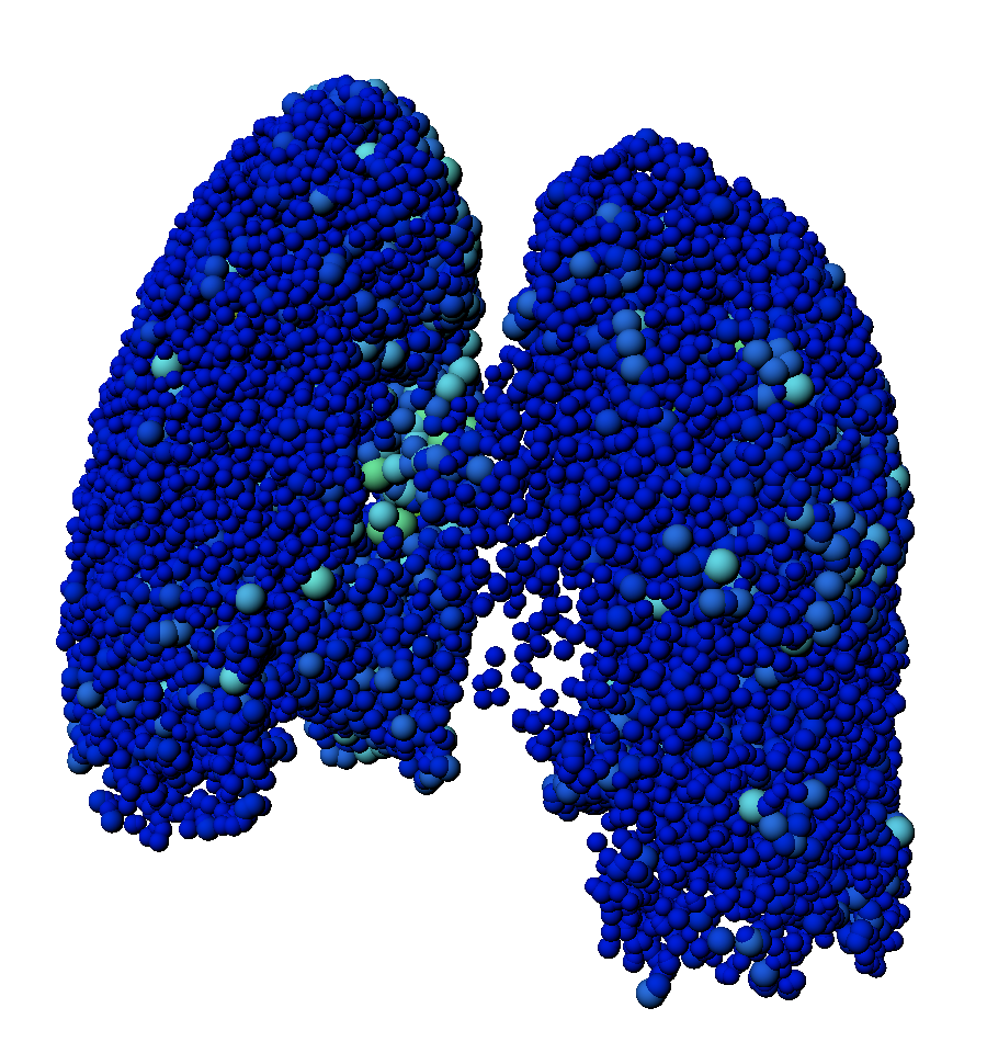
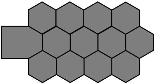
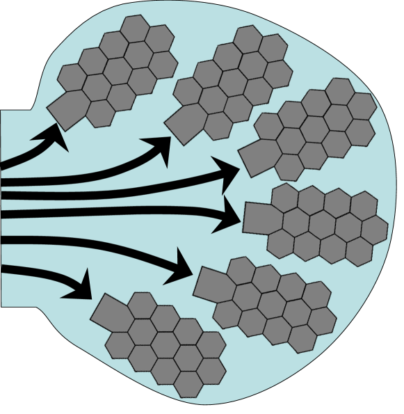
a        b alveolar duct: alveolar cluster:        c

Figure 2: Alveolar cluster model. a Illustrative example of the full cloud of approx. 18,000 alveolar cluster elements used for subject H04 in the present work. Each alveolar cluster is depicted as a sphere with a volume equivalent to the gas volume extracted from the CT image and is colored by that volume. b Schematic of an alveolar duct and a grouping of them forming an alveolar cluster. Image adapted from (5). c Four element Maxwell model of an alveolar duct, with acinar pressure $P_{\mathrm{a}}$, pleural/inter-acinar pressure $P_{\mathrm{pl/intr}}$, and flow rate $Q_{i}$.

2.2.3 Pleurae, chest wall and diaphragm

Elastic recoil of the chest wall and diaphragm as well as gravitational forces are accounted for by means of a suitable external pressure boundary condition acting on the alveolar clusters. This pressure boundary condition therefore depends on the current volume of the lung model as it induces the elastic recoil of the chest wall. The condition also encompasses a hydrostatic pressure component that depends on the weight of the lungs as determined from the CT image by means of a density and volume analysis. Further algorithmic details regarding all aspects of the simulation methodology as well as some recent extensions can be found in (5, 8, 16).

2.3 Particle transport and deposition model

We developed a novel one-way coupled approach to compute particle transport and deposition throughout the entire lungs that hinges on the combination of two novel algorithmic components. First, the computation of particle transport and deposition in reduced-dimensional airways in a Lagrangian fashion through reconstruction of the forces on the particle from the transient reduced-dimensional flow field, and second, a novel approach to combine many pre-computed local-scale 3D CFPD models into a surrogate model that enables the efficient simulation of particle transport across (reduced-dimensional) airway bifurcations. This unique approach enables the tracking of all particles from their seeding in the trachea to the respiratory zone during inhalation as well as exhalation and, for the first time, allows the prediction of aerosol deposition throughout the lungs at sub-millimeter scale. To account for the particle deposition in the mouth-throat region, we have implemented an analytical filter model according to (17). While this simple analytical filter model has been shown to agree very well with state-of-the-art 3D CFPD simulations (18), this part of our modeling approach can also be readily replaced with a patient-specific 3D CFPD model of the upper airways in future works. Due to the focus on the novel whole lung model in this paper and the excellent validation results obtained already with this simple analytical filter model, we decided to leave this extension for future work.

The particles are modeled as point masses with spherical shape. To simulate particle transport, we consider gravitational forces, flow resistance forces according to Reynolds, and a buoyancy force due to density differences between the particle and the fluid as external forces in Newton’s second law of motion. The resulting system of ordinary differential equations are solved using an explicit Forward-Euler time integration scheme. To compute the forces on the particles resulting from the fluid flow, we leverage the instationary, reduced-dimensional flow field obtained from the patient-specific flow simulations to reconstruct the 3D fluid velocity field within each airway element. This results in a velocity field which is transient in the amplitude, but steady in the profile across and along a single airway element for each time step. An example for the parabolic flow velocity field at one cross-section ${v}_{\text{fluid}}$ is shown in Fig. 3 (right side).

Figure 3: Particle transport across airway bifurcations. Left: Schematic showing the creation of the particle transfer database based on a large number of three-dimensional computational fluid and particle dynamics (3D CFPD) simulations covering a large variety of airway geometries, flow regimes, and particle properties. Right: Schematic showing a single reduced-dimensional airway bifurcation where first the particle exit position within the last cross-section of the parent airway (blue) is determined, second the pre-computed result of this particle transfer (green) is retrieved from the database, and finally the particle is transferred to this location within the first cross-section of the daughter airway.

Particle transport across airway bifurcations is computed using an interpolating surrogate model that is based on pre-computed local-scale 3D CFPD simulations of a representative airway bifurcation library. Briefly, we conduct 3D flow simulations for a large library of airways bifurcations accounting for various flow regimes and geometries and subsequently simulate particle transport and deposition within these flow fields, again accounting for variations in a number of parameters such as particle density, size, as well as seeding location. The behavior of particles flowing across these airway bifurcations is recorded, analyzed, and condensed into an interpolating surrogate model that is used to compute particle transport across airway bifurcations in the reduced-dimensional model as illustrated in Fig. 3. In the context of this work, the airway bifurcation library has been filled with a total of 315 scenarios, both systematically sampled from a large CT image database and including also the bifurcations from the first three airway generations of the in vivo reference data set from (1).

Particle deposition in the conducting airways is assumed to occur on contact of the particle with the airway wall. In case the particle reaches the respiratory zone and enters an alveolar cluster with a given shape and volume, a deposition location within this alveolar cluster is chosen randomly. Since our model encompasses the complete airway tree and lung tissue, particles never leave the simulation domain and hence our approach, in contrast to most other simulation approaches, can account for exhalation as well. Therefore, particles, which do not get deposited inside the lung, will either be exhaled or stay in motion and can be simulated and tracked over consecutive breath cycles. Moreover, this completeness of the lung model domain allows to state a total mass balance of the inhaled aerosol as exemplified in Fig. LABEL:fig:mass_balance_and_dep_per_airway_gen and in turn enables detailed investigations such as comparing exhalation losses for different breathing patterns to name just one example.

It is important to emphasize that while the computation of the aforementioned bifurcation library is computationally expensive, this computation has only to be done once before it can be used in a variety of scenarios involving, e.g., different particle sizes, lung geometries and pathologies, and inhalation patterns. Moreover, in combination with the reduced-dimensional transport and deposition simulation in the airway, this approach not only offers unprecedented levels of spatiotemporal tracking of particles in the whole airway tree and lung tissue, but is also efficient enough that patient-specific simulations of aerosol transport and deposition is now possible at scale.

2.4 Simulation setup and boundary conditions

The boundary conditions for the flow and particle simulations are straight forward, as they adhere as close as possible to the experimental setup described in (1, 2, 3, 4) and summarized in SI Sec. 1. In the following the concrete conditions and simplifications are presented for the flow simulation and the one-way coupled particle simulation in turn.

2.4.1 Flow simulation boundary conditions

The respiratory system, as well as our simulation model of the lung, is composed of upper airways, lower airways, and respiratory zone, which are partially enclosed in a chest cavity. The upper airways are omitted from the flow simulations, as the transport of particles through the upper airways is realized through an analytical filter model (17) instead (see SI Sec. 22.2 and 22.3 for details). All flow inlet boundary conditions are hence applied directly to the beginning of the trachea as can be seen in the supplementary videos.

In principle the lung model supports the simulation of spontaneous breathing by applying environmental pressure to the trachea and prescribing the chest cavities expansion and contraction through the volume directly or indirectly through the force of the muscles during breathing. However, for the experiments we are reproducing, an AKITA device has been employed for enforcing a specific flow rate over time (3). This makes the simulation setup analog to that of mechanically ventilated patients for which the flow rate at the trachea is applied also. No additional boundary conditions are needed in this case, as the inflation of the lung/alveolar clusters and the chest cavity, coupled through the pleural pressure, exert counteracting forces (see SI Sec. 22.2 for details). The magnitude of these forces depends on the material properties of the alveolar cluster elements and chest wall and is described in SI Sec. 22.5.

The prescribed inhalation and exhalation flow rates are constructed from two regularized constant flow rates, as shown in Fig. 4.

a     b

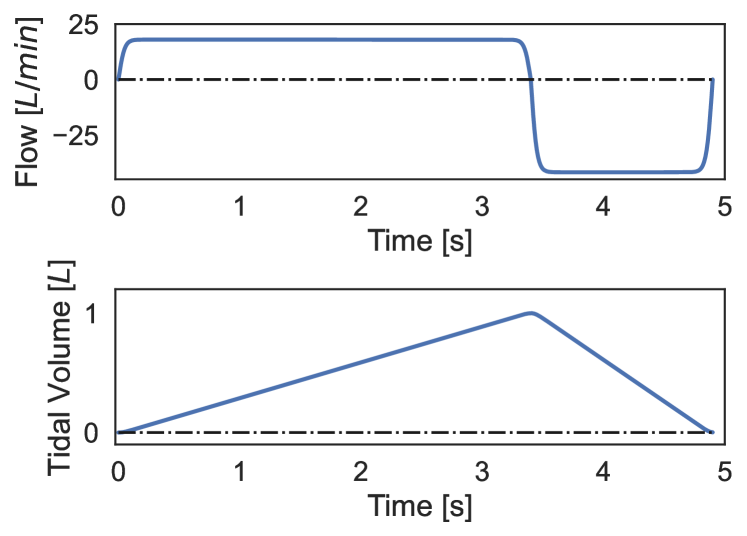
Figure 4: Breathing patterns. Two different breathing patterns applied as flow rate boundary conditions in the simulations, closely following the setup of the experimental study (see (1) and the summary in SI Sec. 1). a Shallow breathing with $600\text{\,}\mathrm{mL}$ tidal volume. b Deep breathing with $1000\text{\,}\mathrm{mL}$ tidal volume.

The inhalation part of the profile represents an idealized AKITA device, that applies a constant flow rate of $18\text{\,}\mathrm{L}\mathrm{/}\mathrm{min}$ (3) to the trachea. Depending on which of the two cases is simulated (see Table 1), the inflow is applied for $2.08\text{\,}\mathrm{s}$ up to $600\text{\,}\mathrm{mL}$ tidal volume or for $3.41\text{\,}\mathrm{s}$ up to $1000\text{\,}\mathrm{mL}$ tidal volume. In either case the first and last $0.4\text{\,}\mathrm{s}$ are regularized with a sigmoid to approximate the natural, smooth increase/decrease from/to zero flow and avoid unphysiological pressure peaks within the lung. In the experiments the forced inhalation is followed up by a breath hold and exhalation that are done within certain time bounds, but at the patients discretion. Diagrams in (1) indicate approximately constant exhalation rates and also some exhalation during the short breath hold phase that was needed to allow the study participants to switch from inhalation device to exhalation device, but is not considered to have a noticeable influence on deposition results. Hence the breath hold and exhalation are subsumed under a single constant outflow rate with regularization for the simulated exhalation phase. In (1) timings are provided for the exhalation phases at the two tidal volumes. Averaging within each group leads to a simulated exhalation duration of $1.27\text{\,}\mathrm{s}$ at $\sim 500\text{\,}\mathrm{m}\mathrm{L}\mathrm{/}\mathrm{s}$ and $1.50\text{\,}\mathrm{s}$ at $\sim 700\text{\,}\mathrm{m}\mathrm{L}\mathrm{/}\mathrm{s}$ for $600\text{\,}\mathrm{mL}$ and $1000\text{\,}\mathrm{mL}$ tidal volume respectively. A pressure increase and later decrease at the trachea inlet arises automatically from the lung tissue and chest cavity counteracting the expansion. However, as the particle transport is driven mostly by the flow velocity, the pressure gradients along the airways are considered to not impact the particle deposition, at least at these low pressure levels.

2.4.2 Particle transport simulation boundary conditions

As for the flow simulation, the boundary conditions to the particle transport simulation strive to reproduce the experiments from (1) and summarized in SI Sec. 1 as close as possible. Hence the particles are seeded statistically over time into the flow during inhalation. The distribution of particle sizes seeded in the simulation matches the MMAD and GSD as provided in Table 1 of (2). Before injection into the trachea however, the particles are filtered through an analytical filter function (17) to account for the deposition in the upper airways (see SI Sec. 22.3 for details). The resulting particle size distributions for a large and a small aerosol size are shown in Fig. 5.

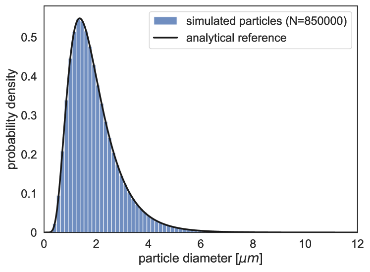
a     b

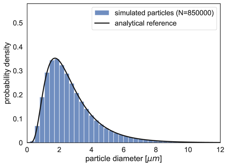
Figure 5: Aerosol particle sizes. Two different aerosol particle size distributions used for the particle simulations (blue), reproducing exactly the setup and measurements of the experimental study cases (see (1) and the summary in SI Sec. 1). For comparison, the analytical reference defined as a log-normal distribution with matching mass median aerodynamic diameter (MMAD) and geometric standard deviation (GSD) is plotted as black solid line. a Small aerosol size with MMAD of $3.38\text{\,}\mathrm{\SIUnitSymbolMicro m}$ and GSD of $1.61\text{\,}\mathrm{a}$s specified for case 2B. b Large aerosol size with MMAD of $6.05\text{\,}\mathrm{\SIUnitSymbolMicro m}$ and GSD of $1.75\text{\,}\mathrm{a}$s specified for case 3B.

Comparing the randomly generated sample of particles to the analytical reference of a log-normal distribution with matching MMAD and GSD shows that both are in excellent agreement for the used number of particles $N$. The particles are seeded at a constant rate of 250,000 particles per second during the inhalation phase, thus leading to a total number $N$ of 520,000 and 850,000 particles for the cases with shallow and deep breathing pattern, respectively. Refer to Table 1 for an overview of the setup used for each of the ten cases. The particles are released into the flow uniform over the area of a plane at the beginning of and perpendicular to the trachea. This emulates the mixing of the particle jet from the glottis by the turbulence within the trachea, but which is not resolved by the reduced-dimensional flow.

2.5 (Material) parameter determination and calibration

The patient specific lung models must be armed with a broad set of material and algorithmic parameters. The source of these parameters range from calibration using patient individual measurements to population average from literature, mainly depending on the availability of data and the underlying modeling assumptions.

2.5.1 Reduced-dimensional whole lung model

Determining patient specific material parameters for the reduced-dimensional lung model is challenging due to the large number of components that make up the human respiratory system and their tight interactions. Naturally, the model should be limited in it’s complexity to the problem it is intended to solve, which is the accurate description of flow distribution in this case. The particle deposition is considered to be driven primarily by the flow velocity distribution, which in turn depends primarily on the individual lung and airway tree geometry and much less on the constitutive behavior. Due to the healthy and homogenous state of the lungs in the conducted validation study, the distribution of stress, strain, and therefore also flow to the alveolar clusters is uniform within the tidal volumes prescribed by the experiments. We expect that the actual levels of stress and strain become important for checking the internal consistency and the application to extreme inhalation maneuvers or patients with lung pathologies. The latter is briefly outlined in the section on Tissue disease modeling of the main text, but not relevant for the healthy subjects of the validation study. For the following fitting procedure of the material parameters to the experimental measurements a steady single compartment version (growth stopped after first generation) of the lung model introduced in SI Sec. 22.1 is assumed, from which the properties are then distributed to the whole lung model. The system of equations for the single compartment is solved under the following series of conditions. The first data point is the CT into which the model is grown and that corresponds to a mean tidal breath-hold (1). The gas volume within the lungs at that state is recovered from the Hounsfield units ($\mathrm{HU}$) assigned to the CT voxel within the lung mask, which are taken as a binary mixture of tissue ($0\text{\,}\mathrm{HU}$) and gas ($-1000\text{\,}\mathrm{HU}$) (19). The next data point is the functional residual capacity (FRC) that was measured in a standing position for every participant. As the FRC is approximately $40\text{\,}\mathrm{\char 37\relax}$ larger in a standing rather than a supine position (20), the FRC in the supine position of the CT can be approximated. In the relaxed state at FRC there is an equilibrium between contractile forces of lung tissue and tensile forces of the chest cavity which results in a negative pressure in the pleural cavity (21). For this mean pleural pressure typically a range of $-3$ to $-5\text{\,}\mathrm{cmH_{2}O}$ is stated in literature, with one concrete measurement at $-4.11\text{\,}\mathrm{cmH_{2}O}$ (22, 23). The mean pleural pressure is further supplemented by a spatially varying component that accounts for gravity through a linear hydrostatic pressure profile over the height dimension, determined from the individual’s average lung density and thus weight. The specific elastance of the lung is taken as $13.8\text{\,}\mathrm{cmH_{2}O}$, which is an average of the non-ARDS cases published in (24). The damping element of the Kelvin-Voigt model is assigned a viscosity of $32.9\text{\,}\mathrm{cmH_{2}O}\mathrm{s}\mathrm{/}\mathrm{L}$ following (9, 5). Another contribution to the overall stiffness of the respiratory system is the chest cavity, comprised of chest wall and diaphragm with abdomen. They are subsumed under a single chest wall elastance, which is determined through the lung elastance to total respiratory elastance ratio. This ratio was approximated at $0.71$ for non-ARDS patients in the measurements provided by (24). The specific chest wall elastance is then $5.7\text{\,}\mathrm{cmH_{2}O}$. With the conditions specified above, the single compartment surrogate of the whole lung model can be solved for the volume of the lungs and chest cavity in a (fictitious) stress free state. They are essential in specifying the patient specific stress strain relationship. The lung model parameters determined so far apply to a patient in supine position. However, the inhalation experiments were carried out in an erect position. Under the simplifying assumption that the change in position only affects the chest cavity’s behavior, the FRC measured for standing study participants can be used to determine a new system state (1). As the difference between supine and erect positions is a change in the direction of the constant gravitational pull, the change in the chest wall condition is taken to be a constant force term as well. Solving for this constant offset in the pleural pressure, a patient specific, standing adjusted specific elastance and stress-free reference volume of the chest cavity is obtained.

2.5.2 Gas and particle characteristics

A further required set of parameters for solving the flow problem in the human lungs are the gas and particle properties. Particles are considered to be spherical droplets of an aquaeous solution. The flow medium is air in an incompressible regime at a density of $1.18\text{\,}\mathrm{k}\mathrm{g}\mathrm{/}\mathrm{m}^{3}$ and dynamic viscosity of $17.9\text{\times}{10}^{-8}\text{\,}\mathrm{cmH_{2}O}\mathrm{/}\mathrm{s}$ in accordance with (9). The effects of a temperature or humidity increase are not accounted for.

3 Additional information on post-processing and data analysis

The main output of the simulation model described in the previous sections are the spatially resolved flow and pressure distribution throughout the lungs as well as the precise location and velocity of each aerosol particle, all in a temporally highly resolved manner. While the former two can be used to derive space and time-dependent ventilation and strain maps, the latter can be used to gauge and quantify aerosol deposition throughout the entire lungs at an unprecedented spatial resolution. The ability to track every single particle trajectory over time even allows to study the dynamics of aerosol transport and deposition over the course of a breath cycle for example, which goes far beyond the usual assessment of the final deposition pattern after finishing the inhalation. Although it is not used in the current validation study due to the lack of in vivo reference data, we would like to emphasize this new opportunity and showcase the high temporal resolution of the simulation result data in the videos provided as supplementary electronic files in Videos 6–6.

3.1 Deposition fraction per lung and per lobe

On the simulation side, the precise deposition location of every particle is known, so using the segmentation masks for the left/right lung and each lobe, it is straightforward to compute the fraction of aerosol mass deposited in each of these sub-domains. On the experimental side, however, we have to deal with the fact that the high-resolution CT (HRCT) image and the SPECT/CT image are not aligned, and in turn also the segmentation masks obtained from the CT image are not directly applicable to the SPECT/CT image data. Hence, to be able to compute deposition fractions from the SPECT/CT images, we first aligned the HRCT image and SPECT/CT image using deformable image registration techniques. Using these deposition fractions from the SPECT/CT images as a reference, we were able to validate the predicted deposition fractions from the simulation by means of direct comparison, correlation analysis or suitable error metrics (see SI Sec. 33.5 for details).

3.2 Central versus peripheral deposition

Analyzing the deposition fraction in peripheral versus central parts of the lungs is commonly used to gauge the fraction of particles that end up in smaller, high-generation airways and the respiratory zone as compared to those depositing in the larger airways. We followed the approach described in (25, 26, 27) to divide the lungs into ten concentric shells and to consider the five inner shells as the central region and the five outer shells as the peripheral region. This is done individually for the left and the right lung, such that we end up with four spatial regions (left-central, left-peripheral, right-central, right-peripheral) that can again be used to validate the predicted deposition fractions against the in vivo reference data from the SPECT/CT image as described for lobar deposition fractions in the previous section. See Fig. LABEL:fig:cp_depositiona for a 3D visualization of the four regions obtained for subject H04.

3.3 Deposition in conducting airways versus respiratory zone

The simulation results allow the direct assessment of the fraction of aerosol mass deposited in the conducting airways as compared to the respiratory zone. This is not possible for the in vivo reference data due to the limited spatial resolution of SPECT/CT and even HRCT images. Therefore, we used the 24h clearance obtained from scintigraphy as a proxy for the conducting airway deposition fraction (CADF) and analyze the correlation with the predicted CADF from the simulation in Fig. LABEL:fig:cadf. To showcase the even higher spatial resolution and result data quality on the simulation side, we also compute the deposition fraction for each generation of the airway tree as shown in Fig. LABEL:fig:mass_balance_and_dep_per_airway_gen.

3.4 Volume normalized deposition fraction

Considering the comparison of deposition in healthy versus diseased parts of the lung, it is necessary to use a volume-normalized deposition fraction, because directly comparing the deposition fractions is inconclusive due to the fact that the two sub-domains (healthy/diseased) differ in size. Therefore, we divide the deposition fraction by the volume fraction of the respective sub-domain in order to get a volume normalized measure that allows to judge the effect of disease on the deposition pattern. Note that this measure is equivalent to a normalized deposition density we obtain from dividing the average deposition density (deposited aerosol mass/volume) in the sub-domain by the average deposition density in the entire domain, i.e., lungs.

3.5 Correlation and error metrics

To quantify the correlation between predicted deposition fractions from simulation and the corresponding reference values from the experimental study, we compute Pearson’s correlation coefficient $\rho$ for all available data points, i.e., every sub-domain and all 10 inhalation experiments. See Figs. LABEL:fig:lobar_depositiond, LABEL:fig:cp_depositiond, LABEL:fig:cadfb, and 6d for the respective number of data points used in the correlation analysis and corresponding scatter plot. To quantify the quality of an individual model prediction, we defined the error as the mass fraction of deposited aerosol that is misattributed to the considered sub-domain, e.g., the lower left lobe for one specific case 4A. On the ensemble level, we use a box-and-whisker plot showing the median (orange line), the range between 25th and 75th percentile (box) and the minimum/maximum value (whiskers) overlaid by a scatter plot showing all individual data points (blue) with some randomly added jitter along the horizontal axis for visibility. See Figs. LABEL:fig:lobar_depositiond, LABEL:fig:cp_depositiond, and 6d for examples.

4 Additional result data

4.1 Validation of predicted deposition fraction per lung

Fig. 6 summarizes the validation results for the predicted aerosol deposition fraction per lung. The analysis and interpretation is analogous to the one for lobar deposition fractions (see Fig. LABEL:fig:lobar_deposition in the main text).

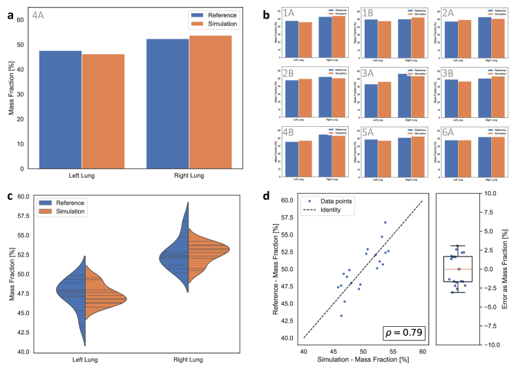
Figure 6: Validation of predicted aerosol deposition per lung. a Deposited aerosol mass as a fraction of total aerosol mass deposited in the lungs. Comparison of model predictions (orange) and in vivo reference data (blue) for subject H04 (visit A). b Comparison of deposition fractions per lung for the remaining 9 inhalation experiments. c Distribution of model predictions (orange) and reference values (blue) for all 10 inhalation experiments (black lines indicate individual cases). d Scatter plot showing correlation and box plot showing error values for all 20 data points (10 inhalation experiments and left/right lung), respectively. The error is defined as the mass fraction of deposited aerosol that is misattributed.

Particle simulation of one full breathing cycle for case 1A. Particle simulation of one full breathing cycle for case 1B. Particle simulation of one full breathing cycle for case 2A. Particle simulation of one full breathing cycle for case 2B. Particle simulation of one full breathing cycle for case 3A. Particle simulation of one full breathing cycle for case 3B. Particle simulation of one full breathing cycle for case 4A. Particle simulation of one full breathing cycle for case 4B. Particle simulation of one full breathing cycle for case 5A. Particle simulation of one full breathing cycle for case 6A.

References

- \bibcommenthead
- (1) Conway, J. et al. Controlled, parametric, individualized, 2-D and 3-D imaging measurements of aerosol deposition in the respiratory tract of healthy human subjects for model validation. Journal of Aerosol Science 52, 1–17 (2012).
- (2) Katz, I. et al. Controlled, Parametric, Individualized, 2D, and 3D Imaging Measurements of Aerosol Deposition in the Respiratory Tract of Healthy Human Subjects: Preliminary Comparisons with Simulations. Aerosol Science and Technology 47, 714–723 (2013).
- (3) Majoral, C. et al. Controlled, Parametric, Individualized, 2D and 3D Imaging Measurements of Aerosol Deposition in the Respiratory Tract of Healthy Human Volunteers: In Vivo Data Analysis. Journal of Aerosol Medicine and Pulmonary Drug Delivery 27, 349–362 (2014).
- (4) Fleming, J. et al. Controlled, Parametric, Individualized, 2-D and 3-D Imaging Measurements of Aerosol Deposition in the Respiratory Tract of Asthmatic Human Subjects for Model Validation. Journal of Aerosol Medicine and Pulmonary Drug Delivery 28, 432–451 (2015).
- (5) Ismail, M., Comerford, A. & Wall, W. A. Coupled and reduced dimensional modeling of respiratory mechanics during spontaneous breathing. International Journal for Numerical Methods in Biomedical Engineering 29, 1285–1305 (2013).
- (6) Tawhai, M. H., Pullan, A. J. & Hunter, P. J. Generation of an anatomically based three-dimensional model of the conducting airways. Annals of Biomedical Engineering 28, 793–802 (2000).
- (7) Roth, C. J., Ismail, M., Yoshihara, L. & Wall, W. A. A comprehensive computational human lung model incorporating inter-acinar dependencies: Application to spontaneous breathing and mechanical ventilation. International Journal for Numerical Methods in Biomedical Engineering 33, e02787 (2017).
- (8) Roth, C. J., Yoshihara, L., Ismail, M. & Wall, W. A. Computational modelling of the respiratory system: Discussion of coupled modelling approaches and two recent extensions. Computer Methods in Applied Mechanics and Engineering 314, 473–493 (2017).
- (9) Roth, C. J., Becher, T., Frerichs, I., Weiler, N. & Wall, W. A. Coupling of EIT with computational lung modeling for predicting patient-specific ventilatory responses. Journal of Applied Physiology 122, 855–867 (2017).
- (10) Alastruey, J., Parker, K. H. & Peiró, J. Lumped parameter outflow models for 1-D blood flow simulations: Effect on pulse waves and parameter estimation. Communications in Computational Physics 4, 317–336 (2008).
- (11) Pedley, T. J., Schroter, R. C. & Sudlow, M. F. The prediction of pressure drop and variation of resistance within the human bronchial airways. Respiration physiology 9, 387–405 (1970).
- (12) van Ertbruggen, C., Hirsch, C. & Paiva, M. Anatomically based three-dimensional model of airways to simulate flow and particle transport using computational fluid dynamics. Journal of Applied Physiology 98, 970–980 (2005).
- (13) Bel-Brunon, A., Kehl, S., Martin, C., Uhlig, S. & Wall, W. Numerical identification method for the non-linear viscoelastic compressible behavior of soft tissue using uniaxial tensile tests and image registration – Application to rat lung parenchyma. Journal of the Mechanical Behavior of Biomedical Materials 29, 360–374 (2014).
- (14) Rausch, S. M. K., Martin, C., Bornemann, P. B., Uhlig, S. & Wall, W. A. Material model of lung parenchyma based on living precision-cut lung slice testing. Journal of the Mechanical Behavior of Biomedical Materials 4, 583–592 (2011).
- (15) Birzle, A. M., Hobrack, S. M. K., Martin, C., Uhlig, S. & Wall, W. A. Constituent-specific material behavior of soft biological tissue: Experimental quantification and numerical identification for lung parenchyma. Biomechanics and Modeling in Mechanobiology 18, 1383–1400 (2019).
- (16) Geitner, C. M. et al. An approach to study recruitment/derecruitment dynamics in a patient-specific computational model of an injured human lung (2022).
- (17) Stahlhofen, W., Rudolf, G. & James, A. Intercomparison of Experimental Regional Aerosol Deposition Data. Journal of Aerosol Medicine 2, 285–308 (1989).
- (18) Borojeni, A. A. T. et al. In Silico Quantification of Intersubject Variability on Aerosol Deposition in the Oral Airway. Pharmaceutics 15, 160 (2023).
- (19) Gattinoni, L., Caironi, P., Pelosi, P. & Goodman, L. R. What Has Computed Tomography Taught Us about the Acute Respiratory Distress Syndrome? American Journal of Respiratory and Critical Care Medicine 164, 1701–1711 (2001).
- (20) Ibañez, J. & Raurich, J. M. Normal values of functional residual capacity in the sitting and supine positions. Intensive Care Medicine 8, 173–177 (1982).
- (21) Gattinoni, L. et al. Targeting transpulmonary pressure to prevent ventilator-induced lung injury. Expert Review of Respiratory Medicine 13, 737–746 (2019).
- (22) Zielinska-Krawczyk, M., Krenke, R., Grabczak, E. M. & Light, R. W. Pleural manometry–historical background, rationale for use and methods of measurement. Respiratory Medicine 136, 21–28 (2018).
- (23) Aron, E. Der intrapleurale Druck beim lebenden, gesunden Menschen. Archiv für pathologische Anatomie und Physiologie und für klinische Medicin 160, 226–234 (1900).
- (24) Chiumello, D. et al. Lung Stress and Strain during Mechanical Ventilation for Acute Respiratory Distress Syndrome. American Journal of Respiratory and Critical Care Medicine 178, 346–355 (2008).
- (25) Perring, S., Summers, Q., Fleming, J. S., Nassim, M. A. & Holgate, S. T. A new method of quantification of the pulmonary regional distribution of aerosols using combined CT and SPECT and its application to nedocromil sodium administered by metered dose inhaler. The British Journal of Radiology 67, 46–53 (1994).
- (26) Fleming, J. S., Sauret, V., Conway, J. H. & Martonen, T. B. Validation of the Conceptual Anatomical Model of the Lung Airway. Journal of Aerosol Medicine 17, 260–269 (2004).
- (27) Fleming, J. S., Epps, B. P., Conway, J. H. & Martonen, T. B. Comparison of SPECT Aerosol Deposition Data with a Human Respiratory Tract Model. Journal of Aerosol Medicine 19, 268–278 (2006).