Do pulsar timing arrays observe merging primordial black holes?

Abstract

In this letter we evaluate whether the gravitational wave background recently observed by a number of different pulsar timing arrays could be due to merging primordial supermassive black hole binaries. We find that for homogeneously distributed primordial black holes this possibility is inconsistent with strong cosmological and astrophysical constraints on their total abundance. If the distribution exhibits some clustering, however, the merger rate will in general be enhanced, opening the window for a consistent interpretation of the PTA data in terms of merging primordial black holes.

Introduction.—

The discovery of gravitational waves (GWs) with frequencies $\mathcal{O}(100)\,\mathrm{Hz}$ from binary black hole mergers in 2015 [1] has opened new possibilities for the exploration of our Universe. Depending on the astrophysical or cosmological source, GW signals may exist over a wide range of frequencies and complementary experimental approaches aim to explore much of the available parameter space [2, 3]. Pulsar timing arrays (PTAs) in particular are sensitive at frequencies in the nHz range. In 2020 NANOGrav [3] announced evidence for a common red process hinting at a stochastic nHz gravitational wave background (GWB), with similar results subsequently published by other PTAs [4, 5, 6]. Excitingly, the very recent data releases from NANOGrav [7], EPTA [8], PPTA [9], and CPTA [10] not only strengthen this signal, but also show mounting evidence for the characteristic quadrupolar Hellings-Downs correlation [11]. It is therefore fascinating and timely to investigate possible origins of this newly observed signal in terms of a GWB. Mergers of supermassive black hole binaries (SMBHB) are expected to contribute to the GWB in this frequency range [3], although the local SMBHB density would need to be $\mathcal{O}(10)$ larger than previously estimated [12, 13, 14] to match the observed signal amplitude. Hence, the validity of this explanation is under active debate [15, 16, 17, 18] and it is interesting to consider alternative sources. A nHz GWB could also originate from truly cosmological sources [19, 20], such as inflation [21], topological defects [22, 23, 24, 25, 26, 27], first-order phase transitions [28, 29, 30, 31, 32], or the production of sub-solar mass primordial black holes (PBHs) [33, 34, 35, 36, 37].

In this letter we study the possibility that the observed GW signal could be due to merging supermassive PBH binaries. To obtain the correct signal amplitude, a sizeable abundance of PBHs is required, which is subject to strong constraints from various observational probes [38]. It is therefore a non-trivial question as to whether merging PBHs could constitute a viable explanation. Indeed we find that it is not possible to consistently explain the NANOGrav data with homogeneously distributed PBHs. Specifically the parameter regions at very large PBH masses which naively allow to fit the PTA data (as done in [39]) no longer result in a stochastic (or even continuous) signal. For clustered PBHs, on the other hand, the formation of binary systems is more efficient and the merger rate is generally enhanced, opening the possibility for an overall consistent description of the observed GWB.

This letter is structured as follows. We first review and extend the formalism required to evaluate the GWs from binary mergers for the case of clustered PBHs. After discussing the relevant constraints and how to match the predicted signal to PTA data we present our results.

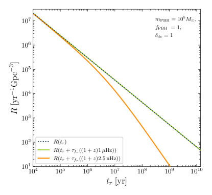
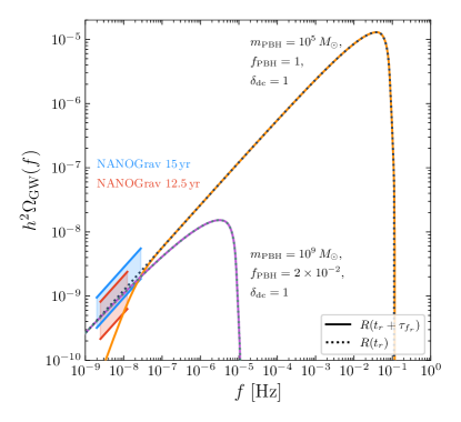
Figure 1: Left: Rate for binaries merging at $t_{\text{r}}$ (dotted line) as well as rate for emitting GWs at $t_{\text{r}}$ with different frequencies today (solid green and orange lines). Right: GW energy density $h^{2}\Omega_{\text{GW}}(f)$ obtained using the correct rate $R(t_{\text{r}}+\tau_{f_{\text{r}}})$ (solid lines) and instead using the merger rate $R(t_{\text{r}})$ in Eq. (2) (dotted lines). We also show the regions of the NANOGrav 12.5 yr and 15 yr signals assuming the inspiral of binary BHs.

Gravitational wave signal.—

A stochastic GWB can be specified in terms of the energy density parameter $h^{2}\Omega_{\mathrm{GW}}(f)$ of GWs per logarithmic frequency interval around a frequency $f$. In our scenario, this GWB is generated from PBH binary mergers occurring at a rate $R(t_{\text{r}})$ per comoving volume $V_{\text{c}}$ and cosmic time $t_{\text{r}}$ . The frequencies accessible to PTAs can be well below the maximal frequency emitted during the merger and might therefore have been radiated long before coalescence, which we need to take into account. In particular, a given binary merging at time $t_{r,\text{merg}}$ has emitted a frequency $f_{\text{r}}$ in the cosmic rest frame, redshifted to a frequency $f=f_{\text{r}}/(1+z)$ today, at time $t_{\text{r}}=t_{r,\text{merg}}-\tau_{f_{\text{r}}}$, where

$$\tau_{f_{\text{r}}}=\frac{5\times 2^{1/3}}{256\,\pi^{8/3}}\,f_{\text{r}}^{-8/3}\,(G\,m_{\mathrm{PBH}})^{-5/3}$$ (1)

is the time until coalescence for $f_{\text{r}}$ [40]. As $t_{r,\text{merg}}$ is the argument for the merger rate, the number of events per comoving volume and cosmic time emitting a frequency $f_{\text{r}}$ in the cosmic rest frame at cosmic time $t_{\text{r}}$ is given by $R(t_{\text{r}}+\tau_{f_{\text{r}}})$. To the best of our knowledge this frequency-dependent rate has not been discussed yet in the literature concerning GWs generated by PBHs. The GW energy density parameter is given by (cf. [41])

$$\Omega_{\mathrm{GW}}(f)=\frac{f}{\rho_{\mathrm{crit}}}\int_{0}^{t_{0}}\mathrm{d}t_{\text{r}}\left(R(t_{\text{r}}+\tau_{f_{\text{r}}})\frac{\mathrm{d}E_{\mathrm{GW}}}{\mathrm{d}f_{\text{r}}}\right)_{f_{\text{r}}=(1+z)f}\;,$$ (2)

where $t_{0}$ is the current cosmic time and $\mathrm{d}E_{\mathrm{GW}}/\mathrm{d}f_{\text{r}}$ is the GW spectrum, which we adopt from [42]. Note that $h^{2}\Omega_{\mathrm{GW}}(f)$ is in fact a cosmological average of many PBH binaries. We discuss the effect of only having access to a local realisation of the GWB within PTA measurements below.

For the merger rate we adapt the calculation from [43]. We assume a monochromatic initial PBH mass distribution, expecting that an extended distribution does not qualitatively change our results. A PBH binary forms in the early Universe when the gravitational attraction between two neighbouring PBHs overcomes the Hubble flow. A third close-by PBH provides angular momentum such that the two PBHs do not simply collide [44, 45, 46].

Clearly the merger rate depends on the local PBH density at binary formation. It is therefore interesting to study the effect of clustering, which increases the local density by $\delta_{\mathrm{dc}}$ compared to the global comoving number density $n_{\mathrm{PBH}}$. The density contrast $\delta_{\mathrm{dc}}$ can be considered constant on the scales relevant for binary formation [43]. By considering the number density of three-body configurations relevant for PBH binary formation and their coalescence times (in terms of the distances in the three-body configurations) [48, 43] one finds [43]

$$R(t_{\text{r}})=\frac{9\,\tilde{N}^{53/37}_{\mathrm{PBH}}}{296\pi\,\delta_{\mathrm{dc}}\,\tilde{x}^{3}\,\tilde{\tau}}\left(\frac{t_{\text{r}}}{\tilde{\tau}}\right)^{-34/37}\times$$

$$\!\left(\Gamma\left[\frac{58}{37},\tilde{N}_{\mathrm{PBH}}\left(\frac{t_{\text{r}}}{\tilde{\tau}}\right)^{3/16}\right]\!\!-\!\Gamma\left[\frac{58}{37},\tilde{N}_{\mathrm{PBH}}\left(\frac{t_{\text{r}}}{\tilde{\tau}}\right)^{-1/7}\right]\right)$$ (3)

with $\tilde{x}=3\,m_{\mathrm{PBH}}/(8\pi\,a_{\mathrm{eq}}^{3}\,\rho_{\mathrm{eq}})$, the scale factor $a_{\mathrm{eq}}$ and energy density $\rho_{\mathrm{eq}}$ at matter-radiation equality [49], $\tilde{\tau}=3\,(a_{\mathrm{eq}}\,\tilde{x})^{4}/[170\,(G\,m_{\mathrm{PBH}})^{3}]$, $\tilde{N}_{\mathrm{PBH}}=4\pi\,n_{\mathrm{PBH}}\,\delta_{\mathrm{dc}}\,\tilde{x}^{3}/3$, and the incomplete gamma function $\Gamma$.

Larger clustering generally leads to a larger number of PBH binaries contributing to the merger rate (note that $\tilde{N}_{\mathrm{PBH}}\propto\delta_{\mathrm{dc}}$) as well as a shorter timescale for the mergers (cf. the arguments of the gamma functions). Furthermore, multiple merger steps can be possible for large clustering due to successive hierarchical merging of PBH binaries with increasing mass. When discussing the case of significant clustering we implement multiple merger steps by adding the rates and contributions to the GW energy density parameter for the corresponding steps as detailed in [50]. Note that this slightly shifts our results for significant clustering to lower PBH abundances compared to only considering a single step.

By substituting $t_{\text{r}}\rightarrow t_{\text{r}}+\tau_{f_{\text{r}}}$ in Eq. (3) we can compute the rate $R(t_{\text{r}}+\tau_{f_{\text{r}}})$ for the emission of a frequency $f_{\text{r}}$. To illustrate the importance of the emission time of a given frequency, in Fig. 1 (left) we compare the rate for binaries merging at $t_{\text{r}}$ (dotted blue line) with the rate for GW emission with frequencies $f=1\,\mu\mathrm{Hz}$ and $2.5\,\mathrm{nHz}$ today (solid green and orange lines), assuming a PBH mass $m_{\mathrm{PBH}}=10^{5}\,M_{\odot}$, a fraction $f_{\mathrm{PBH}}=1$ of dark matter (DM) in PBHs, and $\delta_{\mathrm{dc}}=1$. For instance, at $t_{\text{r}}=10^{8}\,\mathrm{yr}$ (i.e. $z\approx 30$) one obtains $\tau_{f_{\text{r}}}((1+z)1\,\mu\mathrm{Hz})\approx 130\,\mathrm{yr}$ and $\tau_{f_{\text{r}}}((1+z)2.5\,\mathrm{nHz})\approx 1.1\times 10^{9}\,\mathrm{yr}$. Hence, the rate for the emission of GWs with the larger frequency (solid green line) is very close to the merger rate (dotted blue line), whereas the rate for the emission of GWs with the smaller frequency (solid orange line) differs significantly, i.e. it takes the value that the dotted blue line attains $1.1\times 10^{9}\,\mathrm{yr}$ later.

In the right panel of Fig. 1 we show $h^{2}\Omega_{\mathrm{GW}}(f)$ according to Eq. (2) (solid lines) as well as just inserting the merger rate $R(t_{\text{r}})$ instead of $R(t_{\text{r}}+\tau_{f_{\text{r}}})$ in the integral (dotted lines). The difference between those calculations is especially important for the low frequencies observed by NANOGrav if the PBH mass is relatively light.

We close the discussion of the GWB signal by mentioning some assumptions in the calculation. These include a monochromatic mass distribution [43], a circular orbit of the binaries for the GWB spectrum and the time until coalescence for a given frequency, neglecting the effect of other PBHs on the binaries [51, 52] as well as further environmental effects e.g. due to accretion, and late-time formation of binaries [43]. Apart from the effect of other PBHs on binaries, which can potentially reduce their merger rate [52], but require $N$-body simulations for an accurate treatment that are beyond the scope of this work, these assumptions are not expected to have a qualitative impact on our results.

Expected number of binaries.—

The PTA signals are reported as stochastic GWBs. While there have been searches for signals of individual binaries in the data of different PTAs [53, 54, 55], no compelling evidence for these signals was found. For sufficiently large PBH masses and small abundances the expected signal will in general no longer resemble a stochastic background, as only very few binaries will contribute to the signal, causing inconsistency with observations.

The problem is exacerbated by the question of how well an actual distribution of merging binaries observed by a PTA (corresponding to a local GW energy density $\Omega_{\mathrm{GW},\mathrm{loc}}$ on the length scales relevant for PTAs) would reproduce the global average of the GWB $h^{2}\Omega_{\mathrm{GW}}(f)=h^{2}\langle\Omega_{\mathrm{GW},\mathrm{loc}}(f)\rangle$, i.e. how well the global mean is reproduced by the binaries that are in our past light cone. In particular, $h^{2}\Omega_{\mathrm{GW},\mathrm{loc}}(f)$ is not deterministic given model parameters (mass, abundance, and clustering of PBHs), but instead stochastic in itself. The statistics of $h^{2}\Omega_{\mathrm{GW},\mathrm{loc}}(f)$ can be evaluated using Markov chain Monte Carlo methods or moment generating functions [56]. Due to the considerable additional numerical effort we leave this for future studies, use the global average signal prediction $h^{2}\Omega_{\mathrm{GW}}(f)$, and identify regions in parameter space where we expect a significant deviation from the global average.

Most importantly, the distribution of $h^{2}\Omega_{\mathrm{GW},\mathrm{loc}}(f)$ is influenced by the expected number of binaries $\bar{N}(f_{-},f_{+})$ contributing to the GWB in a frequency range between $f_{-}$ and $f_{+}$. In the appendix we use [57] to show that

$$\bar{N}(f_{-},f_{+})=\!\int_{f_{-}}^{f_{+}}\frac{\mathrm{d}f}{f}\int_{0}^{\infty}\mathrm{d}z\,\frac{32\pi\tau_{f_{\text{r}}}\,[d_{\text{c}}(z)]^{2}}{3H(z)}R(t_{\text{r}}-\tau_{f_{\text{r}}})\;,$$ (4)

where $d_{\text{c}}$ is the comoving distance and $H$ is the Hubble rate. As we fit to the 14 lowest frequencies in the NANOGrav 15 yr data set we use $f_{-}=1/T_{\text{obs}}^{\text{15}}=1.98\,\text{nHz}$ and $f_{+}=14/T_{\text{obs}}^{\text{15}}=27.7\,\text{nHz}$.

If $\bar{N}\gg 1$, many PBH binaries contribute to the GW signal and the local GWB is very close to the global value. This holds even though uncertainties due to some close-by binaries can be relevant for $\bar{N}\lesssim 100$ and can potentially cause spikes in the local GWB [56]. If $\bar{N}\sim\mathcal{O}(\text{few})$, i.e. the GW signal is composed of only a few binaries, the uncertainty in the signal prediction is considerable. It would then be more appropriate to search for individual GW events instead of a GWB [53, 54, 55]. If $\bar{N}\ll 1$, even having a single PBH binary emitting GWs is unlikely and in most realisations $h^{2}\Omega_{\mathrm{GW},\mathrm{loc}}(f)=0$.

PBH production and constraints.—

There are many different production mechanisms for PBHs, see e.g. [58, 59, 60, 61, 62, 63, 64]. Highly clustered PBH distributions in particular are not expected for Gaussian primordial fluctuations [65, 66], but could e.g. arise due to primordial non-Gaussianities [67, 68] or from the collapse of domain walls [59]. In this work we remain agnostic about the origin and spatial distribution of PBHs and concentrate on exploring the phenomenological impact of different assumptions.

Different astrophysical and cosmological observations place constraints on the abundance of heavy PBHs, which we adopt from [38]. These limits assume a monochromatic mass function as well as a roughly homogeneous spatial distribution (no clustering). While we briefly comment on the expected impact of sizeable clustering, a full re-evaluation of these limits would require going beyond some of the simple approximations made in the original derivations and is beyond the scope of this letter. Also note that many of the different constraints come with different uncertainties and sometimes also with additional caveats.

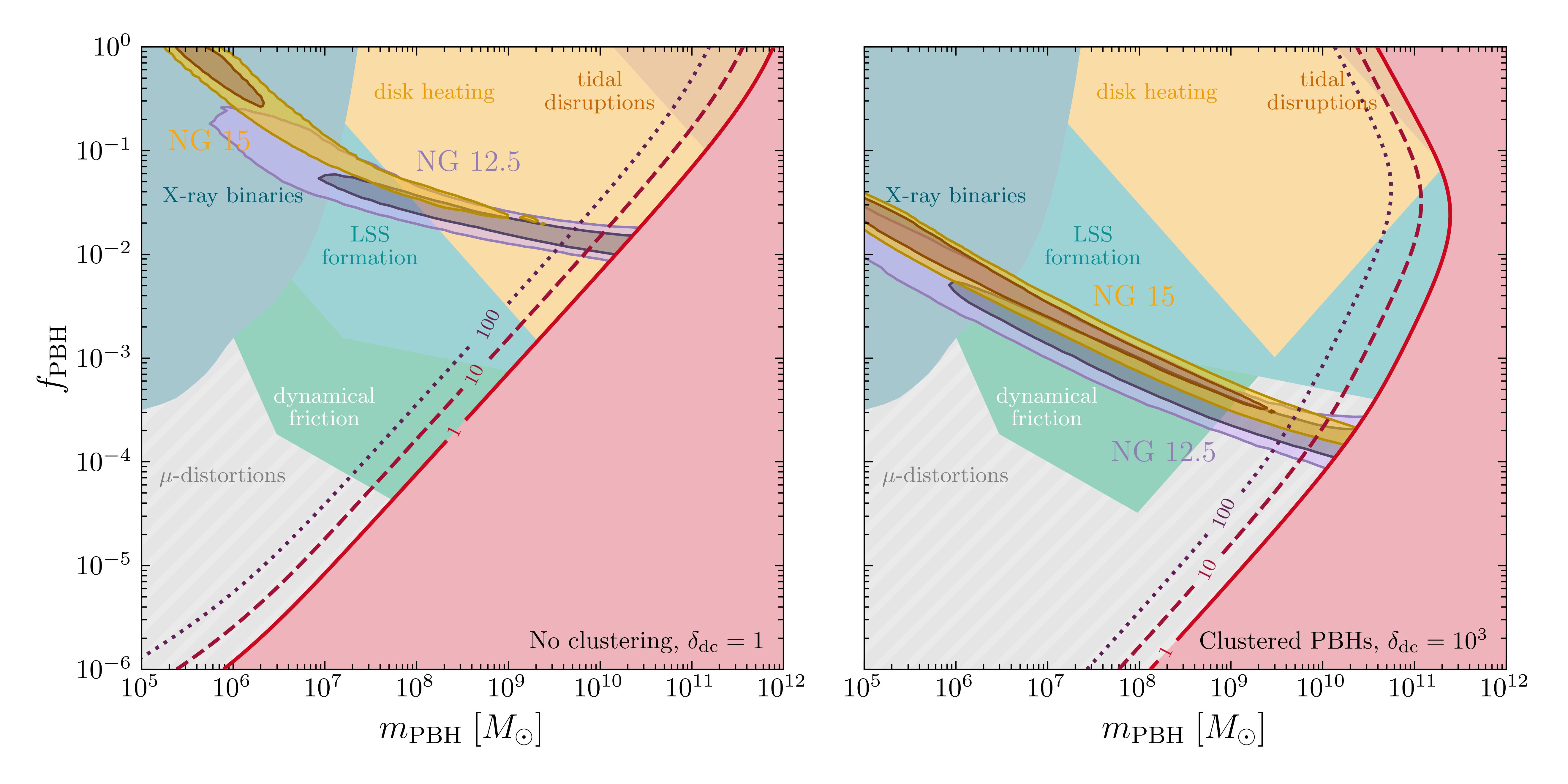
Figure 2: Best-fit region where the NANOGrav 15 yr (brown) and 12.5 yr (purple) data set can be explained by merging PBH binaries without clustering (left) and with significant clustering (right). We indicate regions, where $\bar{N}<1$, $10$, and $100$ PBH binaries are expected to contribute to the signal, and show complementary constraints as discussed in the main text.

The most relevant limits in the mass range of interest come from the heating of stars in the Galactic disk [69], the tidal disruption of galaxies [69], the dynamical friction effect on halo objects [69], requiring successful formation of the observed large scale structure [70], and observations of X-ray binaries [71]. Many of these limits require at least one PBH per relevant cosmic structure. In case of PBH clustering, we expect that some structures will contain more than one PBH while others contain no PBH at all. This will likely weaken a number of limits and move them to smaller masses. A proper evaluation of the PBH spatial distribution and the resulting limits will however require detailed simulations.

Depending on the production mechanism of the PBHs, strong limits may also arise from the observation of the cosmic microwave background (CMB). In particular if PBHs form due to the tail of Gaussian density fluctuations, Silk damping leads to $\mu$-distortions and strong constraints over a sizeable mass range [72]. However, this limit crucially depends on the production mechanism and may therefore even be completely evaded. In fact, as discussed above, large clustering generally requires a different production mechanism, calling into question the relevance of these limits.

PTA data analysis.—

We fit the GWB spectrum from PBH binary mergers to the NANOGrav 15 yr and 12.5 yr data sets via the interface ptarcade [73] for ceffyl [74] using the 14 (five) lowest Fourier modes for the 15 yr (12.5 yr) data set. Given that evidence for a Hellings-Downs correlation is only present in the new data set, we assume a common uncorrelated red noise spectrum for the 12.5 yr data set and only move to Hellings-Downs correlations for the 15 yr data set. We validated our approach by comparison to results obtained using enterprise and enterprise-extensions [75, 76]. We perform calculations with no clustering, $\delta_{\mathrm{dc}}=1$, and significant clustering, $\delta_{\mathrm{dc}}=10^{3}$, choosing log priors $f_{\text{PBH}}\in[10^{-5},1]$ and $m_{\text{PBH}}\in[10^{5},10^{12}]\,M_{\odot}$. When deriving constraints we further add a power-law signal corresponding to SMBHBs. After marginalising over the amplitude, the region in the remaining $(m_{\text{PBH}},f_{\text{PBH}})$ plane excluded with $2\,\sigma$ corresponds to the excluded parameter space in which the expected GWB signal from PBH binaries would exceed observations.

Results.—

In Fig. 2 we show the regions in PBH mass $m_{\mathrm{PBH}}$ and DM fraction $f_{\mathrm{PBH}}$, where the NANOGrav signal can be explained assuming merging PBHs with no clustering (left) and significant clustering with $\delta_{\mathrm{dc}}=10^{3}$ (right). These contours are only expected to be reliable when the expected number of binaries is $\bar{N}\gtrsim 10$ (cf. dashed dark red lines) as otherwise the signal observable in NANOGrav is expected to have significant deviations from the global average GWB signal used in our analysis. Especially for $\bar{N}<1$ (full red line) one would not even expect any GWB signal in most realisations of PBH binary distributions. These effects were neglected in [39] that falsely concluded that the NANOGrav signal could be explained in a region of parameter space without clustering, where $\bar{N}\lesssim 1$. We find that the case without clustering cannot explain the NANOGrav signal once taking into account cosmological and astrophysical constraints.

Including clustering shifts the signal regions to smaller $f_{\mathrm{PBH}}$, enabling a consistent explanation of the PTA data without violating observational constraints, provided that the PBH formation mechanism does not result in significant $\mu$-distortions. Note that clustering is also expected to further open up parameter space for a consistent explanation as complementary constraints are expected to become weaker.

Comparing the results for the 15 yr and 12.5 yr data sets we note that the signal regions have shifted to larger $f_{\mathrm{PBH}}$, due to the preference for a larger GWB in the new data set [3, 7], and there is a slight preference for lower masses, where the earlier emission of GWs leads to an increased slope, cf. Fig. 1, as preferred by the new data [7].

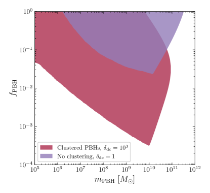
Figure 3: Constraints on PBHs from PTA observations with no clustering (purple) and significant clustering $\delta_{\mathrm{dc}}=10^{3}$ (red). We conservatively cut the limits when the expected number of binaries contributing to the signal falls below $10$.

If the GWB signal generated by merging PBH binaries becomes too large, above the regions explaining the PTA data in Fig. 2, the abundance of PBHs can be constrained by PTA observations. The constraints are shown in Fig. 3 with and without clustering, conservatively requiring $\bar{N}\geq 10$.

Discussion and conclusions.—

In this letter we have studied the possibility that the signal observed by various pulsar timing arrays is due to merging primordial supermassive black hole binaries. If the PBHs are “homogeneously” distributed at their formation, i.e. follow a Poisson distribution, significant cosmological and astrophysical constraints exclude the possibility of explaining the PTA signal with merging PBHs. Instead considering a clustered spatial distribution of PBHs increases the binary merger rate and thus enables a consistent explanation of the PTA signals with merging PBH binaries. Crucially, we have checked that also the signal prediction is reliable in the relevant parameter space by computing the expected number of binaries contributing to the gravitational wave signal. Further, we used PTA data to constrain the PBH parameter space when the GWB generated during the mergers would result in stronger signal strengths than the one detected.

This work may serve as a motivation for model builders to construct scenarios that can generate clustered supermassive PBHs without running into cosmological and astrophysical constraints, in particular due to $\mu$-distortions of the CMB arising from PBH formation. While the latest PTA data finds no evidence for individual compact binary merger events on top of a stochastic background or anisotropies of the GW spectrum, the situation might change in the future. Such a detection would likely invalidate most other cosmological explanations, but is a prediction of our scenario.

Appendix

Expected number of binaries.—

In this appendix we derive the expression for the expected number of primordial black hole binaries contributing to the gravitational wave background within a given frequency range. To do so, recall that $R(t_{\text{r}}+\tau_{f_{\text{r}}})$ is the number of binaries per comoving volume $V_{\text{c}}$ and per time interval in the cosmic rest frame $t_{\text{r}}$ emitting with a frequency $f_{\text{r}}$, where $\tau_{f_{\text{r}}}$ is the time until coalescence. Hence, the expected number of binaries $\mathrm{d}\bar{N}$ emitting at redshifts between $z$ and $z+\mathrm{d}z$ with a frequency within the logarithmic interval $\mathrm{d}\ln f_{\text{r}}$ around $f_{\text{r}}$ is [57]

$$R(t_{\text{r}}+\tau_{f_{\text{r}}}) =\frac{\mathrm{d}z}{\mathrm{d}t_{\text{r}}}\frac{\mathrm{d}^{2}\bar{N}}{\mathrm{d}z\,\mathrm{d}\ln f_{\text{r}}}\frac{\mathrm{d}\ln f_{\text{r}}}{\mathrm{d}t_{\text{r}}}\frac{\mathrm{d}t_{\text{r}}}{\mathrm{d}z}\frac{\mathrm{d}z}{\mathrm{d}V_{\text{c}}}$$

$$=\frac{\mathrm{d}^{2}\bar{N}}{\mathrm{d}z\,\mathrm{d}\ln f_{\text{r}}}\left(-\frac{\mathrm{d}\ln f_{\text{r}}}{\mathrm{d}\tau_{f_{\text{r}}}}\right)\frac{\mathrm{d}z}{\mathrm{d}V_{\text{c}}}\;,$$ (5)

where we used that the time in the cosmic rest frame a source is emitting within the frequency interval is given by

$$\mathrm{d}t_{\text{r}}\frac{\mathrm{d}\ln f_{\text{r}}}{\mathrm{d}t_{\text{r}}}=-\mathrm{d}t_{\text{r}}\frac{\mathrm{d}\ln f_{\text{r}}}{\mathrm{d}\tau_{f_{\text{r}}}}\;.$$ (6)

Since the binaries emitting in the logarithmic frequency interval $\mathrm{d}\ln f_{\text{r}}$ around $f_{\text{r}}$ are detected today in a logarithmic frequency interval $\mathrm{d}\ln f$ around $f$, where $\mathrm{d}\ln f_{\text{r}}=\mathrm{d}f_{\text{r}}/f_{\text{r}}=\mathrm{d}f/f=\mathrm{d}\ln f$, we have

$$\frac{\mathrm{d}^{2}\bar{N}}{\mathrm{d}z\,\mathrm{d}\ln f}=\frac{\mathrm{d}^{2}\bar{N}}{\mathrm{d}z\,\mathrm{d}\ln f_{\text{r}}}\;.$$ (7)

With Eq. (1) from the main text and the definition of the comoving volume in a spatially flat universe

$$V_{\text{c}}(z)=\frac{4\pi}{3}[d_{\text{c}}(z)]^{3}=\frac{4\pi}{3}\left(\int_{0}^{z}\frac{\mathrm{d}z^{\prime}}{H(z^{\prime})}\right)^{3}\;,$$ (8)

where $d_{\text{c}}$ is the comoving distance and $H$ is the Hubble rate, we find

$$\frac{\mathrm{d}^{2}\bar{N}}{\mathrm{d}z\,\mathrm{d}\ln f}=\frac{8}{3}\,\tau_{f_{\text{r}}}\,\frac{4\pi\,[d_{\text{c}}(z)]^{2}}{H(z)}\,R(t_{\text{r}}-\tau_{f_{\text{r}}})\;.$$ (9)

The average number of binaries $\bar{N}(f_{-},f_{+})$ contributing to GWs of frequencies between $f_{-}$ and $f_{+}$ is therefore given by

$$\bar{N}(f_{-},f_{+})=\!\int_{f_{-}}^{f_{+}}\frac{\mathrm{d}f}{f}\int_{0}^{\infty}\mathrm{d}z\,\frac{32\pi\tau_{f_{\text{r}}}\,[d_{\text{c}}(z)]^{2}}{3H(z)}R(t_{\text{r}}-\tau_{f_{\text{r}}})\;.$$ (10)

Note that the actual number of binaries is then Poisson distributed with mean $\bar{N}(f_{-},f_{+})$.

References

- Abbott et al. [2016] B. P. Abbott et al. (LIGO Scientific, Virgo), Observation of Gravitational Waves from a Binary Black Hole Merger, Phys. Rev. Lett. 116, 061102 (2016), arXiv:1602.03837 [gr-qc] .
- Amaro-Seoane et al. [2017] P. Amaro-Seoane et al. (LISA), Laser Interferometer Space Antenna, (2017), arXiv:1702.00786 [astro-ph.IM] .
- Arzoumanian et al. [2020] Z. Arzoumanian et al. (NANOGrav), The NANOGrav 12.5 yr Data Set: Search for an Isotropic Stochastic Gravitational-wave Background, Astrophys. J. Lett. 905, L34 (2020), arXiv:2009.04496 [astro-ph.HE] .
- Goncharov et al. [2021] B. Goncharov et al., On the Evidence for a Common-spectrum Process in the Search for the Nanohertz Gravitational-wave Background with the Parkes Pulsar Timing Array, Astrophys. J. Lett. 917, L19 (2021), arXiv:2107.12112 [astro-ph.HE] .
- Chen et al. [2021] S. Chen et al., Common-red-signal analysis with 24-yr high-precision timing of the European Pulsar Timing Array: inferences in the stochastic gravitational-wave background search, Mon. Not. Roy. Astron. Soc. 508, 4970 (2021), arXiv:2110.13184 [astro-ph.HE] .
- Antoniadis et al. [2022] J. Antoniadis et al., The International Pulsar Timing Array second data release: Search for an isotropic gravitational wave background, Mon. Not. Roy. Astron. Soc. 510, 4873 (2022), arXiv:2201.03980 [astro-ph.HE] .
- Agazie et al. [2023a] G. Agazie et al. (NANOGrav), The NANOGrav 15-year Data Set: Evidence for a Gravitational-Wave Background, Astrophys. J. Lett. 951, 10.3847/2041-8213/acdac6 (2023a), arXiv:2306.16213 [astro-ph.HE] .
- Antoniadis et al. [2023a] J. Antoniadis et al., The second data release from the European Pulsar Timing Array III. Search for gravitational wave signals, (2023a), arXiv:2306.16214 [astro-ph.HE] .
- Reardon et al. [2023] D. J. Reardon et al., Search for an isotropic gravitational-wave background with the Parkes Pulsar Timing Array, Astrophys. J. Lett. 951, 10.3847/2041-8213/acdd02 (2023), arXiv:2306.16215 [astro-ph.HE] .
- Xu et al. [2023] H. Xu et al., Searching for the Nano-Hertz Stochastic Gravitational Wave Background with the Chinese Pulsar Timing Array Data Release I, Res. Astron. Astrophys. 23, 075024 (2023), arXiv:2306.16216 [astro-ph.HE] .
- Hellings and Downs [1983] R. W. Hellings and G. W. Downs, Upper limits on the isotropic gravitational radiation background from pulsar timing analysis., Astrophys. J. Lett. 265, L39 (1983).
- Casey-Clyde et al. [2022] J. A. Casey-Clyde, C. M. F. Mingarelli, J. E. Greene, K. Pardo, M. Nañez, and A. D. Goulding, A Quasar-based Supermassive Black Hole Binary Population Model: Implications for the Gravitational Wave Background, Astrophys. J. 924, 93 (2022), arXiv:2107.11390 [astro-ph.HE] .
- Kelley et al. [2017a] L. Z. Kelley, L. Blecha, and L. Hernquist, Massive Black Hole Binary Mergers in Dynamical Galactic Environments, Mon. Not. Roy. Astron. Soc. 464, 3131 (2017a), arXiv:1606.01900 [astro-ph.HE] .
- Kelley et al. [2017b] L. Z. Kelley, L. Blecha, L. Hernquist, A. Sesana, and S. R. Taylor, The Gravitational Wave Background from Massive Black Hole Binaries in Illustris: spectral features and time to detection with pulsar timing arrays, Mon. Not. Roy. Astron. Soc. 471, 4508 (2017b), arXiv:1702.02180 [astro-ph.HE] .
- Middleton et al. [2021] H. Middleton, A. Sesana, S. Chen, A. Vecchio, W. Del Pozzo, and P. A. Rosado, Massive black hole binary systems and the NANOGrav 12.5 yr results, Monthly Notices of the Royal Astronomical Society: Letters 502, L99 (2021), https://academic.oup.com/mnrasl/article-pdf/502/1/L99/36276026/slab008.pdf .
- Izquierdo-Villalba et al. [2021] D. Izquierdo-Villalba, A. Sesana, S. Bonoli, and M. Colpi, Massive black hole evolution models confronting the n-Hz amplitude of the stochastic gravitational wave background, Monthly Notices of the Royal Astronomical Society 509, 3488 (2021), https://academic.oup.com/mnras/article-pdf/509/3/3488/41360112/stab3239.pdf .
- Curyło and Bulik [2022] M. Curyło and T. Bulik, Predictions for LISA and PTA based on SHARK galaxy simulations, Astron. Astrophys. 660, A68 (2022), arXiv:2108.11232 [astro-ph.CO] .
- [18] J. J. Somalwar and V. Ravi, The origin of the nano-hertz stochastic gravitational wave background: the contribution from supermassive black-hole binaries, 2306.00898v1 .
- Afzal et al. [2023] A. Afzal et al. (NANOGrav), The NANOGrav 15-year Data Set: Search for Signals from New Physics, Astrophys. J. Lett. 951, 10.3847/2041-8213/acdc91 (2023), arXiv:2306.16219 [astro-ph.HE] .
- Antoniadis et al. [2023b] J. Antoniadis et al., The second data release from the European Pulsar Timing Array: V. Implications for massive black holes, dark matter and the early Universe, (2023b), arXiv:2306.16227 [astro-ph.CO] .
- Vagnozzi [2021] S. Vagnozzi, Implications of the NANOGrav results for inflation, Mon. Not. Roy. Astron. Soc. 502, L11 (2021), arXiv:2009.13432 [astro-ph.CO] .
- Blasi et al. [2021] S. Blasi, V. Brdar, and K. Schmitz, Has NANOGrav found first evidence for cosmic strings?, Phys. Rev. Lett. 126, 041305 (2021), arXiv:2009.06607 [astro-ph.CO] .
- Ellis and Lewicki [2021] J. Ellis and M. Lewicki, Cosmic String Interpretation of NANOGrav Pulsar Timing Data, Phys. Rev. Lett. 126, 041304 (2021), arXiv:2009.06555 [astro-ph.CO] .
- Buchmuller et al. [2020] W. Buchmuller, V. Domcke, and K. Schmitz, From NANOGrav to LIGO with metastable cosmic strings, Phys. Lett. B 811, 135914 (2020), arXiv:2009.10649 [astro-ph.CO] .
- Samanta and Datta [2021] R. Samanta and S. Datta, Gravitational wave complementarity and impact of NANOGrav data on gravitational leptogenesis, JHEP 05, 211, arXiv:2009.13452 [hep-ph] .
- Guo et al. [2023] S.-Y. Guo, M. Khlopov, X. Liu, L. Wu, Y. Wu, and B. Zhu, Footprints of Axion-Like Particle in Pulsar Timing Array Data and JWST Observations, (2023), arXiv:2306.17022 [hep-ph] .
- King et al. [2023] S. F. King, D. Marfatia, and M. H. Rahat, Towards distinguishing Dirac from Majorana neutrino mass with gravitational waves, (2023), arXiv:2306.05389 [hep-ph] .
- Nakai et al. [2021] Y. Nakai, M. Suzuki, F. Takahashi, and M. Yamada, Gravitational Waves and Dark Radiation from Dark Phase Transition: Connecting NANOGrav Pulsar Timing Data and Hubble Tension, Phys. Lett. B 816, 136238 (2021), arXiv:2009.09754 [astro-ph.CO] .
- Ratzinger and Schwaller [2021] W. Ratzinger and P. Schwaller, Whispers from the dark side: Confronting light new physics with NANOGrav data, SciPost Phys. 10, 047 (2021), arXiv:2009.11875 [astro-ph.CO] .
- Arzoumanian et al. [2021] Z. Arzoumanian et al. (NANOGrav), Searching for Gravitational Waves from Cosmological Phase Transitions with the NANOGrav 12.5-Year Dataset, Phys. Rev. Lett. 127, 251302 (2021), arXiv:2104.13930 [astro-ph.CO] .
- Bringmann et al. [2023] T. Bringmann, P. F. Depta, T. Konstandin, K. Schmidt-Hoberg, and C. Tasillo, Does NANOGrav observe a dark sector phase transition?, (2023), arXiv:2306.09411 [astro-ph.CO] .
- Madge et al. [2023] E. Madge, E. Morgante, C. P. Ibáñez, N. Ramberg, W. Ratzinger, S. Schenk, and P. Schwaller, Primordial gravitational waves in the nano-Hertz regime and PTA data – towards solving the GW inverse problem, (2023), arXiv:2306.14856 [hep-ph] .
- De Luca et al. [2021] V. De Luca, G. Franciolini, and A. Riotto, NANOGrav Data Hints at Primordial Black Holes as Dark Matter, Phys. Rev. Lett. 126, 041303 (2021), arXiv:2009.08268 [astro-ph.CO] .
- Vaskonen and Veermäe [2021] V. Vaskonen and H. Veermäe, Did NANOGrav see a signal from primordial black hole formation?, Phys. Rev. Lett. 126, 051303 (2021), arXiv:2009.07832 [astro-ph.CO] .
- Kohri and Terada [2021] K. Kohri and T. Terada, Solar-Mass Primordial Black Holes Explain NANOGrav Hint of Gravitational Waves, Phys. Lett. B 813, 136040 (2021), arXiv:2009.11853 [astro-ph.CO] .
- Ünal et al. [2021] C. Ünal, E. D. Kovetz, and S. P. Patil, Multimessenger probes of inflationary fluctuations and primordial black holes, Phys. Rev. D 103, 063519 (2021), arXiv:2008.11184 [astro-ph.CO] .
- Ashoorioon et al. [2022] A. Ashoorioon, K. Rezazadeh, and A. Rostami, NANOGrav signal from the end of inflation and the LIGO mass and heavier primordial black holes, Phys. Lett. B 835, 137542 (2022), arXiv:2202.01131 [astro-ph.CO] .
- Carr et al. [2021] B. Carr, K. Kohri, Y. Sendouda, and J. Yokoyama, Constraints on primordial black holes, Rept. Prog. Phys. 84, 116902 (2021), arXiv:2002.12778 [astro-ph.CO] .
- Atal et al. [2021] V. Atal, A. Sanglas, and N. Triantafyllou, NANOGrav signal as mergers of Stupendously Large Primordial Black Holes, JCAP 06, 022, arXiv:2012.14721 [astro-ph.CO] .
- Maggiore [2007] M. Maggiore, Gravitational Waves. Vol. 1: Theory and Experiments (Oxford University Press, 2007).
- Phinney [2001] E. S. Phinney, A Practical theorem on gravitational wave backgrounds, (2001), arXiv:astro-ph/0108028 .
- Ajith et al. [2008] P. Ajith et al., A Template bank for gravitational waveforms from coalescing binary black holes. I. Non-spinning binaries, Phys. Rev. D 77, 104017 (2008), [Erratum: Phys.Rev.D 79, 129901 (2009)], arXiv:0710.2335 [gr-qc] .
- Raidal et al. [2017] M. Raidal, V. Vaskonen, and H. Veermäe, Gravitational Waves from Primordial Black Hole Mergers, JCAP 09, 037, arXiv:1707.01480 [astro-ph.CO] .
- Nakamura et al. [1997] T. Nakamura, M. Sasaki, T. Tanaka, and K. S. Thorne, Gravitational waves from coalescing black hole MACHO binaries, Astrophys. J. Lett. 487, L139 (1997), arXiv:astro-ph/9708060 .
- Ioka et al. [1998] K. Ioka, T. Chiba, T. Tanaka, and T. Nakamura, Black hole binary formation in the expanding universe: Three body problem approximation, Phys. Rev. D 58, 063003 (1998), arXiv:astro-ph/9807018 .
- Sasaki et al. [2016] M. Sasaki, T. Suyama, T. Tanaka, and S. Yokoyama, Primordial Black Hole Scenario for the Gravitational-Wave Event GW150914, Phys. Rev. Lett. 117, 061101 (2016), [Erratum: Phys.Rev.Lett. 121, 059901 (2018)], arXiv:1603.08338 [astro-ph.CO] .
- Milosavljevic and Merritt [2003] M. Milosavljevic and D. Merritt, The Final parsec problem, AIP Conf. Proc. 686, 201 (2003), arXiv:astro-ph/0212270 .
- Peters [1964] P. C. Peters, Gravitational Radiation and the Motion of Two Point Masses, Phys. Rev. 136, B1224 (1964).
- [49] N. Aghanim et al. (Planck), Planck 2018 results. vi. cosmological parameters 10.1051/0004-6361/201833910, 1807.06209v3 .
- Bringmann et al. [2019] T. Bringmann, P. F. Depta, V. Domcke, and K. Schmidt-Hoberg, Towards closing the window of primordial black holes as dark matter: The case of large clustering, Phys. Rev. D 99, 063532 (2019), arXiv:1808.05910 [astro-ph.CO] .
- Ali-Haïmoud et al. [2017] Y. Ali-Haïmoud, E. D. Kovetz, and M. Kamionkowski, Merger rate of primordial black-hole binaries, Phys. Rev. D 96, 123523 (2017), arXiv:1709.06576 [astro-ph.CO] .
- Raidal et al. [2019] M. Raidal, C. Spethmann, V. Vaskonen, and H. Veermäe, Formation and Evolution of Primordial Black Hole Binaries in the Early Universe, JCAP 02, 018, arXiv:1812.01930 [astro-ph.CO] .
- Falxa et al. [2023] M. Falxa et al. (IPTA), Searching for continuous Gravitational Waves in the second data release of the International Pulsar Timing Array, Mon. Not. Roy. Astron. Soc. 521, 5077 (2023), arXiv:2303.10767 [gr-qc] .
- Antoniadis et al. [2023c] J. Antoniadis et al., The second data release from the European Pulsar Timing Array IV. Search for continuous gravitational wave signals, (2023c), arXiv:2306.16226 [astro-ph.HE] .
- Agazie et al. [2023b] G. Agazie et al. (NANOGrav), The NANOGrav 15 yr Data Set: Bayesian Limits on Gravitational Waves from Individual Supermassive Black Hole Binaries, Astrophys. J. Lett. 951, L50 (2023b), arXiv:2306.16222 [astro-ph.HE] .
- Ellis et al. [2023] J. Ellis, M. Fairbairn, G. Hütsi, M. Raidal, J. Urrutia, V. Vaskonen, and H. Veermäe, Prospects for Future Binary Black Hole GW Studies in Light of PTA Measurements, (2023), arXiv:2301.13854 [astro-ph.CO] .
- Sesana et al. [2008] A. Sesana, A. Vecchio, and C. N. Colacino, The stochastic gravitational-wave background from massive black hole binary systems: implications for observations with Pulsar Timing Arrays, Mon. Not. Roy. Astron. Soc. 390, 192 (2008), arXiv:0804.4476 [astro-ph] .
- Carr and Hawking [1974] B. J. Carr and S. W. Hawking, Black holes in the early Universe, Mon. Not. Roy. Astron. Soc. 168, 399 (1974).
- Belotsky et al. [2019] K. M. Belotsky, V. I. Dokuchaev, Y. N. Eroshenko, E. A. Esipova, M. Y. Khlopov, L. A. Khromykh, A. A. Kirillov, V. V. Nikulin, S. G. Rubin, and I. V. Svadkovsky, Clusters of primordial black holes, Eur. Phys. J. C 79, 246 (2019), arXiv:1807.06590 [astro-ph.CO] .
- Cotner and Kusenko [2017] E. Cotner and A. Kusenko, Primordial black holes from scalar field evolution in the early universe, Phys. Rev. D 96, 103002 (2017), arXiv:1706.09003 [astro-ph.CO] .
- Ferrer et al. [2019] F. Ferrer, E. Masso, G. Panico, O. Pujolas, and F. Rompineve, Primordial Black Holes from the QCD axion, Phys. Rev. Lett. 122, 101301 (2019), arXiv:1807.01707 [hep-ph] .
- [62] M. Lewicki, P. Toczek, and V. Vaskonen, Primordial black holes from strong first-order phase transitions, 2305.04924v1 .
- [63] Y. Gouttenoire and T. Volansky, Primordial black holes from supercooled phase transitions, 2305.04942v1 .
- [64] M. J. Baker, M. Breitbach, J. Kopp, and L. Mittnacht, Primordial black holes from first-order cosmological phase transitions, 2105.07481v2 .
- Ali-Haïmoud [2018] Y. Ali-Haïmoud, Correlation Function of High-Threshold Regions and Application to the Initial Small-Scale Clustering of Primordial Black Holes, Phys. Rev. Lett. 121, 081304 (2018), arXiv:1805.05912 [astro-ph.CO] .
- Desjacques and Riotto [2018] V. Desjacques and A. Riotto, Spatial clustering of primordial black holes, Phys. Rev. D 98, 123533 (2018), arXiv:1806.10414 [astro-ph.CO] .
- Young and Byrnes [2015] S. Young and C. T. Byrnes, Long-short wavelength mode coupling tightens primordial black hole constraints, Phys. Rev. D 91, 083521 (2015), arXiv:1411.4620 [astro-ph.CO] .
- Matsubara et al. [2019] T. Matsubara, T. Terada, K. Kohri, and S. Yokoyama, Clustering of primordial black holes formed in a matter-dominated epoch, Phys. Rev. D 100, 123544 (2019), arXiv:1909.04053 [astro-ph.CO] .
- Carr and Sakellariadou [1999] B. J. Carr and M. Sakellariadou, Dynamical constraints on dark compact objects, Astrophys. J. 516, 195 (1999).
- Carr and Silk [2018] B. Carr and J. Silk, Primordial Black Holes as Generators of Cosmic Structures, Mon. Not. Roy. Astron. Soc. 478, 3756 (2018), arXiv:1801.00672 [astro-ph.CO] .
- Inoue and Kusenko [2017] Y. Inoue and A. Kusenko, New X-ray bound on density of primordial black holes, JCAP 10, 034, arXiv:1705.00791 [astro-ph.CO] .
- Carr and Lidsey [1993] B. J. Carr and J. E. Lidsey, Primordial black holes and generalized constraints on chaotic inflation, Phys. Rev. D 48, 543 (1993).
- Mitridate et al. [2023] A. Mitridate, D. Wright, R. von Eckardstein, T. Schröder, J. Nay, K. Olum, K. Schmitz, and T. Trickle, Ptarcade (2023), arXiv:2306.16377 [hep-ph] .
- [74] W. G. Lamb, S. R. Taylor, and R. van Haasteren, The need for speed: Rapid refitting techniques for bayesian spectral characterization of the gravitational wave background using ptas, 2303.15442v2 .
- Ellis et al. [2020] J. A. Ellis, M. Vallisneri, S. R. Taylor, and P. T. Baker, Enterprise: Enhanced numerical toolbox enabling a robust pulsar inference suite, Zenodo (2020).
- Taylor et al. [2021] S. R. Taylor, P. T. Baker, J. S. Hazboun, J. Simon, and S. J. Vigeland, enterprise_extensions (2021), v2.3.3.
- Ellis and van Haasteren [2017] J. Ellis and R. van Haasteren, Ptmcmcsampler: Official release (2017).
- Harris et al. [2020] C. R. Harris et al., Array programming with NumPy, Nature 585, 357 (2020).
- Hunter [2007] J. D. Hunter, Matplotlib: A 2d graphics environment, Computing in Science & Engineering 9, 90 (2007).
- Hinton [2016] S. R. Hinton, ChainConsumer, The Journal of Open Source Software 1, 00045 (2016).