The Detected Stochastic Gravitational Waves
and Subsolar-Mass Primordial Black Holes
Abstract
Multiple pulsar timing array (PTA) collaborations recently announced the evidence of common-spectral processes caused by gravitational waves (GWs). These can be the stochastic GW background and its origin may be astrophysical and/or cosmological. We interpret it as the GWs induced by the primordial curvature perturbations and discuss their implications on primordial black holes (PBHs). We show that the newly released data suggest PBHs much lighter than the Sun () in contrast to what was expected from the previous PTA data releases.
I Introduction
Recently, the evidence of the Hellings-Downs curve [1], a smoking-gun signal of the isotropic stochastic gravitational waves (GWs) representing a particular pattern of angular correlations, has been reported by pulsar timing array (PTA) experiments, in particular, by NANOGrav [2, 3] and by EPTA and InPTA [4, 5, 6] (see also the results of PPTA [7, 8, 9] and CPTA [10]). The GWs are consistent with the stochastic GW background (SGWB) as there have not been strong hints for continuous GW signals or anisotropy [11, 12, 13]. A natural astrophysical interpretation of the origin of such SGWB is the superposed GW signals from binary mergers of supermassive black holes as discussed in the above PTA papers.
Alternatively, the observed GWs may have a cosmological origin. This could be a great observational window to study the early-Universe cosmology. The common spectrum process was already observed in the NANOGrav 12.5-year data [14] and IPTA data release 2 [15], though the evidence of the Hellings-Downs curve was not observed at that time. Since then, the cosmological GW sources for the PTA experiments have been enthusiastically studied, e.g., in the context of topological defects such as cosmic strings and domain walls [16, 17, 18, 19, 20, 21], cosmological first-order phase transitions [22, 23, 24, 25, 26, 27, 28, 29, 30, 31], scalar-induced GWs associated with primordial black holes (PBHs) [32, 33, 34, 35, 36, 37, 38, 39], and inflationary GWs [40, 41, 42, 43] (see also Ref. [44] for a comprehensive study on the cosmological sources).
After the recent announcements, a variety of explanations of the SGWB was proposed: cosmic strings [45, 46, 47], domain walls [48, 49, 50, 47], a first-order phase transition [51, 52, 53, 54], inflation (first-order GWs) [55], second-order (scalar-induced) GWs and PBHs [56], parametric resonance in the early dark energy model [57], turbulence due to the primordial magnetic field [58], axion-like particles and gravitational atoms [59]. In addition, the importance of softening of the equation-of-state by the QCD crossover was pointed out [60], the effects of the SGWB on neutrino oscillations were discussed [61], and probing dark matter density was discussed in the context of supermassive binary BH mergers [62].
In this work, we discuss the implications of the recent observation of the stochastic GWs by the PTA experiments on PBHs. PBHs have been attracting a lot of attention because of their potential to explain dark matter and/or the binary BH merger signals detected by LIGO-Virgo-KAGRA collaborations [63, 64, 65, 66, 67, 68, 68] (see Refs. [69, 70, 71, 72] for reviews). PBHs can be produced when large density perturbations enter the Hubble horizon. In general, large density perturbations can produce not only PBHs but also GWs through the nonlinear interaction [73, 74]. These scalar-induced GWs are an important probe of PBHs [75, 76, 77, 78, 79, 80, 81, 82, 83, 84, 85, 86, 87, 88, 89, 90] (see also Refs. [91, 92] and references therein). In particular, after the first detection of GWs from the merger of BHs, the connection between the PTA experiments and the scalar-induced GW signals associated with PBHs have been focused on in Refs. [77, 93, 94, 95, 96, 78, 97, 98, 90].
II The Gravitational-Wave Signals and induced gravitational waves
The SGWB detected by the PTA collaborations may be explained by cosmological (New Physics) GWs. The New Physics interpretations of the SGWB were studied by the NANOGrav collaboration [99] and by the EPTA/InPTA collaboration [6]. In particular, they studied the interpretation of the data by the induced GWs. We first review their results.
The cosmological abundance of the GWs is conventionally parametrized by , where is related to the total energy density of the GWs by . The GW spectrum in the PTA experiments is parametrized as [100]
| (1) |
where is the Hubble parameter, the amplitude of the GWs, the pivot-scale frequency often adopted as , and the power index of the spectrum.
Fig. 1 (b) of Ref. [2] shows that the fitting results with and are most consistent with each other at . This implies that the power-law ansatz is consistent with the power-law index .
There are several ways to interpret this power law in terms of the induced GWs.
-
•
The power-law GWs can be explained by the power-law curvature perturbations in the relevant range of frequencies. With such , the induced GWs approximately behave as . This requires a nontrivial condition on the underlying inflation model so that . Since this is not a generic consequence of inflation models, we do not focus on this case in this letter. A recent discussion based on inflation models can be found in Ref. [56].
-
•
The spectral slope can be interpreted as the so-called universal infrared (IR) tail when the curvature perturbations are sufficiently steep. For the induced GWs produced during the radiation-dominated (RD) era, the universal IR tail has the slope [101] for generic underlying curvature perturbations up to logarithmic corrections [102]. However, this slope becomes under some conditions:
-
–
When the induced GWs are produced in a cosmological era with the equation-of-state parameter , the power-law index of the universal IR tail was worked out to be [103]. In particular, the power is 2 as desired if or . For example, the case is realized when the Universe is dominated by the kinetic energy of a scalar field. In the remainder of this letter, we focus on the standard RD era, so we do not consider this option.
-
–
Even in the RD era, the scaling can be realized for an extended range of the frequencies when the spectrum is narrow [104]. In particular, the limit of the delta function leads to the scaling without the restriction on the frequency range. The delta function peak is, of course, not physical nor realistic, but it would approximate sufficiently peaked spectra.
-
–
The last item above, i.e., the delta function power spectrum was studied in Refs. [75, 99, 6] along with other example spectra such as the log-normal function and the top-hat box-shaped function [76]. Because of the simplicity and the guaranteed scaling, we discuss the delta function power spectrum as a first step to interpret the PTA GW signals in terms of the induced GWs.
Let us here summarize the equations for the induced GWs. In the Newtonian gauge, the metric perturbations are given by
| (2) |
where and are the scalar perturbations and is the tensor perturbation, which describes GWs. We have neglected vector perturbations because we focus on the GWs induced by the scalar perturbations throughout this work. In the following, we consider the perfect fluid, which enables us to take . Then, from the Einstein equation, the equation of motion of the tensor perturbations is given by
| (3) |
where () and denote the wavenumber and the polarization of the tensor perturbations, the prime denotes , and is the conformal Hubble parameter. The source term is given by
| (4) |
where is the polarization tensor, and in an RD era. By solving the equation of motion and taking the late-time limit during an RD era, we obtain the energy density parameter of the induced GWs during an RD era as
| (5) |
where is the frequency of the GW and is the power spectrum of the curvature perturbation, and the integration kernel is given by [79, 80]
| (6) |
Note that the energy density parameter of the induced GWs during an RD era asymptotes to after the peak-scale perturbations enter the horizon.
Taking into account the following matter-dominated and dark-energy-dominated eras, the current energy density of the induced GWs is given by
| (7) |
where and are the effective relativistic degrees of freedom for the energy and entropy densities, respectively, when the GW energy density parameter becomes constant during the RD era, and is the current energy density parameter of radiation (). See Ref. [105] for the temperature dependence of and .
As motivated above, we consider the monochromatic (delta function) power spectrum given by
| (8) |
where governs the overall normalization and is the wavenumber at which there is a spike in the power spectrum. In this case, the energy density parameter of the induced GWs [Eq. (5)] can be expressed as
| (9) |
where the dimensionless wavenumber is introduced for notational simplicity. In the IR limit , the spectrum reduces to
| (10) |
Indeed, this scales as up to the logarithmic correction that becomes more and more important in the limit .
Note that the above spectrum depends on the combination up to the logarithmic correction, so one must expect the parameter degeneracy in the direction . This is consistent with the analyses by the PTA collaborations [99, 6]. The NANOGrav result [99] is shown by blue contours in Fig. 1. In this figure, the orange line shows a roughly linear relation
| (11) |
As the characteristic frequency approaches the NANOGrav frequency range , the relevant part of the GW spectrum ceases to be the IR tail, which has the scaling. This is why the deviation of the orange straight line from the blue contours becomes larger toward the left part of the figure. The vermilion-shaded region is excluded by the dark radiation constraint from the big-bang nucleosynthesis [80] because of the overproduction of GWs. See also Ref. [106] for a slightly stronger constraint from the cosmic microwave background.
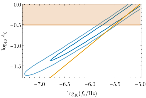
Already at this stage, the degeneracy allows the parameter space to extend to much higher frequencies than the nanohertz ballpark. This indicates that the new data analyses by the PTA collaborations prefer smaller-mass PBHs than expected so far.
III Implications for primordial black holes
In this section, we show that sub-solar mass PBHs are favored by the new data. To this end, we summarize the formulas for PBHs. The formulas are basically the same as those in Ref. [99].111 The abundance of PBHs is subject to a huge uncertainty depending on the calculation scheme. For example, our prescription here is based on Carr’s formula (a.k.a. the Press-Schechter formalism) [107], but the result changes significantly when one adopts the peaks theory, within which there are varieties of methods with varying results [108, 109, 110, 111, 112, 113, 114, 115, 116, 117]. PBHs are formed shortly after an extremely enhanced curvature perturbation enters the Hubble horizon [118, 119, 107]. Therefore, the mass of PBHs is related to the wavenumber of the perturbations that produce PBHs
| (12) |
where is the ratio between the PBH mass and the horizon mass, for which we take as a fiducial value [107], and is the temperature at the PBH production.
The PBH abundance per log bin in is given by [120] 222The tilde on is introduced to distinguish it with its integrated quantity .
| (13) |
The production rate is given by [107]
| (14) |
where is the threshold value of the overdensity for PBH production. As a fiducial value, we take [121, 122, 123, 124, 99]. The is the coarse-grained density contrast, given by
| (15) |
Here, is a window function, which we take , and is the transfer function of the density perturbations during an RD era:
| (16) |
The total abundance of the PBHs can be expressed as
| (17) |

In the case of the monochromatic power spectrum, can be integrated analytically
| (18) |
where . Combining these equations and the parameter degeneracy relation Eq. (11), we can map the degeneracy relation onto the - plane:
| (19) |
where we have approximated as . The coefficient is introduced to show the sensitivity of on the overall normalization of . In Fig. 2, we set . The slope does not fit perfectly because the GW spectrum does not have a perfect scaling. This equation is not a rigorous fit but just a rough guide to the location of the contours mapped from Fig. 1 into Fig. 2.
The blue contours in Fig. 2 are the main result of this paper. This shows that the PBHs much lighter than the Sun are favored by the new PTA data analysis results. If the PBH abundance is significant, they have masses of order . More generally, the contours show the range []. It should be emphasized that this is based on the assumption of the delta function , but our conclusion would not qualitatively change even if we take into account the finite width of the realistic power spectrum.
The shaded regions in the upper part of Fig. 2 show the existing observational constraints on the abundance of PBHs. We see that there is a lower as well as an upper bound on the mass of the PBHs. In other words, the extension to the degeneracy direction is limited by the overproduction of PBHs. Again, the quantitative values of these bounds will change when we drop off the assumption of the delta function curvature spectrum, but our conclusion will be intact at least when the power spectrum has a narrow peak. See the analyses of NANOGrav [99] and EPTA/InPTA [6] for the curvature spectra with a finite width.
IV Conclusion and Discussion
In this work, we have discussed the implications of the recent PTA observations of stochastic GWs on PBHs. The large scalar perturbations can produce not only PBHs but also strong GWs through nonlinear interactions. If the detected stochastic GWs originate from scalar-induced GWs, we can obtain implications on the PBH mass distribution. We have found that, if PBHs are produced by the monochromatic curvature power spectrum, the stochastic GW signals can be explained by the large-scale tail of the induced GW spectrum.
It is interesting to note that the favored region on the - plane to explain the excess events of OGLE [126] (the yellow shaded region in Fig. 2) [125], has a small overlap with the blue contours in Fig. 2.333 The relation between the 12.5-year NANOGrav data and the OGLE events has been studied in the context of PBHs produced during an era with a general in Ref. [35]. It is remarkable that the OGLE microlensing events and the SGWB signals from the PTA data can be simultaneously explained by PBHs of mass . Remember that our analyses are based on the delta-function curvature spectrum for simplicity. It is interesting if the overlap becomes larger when we consider a more realistic curvature perturbation spectrum. We leave this possibility for future work.
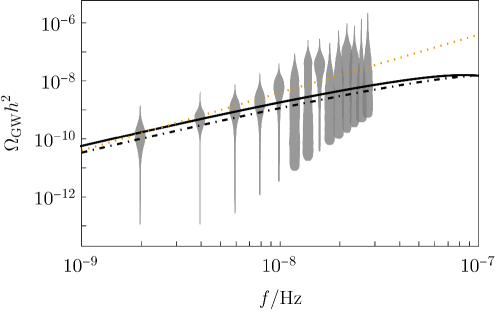
Examples of the scalar-induced GW spectrum are shown in Fig. 3 in comparison with the 14 lowest-frequency bins (see Appendix C of Ref. [2]) of the NANOGrav 15-year data [99]. The black solid line corresponds to and , which is inside the 68% credible region (dark blue contour) in Fig. 2. The black dot-dashed line corresponds to and , which is inside the 95% credible region (light blue contour) and the yellow shaded region to explain the OGLE events.
In our previous work [34], we discussed that the PBH interpretation of the common-spectral processes in the NANOGrav data can be tested by future observations of GWs at a different frequency range originating from the merger events of the binary PBHs. This also constitutes the SGWB because of the superposition of many binary mergers in the Universe. In this letter, we have emphasized that the preferred mass range of PBHs associated with the induced GWs that explain the new PTA data is shifted to a smaller mass range. It is then natural to ask about the corresponding change of the observational prospects to test the PBH scenario.
To calculate the merger-based GW spectrum, we have adopted the methods concisely summarized in Appendices of Ref. [164], essentially based on the merger rate calculations in Refs. [65, 69] and the source-frame spectrum emitted at a single merger event studied in Refs. [165, 166]. For simplicity, we take the representing mass corresponding to and neglect the mass distribution of PBHs in the calculation of the merger-based GW spectrum. The extension of the spectrum to the far IR may break down at some frequency as discussed in Appendix B of Ref. [167].
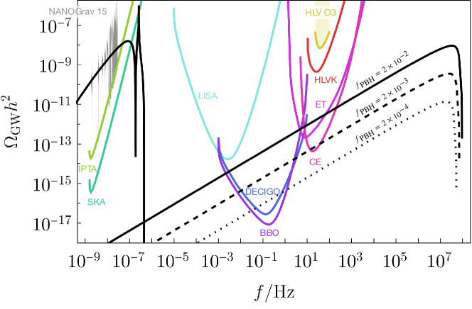
The comparison of the merger-based GWs (shown by black lines) and the sensitivity curves of future GW detectors is shown in Fig. 4. Compared to Fig. 5 in Ref. [34], the peaks of the merger-based GWs are shifted to the high-frequency side. This is because the corresponding binary PBH masses have become lighter in view of the new PTA data. Unfortunately, the observational prospects by the future GW detectors become worse due to this frequency shift. Nevertheless, Fig. 4 shows that the SGWB originating from PBH binary mergers can be tested by future GW observations.444 We adopted different sensitivity curves from those adopted in the previous work [34]. See the caption of Fig. 4. To achieve this goal, foreground subtraction is essential [145, 168].555 We thank Marek Lewicki for his comment on this point. An alternative route is the development of MHz–GHz GW detectors. See, e.g., Refs. [169, 170] and references therein.
Our results are consistent with those in Ref. [99] because we basically use the same equations and take similar values of the parameters as in the reference. However, as mentioned in Ref. [56], our results and those in Ref. [99] on the PBH abundance are different from those in Ref. [56], in which they show that PBHs are overproduced if we do not take into account the non-Gaussianity that decreases the PBH abundance with the amplitude of the induced GWs fixed.666 The possibility of the PBH overproduction was also discussed with the IPTA Data Release 2 and the NANOGrav 12.5-year datasets in Ref. [39]. Although we do not take into account the non-Gaussianity that decreases the PBH abundance, we have still found that PBHs are not overproduced. The main discrepancy comes from the difference in the window function and/or the threshold value, , as mentioned in Ref. [56]. Our results show that whether the recent detection of the stochastic GWs is associated with PBHs or not significantly depends on the uncertainties on the choice of window function and/or .
One of the reasons why we focus on the delta function curvature spectrum in this paper even though it is unrealistic is the scaling suggested by Fig. 1 (b) of the NANOGrav paper [2] as discussed above. It is tempting to argue that naively combining the new data (DR2new) analysis and the full data (DR2full) analysis in Fig. 1 of EPTA/InPTA paper [4], would be obtained. However, one should be careful about the combination of data sets in mild tension. It will be interesting to discuss how well the narrow peak PBH scenarios can also explain the data of other PTA collaborations. We will leave such comprehensive analyses for future work.
Acknowledgements.
K.I. and T.T. thank Satoshi Shirai for stimulating discussions. K.I. was supported by the Kavli Institute for Cosmological Physics at the University of Chicago through an endowment from the Kavli Foundation and its founder Fred Kavli. The work of T.T. was supported by IBS under the project code, IBS-R018-D1. The work of K.K. was in part supported by MEXT KAKENHI Grant Number JP22H05270.References
- Hellings and Downs [1983] R. W. Hellings and G. S. Downs, Astrophys. J. 265, L39 (1983).
- Agazie et al. [2023a] G. Agazie et al. (NANOGrav), Astrophys. J. Lett. 951 (2023a), 10.3847/2041-8213/acdac6, arXiv:2306.16213 [astro-ph.HE] .
- Agazie et al. [2023b] G. Agazie et al. (NANOGrav), Astrophys. J. Lett. 951 (2023b), 10.3847/2041-8213/acda9a, arXiv:2306.16217 [astro-ph.HE] .
- Antoniadis et al. [2023a] J. Antoniadis et al., (2023a), arXiv:2306.16214 [astro-ph.HE] .
- Antoniadis et al. [2023b] J. Antoniadis et al., (2023b), 10.1051/0004-6361/202346841, arXiv:2306.16224 [astro-ph.HE] .
- Antoniadis et al. [2023c] J. Antoniadis et al., (2023c), arXiv:2306.16227 [astro-ph.CO] .
- Reardon et al. [2023a] D. J. Reardon et al., Astrophys. J. Lett. 951 (2023a), 10.3847/2041-8213/acdd02, arXiv:2306.16215 [astro-ph.HE] .
- Zic et al. [2023] A. Zic et al., (2023), arXiv:2306.16230 [astro-ph.HE] .
- Reardon et al. [2023b] D. J. Reardon et al., (2023b), 10.3847/2041-8213/acdd03, arXiv:2306.16229 [astro-ph.HE] .
- Xu et al. [2023] H. Xu et al., (2023), 10.1088/1674-4527/acdfa5, arXiv:2306.16216 [astro-ph.HE] .
- Agazie et al. [2023c] G. Agazie et al. (NANOGrav), (2023c), arXiv:2306.16221 [astro-ph.HE] .
- Agazie et al. [2023d] G. Agazie et al. (NANOGrav), (2023d), arXiv:2306.16222 [astro-ph.HE] .
- Antoniadis et al. [2023d] J. Antoniadis et al., (2023d), arXiv:2306.16226 [astro-ph.HE] .
- Arzoumanian et al. [2020] Z. Arzoumanian et al. (NANOGrav), Astrophys. J. Lett. 905, L34 (2020), arXiv:2009.04496 [astro-ph.HE] .
- Antoniadis et al. [2022] J. Antoniadis et al., Mon. Not. Roy. Astron. Soc. 510, 4873 (2022), arXiv:2201.03980 [astro-ph.HE] .
- Ellis and Lewicki [2021] J. Ellis and M. Lewicki, Phys. Rev. Lett. 126, 041304 (2021), arXiv:2009.06555 [astro-ph.CO] .
- Datta et al. [2021] S. Datta, A. Ghosal, and R. Samanta, JCAP 08, 021 (2021), arXiv:2012.14981 [hep-ph] .
- Samanta and Datta [2021] R. Samanta and S. Datta, JHEP 05, 211 (2021), arXiv:2009.13452 [hep-ph] .
- Buchmuller et al. [2020] W. Buchmuller, V. Domcke, and K. Schmitz, Phys. Lett. B 811, 135914 (2020), arXiv:2009.10649 [astro-ph.CO] .
- Blanco-Pillado et al. [2021] J. J. Blanco-Pillado, K. D. Olum, and J. M. Wachter, Phys. Rev. D 103, 103512 (2021), arXiv:2102.08194 [astro-ph.CO] .
- Ferreira et al. [2023] R. Z. Ferreira, A. Notari, O. Pujolas, and F. Rompineve, JCAP 02, 001 (2023), arXiv:2204.04228 [astro-ph.CO] .
- Arzoumanian et al. [2021] Z. Arzoumanian et al. (NANOGrav), Phys. Rev. Lett. 127, 251302 (2021), arXiv:2104.13930 [astro-ph.CO] .
- Xue et al. [2021] X. Xue et al., Phys. Rev. Lett. 127, 251303 (2021), arXiv:2110.03096 [astro-ph.CO] .
- Nakai et al. [2021] Y. Nakai, M. Suzuki, F. Takahashi, and M. Yamada, Phys. Lett. B 816, 136238 (2021), arXiv:2009.09754 [astro-ph.CO] .
- Di Bari et al. [2021] P. Di Bari, D. Marfatia, and Y.-L. Zhou, JHEP 10, 193 (2021), arXiv:2106.00025 [hep-ph] .
- Sakharov et al. [2021] A. S. Sakharov, Y. N. Eroshenko, and S. G. Rubin, Phys. Rev. D 104, 043005 (2021), arXiv:2104.08750 [hep-ph] .
- Li et al. [2021a] S.-L. Li, L. Shao, P. Wu, and H. Yu, Phys. Rev. D 104, 043510 (2021a), arXiv:2101.08012 [astro-ph.CO] .
- Ashoorioon et al. [2022] A. Ashoorioon, K. Rezazadeh, and A. Rostami, Phys. Lett. B 835, 137542 (2022), arXiv:2202.01131 [astro-ph.CO] .
- Benetti et al. [2022] M. Benetti, L. L. Graef, and S. Vagnozzi, Phys. Rev. D 105, 043520 (2022), arXiv:2111.04758 [astro-ph.CO] .
- Barir et al. [2022] J. Barir, M. Geller, C. Sun, and T. Volansky, (2022), arXiv:2203.00693 [hep-ph] .
- Hindmarsh and Kume [2023] M. Hindmarsh and J. Kume, JCAP 04, 045 (2023), arXiv:2210.06178 [astro-ph.CO] .
- Vaskonen and Veermäe [2021] V. Vaskonen and H. Veermäe, Phys. Rev. Lett. 126, 051303 (2021), arXiv:2009.07832 [astro-ph.CO] .
- De Luca et al. [2021] V. De Luca, G. Franciolini, and A. Riotto, Phys. Rev. Lett. 126, 041303 (2021), arXiv:2009.08268 [astro-ph.CO] .
- Kohri and Terada [2021] K. Kohri and T. Terada, Phys. Lett. B 813, 136040 (2021), arXiv:2009.11853 [astro-ph.CO] .
- Domènech and Pi [2022] G. Domènech and S. Pi, Sci. China Phys. Mech. Astron. 65, 230411 (2022), arXiv:2010.03976 [astro-ph.CO] .
- Papanikolaou et al. [2021] T. Papanikolaou, V. Vennin, and D. Langlois, JCAP 03, 053 (2021), arXiv:2010.11573 [astro-ph.CO] .
- Inomata et al. [2021] K. Inomata, M. Kawasaki, K. Mukaida, and T. T. Yanagida, Phys. Rev. Lett. 126, 131301 (2021), arXiv:2011.01270 [astro-ph.CO] .
- Kawasaki and Nakatsuka [2021] M. Kawasaki and H. Nakatsuka, JCAP 05, 023 (2021), arXiv:2101.11244 [astro-ph.CO] .
- Dandoy et al. [2023] V. Dandoy, V. Domcke, and F. Rompineve, (2023), arXiv:2302.07901 [astro-ph.CO] .
- Vagnozzi [2021] S. Vagnozzi, Mon. Not. Roy. Astron. Soc. 502, L11 (2021), arXiv:2009.13432 [astro-ph.CO] .
- Li et al. [2021b] H.-H. Li, G. Ye, and Y.-S. Piao, Phys. Lett. B 816, 136211 (2021b), arXiv:2009.14663 [astro-ph.CO] .
- Bhattacharya et al. [2021] S. Bhattacharya, S. Mohanty, and P. Parashari, Phys. Rev. D 103, 063532 (2021), arXiv:2010.05071 [astro-ph.CO] .
- Kuroyanagi et al. [2021] S. Kuroyanagi, T. Takahashi, and S. Yokoyama, JCAP 01, 071 (2021), arXiv:2011.03323 [astro-ph.CO] .
- Madge et al. [2023] E. Madge, E. Morgante, C. P. Ibáñez, N. Ramberg, and S. Schenk, (2023), arXiv:2306.14856 [hep-ph] .
- Ellis et al. [2023] J. Ellis, M. Lewicki, C. Lin, and V. Vaskonen, (2023), arXiv:2306.17147 [astro-ph.CO] .
- Wang et al. [2023] Z. Wang, L. Lei, H. Jiao, L. Feng, and Y.-Z. Fan, (2023), arXiv:2306.17150 [astro-ph.HE] .
- King et al. [2023] S. F. King, D. Marfatia, and M. H. Rahat, (2023), arXiv:2306.05389v2 [hep-ph] .
- Guo et al. [2023] S.-Y. Guo, M. Khlopov, X. Liu, L. Wu, Y. Wu, and B. Zhu, (2023), arXiv:2306.17022 [hep-ph] .
- Kitajima et al. [2023] N. Kitajima, J. Lee, K. Murai, F. Takahashi, and W. Yin, (2023), arXiv:2306.17146 [hep-ph] .
- Bai et al. [2023] Y. Bai, T.-K. Chen, and M. Korwar, (2023), arXiv:2306.17160 [hep-ph] .
- Zu et al. [2023] L. Zu, C. Zhang, Y.-Y. Li, Y.-C. Gu, Y.-L. S. Tsai, and Y.-Z. Fan, (2023), arXiv:2306.16769 [astro-ph.HE] .
- Han et al. [2023] C. Han, K.-P. Xie, J. M. Yang, and M. Zhang, (2023), arXiv:2306.16966 [hep-ph] .
- Megias et al. [2023] E. Megias, G. Nardini, and M. Quiros, (2023), arXiv:2306.17071 [hep-ph] .
- Fujikura et al. [2023] K. Fujikura, S. Girmohanta, Y. Nakai, and M. Suzuki, (2023), arXiv:2306.17086 [hep-ph] .
- Vagnozzi [2023] S. Vagnozzi, (2023), arXiv:2306.16912 [astro-ph.CO] .
- Franciolini et al. [2023a] G. Franciolini, A. Iovino, Junior., V. Vaskonen, and H. Veermae, (2023a), arXiv:2306.17149 [astro-ph.CO] .
- Kitajima and Takahashi [2023] N. Kitajima and T. Takahashi, (2023), arXiv:2306.16896 [astro-ph.CO] .
- Li et al. [2023] Y. Li, C. Zhang, Z. Wang, M. Cui, Y.-L. S. Tsai, Q. Yuan, and Y.-Z. Fan, (2023), arXiv:2306.17124 [astro-ph.HE] .
- Yang et al. [2023] J. Yang, N. Xie, and F. P. Huang, (2023), arXiv:2306.17113 [hep-ph] .
- Franciolini et al. [2023b] G. Franciolini, D. Racco, and F. Rompineve, (2023b), arXiv:2306.17136 [astro-ph.CO] .
- Lambiase et al. [2023] G. Lambiase, L. Mastrototaro, and L. Visinelli, (2023), arXiv:2306.16977 [astro-ph.HE] .
- Ghoshal and Strumia [2023] A. Ghoshal and A. Strumia, (2023), arXiv:2306.17158 [astro-ph.CO] .
- Bird et al. [2016] S. Bird, I. Cholis, J. B. Muñoz, Y. Ali-Haïmoud, M. Kamionkowski, E. D. Kovetz, A. Raccanelli, and A. G. Riess, Phys. Rev. Lett. 116, 201301 (2016), arXiv:1603.00464 [astro-ph.CO] .
- Clesse and García-Bellido [2017] S. Clesse and J. García-Bellido, Phys. Dark Univ. 15, 142 (2017), arXiv:1603.05234 [astro-ph.CO] .
- Sasaki et al. [2016] M. Sasaki, T. Suyama, T. Tanaka, and S. Yokoyama, Phys. Rev. Lett. 117, 061101 (2016), arXiv:1603.08338 [astro-ph.CO] .
- Kashlinsky [2016] A. Kashlinsky, Astrophys. J. Lett. 823, L25 (2016), arXiv:1605.04023 [astro-ph.CO] .
- Kashlinsky et al. [2018] A. Kashlinsky, R. G. Arendt, F. Atrio-Barandela, N. Cappelluti, A. Ferrara, and G. Hasinger, Rev. Mod. Phys. 90, 025006 (2018), arXiv:1802.07774 [astro-ph.CO] .
- García-Bellido et al. [2021] J. García-Bellido, J. F. Nuño Siles, and E. Ruiz Morales, Phys. Dark Univ. 31, 100791 (2021), arXiv:2010.13811 [astro-ph.CO] .
- Sasaki et al. [2018] M. Sasaki, T. Suyama, T. Tanaka, and S. Yokoyama, Class. Quant. Grav. 35, 063001 (2018), arXiv:1801.05235 [astro-ph.CO] .
- Carr et al. [2021] B. Carr, K. Kohri, Y. Sendouda, and J. Yokoyama, Rept. Prog. Phys. 84, 116902 (2021), arXiv:2002.12778 [astro-ph.CO] .
- Green and Kavanagh [2021] A. M. Green and B. J. Kavanagh, J. Phys. G 48, 043001 (2021), arXiv:2007.10722 [astro-ph.CO] .
- Escrivà et al. [2022] A. Escrivà, F. Kuhnel, and Y. Tada, (2022), arXiv:2211.05767 [astro-ph.CO] .
- Ananda et al. [2007] K. N. Ananda, C. Clarkson, and D. Wands, Phys. Rev. D75, 123518 (2007), arXiv:gr-qc/0612013 [gr-qc] .
- Baumann et al. [2007] D. Baumann, P. J. Steinhardt, K. Takahashi, and K. Ichiki, Phys. Rev. D76, 084019 (2007), arXiv:hep-th/0703290 [hep-th] .
- Saito and Yokoyama [2009] R. Saito and J. Yokoyama, Phys. Rev. Lett. 102, 161101 (2009), [Erratum: Phys. Rev. Lett.107,069901(2011)], arXiv:0812.4339 [astro-ph] .
- Saito and Yokoyama [2010] R. Saito and J. Yokoyama, Prog. Theor. Phys. 123, 867 (2010), [Erratum: Prog. Theor. Phys.126,351(2011)], arXiv:0912.5317 [astro-ph.CO] .
- Inomata et al. [2017] K. Inomata, M. Kawasaki, K. Mukaida, Y. Tada, and T. T. Yanagida, Phys. Rev. D95, 123510 (2017), arXiv:1611.06130 [astro-ph.CO] .
- Ando et al. [2018a] K. Ando, K. Inomata, M. Kawasaki, K. Mukaida, and T. T. Yanagida, Phys. Rev. D97, 123512 (2018a), arXiv:1711.08956 [astro-ph.CO] .
- Espinosa et al. [2018] J. R. Espinosa, D. Racco, and A. Riotto, JCAP 1809, 012 (2018), arXiv:1804.07732 [hep-ph] .
- Kohri and Terada [2018a] K. Kohri and T. Terada, Phys. Rev. D97, 123532 (2018a), arXiv:1804.08577 [gr-qc] .
- Cai et al. [2018] R.-g. Cai, S. Pi, and M. Sasaki, (2018), arXiv:1810.11000 [astro-ph.CO] .
- Bartolo et al. [2018a] N. Bartolo, V. De Luca, G. Franciolini, M. Peloso, and A. Riotto, (2018a), arXiv:1810.12218 [astro-ph.CO] .
- Bartolo et al. [2018b] N. Bartolo, V. De Luca, G. Franciolini, M. Peloso, D. Racco, and A. Riotto, (2018b), arXiv:1810.12224 [astro-ph.CO] .
- Unal [2018] C. Unal, (2018), arXiv:1811.09151 [astro-ph.CO] .
- Byrnes et al. [2018] C. T. Byrnes, P. S. Cole, and S. P. Patil, (2018), arXiv:1811.11158 [astro-ph.CO] .
- Inomata and Nakama [2019] K. Inomata and T. Nakama, Phys. Rev. D99, 043511 (2019), arXiv:1812.00674 [astro-ph.CO] .
- Clesse et al. [2018] S. Clesse, J. García-Bellido, and S. Orani, (2018), arXiv:1812.11011 [astro-ph.CO] .
- Cai et al. [2019a] R.-G. Cai, S. Pi, S.-J. Wang, and X.-Y. Yang, JCAP 05, 013 (2019a), arXiv:1901.10152 [astro-ph.CO] .
- Cai et al. [2019b] Y.-F. Cai, C. Chen, X. Tong, D.-G. Wang, and S.-F. Yan, Phys. Rev. D 100, 043518 (2019b), arXiv:1902.08187 [astro-ph.CO] .
- Chen et al. [2020] Z.-C. Chen, C. Yuan, and Q.-G. Huang, Phys. Rev. Lett. 124, 251101 (2020), arXiv:1910.12239 [astro-ph.CO] .
- Domènech [2021] G. Domènech, Universe 7, 398 (2021), arXiv:2109.01398 [gr-qc] .
- Yuan and Huang [2021] C. Yuan and Q.-G. Huang, (2021), arXiv:2103.04739 [astro-ph.GA] .
- Orlofsky et al. [2017] N. Orlofsky, A. Pierce, and J. D. Wells, Phys. Rev. D95, 063518 (2017), arXiv:1612.05279 [astro-ph.CO] .
- Nakama et al. [2017] T. Nakama, J. Silk, and M. Kamionkowski, Phys. Rev. D95, 043511 (2017), arXiv:1612.06264 [astro-ph.CO] .
- Garcia-Bellido et al. [2017] J. Garcia-Bellido, M. Peloso, and C. Unal, JCAP 1709, 013 (2017), arXiv:1707.02441 [astro-ph.CO] .
- Di and Gong [2018] H. Di and Y. Gong, JCAP 07, 007 (2018), arXiv:1707.09578 [astro-ph.CO] .
- Cheng et al. [2018] S.-L. Cheng, W. Lee, and K.-W. Ng, JCAP 07, 001 (2018), arXiv:1801.09050 [astro-ph.CO] .
- Kohri and Terada [2018b] K. Kohri and T. Terada, Class. Quant. Grav. 35, 235017 (2018b), arXiv:1802.06785 [astro-ph.CO] .
- Afzal et al. [2023] A. Afzal et al. (NANOGrav), Astrophys. J. Lett. 951 (2023), 10.3847/2041-8213/acdc91, arXiv:2306.16219 [astro-ph.HE] .
- Arzoumanian et al. [2018] Z. Arzoumanian et al. (NANOGRAV), Astrophys. J. 859, 47 (2018), arXiv:1801.02617 [astro-ph.HE] .
- Cai et al. [2020] R.-G. Cai, S. Pi, and M. Sasaki, Phys. Rev. D 102, 083528 (2020), arXiv:1909.13728 [astro-ph.CO] .
- Yuan et al. [2020] C. Yuan, Z.-C. Chen, and Q.-G. Huang, Phys. Rev. D 101, 043019 (2020), arXiv:1910.09099 [astro-ph.CO] .
- Domènech et al. [2020] G. Domènech, S. Pi, and M. Sasaki, JCAP 08, 017 (2020), arXiv:2005.12314 [gr-qc] .
- Pi and Sasaki [2020] S. Pi and M. Sasaki, JCAP 09, 037 (2020), arXiv:2005.12306 [gr-qc] .
- Saikawa and Shirai [2018] K. Saikawa and S. Shirai, JCAP 05, 035 (2018), arXiv:1803.01038 [hep-ph] .
- Clarke et al. [2020] T. J. Clarke, E. J. Copeland, and A. Moss, JCAP 10, 002 (2020), arXiv:2004.11396 [astro-ph.CO] .
- Carr [1975] B. J. Carr, Astrophys. J. 201, 1 (1975).
- Bardeen et al. [1986] J. M. Bardeen, J. R. Bond, N. Kaiser, and A. S. Szalay, Astrophys. J. 304, 15 (1986).
- Yoo et al. [2018] C.-M. Yoo, T. Harada, J. Garriga, and K. Kohri, (2018), arXiv:1805.03946 [astro-ph.CO] .
- Germani and Musco [2019] C. Germani and I. Musco, Phys. Rev. Lett. 122, 141302 (2019), arXiv:1805.04087 [astro-ph.CO] .
- Young [2019] S. Young, Int. J. Mod. Phys. D 29, 2030002 (2019), arXiv:1905.01230 [astro-ph.CO] .
- Suyama and Yokoyama [2020] T. Suyama and S. Yokoyama, PTEP 2020, 023E03 (2020), arXiv:1912.04687 [astro-ph.CO] .
- Germani and Sheth [2020] C. Germani and R. K. Sheth, Phys. Rev. D 101, 063520 (2020), arXiv:1912.07072 [astro-ph.CO] .
- Young and Musso [2020] S. Young and M. Musso, JCAP 11, 022 (2020), arXiv:2001.06469 [astro-ph.CO] .
- Yoo et al. [2021] C.-M. Yoo, T. Harada, S. Hirano, and K. Kohri, PTEP 2021, 013E02 (2021), arXiv:2008.02425 [astro-ph.CO] .
- Musco et al. [2021] I. Musco, V. De Luca, G. Franciolini, and A. Riotto, Phys. Rev. D 103, 063538 (2021), arXiv:2011.03014 [astro-ph.CO] .
- Young [2022] S. Young, JCAP 05, 037 (2022), arXiv:2201.13345 [astro-ph.CO] .
- Hawking [1971] S. Hawking, Mon. Not. Roy. Astron. Soc. 152, 75 (1971).
- Carr and Hawking [1974] B. J. Carr and S. W. Hawking, Mon. Not. Roy. Astron. Soc. 168, 399 (1974).
- Ando et al. [2018b] K. Ando, K. Inomata, and M. Kawasaki, Phys. Rev. D97, 103528 (2018b), arXiv:1802.06393 [astro-ph.CO] .
- Harada et al. [2013] T. Harada, C.-M. Yoo, and K. Kohri, Phys. Rev. D88, 084051 (2013), [Erratum: Phys. Rev.D89,no.2,029903(2014)], arXiv:1309.4201 [astro-ph.CO] .
- Musco et al. [2005] I. Musco, J. C. Miller, and L. Rezzolla, Class. Quant. Grav. 22, 1405 (2005), arXiv:gr-qc/0412063 [gr-qc] .
- Polnarev and Musco [2007] A. G. Polnarev and I. Musco, Class. Quant. Grav. 24, 1405 (2007), arXiv:gr-qc/0605122 .
- Musco and Miller [2013] I. Musco and J. C. Miller, Class. Quant. Grav. 30, 145009 (2013), arXiv:1201.2379 [gr-qc] .
- Niikura et al. [2019] H. Niikura, M. Takada, S. Yokoyama, T. Sumi, and S. Masaki, Phys. Rev. D 99, 083503 (2019), arXiv:1901.07120 [astro-ph.CO] .
- Mróz et al. [2017] P. Mróz, A. Udalski, J. Skowron, R. Poleski, S. Kozłowski, M. K. Szymański, I. Soszyński, Ł. Wyrzykowski, P. Pietrukowicz, K. Ulaczyk, D. Skowron, and M. Pawlak, Nature (London) 548, 183 (2017), arXiv:1707.07634 [astro-ph.EP] .
- Niikura et al. [2017] H. Niikura, M. Takada, N. Yasuda, R. H. Lupton, T. Sumi, S. More, A. More, M. Oguri, and M. Chiba, (2017), arXiv:1701.02151 [astro-ph.CO] .
- Tisserand et al. [2007] P. Tisserand et al. (EROS-2), Astron. Astrophys. 469, 387 (2007), arXiv:astro-ph/0607207 .
- Allsman et al. [2001] R. A. Allsman et al. (Macho), Astrophys. J. Lett. 550, L169 (2001), arXiv:astro-ph/0011506 .
- Oguri et al. [2018] M. Oguri, J. M. Diego, N. Kaiser, P. L. Kelly, and T. Broadhurst, Phys. Rev. D 97, 023518 (2018), arXiv:1710.00148 [astro-ph.CO] .
- Wang et al. [2016] S. Wang, Y.-F. Wang, Q.-G. Huang, and T. G. F. Li, (2016), arXiv:1610.08725 [astro-ph.CO] .
- Chen and Huang [2020] Z.-C. Chen and Q.-G. Huang, JCAP 08, 039 (2020), arXiv:1904.02396 [astro-ph.CO] .
- Abbott et al. [2019] B. Abbott et al. (LIGO Scientific, Virgo), Phys. Rev. D 100, 061101 (2019), arXiv:1903.02886 [gr-qc] .
- Abbott et al. [2021] R. Abbott et al. (KAGRA, Virgo, LIGO Scientific), Phys. Rev. D 104, 022004 (2021), arXiv:2101.12130 [gr-qc] .
- Hobbs et al. [2010] G. Hobbs et al., Class. Quant. Grav. 27, 084013 (2010), arXiv:0911.5206 [astro-ph.SR] .
- Manchester [2013] R. N. Manchester, Class. Quant. Grav. 30, 224010 (2013), arXiv:1309.7392 [astro-ph.IM] .
- Carilli and Rawlings [2004] C. L. Carilli and S. Rawlings, New Astron. Rev. 48, 979 (2004), arXiv:astro-ph/0409274 .
- Janssen et al. [2015] G. Janssen et al., Proceedings, Advancing Astrophysics with the Square Kilometre Array (AASKA14): Giardini Naxos, Italy, June 9-13, 2014, PoS AASKA14, 037 (2015), arXiv:1501.00127 [astro-ph.IM] .
- Weltman et al. [2020] A. Weltman et al., Publ. Astron. Soc. Austral. 37, e002 (2020), arXiv:1810.02680 [astro-ph.CO] .
- Amaro-Seoane et al. [2017] P. Amaro-Seoane et al. (LISA), (2017), arXiv:1702.00786 [astro-ph.IM] .
- Baker et al. [2019] J. Baker et al., (2019), arXiv:1907.06482 [astro-ph.IM] .
- Seto et al. [2001] N. Seto, S. Kawamura, and T. Nakamura, Phys. Rev. Lett. 87, 221103 (2001), arXiv:astro-ph/0108011 [astro-ph] .
- Yagi and Seto [2011] K. Yagi and N. Seto, Phys. Rev. D83, 044011 (2011), [Erratum: Phys. Rev.D95,no.10,109901(2017)], arXiv:1101.3940 [astro-ph.CO] .
- Isoyama et al. [2018] S. Isoyama, H. Nakano, and T. Nakamura, PTEP 2018, 073E01 (2018), arXiv:1802.06977 [gr-qc] .
- Kawamura et al. [2021] S. Kawamura et al., PTEP 2021, 05A105 (2021), arXiv:2006.13545 [gr-qc] .
- Crowder and Cornish [2005] J. Crowder and N. J. Cornish, Phys. Rev. D 72, 083005 (2005), arXiv:gr-qc/0506015 .
- Corbin and Cornish [2006] V. Corbin and N. J. Cornish, Class. Quant. Grav. 23, 2435 (2006), arXiv:gr-qc/0512039 .
- Harry et al. [2006] G. M. Harry, P. Fritschel, D. A. Shaddock, W. Folkner, and E. S. Phinney, Class. Quant. Grav. 23, 4887 (2006), [Erratum: Class. Quant. Grav.23,7361(2006)].
- Punturo et al. [2010] M. Punturo et al., Proceedings, 14th Workshop on Gravitational wave data analysis (GWDAW-14): Rome, Italy, January 26-29, 2010, Class. Quant. Grav. 27, 194002 (2010).
- Hild et al. [2011] S. Hild et al., Class. Quant. Grav. 28, 094013 (2011), arXiv:1012.0908 [gr-qc] .
- Sathyaprakash et al. [2012] B. Sathyaprakash et al., Class. Quant. Grav. 29, 124013 (2012), [Erratum: Class.Quant.Grav. 30, 079501 (2013)], arXiv:1206.0331 [gr-qc] .
- Maggiore et al. [2020] M. Maggiore et al., JCAP 03, 050 (2020), arXiv:1912.02622 [astro-ph.CO] .
- Abbott et al. [2017] B. P. Abbott et al. (LIGO Scientific), Class. Quant. Grav. 34, 044001 (2017), arXiv:1607.08697 [astro-ph.IM] .
- Reitze et al. [2019] D. Reitze et al., Bull. Am. Astron. Soc. 51, 035 (2019), arXiv:1907.04833 [astro-ph.IM] .
- Harry [2010] G. M. Harry (LIGO Scientific), Class. Quant. Grav. 27, 084006 (2010).
- Aasi et al. [2015] J. Aasi et al. (LIGO Scientific), Class. Quant. Grav. 32, 074001 (2015), arXiv:1411.4547 [gr-qc] .
- Acernese et al. [2015] F. Acernese et al. (VIRGO), Class. Quant. Grav. 32, 024001 (2015), arXiv:1408.3978 [gr-qc] .
- Somiya [2012] K. Somiya (KAGRA), Class. Quant. Grav. 29, 124007 (2012), arXiv:1111.7185 [gr-qc] .
- Aso et al. [2013] Y. Aso, Y. Michimura, K. Somiya, M. Ando, O. Miyakawa, T. Sekiguchi, D. Tatsumi, and H. Yamamoto (KAGRA), Phys. Rev. D 88, 043007 (2013), arXiv:1306.6747 [gr-qc] .
- Akutsu et al. [2019a] T. Akutsu et al. (KAGRA), Nature Astron. 3, 35 (2019a), arXiv:1811.08079 [gr-qc] .
- Akutsu et al. [2019b] T. Akutsu et al. (KAGRA), Class. Quant. Grav. 36, 165008 (2019b), arXiv:1901.03569 [astro-ph.IM] .
- Michimura et al. [2019] Y. Michimura et al., in 15th Marcel Grossmann Meeting on Recent Developments in Theoretical and Experimental General Relativity, Astrophysics, and Relativistic Field Theories (2019) arXiv:1906.02866 [gr-qc] .
- Schmitz [2021] K. Schmitz, JHEP 01, 097 (2021), arXiv:2002.04615 [hep-ph] .
- Wang et al. [2019] S. Wang, T. Terada, and K. Kohri, Phys. Rev. D 99, 103531 (2019), [Erratum: Phys.Rev.D 101, 069901 (2020)], arXiv:1903.05924 [astro-ph.CO] .
- Ajith et al. [2008] P. Ajith et al., Phys. Rev. D 77, 104017 (2008), [Erratum: Phys.Rev.D 79, 129901 (2009)], arXiv:0710.2335 [gr-qc] .
- Ajith et al. [2011] P. Ajith et al., Phys. Rev. Lett. 106, 241101 (2011), arXiv:0909.2867 [gr-qc] .
- Inomata et al. [2020] K. Inomata, M. Kawasaki, K. Mukaida, T. Terada, and T. T. Yanagida, Phys. Rev. D 101, 123533 (2020), arXiv:2003.10455 [astro-ph.CO] .
- Cutler and Harms [2006] C. Cutler and J. Harms, Phys. Rev. D 73, 042001 (2006), arXiv:gr-qc/0511092 .
- Domcke and Garcia-Cely [2021] V. Domcke and C. Garcia-Cely, Phys. Rev. Lett. 126, 021104 (2021), arXiv:2006.01161 [astro-ph.CO] .
- Ito et al. [2023] A. Ito, K. Kohri, and K. Nakayama, (2023), arXiv:2305.13984 [gr-qc] .