Abstract

Effectively compressing and optimizing tensor networks requires reliable methods for fixing the latent degrees of freedom of the tensors, known as the gauge. Here we introduce a new algorithm for gauging tensor networks using belief propagation, a method that was originally formulated for performing statistical inference on graphical models and has recently found applications in tensor network algorithms. We show that this method is closely related to known tensor network gauging methods. It has the practical advantage, however, that existing belief propagation implementations can be repurposed for tensor network gauging, and that belief propagation is a very simple algorithm based on just tensor contractions so it can be easier to implement, optimize, and generalize. We present numerical evidence and scaling arguments that this algorithm is faster than existing gauging algorithms, demonstrating its usage on structured, unstructured, and infinite tensor networks. Additionally, we apply this method to improve the accuracy of the widely used simple update gate evolution algorithm.

 

 

1 Introduction

Tensor networks are low-rank approximations of high-order, potentially infinite-order, tensors as products of smaller tensors [1, 6, 7, 8, 9, 10, 11, 12, 13, 2, 3, 4, 5]. Tensor network algorithms have proven to be indispensable for studying some of the most challenging problems in condensed matter physics [14, 15, 16, 17, 18, 19, 20, 21] and quantum chemistry [22, 23, 24, 25, 26, 27]. More recently they have found new applications in an ever growing list of fields like quantum computation [28, 29, 30, 31, 32, 33, 34], machine learning [35, 36, 37, 38], numerical analysis and classical differential equation solving [39, 40, 41, 42, 43, 44, 45, 46, 47], SAT solving [48, 49], and finance [50, 51]. Algorithms for tensor networks on linear graph topologies, known as matrix product states (MPS) in the physics literature and tensor trains (TT) in the applied math literature, are extremely well developed and controlled [52, 61, 65, 66, 67, 68, 69, 70, 71, 53, 54, 41, 55, 56, 8, 57, 58, 59, 60, 62, 63, 64], even in the limit of networks with an infinite number of tensors [52, 61, 72, 73, 74, 75, 76, 77, 78, 2].

Extensions to tensor network algorithms on general tree topologies, known as tree tensor networks (TTN) in the physics literature and hierarchical Tucker (HT) decompositions in the applied math literature, are similarly well developed and controlled both in the finite [79, 84, 85, 86, 25, 87, 88, 89, 90, 80, 81, 82, 83] and infinite [91, 92, 93, 94, 95, 96, 97, 98, 99] tensor network limits. This can be attributed to a few fortuitous properties of tree tensor networks. Specifically, they are both efficient to contract exactly [100, 101] and have simple canonical forms made of locally isometric tensors that define a reduced orthogonal basis at any site in the network [66, 67, 74, 102]. This latter property has many benefits. For instance, it allows for globally optimal truncation with local operations and leads to an elegant formulation of the projector onto the tangent space of the MPS/TT [70, 103, 104, 58, 62, 105, 2, 64, 106] or TTN/HT [87, 107, 80, 81, 82] manifold. Moreover, it makes optimization and evolution algorithms for MPS/TT and TTN/HT very well behaved by allowing one to reduce the global optimization or evolution problem to an alternating series of well-conditioned and stable local updates [1, 8]. This is one of the reasons behind the huge success of the celebrated density matrix renormalization group (DMRG) algorithm of White [52, 61, 6], an extremal eigensolver for MPS/TT that has served as the basis for many subsequent algorithmic advancements.

Unfortunately, for tensor networks that involve loops, the story is not so simple. Some examples of tensor networks with loops are periodic MPS [108, 102, 109] — also known as tensor chain (TC) or tensor ring (TR) decompositions in the applied math literature [40, 110, 111] — and tensor networks with general graph connectivity known as tensor product states (TPS) or projected entangled pair states (PEPS) [112, 116, 117, 118, 119, 120, 121, 122, 123, 113, 114, 115]. Contracting tensor networks with loops is generally more costly and can only be done approximately [124], except for in special cases. Moreover, there is no single, obvious gauge that is simple to obtain for performing optimal truncations and well-behaved optimization.

Isometric gauges have been proposed for use on loopy tensor networks that reproduce many of the favorable properties of tensor network gauges on tree topologies [125, 126, 127, 128, 129, 130], but their representational power and practical usage is still under investigation and in general they can only be obtained approximately with non-local gauge transformations. Though they do not have all of the benefits of canonical forms on tree tensor networks, a number of local gauge transformations have been proposed for loopy tensor networks with various costs and benefits [119, 123, 132, 133, 134, 135, 136, 137, 138, 131]. Local gauge transformations can provide a number of uses in tensor network algorithms: enabling effective truncation of the bond dimension by identifying the most important degrees of freedom [119, 139, 122, 123, 132, 138], improving the conditioning of solvers [133, 134, 113], enhancing the effectiveness of caching environments during optimization [134, 113], and improving analysis of scaling properties of tensor networks [140]. A tensor network gauge that is commonly used for TPS/PEPS has been referred to as the ‘super-orthogonal’ [132] or ‘quasi-canonical’ [123, 134] gauge, and is a natural generalization of the ‘canonical form’ or ‘Vidal gauge’ originally defined for MPS [66, 67, 74, 75] and TTN [79, 94]. In this work, we will refer to it as the ‘Vidal gauge’ for both tree tensor networks and more general (loopy) tensor networks. The Vidal gauge for general tensor networks was originally proposed for the purpose of approximately truncating TPS/PEPS in a relatively cheap way, though potentially with a heavy approximation for networks that do not have tree-like correlations. It is the gauge implicitly used in the ‘simple update’ algorithm [119, 139, 122, 114] for updating or evolving PEPS. Finding better gauges, as well as faster and more reliable methods for gauging TNs, is of utmost importance for improving the conditioning and reliability of tensor network truncation, optimization, and evolution methods — thus expanding their use cases.

Recently, it has been noted that there is a close connection between belief propagation (BP) [141, 142, 143, 144], an algorithm originally formulated for performing statistical inference on graphical models, and tensor network contraction [145, 146, 147, 148, 149, 150, 151, 152] and gauging [153]. Belief propagation can exactly contract tensor networks on tree graphs (TTN/HT), including path graphs (MPS/TT). Additionally, it is known to work well for tensor networks on graphs that are locally tree-like, such as sparse, random graphs [149]. Here, we make the connection between belief propagation and the commonly used Vidal (or quasi-canonical/super-orthogonal) gauge that was pointed out in Ref. [153] more concrete by proposing an algorithm for using the belief propagation fixed point to gauge general tensor network states into the Vidal gauge. We refer to this new gauging method as belief propagation (BP) gauging. We compare and contrast our new gauging method to existing methods, and argue that it can be viewed as a simplified version of the gauging algorithm introduced in Refs. [132, 134]. We show examples where, for both structured and unstructured networks, our new approach is faster than currently available methods for gauging tensor network states. We also demonstrate its usage for gauging infinite tensor networks and discuss the application of this method for improving the accuracy of evolving tensor networks with ‘simple update’ [119, 114] gate evolution. Our new BP-based gauging method has the practical advantage that implementations and algorithmic advances of BP (such as the recent [151] or [154, 150]) can be repurposed for gauging tensor networks. We show an example of this in the context of approximately contracting a tensor network operator with a tensor network state. Furthermore, BP is a very simple algorithm based entirely on tensor contractions which is easy to implement efficiently for general tensor networks, something which can be exploited by our new BP-based gauging method.

2 The belief propagation gauging method

2.1 Tensor network states and the Vidal gauge

We define a tensor network state (TNS) as a connected network of tensors: each vertex $v$ of the network hosts a tensor $T_{v}$ and the edges $\{e\}$ of the network dictate which tensors share common indices; contraction/summation is implied over those indices. Each tensor of a TNS can also have external indices not common to any other tensors in the network. A TNS with a total of $L$ external indices corresponds to a decomposition of an order $L$ tensor. Fig. 1 illustrates TNS decompositions of an order $L=6$ tensor into different tensor network structures.

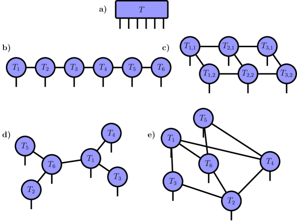
Figure 1: Example tensor network states (TNSs) as decompositions of an order $6$ tensor $T$. a) Single tensor $T$, b) a matrix product state (MPS) or tensor train (TT) decomposition of $T$, c) a projected entangled pair state (PEPS) or tensor product state (TPS) decomposition of $T$, d) a tree tensor network (TTN) or hierarchical Tucker (HT) decomposition of $T$, and e) a generic tensor network state (TNS) decomposition of $T$. Note that here we depict cases where all tensors have one external index, but in general tensors of a TNS can have zero or more than one external index, corresponding to the decomposition of an order $L$ tensor into a number of tensors not equal to $L$.

In this work we will demonstrate a new, systematic way to gauge a generic TNS. In general, a gauge transformation of a TNS involves a modification of the site tensors which leaves the overall representation unchanged, i.e. when contracting the full network the result is independent of the transformation. Most commonly, such a transformation involves inserting resolutions of the identity matrix $X_{e}^{-1}X_{e}=\mathbb{I}_{e}$, where $X_{e}$ is an invertible matrix, on each edge $e$ of the TNS and absorbing the matrices $X_{e}^{-1}$ and $X_{e}$ into the incident tensors $T_{v}$.

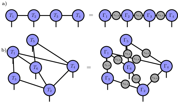
Figure 2: Examples of TNS in the Vidal gauge. a) MPS and its equivalent form in the Vidal gauge, and b) arbitrary TNS and its equivalent form in the Vidal gauge. Within the Vidal gauge, each tensor $\Gamma_{v}$ obeys the isometry condition defined by Eqs. (1) and (2).

Our work systematically identifies the gauge transformation necessary to bring a generic TNS into a gauge commonly used in the tensor network literature. In the case of tree topologies, it is commonly referred to as the ‘canonical form’ or ‘Vidal gauge’ [66, 67, 79, 74, 75, 94, 97, 96], while for general tensor networks it is the gauge implicitly used in the ‘simple update’ algorithm [119, 139, 122] and has been called the ‘super-orthogonal’ [132] or ‘quasi-canonical’ [123, 113] gauge. In this work, we will refer to it as the ‘Vidal gauge’ for both tree tensor networks and more general (loopy) tensor networks. This gauge involves a TNS with tensors $\Gamma_{v}$ on the vertices of the network and non-negative diagonal bond tensors $\Lambda_{e}$ on the edges of the network. A few examples of TNS in the Vidal gauge are illustrated in Fig. 2. Importantly, within the Vidal gauge, site tensors are ‘isometric’ upon absorbing all but one of their incident bond tensors. Specifically, by first defining the tensor

$$\leavevmode\hbox{$\vbox{\hbox{\resizebox{}{}{{\leavevmode\hbox{\set@color{}}}}}}$}\quad,$$ (1)

this isometric property can be expressed as

$$\leavevmode\hbox{$\vbox{\hbox{\resizebox{}{}{{\leavevmode\hbox{\set@color{}}}}}}$}\quad,$$ (2)

where ^∗ denotes complex conjugation and the right-hand side of Eq. (2) represents the identity matrix (provided there is an appropriate normalization on $\Gamma_{v}$ and $\Lambda_{e}$). The open indices in Eq. (2) are directed along the edge between $v$ and one of its $d$ neighbors $v_{i}$. The Vidal gauge can be defined for an arbitrary (finite or infinite) TNS and the bond tensors can be used to provide a rank-one approximation of the environment in a general loopy network — allowing rapid, approximate local updates to be performed on the TNS. When the TNS has a tree structure, the Vidal gauge allows one to define an exact reduced, orthogonal basis at any site in the network. We will introduce a new method for transforming a TNS into the Vidal gauge using belief propagation, independent of the network structure. The essential steps are outlined in Fig. 3 and in the following we will provide the explicit details.

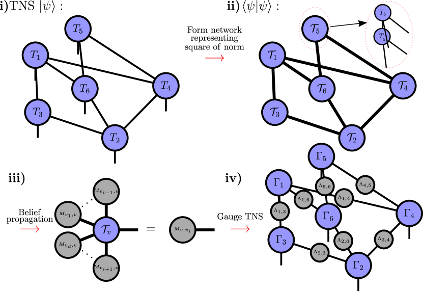
Figure 3: Steps of our belief propagation gauging routine. Starting with a TNS $|\psi\rangle$ the corresponding tensor network representing the square of the norm of the TNS $\langle\psi|\psi\rangle$ is formed. We emphasize that in practice it may be more efficient to keep the tensors in the bra and ket separate and not explicitly contract over the site indices ahead of time (shown by the expanded view of the ringed vertex $\mathcal{T}_{5}$ of the norm network in ii)). Belief propagation is then performed on this network and the fixed point message tensors are used to bring the original TNS into the Vidal gauge. In Section 3.5, we describe a generalization of this procedure to the case where the site tensors $T_{v}$ of the original network are replaced by sets of tensors. In this case the BP gauging routine is run on a partitioned tensor network comprised by groups of tensors associated with each vertex $v$.

2.2 Belief propagation for tensor network states

In order to present our gauging routine we will first introduce the belief propagation (BP) method. BP is a well-established technique for approximating the marginals of the probability distributions of graphical models [141, 142, 143, 144, 154] and has recently been adapted and generalized to tensor networks [145, 149, 150, 146]. Here, we will describe the technique in the context of a ‘closed’ tensor network, which is a tensor network where there are no external indices and thus its contraction yields a scalar. In our context, the closed network is formed as the square of a TNS — this network is composed of pairs of site tensors $T_{v}$ and their conjugates $T_{v}^{*}$. We will often denote this pair of tensors with the shorthand notation $\mathcal{T}_{v}$, and refer to this closed network as the ‘norm network’ of the TNS. For instance, the norm network of a $3\times 2$ TNS is

$$\leavevmode\hbox{$\vbox{\hbox{\resizebox{}{}{{\leavevmode\hbox{\set@color{}}}}}}$},$$ (3)

where, for efficiency purposes, it is typically advisable to not explicitly contract the two layers together but store the norm network as the structure on the left-hand side of Eq. (3).

We define a set of ‘message tensors’ of a given norm network $\{M_{e},M_{\bar{e}}\}$ for each edge $e$, where $\bar{e}$ denotes the reverse of an edge $e$. We will also use the notation $M_{v,v_{i}}$, which denotes the message tensor directed along the edge from vertex $v$ to its neighbor $v_{i}$. The indices of $M_{v,v_{i}}$ match the indices shared by $\mathcal{T}_{v}$ and $\mathcal{T}_{v_{i}}$. In general, the direction of the edge is important and $M_{e}=M_{v,v_{i}}\neq M_{\bar{e}}=M_{v_{i},v}$. A set of self-consistent equations is defined for the message tensors:

$$M_{v,v_{i}}=\left(\prod_{j\in\{1,\dots,i-1,i+1,\dots,d\}}M_{v_{j},v}\right)\mathcal{T}_{v},$$ (4)

where multiplication of two tensors implies a contraction over any common indices they share. We use the set $N(v)=\{v_{1},v_{2},...,v_{d}\}$ to denote the $d=|N(v)|$ neighbors of $v$, and the product in Eq. (4) runs over all neighbors of $v$ exluding $v_{i}$. This equation can be expressed diagrammatically as

$$\leavevmode\hbox{$\vbox{\hbox{\resizebox{}{}{{\leavevmode\hbox{\set@color{}}}}}}$}\quad.$$ (5)

Again we emphasize it is generally more efficient to treat $\mathcal{T}_{v}$ ‘lazily’ when performing the message tensor update, i.e. as the uncontracted pair $T_{v}$ and $T^{*}_{v}$. Additionally, it is straightforward to generalize to the case where $T_{v}$ (and $T^{*}_{v}$) are replaced by sets of tensors associated with the vertex $v$, which corresponds to a case of BP but with larger groups or partitions of tensors representing $\mathcal{T}_{v}$. See Section 3.5 for more details and examples of more general TNS structures.

After initializing the message tensors, one can iterate the set of equations defined by Eq. (5) in an attempt to converge them. In Section 3 we explain how convergence can be measured, along with numerical results on the convergence of BP for various example networks. The converged message tensors then form an approximation for the exact environment for a given vertex $v$. The exact environment would be the result of contracting the full network surrounding $\mathcal{T}_{v}$: an operation which, for a general network, scales exponentially in the size of the network [124, 48, 168]. Mathematically, the message tensor approximation for the environment can be stated as

$$\prod_{w\neq v}\mathcal{T}_{w}\approx\lambda_{v}\prod_{v_{i}\in N(v)}M_{v_{i},v},$$ (6)

where the product on the left-hand side runs over all vertices in the network excluding $v$ and the right-hand side runs over the set $N(v)=\{v_{1},v_{2},...,v_{d}\}$ of $d=|N(v)|$ neighbors of $v$. The scalar $\lambda_{v}$ is dependent on the normalization of the message tensors and the tensors of the TNS. For illustration, in a $6$-site network, an example of Eq. (6) would be

$$\leavevmode\hbox{$\vbox{\hbox{\resizebox{}{}{{\leavevmode\hbox{\set@color{}}}}}}$}\quad.$$ (7)

This can be used to approximate expectation values (e.g. Eq. 37) or approximately contract a gate with a TNS (e.g. Fig. 5b). Importantly, if the network forms a tree and the message tensors have converged to a fixed point, i.e. they satisfy Eq. (4), then Eq.(6) is exact and no longer an approximation. Next, we will show how belief propagation can be used to transform an arbitrary tensor network state into the Vidal gauge, starting with a review of gauging matrix product states (MPSs) from the perspective of belief propagation.

2.3 Using belief propagation to gauge a matrix product state

We will start by reviewing how to transform a matrix product state (MPS) or tensor train (TT) into the canonical form or Vidal gauge [66, 67, 75, 6], but reframed in the language of belief propagation. A MPS is a tensor network with a linear or path graph topology. Labelling the vertices as $v\in\{1,...,L\}$, each vertex $v$ has neighbors $N(v)=\{v-1,v+1\}$ in the bulk of the chain:

$$\leavevmode\hbox{$\vbox{\hbox{\resizebox{}{}{{\leavevmode\hbox{\set@color{}}}}}}$}\quad.$$ (8)

Let us first take a given MPS and combine it with its conjugate to create the closed tensor network which represents the square of its norm (the ‘norm network’):

$$\leavevmode\hbox{$\vbox{\hbox{\resizebox{}{}{{\leavevmode\hbox{\set@color{}}}}}}$}\quad.$$ (9)

The self-consistent BP equations are then

$$\leavevmode\hbox{$\vbox{\hbox{\resizebox{}{}{{\leavevmode\hbox{\set@color{}}}}}}$}\quad,$$ (10)

along with corresponding message tensor updates for $\{M_{v,v-1}\}$, where we visualize the equations both in terms of $T_{v}$ explicitly or grouped into $\mathcal{T}_{v}$ (though in practice keeping it in terms of $T_{v}$ is generally more efficient). Importantly, if the initial message tensors used are positive semidefinite then the self-consistency equations are guaranteed to preserve this property at each step. Due to the simple topology of the network, successively applying Eq. (10) from left to right (or right to left for computing $\{M_{v,v-1}\}$) will give convergence of the message tensors after a single update of each message tensor — recovering a standard method for contracting a MPS [6]. Because the network is a tree, these message tensors form an exact representation of the environments of the local norm tensors $\mathcal{T}_{v}$. After reaching this fixed point, it follows from Eq. (10) that we now have a set of message tensors $\{M_{e},M_{\bar{e}}\}$ over the edges $e$ — and their reverses $\bar{e}$ — of the norm network where

    (11)

which means that $M^{\frac{1}{2}}_{v-1,v}T_{v}M^{-\frac{1}{2}}_{v,v+1}$ is an isometric tensor. This corresponds to transforming the MPS into the orthogonal or mixed canonical gauge [6, 2]. We have defined the square root of a message tensor $M_{e}=\left(M^{\frac{1}{2}}_{e}\right)^{\dagger}M^{\frac{1}{2}}_{e}$ by performing the eigendecomposition $M_{e}=U_{e}^{\dagger}D_{e}U_{e}$ and letting $M^{\frac{1}{2}}_{e}=D_{e}^{\frac{1}{2}}U_{e}$, where $U_{e}$ is unitary and $D_{e}$ is a positive semidefinite diagonal matrix. Additionally, $M^{-\frac{1}{2}}_{e}=U_{e}^{\dagger}D_{e}^{-\frac{1}{2}}$ where a pseudoinverse may be required if small eigenvalues are present. Note that this definition of the square root is not unique and has a unitary degree of freedom, i.e. we can just as well use $M^{\frac{1}{2}}_{e}=W_{e}^{\dagger}D_{e}^{\frac{1}{2}}U_{e}$ for any unitary $W_{e}$.

Now, using the message tensors found from BP we take the following singular value decomposition (SVD)

$$\leavevmode\hbox{$\vbox{\hbox{\resizebox{}{}{{\leavevmode\hbox{\set@color{}}}}}}$}\quad,$$ (12)

which is an approximation if singular values of the bond tensor $\Lambda_{v,v+1}$ are discarded and its dimensions reduced, which amounts to an optimal truncation of the MPS rank or bond dimension according to the 2-norm. The $U$ and $V$ tensors are isometric and satisfy the following properties

$$\leavevmode\hbox{$\vbox{\hbox{\resizebox{}{}{{\leavevmode\hbox{\set@color{}}}}}}$}\quad,$$ (13)

$$\leavevmode\hbox{$\vbox{\hbox{\resizebox{}{}{{\leavevmode\hbox{\set@color{}}}}}}$}\quad,$$ (14)

a fact indicated by their semistadium shape. We define the following $\Gamma_{v}$ tensors as

$$\leavevmode\hbox{$\vbox{\hbox{\resizebox{}{}{{\leavevmode\hbox{\set@color{}}}}}}$}\quad,$$ (15)

and the $\Lambda_{v,v+1}$ bond tensors as

$$\leavevmode\hbox{$\vbox{\hbox{\resizebox{}{}{{\leavevmode\hbox{\set@color{}}}}}}$}\quad.$$ (16)

These can be directly used to construct a version of the original matrix product state in the Vidal gauge. Specifically, we have transformed our original MPS to a MPS in the Vidal gauge by the following sequence of operations:

    (17)

with equality occurring if no truncation is done during the SVD. Each local tensor in the Vidal gauged MPS now approximately satisfies

$$\leavevmode\hbox{$\vbox{\hbox{\resizebox{}{}{{\leavevmode\hbox{\set@color{}}}}}}$}\quad,$$ (18)

$$\leavevmode\hbox{$\vbox{\hbox{\resizebox{}{}{{\leavevmode\hbox{\set@color{}}}}}}$}\quad,$$ (19)

where again equality occurs if no singular values are discarded during the SVD. These identities can be proven by: i) substituting the expressions for $\Lambda_{v,v+1}$ and $\Gamma_{v}$ in Eqs. (15) and (16) into Eqs. (18) and (19), ii) utilizing that $U^{\dagger}_{v,v+1}U_{v,v+1}$ and $V^{\dagger}_{v,v+1}V_{v,v+1}$ act as approximate resolutions of the identity up to the singular values truncated in Eq. (12), and iii) using the result in Eq. (11) and the isometric constraints Eqs. (13) and (14). The method we have described above can be straightforwardly applied to a tree tensor network state (TTNS), where it is also possible to find the fixed point message tensors in a single update by performing the message tensor updates in a particular sequence. Once in the Vidal gauge, optimal truncations according to the 2-norm can be performed of the MPS/TTNS to lower the bond dimension (i.e. by truncating according to the singular values as shown in Eq. (12)).

2.4 Using belief propagation to gauge a tensor network state

We will now generalize the method for transforming a MPS into the Vidal gauge described in the previous section to demonstrate how to transform a generic tensor network state into the Vidal gauge without any assumptions of a tree-like structure, as illustrated in Fig. 3. Again, one first converges the self-consistent BP equations — see Eq. (5) — over the norm network of the TNS, to obtain the set of message tensors $\{M_{e},M_{\bar{e}}\}$. Unlike with tree tensor networks, however, in general there is no direct way to converge the message tensors after a single update and so one must generally rely on iterating the self-consistent BP equations. Upon convergence of these equations, the following identity is true on every edge of the network:

$$\leavevmode\hbox{$\vbox{\hbox{\resizebox{}{}{{\leavevmode\hbox{\set@color{}}}}}}$}\quad,$$ (20)

or in other words if the tensors on the top half of the left-hand side are contracted together they form an isometric tensor and the tensors on the bottom half form its conjugate. This relationship can be derived from Eq. (5) by taking the square roots of the message tensors and inverting the square root message tensors on the right-hand side of the equation. Just as for the case of a MPS we define the following:

$$\leavevmode\hbox{$\vbox{\hbox{\resizebox{}{}{{\leavevmode\hbox{\set@color{}}}}}}$}\quad,$$ (21)

$$\leavevmode\hbox{$\vbox{\hbox{\resizebox{}{}{{\leavevmode\hbox{\set@color{}}}}}}$}\quad,$$ (22)

$$\leavevmode\hbox{$\vbox{\hbox{\resizebox{}{}{{\leavevmode\hbox{\set@color{}}}}}}$}\quad.$$ (23)

The $U_{v,v_{i}}$ and $V_{v_{i},v}$ matrices again possess the isometric properties described in Eqs. (13) and (14). We can then transform the TNS into the Vidal gauge from the fixed point message tensors and the original TNS using Eqs. (22) and (23). Such a transformation corresponds to: i) inserting the resolution of identity $\mathbb{I}_{e}=M^{-\frac{1}{2}}_{e}M^{\frac{1}{2}}_{e}M^{\frac{1}{2}}_{\bar{e}}M^{-\frac{1}{2}}_{\bar{e}}$ along the edges of the original TNS, ii) performing the SVD in Eq. (21), and iii) absorbing the inverse square root message tensors $M^{-\frac{1}{2}}_{e}$ along with the $U_{e}$ and $V_{e}$ tensors obtained from the SVD onto the on-site tensors $T_{v}$, analogous to the steps shown in Eq. (17) for gauging a MPS. For the example of a $6$-site TNS the result is

$$\leavevmode\hbox{$\vbox{\hbox{\resizebox{}{}{{\leavevmode\hbox{\set@color{}}}}}}$}\quad,$$ (24)

which, if no truncation is done during the SVD, becomes an equality. Note that SVD truncations are not optimal for loopy networks, and are only valid up to the BP approximation (i.e. can be close to optimal for TNS with tree-like correlations).

Assuming the message tensors used satisfy the fixed point criterion in Eq. (5) and no truncation is done then the right-hand side of Eq. (24) is provably in the Vidal gauge: Eqs. (1) and (2) are valid along all edges of the network. The proof of this is essentially analogous to that for a MPS and can be achieved by i) substitution of the expressions for $\Gamma_{v}$ and $\Lambda_{e}$ into the tensor network in the Vidal gauge (such as the right-hand side of Eq. (24)), ii) utilizing that $U^{\dagger}_{e}U_{e}$ and $V^{\dagger}_{e}V_{e}$ act as approximate resolutions of the identity up to the singular values truncated in Eq. (21), and iii) invoking the identity in Eq. (20) and the isometric constraints Eqs. (13) and (14).

Eqs. (21), (22), and (23) define an algorithm for bringing an arbitrary TNS into the Vidal gauge. This can be summarized by the following steps:

The belief propagation (BP) gauging routine

• Start with a TNS consisting of site tensors $\{T_{v}\}$. Form the closed network corresponding to the square of the norm of the TNS.

• Initialize the belief propagation message tensors $\{M_{e},M_{\bar{e}}\}$ of the normed network to arbitrary, positive definite matrices.

• Perform iterations of belief propagation, where each iteration corresponds to an update of each message tensor via Eq. (5), up to some stopping criteria.

• Gauge the TNS with the resulting message tensors via Eqs. (21), (22), and (23). This yields the TNS in the Vidal gauge with site tensors $\{\Gamma_{v}\}$ and bond tensors $\{\Lambda_{e}\}$.

The less truncation performed during the SVD in Eq. (21) and the more iterations of belief propagation performed, the closer the tensors in the TNS will be to satisfying the isometric conditions in Eqs. (1) and (2). We refer to our algorithm as belief propagation gauging or BP gauging for short.

Note the very close similarity to the steps of BP gauging, such as the definitions of $\Gamma_{v}$ and $\Lambda_{e}$ in Eqs. (21), (22), and (23), to the steps of the gauging method introduced in Refs. [132, 134], which also transforms a general tensor network state into the Vidal gauge and which we refer to as ‘eager gauging’. A key distinction from that method is that in BP gauging, the gauge transformation is only performed once at the end, after belief propagation is performed on the original network to a desired level of convergence of the message tensors. In contrast, gauge transformations are performed at every iteration in eager gauging. In fact, in the language of belief propagation, the eager gauging method can be interpreted as alternating steps of running an iteration of belief propagation on the symmetric gauge of the network (defined in Section 2.6 below) and then performing the gauge transformation defined in Eqs. (21), (22), and (23) on the updated message tensors. It turns out that for the sake of gauging a tensor network into the Vidal gauge, performing gauge transformations after each step of BP besides the final step is extraneous and can be avoided altogether. We summarize the eager gauging algorithm defined in Refs. [132, 134] in the language of BP in Appendix B. Numerical results in Sec. 3.2 corroborate that the gauging methods have the same convergence properties but that BP gauging is faster because it requires fewer operations at each iteration.

2.5 Using square root belief propagation to gauge a tensor network state

An alternative standard procedure for gauging a MPS or TTN into the orthogonal or canonical form involves taking QR decompositions (or some other orthogonal decomposition) of what would be, in the language of belief propagation, the square roots of the message tensors absorbed into the site tensors [6]. This amounts to performing the MPS message tensor update shown in Eq. (10) using a QR decomposition $M^{\frac{1}{2}}_{v-1,v}T_{v}=Q_{v,v+1}M^{\frac{1}{2}}_{v,v+1}$ (or $T_{v}M^{\frac{1}{2}}_{v+1,v}=M^{\frac{1}{2}}_{v-1,v}Q_{v,v-1}$ in the case of a right to left update). After squaring, the resulting message tensors would still satisfy the relations in Eqs. (10) and (11). This has the advantage that the square root message tensors can be found to higher precision, though at the cost of performing QR decompositions. An analogous ‘square root’ belief propagation update can be performed for arbitrary tensor networks [169] using QR decompositions to perform square root message tensor updates:

$$\leavevmode\hbox{$\vbox{\hbox{\resizebox{}{}{{\leavevmode\hbox{\set@color{}}}}}}$}\quad,$$ (25)

which can be iterated to find a set of fixed point square root message tensors $\left\{M^{\frac{1}{2}}_{e},M^{\frac{1}{2}}_{\bar{e}}\right\}$. These can then be directly used for transforming the network into the Vidal gauge with Eqs. (21), (22), and (23). As in the MPS case this can have the advantage of providing higher numerical precision. To avoid some of the higher cost due to performing QR decompositions (or some other orthogonal decomposition), one can first converge using the standard message tensor updates from Eq. (5) and then switch to the square root message tensor update in Eq. (25), similar to procedures formulated for gauging MPS [11, 159, 2]. Note that this is closely related to the ‘simple update gauging’ method which we review in Appendices A and B. Specifically, a square root BP update step is analogous to steps i-iii) of Fig. 11 but, unlike in simple update gauging, regauging is only performed in the final iteration after the square root message tensors are converged. This avoids repeatedly performing gauge transformations at each message tensor update, which is done at every bond update in simple update gauging (steps iv-viii) of Fig. 11).

2.6 The symmetric gauge

Here we will introduce a useful gauge for a TNS that is very closely related to the Vidal gauge. Specifically, given a TNS in the Vidal gauge, it is straightforward to define the square roots of the bond tensors:

$$\leavevmode\hbox{$\vbox{\hbox{\resizebox{}{}{{\leavevmode\hbox{\set@color{}}}}}}$}\quad,$$ (26)

and absorb them onto the site tensors $\Gamma_{v}$:

$$\leavevmode\hbox{$\vbox{\hbox{\resizebox{}{}{{\leavevmode\hbox{\set@color{}}}}}}$}\quad,$$ (27)

using the example of a degree $d=4$ tensor above. We can then recover a TNS without bond tensors:

$$\leavevmode\hbox{$\vbox{\hbox{\resizebox{}{}{{\leavevmode\hbox{\set@color{}}}}}}$}\quad.$$ (28)

This gauge has been introduced previously in the tensor network literature [119, 134, 153]. In the following, we will refer to this as the ‘symmetric gauge’. An important aspect of this form is that if we have a state in the Vidal gauge, then transforming to the symmetric gauge and running belief propagation will yield the fixed point message tensors $\{M_{e}=M_{\bar{e}}=\Lambda_{e}\}$. In other words, for a TNS in the symmetric gauge, the message tensors are the same in both directions along a given edge $e$, and equivalent to the positive diagonal bond tensors $\{\Lambda_{e}\}$ of the Vidal gauge of the same TNS. This property of the symmetric gauge was previously pointed out in Ref. [153]. The proof of this can be done by writing down the self-consistency equation for the message tensors of the norm network in the symmetric gauge (Eq. (5)), substituting in the definition of the symmetric gauge tensors (Eq. (27)), and observing that it is equivalent to the Vidal gauge isometric condition defined in Eqs. (1) and (2) if $M_{e}=M_{\bar{e}}=\Lambda_{e}$.

3 Applications and benchmarks of belief propagation gauging

3.1 Quantifying the distance to the Vidal gauge of a tensor network state

In order to detail our numerical results it will be important to quantify how closely a state in the Vidal gauge actually obeys the isometry condition in Eqs. (1) and (2). This is directly dependent on how close the message tensors used to gauge the original state are to their fixed point and, in a general numerical implementation, they will only be approximately at the fixed point and thus the isometry condition in Eqs. (1) and (2) will only be obeyed approximately.

To treat this we introduce a new quantifier $\mathcal{C}$ which we refer to as the ‘distance to the Vidal gauge’. We will use this to measure the effectiveness of various algorithms, including ours, at bringing a TNS into the Vidal gauge. Given a TNS in the Vidal gauge — i.e. consisting of bond tensors $\{\Lambda_{e}\}$ and site tensors $\{\Gamma_{v}\}$ — $\mathcal{C}$ is defined as

$$\leavevmode\hbox{$\vbox{\hbox{\resizebox{}{}{{\leavevmode\hbox{\set@color{}}}}}}$}\quad,$$ (29)

where we have introduced the squares of the bond tensors

$$\leavevmode\hbox{$\vbox{\hbox{\resizebox{}{}{{\leavevmode\hbox{\set@color{}}}}}}$}\quad.$$ (30)

Equation (29) essentially measures the average degree to which Eqs. (1) and (2) are satisfied by the tensors in the TNS. Here, $||A-B||_{1^{\prime}}=\left|\left|\frac{A}{{\rm Tr}(A)}-\frac{B}{{\rm Tr}(B)}\right|\right|_{1}$ and $||M||_{1}$ represents the trace norm of a matrix $M$. Both matrices in Eq. (29) are scaled to trace unity in order to remove any dependence of $\mathcal{C}$ on the normalization of the network.

Importantly, one can accurately determine the order of magnitude of $\mathcal{C}$ — which we denote with $O(\mathcal{C})$ — by assessing the distance of the message tensors found via belief propagation from their fixed point. This allows one to target a precscribed $O(\mathcal{C})$ in belief propagation gauging while avoiding having to explicitly gauge the state and compute the isometries to measure $\mathcal{C}$ at every step of belief propagation. Specifically,

$$O\left(\mathcal{C}^{(n)}\right)\approx\frac{1}{2|E|}\sum_{v}\sum_{i=1}^{|N(v)|}\left|\left|M^{(n-1)}_{v,v_{i}}-M^{(n)}_{v,v_{i}}\right|\right|_{1^{\prime}},$$ (31)

where $n$ is the current iteration of BP. This can be derived using Eqs. (5), (21), (22), and (23) and comparing to Eq. (29). This allow us to use BP to gauge a TNS to a prescribed order of magnitude of $\mathcal{C}$ without any significant computational overhead from checking the value of $\mathcal{C}$.

3.2 Accelerating tensor network gauging with belief propagation

Here we perform numerical simulations using the ITensorNetworks.jl package [170], demonstrating the efficacy of the BP gauging method for gauging general tensor network states. For a given TNS we will repeatedly run iterations of belief propagation on the corresponding norm network. We expect to observe the message tensors found after an increasing number of iterations will bring the TNS closer and closer to the Vidal gauge, i.e. they can be used to transform the TNS to a state with an increasingly small value of $\mathcal{C}$ defined in Section 3.1. We will benchmark the convergence of $\mathcal{C}$ with belief propagation iterations against existing algorithms for bringing a TNS into the Vidal gauge.

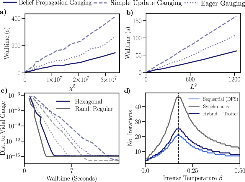
Figure 4: a-b) Time to reach $\mathcal{C}=10^{-10}$ for a random TNS — with tensor elements drawn from the normal distribution of mean $0$ and standard deviation $1$ — of bond dimension $\chi$ on an $L\times L$ square lattice. a) Scaling with $\chi^{5}$ for $L=12$. The plot ranges to $\chi=32$ where we see that eager gauging and simple update gauging take $1.82$ and $2.81$ times longer than belief propagation gauging respectively. b) Scaling with $L^{2}$ for $\chi=15$. The plot ranges to $L=35$ where we see that eager gauging and simple update gauging take $1.75$ and $2.63$ times longer than belief propagation gauging respectively. c) Distance to the Vidal gauge $\mathcal{C}$ versus walltime for gauging a random tensor network state with elements drawn from the normal distribution of mean $0$ and standard deviation $1$. The bond dimension of the TNS is $\chi=20$ and two lattices are shown: the hexagonal TNS for $10$ rows and $10$ columns of hexagons, and a $200$ site random regular graph of fixed degree $3$. In plots a-c) different line styles correspond to different gauging methods (with the legend at the top of the figure) and all walltimes are in seconds. Iterations of each algorithm are performed using a fixed Suzuki-Trotter decomposition-inspired schedule of updates over the edges of the TNS (see main text for more details). d) Number of iterations required to reach $\mathcal{C}=10^{-8}$ for the TNS corresponding to the square root of the classical Ising partition function (which has bond dimension $2$) versus inverse temperature $\beta$. A longitudinal field of $h=0.5$ is included. Results are for a $20\times 20\times 20$ cubic lattice. Different colors correspond to different update schedules for the message tensors in a given iteration - with further details in the main text - and the total walltime is directly proportional to the number of iterations.

The first of these algorithms we term simple update gauging [119, 123, 153]. This routine starts with a TNS in the Vidal gauge and lowers the corresponding value of $\mathcal{C}$ by repeatedly performing a simple update with ‘identity’ gates on the edges of the network — the simple update procedure is pictured in Fig. 5, with more extensive details in Appendices A and B. The second algorithm, which we term eager gauging [132, 134], is very closely related to our algorithm, as we discussed at the end of Section 2.4. Instead of an iteration of BP, each iteration of eager gauging involves alternating iterations of BP interspersed with gauge transformations. In Appendix B we provide explicit details of the steps involved in both the eager and simple update gauging routines.

The runtime and convergence of these algorithms is dependent on the order in which the message tensors are updated in a given iteration, which is called the schedule. This schedule can either be ‘synchronous’ or ‘asynchronous’, also referred to as ‘serial’ or ‘sequential’ schedules. In the case of synchronous schedules, all message tensors (or site and bond tensors in the case of simple update or eager gauging) are updated at once given their current state. For asynchronous or serial schedules, message tensors (or site and bond tensors) are updated one at a time, so that message tensor updates can make use of previously updated message tensors within an iteration. Naturally, serial scheduling implies that the order of edges to perform updates over is important while for synchronous scheduling it is not. When a serial schedule is chosen well, it can require fewer message tensor updates to converge [171, 172], though synchronous schedules allow for performing message tenors updates simultaneously in parallel (something which we do not take advantage of in our current benchmarks) . In order to properly compare the various tensor network gauging algorithms, we use a consistent schedule across the different algorithms. In particular, we use a hybrid synchronous-serial schedule where we split the edges of the TNS into a minimum number of groups where edges in the same group don’t share common vertices. This corresponds to the grouping of gates/edges in a Suzuki-Trotter decomposition [173] of a nearest-neighbor Hamiltonian on the graph of the tensor network. In a given iteration, we then perform serial updates between edge groups but synchronous updates within the same group. In the case of BP or eager gauging, when a given edge of the TNS appears in the update schedule, we perform a synchronous update of the forward and backward message tensors via Eq. (4).

Fig. 4 displays our benchmark of these gauging routines for a variety of different tensor network states. Specifically, in Fig. 4a-b we consider a square lattice TNS composed of tensors with random elements that are normally distributed around zero. We show how the time to reach $\mathcal{C}\leq 10^{-10}$ scales with system size and bond dimension. We can see that BP gauging is faster than both simple update gauging and eager gauging for all bond dimensions and system sizes. As expected, all of the methods have a dominant scaling of $\mathcal{O}(N\chi^{z+1})$, where $\chi$ is the bond dimension, $z$ is the largest coordination number in the network, and $N$ is the number of sites in the network with coordination number $z$ (where $N=L^{2}$ in Fig. 4a-b for an $L\times L$ square lattice).

We can explain the performance improvement of BP gauging over the other methods based on counting the number of operations that scale as $O(\chi^{z+1})$ in each iteration of the different algorithms. We should emphasize, for a fixed update schedule, the number of iterations required by each algorithm to reach a given $\mathcal{C}$ is identical as each step of the algorithm updates the state in an analogous way, and all of them can be viewed as variations of belief propagation. Thus the performance is entirely based on the timing of a single iteration of each algorithm, up to the fact that the final step of BP gauging will involve an additional step of gauging using the fixed point message tensors. Each iteration is dominated by a number of operations that scale with the bond dimension $\chi$ as $O(\chi^{z+1})$ in the limit of large $\chi$. The extraneous gauge transformations at each iteration of eager gauging means that there are approximately $z$ extra tensor contractions that are of $O(\chi^{z+1})$ which are not performed by BP gauging.

In simple update, in the limit of large $\chi$ the cost of each iteration is dominated by tensor contractions that scale as $O(\chi^{z+1})$ as well as QR decompositions that scale as $O(\chi^{z+1})$. Like eager gauging, simple update gauging has on the order of $z$ extra tensor contractions that scale as $O(\chi^{z+1})$ compared to BP gauging. Additionally, a QR decomposition of $O(\chi^{z+1})$ generally has a higher constant prefactor than a tensor contraction of $O(\chi^{z+1})$, which also contributes to the higher runtime per iteration compared to BP gauging.

In Fig. 4c we consider random TNSs (again, with normally distributed elements) of different geometries: a hexagonal lattice grid consisting of $10\times 10$ rows and columns of hexagons and a random regular graph of $200$ sites and degree $z=3$. The distance to the Vidal gauge decreases exponentially with walltime in each algorithm, with BP gauging displaying the largest rate of decay (due to the faster speed of each iteration as argued above).

Finally, in Fig. 4d, we construct the TNS corresponding to the square root of the partition function of the classical Ising model with a longitudinal field on a $20\times 20\times 20$ cubic lattice (see Refs. [174, 149] for explicit details on how to construct this state for an arbitrary network). We focus solely on BP gauging and consider the effect of different update schedules for the convergence of the TNS, which has bond dimension $\chi=2$, to the Vidal gauge. All schedules take the longest to converge at the critical point due to the long-range correlations present in the state. We compare three different schedules: i) fully synchronous updates, ii) the hybrid synchronous-serial schedule inspired by the Suzuki-Trotter decomposition described above, and iii) serial updates based on our custom sequence. We note that the worst performance is observed for fully synchronous update schedules which is consistent with that seen in the BP literature [171, 172]. Here, we find our custom schedule — which is closely related to schedules proposed in [175, 176, 177] — is best for the performance of BP gauging. It is based on finding a forest cover of the network [178], performing depth first search (DFS) to find an update sequence for each of the trees in the forests, and concatenating the resulting sequences to get a full sequence for the network. We use a breadth first search to construct the spanning trees which make up the forests which typically finds comb-like trees on grid graphs. This is similar to the spanning trees considered in [175, 176, 177]. For a tree tensor network there is only one forest in the forest cover and one tree within that forest. Thus the schedule reproduces the known result that running BP and finding the Vidal gauge only requires a single iteration of BP. For a loopy network, an iteration of BP involves iterating through the trees of the forest cover. We should also point out a wide range of different serial schedules have also been proposed in the BP literature with various advantages and disadvantages [175, 176, 177, 172] — comparing these to each other and our custom schedule in the context of tensor network gauging is a topic of future research.

3.3 Approximate gate application with belief propagation

A common method for performing gate evolution of a TNS is the simple update (SU) method [119, 115, 179, 180, 181], which we summarize in Fig. 5a and Appendix A. The SU gate application method implicitly uses an approximate Vidal (or quasi-canonical/super-orthogonal) gauge. This is the routine at the heart of simple update gauging (which is equivalent to performing SU with identity gates, see Fig. 11 in Appendix A). It is based on an approximation of the environment as a product of matrices, which is exact on trees [79, 94] and can be a good approximation for systems with tree-like correlations. For systems with non-tree-like correlations, such as strongly correlated systems on regular lattices with small loop structures (like square lattices), it is commonly used to provide starting states and rank-one reference points for more demanding but accurate TNS calculations. Examples of more controlled and accurate methods for evolving or optimizing TNS are ‘full update’ gate evolution [182, 120, 122, 133, 113] and variational optimization or gradient descent [117, 183, 184, 185, 186] based on higher-rank approximations of the environment (which are commonly approximated as MPS).

Importantly, the simple update procedure can actually be performed on a tensor network state in an arbitrary gauge by using the message tensors found from belief propagation as the rank-one approximation of the environment. In Fig. 5b we summarize this procedure. This is equivalent to performing a ‘full update’ [182, 120, 122, 133, 113] with the message tensors as the environment, but the rank-one nature of the environment allows one to solve the fidelity optimization directly instead of iteratively, which is much faster in practice. We emphasize that, if the BP message tensors and Vidal gauge bond tensors are similarly accurate, simple update with BP message tensors is equivalent to performing SU in the Vidal gauge, which is summarized in Fig. 5a. In the Vidal gauge, the bond tensors act as the rank-one approximations of the environment, analagous to the role of message tensors (and in fact are just message tensors in a different gauge, which is at the heart of the BP gauging routine introduced in Section 2.4). Note that both of these routines can benefit from efficiency improvements by performing a ‘reduced tensor’ SVD (see Appendix A for explicit examples in the context of SU in the Vidal gauge, with straightforward translations of the same procedures to performing SU in arbitrary gauges with BP message tensors).

Finally, we would like to point out that repeated applications of the BP simuple update procedure over the bonds of a TNS with identity gates will transform the TNS to the symmetric gauge (defined in Section 2.6). This is analogous to simple update gauging, where repeated application of identity gates with simple update via Fig. 5a will bring a TNS into the Vidal gauge.

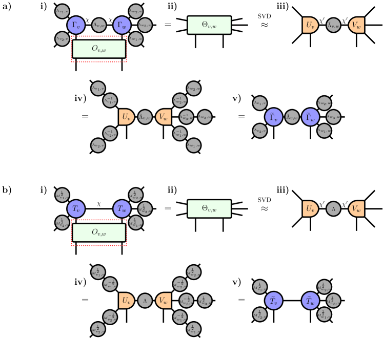
Figure 5: a) Simple update gate evolution in the Vidal gauge. i) - ii) The bond tensors and gate $O_{v,w}$ (marked by the red dotted line) are combined into a single composite tensor $\Theta_{v,w}$. ii) - iii) $\Theta_{v,w}$ is SVDd and singular values of the resulting bond tensor $\tilde{\Lambda}_{v,w}$ can be discarded in order to truncate the bond down to a desired dimension $\chi^{\prime}$. iii) - iv) Resolutions of identity, using the original bond tensors, are inserted on the exposed edges. iv) - v) The inverse bond tensors are absorbed, resulting in the updated site tensors $\tilde{\Gamma}_{v}$ and $\tilde{\Gamma}_{w}$ and the bond tensor $\tilde{\Lambda}_{v,w}$. b) The analog of simple update gate evolution using BP message tensors, equivalent to ‘full update’ gate evolution where the environment is products of message tensors. The steps are analogous to the simple update procedure for the Vidal gauge. The new message tensors on the bond $v,w$ is taken to be $\tilde{M}_{v,w}=\tilde{M}_{w,v}=\Lambda$, the diagonal tensor from the SVD whose square root is also absorbed by $U_{v}$ and $V_{w}$. a) and b) are equivalent updates of the state and represent ideal rank-one gate applications if, before applying the gates, either the state in a) is regauged using one of the Vidal gauging methods or BP is run on the state in b) to get updated fixed point message tensors. More efficient versions of these procedures (with and without the gate) are pictured in Figs. 10 and 11.

3.4 Improving the accuracy of tensor network evolution with regauging

In this section we describe an application of our new BP gauging method to improving the accuracy of TNS gate evolution with the simple update method. Other gauging methods like simple update gauging [119, 123] and eager gauging [132, 134, 114], which we have shown reach the same fixed point as BP gauging, can perform the same task (though they are potentially slower to reach the fixed point compared to BP gauging, as evidenced by our benchmarks in Section 3.2).

As demonstrated by the simple update gauging routine, if enough identity gates are applied using the simple update routine the state will converge to the Vidal gauge, where it approximately satisfies the orthogonality condition defined in Eqs. (1) and (2). For time evolution of a TNS with a Trotter circuit, in the limit of small Trotter steps and truncations, the gates are approximately identity and the gate applications act to both perform the evolution and improve the Vidal gauge orthogonality conditions of the state. However, if gates far from the identity are applied (such as in a generic quantum circuit or for large Trotter step sizes) or if significant truncation is performed during the gate evolution, the state may stray from satisfying the orthogonality conditions. This can lead to a loss in accuracy during the gate evolution because the environments aren’t the optimal rank-one environments.

To remedy this situation, one can try to find improved rank-one environments for performing the simple update gate evolution. One strategy would be to run the belief propagation (BP) tensor network contraction algorithm on the norm network of the TNS in the same spirit as Ref. [150], which focused on using BP to compute rank-one environments for calculating expectation values and performing energy optimization of tensor networks on sparse graphs. For this algorithm, one would run BP on the norm network of the state being evolved and use the fixed point message tensors as rank-one approximations of the environment in order to perform gate evolution with the ‘full update’ algorithm or BP-variant of simple update (which are entirely equivalent in the case of BP) that we show in Fig. 5b.

Based on the equivalence between the BP fixed point and the Vidal gauge that was first pointed out in Ref. [153] and further solidified by our new BP gauging algorithm, however, this is equivalent to regauging the tensor network into the Vidal gauge and then performing the simple update gate application with the regauged $\Gamma_{v}$ and $\Lambda_{e}$ tensors. This ‘regauging’ technique was (as far as we know) first proposed in [114]. In that work, the authors proposed to use what we refer to in this work as ‘eager gauging’ to regauge the network into the Vidal gauge to improve the accuracy of simple update gate evolution, but any gauging method (simple update gauging, eager gauging, or our new belief propagation gauging) can be used. This regauging can be performed at every gate application, in which case it is equivalent to performing the entire evolution with BP message tensors as the environments (either via full update or the version in Fig. 5b). Alternatively, it can be performed only when it is detected that the Vidal gauge orthogonality constraints are no longer accurate up to a certain threshold and therefore will affect the accuracy of the gate application.

We run several dynamical simulations where we apply two-site gates to a TNS in the Vidal gauge with simple update (Fig. 5a) and periodically regauge with BP gauging. This is equivalent to applying two-site gates to a TNS in an arbitrary gauge using message tensor environments (Fig. 5b), while periodically re-running belief propagation to improve the message tensors. We consider two scenarios: a) imaginary time evolution of the TNS towards the ground state of the 2D transverse field Ising model at criticality and b) repeatedly applying layers of random nearest-neighbour two-site unitary gates to the TNS. We choose 2D square lattices solely because we can use boundary MPS [117, 155] to accurately compute the energy and fidelities for moderately large lattice sizes.

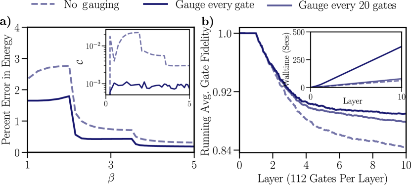
Figure 6: Imaginary and real time dynamics of a tensor network state on a 2D lattice, starting from an initial product state with neighboring spins polarized in opposite directions along the spin $z$ axis. Solid lines show evolution while performing belief propagation gauging after the application of a certain number of gates while the dashed line shows the case where no gauging is performed. a) Percent difference between energy of the 2D TNS during imaginary time evolution under $U=\exp(-\Delta\beta H)$ in Eq. (33) and energy found via DMRG on a MPS ansatz with a bond dimension of $500$. The Hamiltonian $H$ is the 2D transverse field Ising model with a field strength of $h=3.0$. The lattice is size $10\times 10$. Imaginary time steps of $\Delta\beta=0.25,0.15$, and $0.1$ are used for $8$, $10$, and $15$ applications of $U(\Delta\beta)$ respectively. The 2D TNS is limited to a maximum bond dimension of $\chi=2$ and the energy is calculated via boundary MPS [117, 155] with a MPS bond dimension of $D=10$; this is enough to achieve convergence in expectation values. For the solid line, the gauging routine targets $O(\mathcal{C})=10^{-3}$. Inset) Distance to Vidal gauge versus imaginary time. b) Average gate fidelity (Eq. (35)) for an $8\times 8$ lattice and applying cross-hatched layers of random two-site unitaries with the bond dimension limited to $\chi=4$. Fidelities are calculated using boundary MPS with a maximum dimension of $D=10$. For the solid lines, the gauging routine targets $O(\mathcal{C})=10^{-3}$ and uses a serial update schedule for each belief propagation based on forest covers of the lattice and depth first search (see main text for further details). Each layer consists of $112$ gates. Inset) Walltime, in seconds, of the different simulations.

For imaginary time evolution, the Hamiltonian on an $L\times L$ open boundary lattice reads

$$H=\sum_{\langle v,v^{\prime}\rangle}\sigma^{x}_{v}\sigma^{x}_{v^{\prime}}-g\sum_{v}\sigma^{z}_{v}=\sum_{\langle v,v^{\prime}\rangle}h_{v,v^{\prime}}+\sum_{v}h_{v^{\prime}},$$ (32)

where the first summation runs over the nearest neighbour pairs in the lattice and the second runs over all the sites of the lattices. The propagator is Trotterized into a series of two-site gates as

$$U(\Delta\beta) =\exp(-\Delta\beta H)$$

$$=\left(\prod_{\langle v,v^{\prime}\rangle}\exp\left(-\frac{\Delta\beta}{2}h_{v,v^{\prime}}\right)\right)\left(\prod_{v}\exp\left(-\Delta\beta h_{v}\right)\right)\left(\prod_{\langle v,v^{\prime}\rangle}\exp\left(-\frac{\Delta\beta}{2}h_{v,v^{\prime}}\right)\right)+\mathcal{O}(\Delta\beta^{2}).$$ (33)

We apply the two-site gates using the simple update procedure as described in Appendix A, truncating to a specified maximum bond dimension during the SVD. We perform belief propagation gauging after the application of a certain number of gates. The case when no gauging is performed is a common method of doing imaginary time evolution in the literature [119, 187, 153, 181] and we compare to that here.

In Fig. 6a we plot the energy of the state obtained under a sequence of applications of $U(\Delta\beta)$ for $g=3.0$, which is close to the critical point of the 2D transverse field Ising model. We start from the ‘Néel’ product state, where neighboring spins are polarized in opposite directions along the spin z-axis. Targeting $O(\mathcal{C})=10^{-3}$ via belief propagation gauging after the application of each gate allows the simulation to reach a lower energy compared to not gauging. This is especially notable early in the evolution where we use a large step $\Delta\beta=0.25$. Not enforcing the Vidal gauge condition causes the variational state to start growing in energy if too many steps are taken. The gauged state is significantly more robust to using large imaginary time-steps.

For the real time evolution in Fig. 6b we start in a Néel state and repeatedly apply layers of random two-site unitaries to the state. Each layer consists of a ‘cross-hatch’ of random unitaries, i.e. random gates are applied across the horizontal bonds of the lattice and then applied across the vertical bonds. We enforce a maximum bond dimension $\chi$ and denote the state reached after applying the $n$th gate $U_{n}$ as $|\psi_{n}\rangle$. After the application of each gate we use boundary MPS to compute the overlap of the approximate state and the state found if we applied the previous gate exactly, i.e. we compute

$$f_{n}=\left|\frac{\langle\psi_{n}|U_{n}|\psi_{n-1}\rangle}{\sqrt{\langle\psi_{n}|\psi_{n}\rangle\langle\psi_{n-1}|\psi_{n-1}\rangle}}\right|^{2}.$$ (34)

We plot the running average gate fidelity

$$F(n)=\left(\prod_{i=1}^{n}f_{i}\right)^{\frac{1}{n}},$$ (35)

a quantity which has been used recently to assess the fidelity of simulations of quantum circuits with tensor networks [28, 33, 34]. The initial state is always in the Vidal gauge with $\mathcal{C}=0$. We observe that gauging after every $1$ or $20$ gate applications leads to a significant improvement in gate fidelity over the case of not gauging. Especially notable is that when gauging every $20$ gates the simulation takes only $50\%$ longer than when not gauging and yet demonstrates a substantial lowering of the gate error.

We have shown that maintaining the Vidal gauge during gate evolution of a TNS can improve the accuracy of simple update gate evolution, while preserving the same computational scaling of simple update. Having faster gauging routines makes this more practical and therefore expands the use cases of this method in 2D TNS (PEPS) calculations, since regauging the network can significantly increase the runtime of simple update gate evolution if it is performed too often. It may only be necessary to gauge a region of the network surrounding where a gate or set of gates has been applied with simple update, similar to a technique used in Ref. [29] (though that reference uses a slightly different gauge). This is because, in general, a gate will have a minimal affect on the gauge of a TNS in regions far from where it is applied. This will be investigated in future work. In a recent paper, we show the utility of regauging a network during simple update gate evolution (using the BP gauging method proposed in this paper) for simulating the dynamics of the kicked Ising model on a heavy-hexagonal lattice [34], a system that was recently emulated on IBM’s Eagle quantum processor [188].

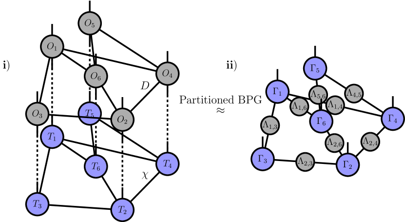
Figure 7: An example of BP gauging a partitioned network in the context of contracting a tensor network operator (TNO) composed of tensors $O_{v}$ with a tensor network state (TNS) composed of tensors $T_{v}$. i) - ii) The combined TNO-TNS network is partitioned, with the corresponding site tensors $O_{v}$ and $T_{v}$ grouped together. A generalized version of the belief propagation gauging routine is then performed on the partitioned structure and used to bring the state into the Vidal gauge and truncate the bonds of the resulting TNS to a desired dimension. The resulting state can then be transformed to the symmetric gauge via Eq. (27) and a new TNO can be applied. We emphasize that contracting the tensors within a partition does not need to be performed explicitly and for efficiency the two-layer network can be kept in memory while performing belief propagation on the norm network. This can lead to further efficiency improvements from BP gauging over eager and simple update gauging [132, 123] which effectively require pre-contracting the groups of tensors within partitions in the first iterations, leading to larger intermediate tensors in subsequent iterations of gauging.

.

3.5 Belief propagation gauging on a partitioned network: application to contracting tensor network operators with states

It is natural to consider a simple extension of belief propagation where the corresponding graphical model is first partitioned — i.e. local degrees of freedom are grouped together — and messages are defined between the different regions. This has previously been referred to as ‘block belief propagation’ [150] and is also related to the well-established generalized belief propagation method [154, 143, 144], although without the partitions overlapping.

In the context of gauging a tensor network state, partitioning can be used to generalize the belief propagation gauging procedure outlined in Fig. 3: a site tensor $T_{v}$ would be replaced by a group of tensors associated with the vertex group $v$. Then, each $\mathcal{T}_{v}$ would correspond to that associated group of tensors and their conjugates. Message tensors are then defined between the tensor groups $\mathcal{T}_{v}$ and iterated as usual. As is the case for generalized BP, the message tensors would generically grow exponentially with the size of the partitions, although this could be circumvented by approximating the message tensors themselves as tensor networks (such as MPSs [150]) and not just single tensors. The resulting message tensors can then be used to gauge the original network to obtain a $\Gamma_{v}$ site tensor associated with each vertex group $v$ and a $\Lambda_{e}$ bond tensor associated with each edge $e$ of the partitioned TNS, which then (approximately, up to BP convergence and possible truncations) obey the standard isometry conditions defined in Eqs. (1) and (2).

An application of BP gauging generalized to partitioned TNS is approximately contracting a tensor network operator (TNO) with a TNS, resulting in a new TNS, under the BP approximation. An example of this is illustrated in Fig. 7. TNOs arise naturally from long-range gates, layers of 3D classical partition functions and from grouping layers of gates together when performing gate evolution of a TNS. This latter application can be used as an alternative to evolving a TNS gate-by-gate and can provide higher accuracy since fewer truncations are performed. One can view the application of the TNO onto the TNS using the BP approximation as a two-layer network that is first partitioned by grouping each site tensor $T_{v}$ of the TNS with its corresponding site tensor $O_{v}$ of the TNO. BP gauging can then be used to regauge and truncate the resulting partitioned network, similar to previous work that used eager gauging [132] and simple update gauging [123] for the same task. In contrast with those methods, however, BP gauging does not require contracting the corresponding sites tensors of the TNO with the TNS ahead of time, since BP can be run on the partitioned network structure [154, 143, 150]. This can give further efficiency improvements from BP gauging compared to eager and simple update gauging beyond those we already demonstrated in Sec. 3.2 for gauging simple (un-partitioned) TNS. Those methods effectively require pre-contracting the groups of tensors within partitions in the first gauging iteration, leading to larger intermediate tensors in subsequent iterations of gauging. BP gauging of partitioned tensor networks was used in Ref. [189], where layers of gates of a 2D quantum circuit were represented as TNOs.

3.6 Gauging infinite tensor networks with belief propagation

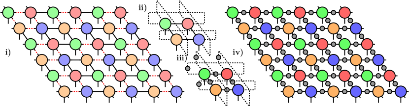
Figure 8: Gauging infinite tensor networks with BP gauging. i) Infinite 2D TNS (PEPS) with a $2\times 2$ unit cell. Unit cells are separated by red dotted lines. ii) Unit cell of the infinite 2D TNS but with additional periodic edges added (dashed lines). iii) Upon gauging the periodic unit cell new site tensors and bond tensors are determined which put it into the Vidal gauge. The bond tensors are not necessarily identical, and can be unique for each edge (in this example there are $8$). iv) The resulting site tensors and bond tensors from the periodic TNS determine the Vidal gauge for the infinite lattice. These tensors can be used to directly extract observables from the infinite TNS, for example via Eq. (36).

So far, we have mostly focused our attention on gauging finite tensor networks. Infinite tensor network states are, however, an important branch of research on tensor networks as they allow computations which work directly in the thermodynamic limit. There is extensive literature on gauging infinite tensor network states [119, 123, 132, 134].

Here we demonstrate how our belief propagation gauging routine can be used to gauge an infinite TNS and to compute observables under the BP approximation. Specifically, consider an infinite TNS which can be constructed by repeated translation of a finite tensor network. We can use belief propagation gauging to determine the corresponding bond and site tensors which transform the infinite TNS into the Vidal gauge. Specifically, one can take the tensor network state over the finite unit cell, add in appropriate periodic boundary conditions (in the form of additional bonds on the lattice), run BP on the periodic TNS and then use Eqs. (21), (22), and (23) to determine the corresponding bond tensors and site tensors which yield the periodic TNS in the Vidal gauge. It can be proven that these tensors are exactly those that transform the infinite TNS into the Vidal gauge. Fig. 8 illustrates gauging an infinite TNS for the square lattice with a $2\times 2$ unit cell — although we emphasize our method is independent of the network structure and can be easily applied to unstructured unit cells in arbitrary dimensions [114].

In order to demonstrate this procedure computationally, we consider the TNS corresponding to the square root of the Ising partition function on an infinite square lattice. The site tensors $T_{v}$ are all identical, with $z=4$, and their construction is described in Refs. [174, 149]. As a representation of the infinite TNS we take the same tensors as the finite case but on the vertices of a $3\times 3$ unit cell with periodic boundary conditions in both horizontal and vertical directions. We gauge this state with our belief propagation gauging routine and also gauge the same state but on a finite, open boundary $L\times L$ lattice.

In Fig. 9a, upon gauging the state, we approximately measure $\langle S^{z}_{v}\rangle$:

$$\leavevmode\hbox{$\vbox{\hbox{\resizebox{}{}{{\leavevmode\hbox{\set@color{}}}}}}$}\quad,$$ (36)

which essentially gives the best approximation for $\langle S^{z}_{v}\rangle$ under the assumption of a rank-one environment. It is equivalent to running belief propagation on the norm network of the periodic unit cell and measuring $\langle S^{z}_{v}\rangle$ using the fixed point message tensors:

$$\leavevmode\hbox{$\vbox{\hbox{\resizebox{}{}{{\leavevmode\hbox{\set@color{}}}}}}$}\quad.$$ (37)

The results in Fig. 9 show that the expectation value for $v$ in the middle of an increasingly large $L\times L$ open-boundary lattice converges to that of the small periodic unit cell. Using belief propagation to gauge the periodic TNS thus can be used to obtain results, under the approximation in Eq. (36), in $O(1)$ time in the lattice size for infinite networks (and $O(L)$ time where $L$ is the number of sites of the unit cell). This fact is implicitly used in the simple update gate evolution algorithm when applied to infinite PEPS.

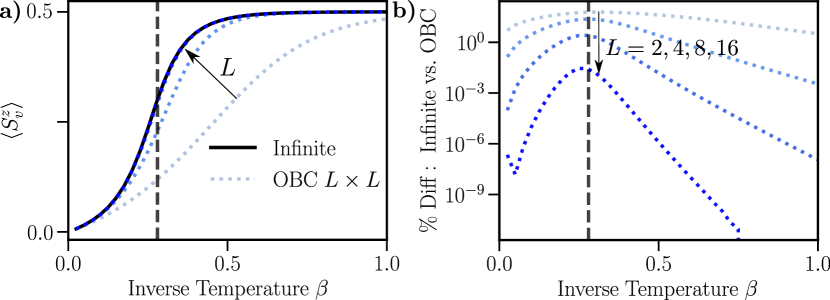
Figure 9: Gauging the tensor network state corresponding to the square root of the classical Ising partition function on a square lattice, with a longitudinal field of $h=0.5$. Black dashed line represents the point $\beta_{c}\approx 0.28$, which is the critical point under the Bethe approximation. a) Result from gauging the state and approximately measuring $\langle S^{z}_{v}\rangle$ using Eq. (36), taking $v$ to be the central site of the lattice. The solid black line shows the result from a $3\times 3$ periodic lattice (which is equivalent to an infinite lattice under the BP approximation — see text) while dotted lines show the result for an open boundary $L\times L$ lattice of increasing size ($L=2,4,8,$ and $16$) with the result converging to the infinite one. b) Percentage difference between the infinite and open boundary values of $\langle S^{z}_{v}\rangle$ for increasing open boundary lattice size ($L=2,4,8,$ and $16$).

4 Conclusion

In this work we have demonstrated how belief propagation (BP) can be used to bring an arbitrary tensor network state (TNS) into a gauge commonly used in the tensor network literature — which we refer to as the Vidal gauge but has previously been referred to as the super-orthogonal or quasi-canonical gauge — where multiple local orthogonality conditions are (approximately) satisfied. We showed that it can be viewed as a simplified version of a gauging method previously introduced in Refs. [132, 134]. We have benchmarked our ‘belief propagation gauging’ algorithm, demonstrating that it can be faster than existing algorithms for reaching the Vidal gauge. Additionally, we demonstrated the application of our new gauging algorithm to improving the accuracy of simple update gate evolution of TNS. We also discussed ‘block BP gauging’ which involves performing belief propagation gauging on a partition tensor network. We showed an example of block BP gauging in the context of the contraction of a TNS and a tensor network operator (TNO), and we argued that it has additional efficiency advantages in this context over currently available gauging methods because it can more effectively make use of a partitioned tensor network structure, which is utilized in the recent Ref. [189]. Finally, we demonstrated — by gauging small periodic systems — how to gauge infinite tensor network states with our algorithm and how this can be used to make approximate measurements corresponding to the thermodynamic limit.

Our new BP gauging method has a number of potential advantages over previous ones, in addition to the ones mentioned above. Because it is primarily based on BP, a well established method, optimized BP implementations as well as algorithmic advancements to BP (like the recent [151]) and generalizations of BP [154, 143, 150] can be repurposed for the application of gauging and truncating TNS. Additionally, the BP algorithm is very simple and is based only on tensor contractions (whereas previous gauging methods interspersed tensor contractions and factorizations). Therefore it is simpler to implement, optimize, and should be more straightforward to effectively make use of specialized hardware like GPUs or TPUs [190], where tensor contractions generally have bigger speedups than factorizations compared to CPUs. On a theoretical level, it would be interesting to investigate connections between various TNS gauging proposals (for example [125, 127, 133, 138, 131]) and explore if there is a more unified picture based on tensor contraction, in anology to the close connection that is now established between the belief propagation tensor network contraction algorithm and standard tensor network gauges.

5 Acknowledgements

5.1 Computing Resources and Software Packages

The code used to produce the numerical results in this paper was written using the ITensorNetworks.jl [170] package — a general purpose and publicly available Julia [191] package for manipulating (gauging, contracting, partitioning, evolving, truncating, optimizing, etc.) tensor network states of arbitrary geometry. It is built on top of ITensors.jl [192], which provides the basic tensor operations. Code is available in the current version of ITensorNetworks.jl for performing belief propagation gauging on arbitrary tensor network states. Code for using the other routines described in this paper is also available. An example is available which benchmarks these routines against each other. Our benchmarking was done using the Rusty cluster housed in the Flatiron Institute in New York, New York. All code was run using 10 cores of the same Skylake computing node.

The tensor network diagrams in this paper were produced using the publicly available package GraphTikz.jl [193], a general purpose Julia package for visualizing graphs, including tensor networks.

5.2 Funding and Discussions

J.T. and M.F. are grateful for ongoing support through the Flatiron Institute, a division of the Simons Foundation. We would like to thank Miles Stoudenmire for illuminating discussions. We would also like to thank Miles Stoudenmire, Johnnie Gray, and Nicola Pancotti for providing helpful comments on the manuscript.

Appendix A Simple update

Here we detail more efficient variants of the the simple update (SU) procedure — whose most direct implementation is shown in Fig. 5 — for applying a two-site gate $O_{v,w}$ to a TNS [119, 139, 122, 114]. The original TNS is taken to be in the Vidal form although we emphasize that the same efficiency improvements directly apply to the analogous BP variant of simple update (see Fig. 5b). Methods — such as the ‘reduced tensor’ method [122, 194, 96, 133, 113] — have been developed to improve the efficiency of the SU procedure by using orthogonal decompositions like the QR decomposition to apply the gate to a reduced space. In this work, when applying a gate to a TNS, we utilize this more efficient version of SU [194, 96]. We depict this version diagrammatically in Fig. 10.

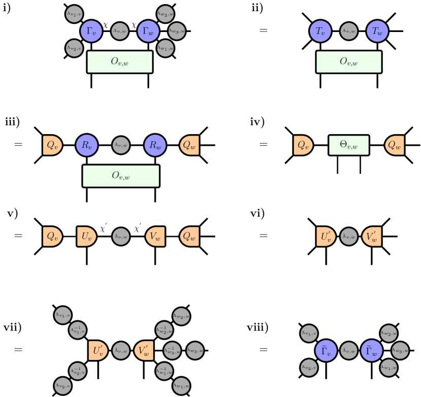
Figure 10: ‘Reduced tensor’ version of simple update described in Fig. 5. The example pictured shows a two-site gate $O_{v,w}$ being applied to neighbouring sites $v$ and $w$ with coordination numbers of $3$ and $4$ respectively. The dimension of the bond along the edge $e=(v,w)$ is $\chi$. i) - ii) The bond tensors are absorbed onto the site tensors. ii) - iii) A QR decomposition is performed on both the left and right site tensors. iii) - iv) The resulting $R_{v}$ and $R_{w}$ tensors, the bond tensor $\Lambda_{v,w}$, and the gate are combined together to form the composite tensor $\Theta_{v,w}$. iv) - v) The composite tensor is SVDd (with the bond being truncated down to dimension $\chi^{\prime}$) and the resulting singular values become the new bond tensor $\tilde{\Lambda}_{v,w}$. v) - vi) The $U_{v}$ and $V_{w}$ matrices from the SVD are multiplied back with $Q_{v}$ and $Q_{w}$. vi) - vii) Resolutions of identity using the previous bond tensors are inserted. vii) - viii) The inverses are absorbed to yield the updated bond tensors and site tensors. Such a procedure could be generalized to long-range gates by matrix product operator decompositions of the gate.

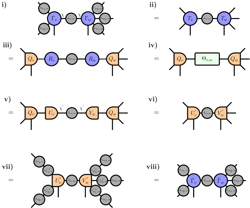
Figure 11: Simple update step when applying an identity matrix. This step is the workhorse of simple update gauging. The example pictured is two neighbouring sites with co-ordination numbers of $3$ and $4$ respectively. The bond dimension along the edge $e=(v,w)$ is $\chi$. i) - ii) The bond tensors are absorbed onto the site tensors. ii) - iii) A QR decomposition is performed on both the left and right site tensors. iii) - iv) The resulting $R$ tensors are combined together to form the composite $\Theta_{v,w}$. iv) - v) The composite tensor is SVDd (with the bond being truncated down to dimension $\chi^{\prime}\leq\chi$) and the resulting singular values become the new bond tensor $\tilde{\Lambda}_{v,w}$. v) - vi) The $U_{v}$ and $V_{w}$ matrices from the SVD are multiplied back with $Q_{v}$ and $Q_{w}$. vi) - vii) Resolutions of identity using the previous bond tensors are inserted. vii) - viii) The inverses are absorbed to yield the updated bond tensors and site tensors.

When performing simple update gauging, an identity gate is applied. This means the gate in Fig. 10 can be removed entirely and the physical, site indices can be moved onto the $Q$ tensors during the QR decomposition in order to improve efficiency [187]. This is the procedure we adopt when performing edge updates in the simple update gauging procedure (which is described in the following section). We illustrate this in Fig. 11.

Appendix B Gauging routines review

Here, we provide details of the existing gauging routines that we benchmark our ‘belief propagation gauging’ routine against in Fig. 4 of the main text.

The first, which we refer to as ‘simple update gauging’, involves repeated iterations of simple update (without any truncation) across the edges of a TNS with identity gates (see Fig. 11). This is known to bring the network closer to satisfying Eqs. (1) on every edge [123].

To be explicit, we implement the following routine to produce the results for ‘simple update gauging’ presented in Fig. 4 of the main text:

The simple update gauging routine

• Start with a TNS consisting of site tensors $\{\Gamma_{v}\}$ and bond tensors $\{\Lambda_{e}\}$. If the TNS is described only by site tensors (no bond tensors) then assign the bond tensors to identity matrices.

• Perform an iteration:

  • Iterate over each edge of the TNS and perform simple update with identity gates (i.e. the simple update variant shown in Fig. 11) to get new site tensors $\{\Gamma_{v}\}$ and bond tensors $\{\Lambda_{e}\}$.

• Repeatedly perform iterations until the designated stopping criteria is reached.

The second gauging routine we benchmark against we refer to as ‘eager gauging’, which was first introduced in Refs. [132, 134]. Specifically, the routine is equivalent to the following and was used to produce the results for ‘eager gauging’ presented in Fig. 4 of the main text:

The eager gauging routine

• Start with a TNS consisting of site tensors $\{T_{v}\}$. Form the closed, norm network of the TNS.

• Initialize the belief propagation message tensors of the norm network to arbitrary positive definite matrices — in our implementation we initialize them to identity matrices.

• Perform an iteration:

  • Do a single update of each message tensor via Eq. (5).

  • Gauge the TNS with the resulting message tensors via Eqs. (21), (22), and (23), yielding site tensors $\{\Gamma_{v}\}$ and bond tensors $\{\Lambda_{e}\}$.

  • Transform into the symmetric gauge by absorbing the square root bond tensors via Eq. (27), yielding a new set of site tensors $\{T_{v}\}$.

  • Assign the message tensors to the bond matrices found from gauging i.e. $M_{e}=M_{\bar{e}}=\Lambda_{e}$.

• Repeatedly perform iterations until the designated stopping criteria is reached, skipping the transformation into the symmetric gauge in the last iteration.

References

- [1] F. Verstraete, V. Murg and J.I. Cirac “Matrix product states, projected entangled pair states, and variational renormalization group methods for quantum spin systems” In Advances in Physics 57.2 Taylor & Francis, 2008, pp. 143–224 DOI: 10.1080/14789940801912366
- [2] Laurens Vanderstraeten, Jutho Haegeman and Frank Verstraete “Tangent-space methods for uniform matrix product states” In SciPost Physics Lecture Notes, 2019, pp. 007 DOI: 10.21468/SciPostPhysLectNotes.7
- [3] J. Cirac, David Perez-Garcia, Norbert Schuch and Frank Verstraete “Matrix product states and projected entangled pair states: Concepts, symmetries, theorems” In Rev. Mod. Phys. 93 American Physical Society, 2021, pp. 045003 DOI: 10.1103/RevModPhys.93.045003
- [4] “The Tensor Network: Resources for tensor network algorithms, theory, and software” In Tensor Network URL: https://tensornetwork.org
- [5] Glen Evenbly “Tensors.net: Resources for learning and implementing tensor network methods to study quantum many-body systems.” In Tensors.net URL: https://www.tensors.net
- [6] Ulrich Schollwöck “The density-matrix renormalization group in the age of matrix product states” January 2011 Special Issue In Annals of Physics 326.1, 2011, pp. 96–192 DOI: https://doi.org/10.1016/j.aop.2010.09.012
- [7] Román Orús “A practical introduction to tensor networks: Matrix product states and projected entangled pair states” arXiv:1306.2164 [cond-mat, physics:hep-lat, physics:hep-th, physics:quant-ph] In Annals of Physics 349, 2014, pp. 117–158 DOI: 10.1016/j.aop.2014.06.013
- [8] Andrzej Cichocki “Tensor Networks for Big Data Analytics and Large-Scale Optimization Problems” arXiv:1407.3124 [cs, math] type: article, 2014 DOI: 10.48550/arXiv.1407.3124
- [9] Andrzej Cichocki, Namgil Lee, Ivan Oseledets, Anh-Huy Phan, Qibin Zhao and Danilo P. Mandic “Tensor Networks for Dimensionality Reduction and Large-scale Optimization: Part 1 Low-Rank Tensor Decompositions” In Foundations and Trends® in Machine Learning 9.4-5 Now Publishers, Inc., 2016, pp. 249–429 DOI: 10.1561/2200000059
- [10] Jacob C. Bridgeman and Christopher T. Chubb “Hand-waving and interpretive dance: an introductory course on tensor networks” In Journal of Physics A: Mathematical and Theoretical 50.22 IOP Publishing, 2017, pp. 223001 DOI: 10.1088/1751-8121/aa6dc3
- [11] Jutho Haegeman and Frank Verstraete “Diagonalizing Transfer Matrices and Matrix Product Operators: A Medley of Exact and Computational Methods” In Annual Review of Condensed Matter Physics 8.1, 2017, pp. 355–406 DOI: 10.1146/annurev-conmatphys-031016-025507
- [12] Andrzej Cichocki, Anh-Huy Phan, Qibin Zhao, Namgil Lee, Ivan Oseledets, Masashi Sugiyama and Danilo P. Mandic “Tensor Networks for Dimensionality Reduction and Large-scale Optimization: Part 2 Applications and Future Perspectives” In Foundations and Trends® in Machine Learning 9.6 Now Publishers, Inc., 2017, pp. 431–673 DOI: 10.1561/2200000067
- [13] Román Orús “Tensor networks for complex quantum systems” arXiv:1812.04011 [cond-mat, physics:hep-lat, physics:quant-ph] In Nature Reviews Physics 1.9 Nature Publishing Group, 2019, pp. 538–550 DOI: 10.1038/s42254-019-0086-7
- [14] Simeng Yan, David A. Huse and Steven R. White “Spin-Liquid Ground State of the Kagome Heisenberg Antiferromagnet” In Science 332.6034, 2011, pp. 1173–1176 DOI: 10.1126/science.1201080
- [15] Stefan Depenbrock, Ian P. McCulloch and Ulrich Schollwöck “Nature of the Spin-Liquid Ground State of the Heisenberg Model on the Kagome Lattice” In Physical Review Letters 109.6 American Physical Society, 2012, pp. 067201 DOI: 10.1103/PhysRevLett.109.067201
- [16] F. Kolley, S. Depenbrock, I.. McCulloch, U. Schollwöck and V. Alba “Phase diagram of the Heisenberg model on the kagome lattice” In Physical Review B 91.10 American Physical Society, 2015, pp. 104418 DOI: 10.1103/PhysRevB.91.104418
- [17] Simons Collaboration on the Many-Electron Problem et al. “Solutions of the Two-Dimensional Hubbard Model: Benchmarks and Results from a Wide Range of Numerical Algorithms” In Physical Review X 5.4 American Physical Society, 2015, pp. 041041 DOI: 10.1103/PhysRevX.5.041041
- [18] Yin-Chen He, Michael P. Zaletel, Masaki Oshikawa and Frank Pollmann “Signatures of Dirac Cones in a DMRG Study of the Kagome Heisenberg Model” In Physical Review X 7.3 American Physical Society, 2017, pp. 031020 DOI: 10.1103/PhysRevX.7.031020
- [19] Bo-Xiao Zheng et al. “Stripe order in the underdoped region of the two-dimensional Hubbard model” In Science 358.6367, 2017, pp. 1155–1160 DOI: 10.1126/science.aam7127
- [20] Simons Collaboration on the Many-Electron Problem, Mingpu Qin, Chia-Min Chung, Hao Shi, Ettore Vitali, Claudius Hubig, Ulrich Schollwöck, Steven R. White and Shiwei Zhang “Absence of Superconductivity in the Pure Two-Dimensional Hubbard Model” In Physical Review X 10.3 American Physical Society, 2020, pp. 031016 DOI: 10.1103/PhysRevX.10.031016
- [21] Hao Xu, Chia-Min Chung, Mingpu Qin, Ulrich Schollwöck, Steven R. White and Shiwei Zhang “Coexistence of superconductivity with partially filled stripes in the Hubbard model” arXiv:2303.08376 [cond-mat, physics:physics] type: article, 2023 DOI: 10.48550/arXiv.2303.08376
- [22] Steven R. White and Richard L. Martin “Ab initio quantum chemistry using the density matrix renormalization group” In The Journal of Chemical Physics 110.9 American Institute of Physics, 1999, pp. 4127–4130 DOI: 10.1063/1.478295
- [23] Alberto Baiardi and Markus Reiher “The density matrix renormalization group in chemistry and molecular physics: Recent developments and new challenges” In The Journal of Chemical Physics 152.4 American Institute of Physics, 2020, pp. 040903 DOI: 10.1063/1.5129672
- [24] Garnet Kin-Lic Chan and Sandeep Sharma “The Density Matrix Renormalization Group in Quantum Chemistry” In Annual Review of Physical Chemistry 62.1, 2011, pp. 465–481 DOI: 10.1146/annurev-physchem-032210-103338
- [25] Naoki Nakatani and Garnet Kin-Lic Chan “Efficient tree tensor network states (TTNS) for quantum chemistry: Generalizations of the density matrix renormalization group algorithm” In The Journal of Chemical Physics 138.13 American Institute of Physics, 2013, pp. 134113 DOI: 10.1063/1.4798639
- [26] Yuki Kurashige, Garnet Kin-Lic Chan and Takeshi Yanai “Entangled quantum electronic wavefunctions of the Mn4CaO5 cluster in photosystem II” In Nature Chemistry 5.8 Nature Publishing Group, 2013, pp. 660–666 DOI: 10.1038/nchem.1677
- [27] Szilárd Szalay, Max Pfeffer, Valentin Murg, Gergely Barcza, Frank Verstraete, Reinhold Schneider and Örs Legeza “Tensor product methods and entanglement optimization for ab initio quantum chemistry” arXiv:1412.5829 [cond-mat, physics:math-ph, physics:physics, physics:quant-ph] In International Journal of Quantum Chemistry 115.19, 2015, pp. 1342–1391 DOI: 10.1002/qua.24898
- [28] Yiqing Zhou, E. Stoudenmire and Xavier Waintal “What Limits the Simulation of Quantum Computers?” In Physical Review X 10.4 American Physical Society, 2020, pp. 041038 DOI: 10.1103/PhysRevX.10.041038
- [29] Johnnie Gray and Stefanos Kourtis “Hyper-optimized tensor network contraction” In Quantum 5 Verein zur Förderung des Open Access Publizierens in den Quantenwissenschaften, 2021, pp. 410 DOI: 10.22331/q-2021-03-15-410
- [30] Jielun Chen, E.. Stoudenmire and Steven R. White “The Quantum Fourier Transform Has Small Entanglement” arXiv:2210.08468 [quant-ph] type: article, 2022 DOI: 10.48550/arXiv.2210.08468
- [31] Feng Pan and Pan Zhang “Simulation of Quantum Circuits Using the Big-Batch Tensor Network Method” In Physical Review Letters 128.3 American Physical Society, 2022, pp. 030501 DOI: 10.1103/PhysRevLett.128.030501
- [32] Feng Pan, Keyang Chen and Pan Zhang “Solving the Sampling Problem of the Sycamore Quantum Circuits” In Physical Review Letters 129.9 American Physical Society, 2022, pp. 090502 DOI: 10.1103/PhysRevLett.129.090502
- [33] Thomas Ayral, Thibaud Louvet, Yiqing Zhou, Cyprien Lambert, E. Stoudenmire and Xavier Waintal “Density-Matrix Renormalization Group Algorithm for Simulating Quantum Circuits with a Finite Fidelity” In PRX Quantum 4.2 American Physical Society, 2023, pp. 020304 DOI: 10.1103/PRXQuantum.4.020304
- [34] Joseph Tindall, Matt Fishman, Miles Stoudenmire and Dries Sels “Efficient tensor network simulation of IBM’s kicked Ising experiment”, 2023 arXiv:2306.14887 [quant-ph]
- [35] Edwin Stoudenmire and David J Schwab “Supervised Learning with Tensor Networks” In Advances in Neural Information Processing Systems 29 Curran Associates, Inc., 2016 URL: https://papers.nips.cc/paper_files/paper/2016/hash/5314b9674c86e3f9d1ba25ef9bb32895-Abstract.html
- [36] Zhao-Yu Han, Jun Wang, Heng Fan, Lei Wang and Pan Zhang “Unsupervised Generative Modeling Using Matrix Product States” In Physical Review X 8.3 American Physical Society, 2018, pp. 031012 DOI: 10.1103/PhysRevX.8.031012
- [37] Ding Liu, Shi-Ju Ran, Peter Wittek, Cheng Peng, Raul Blázquez García, Gang Su and Maciej Lewenstein “Machine learning by unitary tensor network of hierarchical tree structure” In New Journal of Physics 21.7 IOP Publishing, 2019, pp. 073059 DOI: 10.1088/1367-2630/ab31ef
- [38] William Huggins, Piyush Patil, Bradley Mitchell, K. Whaley and E. Stoudenmire “Towards quantum machine learning with tensor networks” In Quantum Science and Technology 4.2 IOP Publishing, 2019, pp. 024001 DOI: 10.1088/2058-9565/aaea94
- [39] I.. Oseledets “Approximation of Matrices Using Tensor Decomposition” In SIAM Journal on Matrix Analysis and Applications 31.4, 2010, pp. 2130–2145 DOI: 10.1137/090757861
- [40] Boris N. Khoromskij “O(dlog N)-Quantics Approximation of N-d Tensors in High-Dimensional Numerical Modeling” In Constructive Approximation 34.2, 2011, pp. 257–280 DOI: 10.1007/s00365-011-9131-1
- [41] S.. Dolgov, B.. Khoromskij and I.. Oseledets “Fast Solution of Parabolic Problems in the Tensor Train/Quantized Tensor Train Format with Initial Application to the Fokker–Planck Equation” In SIAM Journal on Scientific Computing 34.6 Society for IndustrialApplied Mathematics, 2012, pp. A3016–A3038 DOI: 10.1137/120864210
- [42] Boris N. Khoromskij “Tensor Numerical Methods for High-dimensional PDEs: Basic Theory and Initial Applications” arXiv:1408.4053 [math] type: article, 2014 DOI: 10.48550/arXiv.1408.4053
- [43] Michael Lubasch, Pierre Moinier and Dieter Jaksch “Multigrid renormalization” In Journal of Computational Physics 372, 2018, pp. 587–602 DOI: 10.1016/j.jcp.2018.06.065
- [44] Juan José García-Ripoll “Quantum-inspired algorithms for multivariate analysis: from interpolation to partial differential equations” In Quantum 5 Verein zur Förderung des Open Access Publizierens in den Quantenwissenschaften, 2021, pp. 431 DOI: 10.22331/q-2021-04-15-431
- [45] Lorenz Richter, Leon Sallandt and Nikolas Nüsken “Solving high-dimensional parabolic PDEs using the tensor train format” PMLR, 2021, pp. 8998–9009 URL: https://proceedings.mlr.press/v139/richter21a.html
- [46] Nikita Gourianov, Michael Lubasch, Sergey Dolgov, Quincy Y. Berg, Hessam Babaee, Peyman Givi, Martin Kiffner and Dieter Jaksch “A quantum-inspired approach to exploit turbulence structures” In Nature Computational Science 2.1 Nature Publishing Group, 2022, pp. 30–37 DOI: 10.1038/s43588-021-00181-1
- [47] Nikita Gourianov “Exploiting the structure of turbulence with tensor networks” University of Oxford, 2022 URL: https://ora.ox.ac.uk/objects/uuid:9e3f4786-ad68-4913-9a0d-e9b1e108128f
- [48] Jacob D. Biamonte, Jason Morton and Jacob Turner “Tensor Network Contractions for #SAT” In Journal of Statistical Physics 160.5, 2015, pp. 1389–1404 DOI: 10.1007/s10955-015-1276-z
- [49] Stefanos Kourtis, Claudio Chamon, Eduardo Mucciolo and Andrei Ruckenstein “Fast counting with tensor networks” In SciPost Physics 7.5, 2019, pp. 060 DOI: 10.21468/SciPostPhys.7.5.060
- [50] Samuel Mugel, Carlos Kuchkovsky, Escolástico Sánchez, Samuel Fernández-Lorenzo, Jorge Luis-Hita, Enrique Lizaso and Román Orús “Dynamic portfolio optimization with real datasets using quantum processors and quantum-inspired tensor networks” In Physical Review Research 4.1 American Physical Society, 2022, pp. 013006 DOI: 10.1103/PhysRevResearch.4.013006
- [51] Raj G. Patel et al. “Application of Tensor Neural Networks to Pricing Bermudan Swaptions” arXiv:2304.09750 [quant-ph, q-fin] type: article, 2023 DOI: 10.48550/arXiv.2304.09750
- [52] Steven R. White “Density matrix formulation for quantum renormalization groups” In Physical Review Letters 69.19 American Physical Society, 1992, pp. 2863–2866 DOI: 10.1103/PhysRevLett.69.2863
- [53] Sebastian Holtz, Thorsten Rohwedder and Reinhold Schneider “The Alternating Linear Scheme for Tensor Optimization in the Tensor Train Format” In SIAM Journal on Scientific Computing 34.2 Society for IndustrialApplied Mathematics, 2012, pp. A683–A713 DOI: 10.1137/100818893
- [54] I.. Oseledets and S.. Dolgov “Solution of Linear Systems and Matrix Inversion in the TT-Format” In SIAM Journal on Scientific Computing 34.5, 2012, pp. A2718–A2739 DOI: 10.1137/110833142
- [55] S.. Dolgov “TT-GMRES: solution to a linear system in the structured tensor format” In Russian Journal of Numerical Analysis and Mathematical Modelling 28.2 De Gruyter, 2013, pp. 149–172 DOI: 10.1515/rnam-2013-0009
- [56] Sergey V. Dolgov and Dmitry V. Savostyanov “Alternating Minimal Energy Methods for Linear Systems in Higher Dimensions” In SIAM Journal on Scientific Computing 36.5 Society for IndustrialApplied Mathematics, 2014, pp. A2248–A2271 DOI: 10.1137/140953289
- [57] Sergey V. Dolgov and Dmitry V. Savostyanov “Corrected One-Site Density Matrix Renormalization Group and Alternating Minimal Energy Algorithm” In Numerical Mathematics and Advanced Applications - ENUMATH 2013, Lecture Notes in Computational Science and Engineering Cham: Springer International Publishing, 2015, pp. 335–343 DOI: 10.1007/978-3-319-10705-9_33
- [58] Christian Lubich, Ivan V. Oseledets and Bart Vandereycken “Time Integration of Tensor Trains” In SIAM Journal on Numerical Analysis 53.2, 2015, pp. 917–941 DOI: 10.1137/140976546
- [59] C. Hubig, I.. McCulloch, U. Schollwöck and F.. Wolf “Strictly single-site DMRG algorithm with subspace expansion” In Physical Review B 91.15 American Physical Society, 2015, pp. 155115 DOI: 10.1103/PhysRevB.91.155115
- [60] Vedika Khemani, Frank Pollmann and S.. Sondhi “Obtaining Highly Excited Eigenstates of Many-Body Localized Hamiltonians by the Density Matrix Renormalization Group Approach” In Phys. Rev. Lett. 116 American Physical Society, 2016, pp. 247204 DOI: 10.1103/PhysRevLett.116.247204
- [61] Steven R. White “Density-matrix algorithms for quantum renormalization groups” In Physical Review B 48.14 American Physical Society, 1993, pp. 10345–10356 DOI: 10.1103/PhysRevB.48.10345
- [62] Jutho Haegeman, Christian Lubich, Ivan Oseledets, Bart Vandereycken and Frank Verstraete “Unifying time evolution and optimization with matrix product states” In Physical Review B 94.16 American Physical Society, 2016, pp. 165116 DOI: 10.1103/PhysRevB.94.165116
- [63] Brenden Roberts, Thomas Vidick and Olexei I. Motrunich “Implementation of rigorous renormalization group method for ground space and low-energy states of local Hamiltonians” In Phys. Rev. B 96 American Physical Society, 2017, pp. 214203 DOI: 10.1103/PhysRevB.96.214203
- [64] Sergey V. Dolgov “A Tensor Decomposition Algorithm for Large ODEs with Conservation Laws” In Computational Methods in Applied Mathematics 19.1 De Gruyter, 2019, pp. 23–38 DOI: 10.1515/cmam-2018-0023
- [65] Eric Jeckelmann “Dynamical density-matrix renormalization-group method” In Physical Review B 66.4 American Physical Society, 2002, pp. 045114 DOI: 10.1103/PhysRevB.66.045114
- [66] Guifré Vidal “Efficient Classical Simulation of Slightly Entangled Quantum Computations” In Physical Review Letters 91.14 American Physical Society, 2003, pp. 147902 DOI: 10.1103/PhysRevLett.91.147902
- [67] Guifré Vidal “Efficient Simulation of One-Dimensional Quantum Many-Body Systems” In Physical Review Letters 93.4 American Physical Society, 2004, pp. 040502 DOI: 10.1103/PhysRevLett.93.040502
- [68] Steven R. White “Density matrix renormalization group algorithms with a single center site” In Physical Review B 72.18 American Physical Society, 2005, pp. 180403 DOI: 10.1103/PhysRevB.72.180403
- [69] Ian P McCulloch “From density-matrix renormalization group to matrix product states” In Journal of Statistical Mechanics: Theory and Experiment 2007.10, 2007, pp. P10014 DOI: 10.1088/1742-5468/2007/10/P10014
- [70] Jutho Haegeman, J. Cirac, Tobias J. Osborne, Iztok Pi žorn, Henri Verschelde and Frank Verstraete “Time-Dependent Variational Principle for Quantum Lattices” In Phys. Rev. Lett. 107 American Physical Society, 2011, pp. 070601 DOI: 10.1103/PhysRevLett.107.070601
- [71] I.. Oseledets “Tensor-Train Decomposition” In SIAM Journal on Scientific Computing 33.5 Society for IndustrialApplied Mathematics, 2011, pp. 2295–2317 DOI: 10.1137/090752286
- [72] Stellan Östlund and Stefan Rommer “Thermodynamic Limit of Density Matrix Renormalization” In Physical Review Letters 75.19 American Physical Society, 1995, pp. 3537–3540 DOI: 10.1103/PhysRevLett.75.3537
- [73] Stefan Rommer and Stellan Östlund “Class of ansatz wave functions for one-dimensional spin systems and their relation to the density matrix renormalization group” In Physical Review B 55.4 American Physical Society, 1997, pp. 2164–2181 DOI: 10.1103/PhysRevB.55.2164
- [74] G. Vidal “Classical Simulation of Infinite-Size Quantum Lattice Systems in One Spatial Dimension” In Physical Review Letters 98.7 American Physical Society, 2007, pp. 070201 DOI: 10.1103/PhysRevLett.98.070201
- [75] R. Orús and G. Vidal “Infinite time-evolving block decimation algorithm beyond unitary evolution” In Physical Review B 78.15 American Physical Society, 2008, pp. 155117 DOI: 10.1103/PhysRevB.78.155117
- [76] I.. McCulloch “Infinite size density matrix renormalization group, revisited” arXiv:0804.2509 [cond-mat] type: article, 2008 DOI: 10.48550/arXiv.0804.2509
- [77] V. Zauner, D. Draxler, L. Vanderstraeten, M. Degroote, J. Haegeman, M.. Rams, V. Stojevic, N. Schuch and F. Verstraete “Transfer matrices and excitations with matrix product states” In New Journal of Physics 17.5 IOP Publishing, 2015, pp. 053002 DOI: 10.1088/1367-2630/17/5/053002
- [78] V. Zauner-Stauber, L. Vanderstraeten, M.. Fishman, F. Verstraete and J. Haegeman “Variational optimization algorithms for uniform matrix product states” In Physical Review B 97.4 American Physical Society, 2018, pp. 045145 DOI: 10.1103/PhysRevB.97.045145
- [79] Y.-Y. Shi, L.-M. Duan and G. Vidal “Classical simulation of quantum many-body systems with a tree tensor network” In Physical Review A 74.2 American Physical Society, 2006, pp. 022320 DOI: 10.1103/PhysRevA.74.022320
- [80] Daniel Bauernfeind and Markus Aichhorn “Time dependent variational principle for tree Tensor Networks” In SciPost Physics 8.2, 2020, pp. 024 DOI: 10.21468/SciPostPhys.8.2.024
- [81] Benedikt Kloss, David Reichman and Yevgeny Bar Lev “Studying dynamics in two-dimensional quantum lattices using tree tensor network states” In SciPost Physics 9.5, 2020, pp. 070 DOI: 10.21468/SciPostPhys.9.5.070
- [82] Gianluca Ceruti, Christian Lubich and Hanna Walach “Time Integration of Tree Tensor Networks” In SIAM Journal on Numerical Analysis 59.1 Society for IndustrialApplied Mathematics, 2021, pp. 289–313 DOI: 10.1137/20M1321838
- [83] Philipp Seitz, Ismael Medina, Esther Cruz, Qunsheng Huang and Christian B. Mendl “Simulating quantum circuits using tree tensor networks” In Quantum 7 Verein zur Förderung des Open Access Publizierens in den Quantenwissenschaften, 2023, pp. 964 DOI: 10.22331/q-2023-03-30-964
- [84] W. Hackbusch and S. Kühn “A New Scheme for the Tensor Representation” In Journal of Fourier Analysis and Applications 15.5, 2009, pp. 706–722 DOI: 10.1007/s00041-009-9094-9
- [85] L. Tagliacozzo, G. Evenbly and G. Vidal “Simulation of two-dimensional quantum systems using a tree tensor network that exploits the entropic area law” In Physical Review B 80.23 American Physical Society, 2009, pp. 235127 DOI: 10.1103/PhysRevB.80.235127
- [86] Lars Grasedyck “Hierarchical Singular Value Decomposition of Tensors” In SIAM Journal on Matrix Analysis and Applications 31.4 Society for IndustrialApplied Mathematics, 2010, pp. 2029–2054 DOI: 10.1137/090764189
- [87] Christian Lubich, Thorsten Rohwedder, Reinhold Schneider and Bart Vandereycken “Dynamical Approximation by Hierarchical Tucker and Tensor-Train Tensors” In SIAM Journal on Matrix Analysis and Applications 34.2 Society for IndustrialApplied Mathematics, 2013, pp. 470–494 DOI: 10.1137/120885723
- [88] Daniel Bauernfeind, Manuel Zingl, Robert Triebl, Markus Aichhorn and Hans Gerd Evertz “Fork Tensor-Product States: Efficient Multiorbital Real-Time DMFT Solver” In Physical Review X 7.3 American Physical Society, 2017, pp. 031013 DOI: 10.1103/PhysRevX.7.031013
- [89] Klaas Gunst, Frank Verstraete, Sebastian Wouters, Örs Legeza and Dimitri Van Neck “T3NS: Three-Legged Tree Tensor Network States” In Journal of Chemical Theory and Computation 14.4 American Chemical Society, 2018, pp. 2026–2033 DOI: 10.1021/acs.jctc.8b00098
- [90] Natalia Chepiga and Steven R. White “Comb tensor networks” In Physical Review B 99.23 American Physical Society, 2019, pp. 235426 DOI: 10.1103/PhysRevB.99.235426
- [91] Hiromi Otsuka “Density-matrix renormalization-group study of the spin- XXZ antiferromagnet on the Bethe lattice” In Physical Review B 53.21 American Physical Society, 1996, pp. 14004–14007 DOI: 10.1103/PhysRevB.53.14004
- [92] Barry Friedman “A density matrix renormalization group approach to interacting quantum systems on Cayley trees” In Journal of Physics: Condensed Matter 9.42, 1997, pp. 9021 DOI: 10.1088/0953-8984/9/42/016
- [93] M.-B. Lepetit, M. Cousy and G.M. Pastor “Density-matrix renormalization study of the Hubbard model [4]on a Bethe lattice” In The European Physical Journal B - Condensed Matter and Complex Systems 13.3, 2000, pp. 421–427 DOI: 10.1007/s100510050053
- [94] Daniel Nagaj, Edward Farhi, Jeffrey Goldstone, Peter Shor and Igor Sylvester “Quantum transverse-field Ising model on an infinite tree from matrix product states” In Physical Review B 77.21 American Physical Society, 2008, pp. 214431 DOI: 10.1103/PhysRevB.77.214431
- [95] Manoranjan Kumar, S. Ramasesha and Zoltán G. Soos “Density matrix renormalization group algorithm for Bethe lattices of spin- or spin-1 sites with Heisenberg antiferromagnetic exchange” In Physical Review B 85.13 American Physical Society, 2012, pp. 134415 DOI: 10.1103/PhysRevB.85.134415
- [96] Wei Li, Jan Delft and Tao Xiang “Efficient simulation of infinite tree tensor network states on the Bethe lattice” In Physical Review B 86.19 American Physical Society, 2012, pp. 195137 DOI: 10.1103/PhysRevB.86.195137
- [97] Ádám Nagy “Simulating quantum systems on the Bethe lattice by translationally invariant infinite-tree tensor network” In Annals of Physics 327.2, 2012, pp. 542–552 DOI: 10.1016/j.aop.2011.11.012
- [98] Stefan Depenbrock and Frank Pollmann “Phase diagram of the isotropic spin- model on the Bethe lattice” In Physical Review B 88.3 American Physical Society, 2013, pp. 035138 DOI: 10.1103/PhysRevB.88.035138
- [99] Peter Lunts, Antoine Georges, E. Stoudenmire and Matthew Fishman “Hubbard model on the Bethe lattice via variational uniform tree states: Metal-insulator transition and a Fermi liquid” In Physical Review Research 3.2 American Physical Society, 2021, pp. 023054 DOI: 10.1103/PhysRevResearch.3.023054
- [100] Jianyu Xu, Ling Liang, Lei Deng, Changyun Wen, Yuan Xie and Guoqi Li “Towards a polynomial algorithm for optimal contraction sequence of tensor networks from trees” In Phys. Rev. E 100 American Physical Society, 2019, pp. 043309 DOI: 10.1103/PhysRevE.100.043309
- [101] Mihail Stoian “On the Optimal Linear Contraction Order for Tree Tensor Networks”, 2023 arXiv:2209.12332 [quant-ph]
- [102] D. Perez-Garcia, F. Verstraete, M.. Wolf and J.. Cirac “Matrix product state representations” In Quantum Information & Computation 7.5, 2007, pp. 401–430
- [103] Jutho Haegeman, Tobias J. Osborne and Frank Verstraete “Post-matrix product state methods: To tangent space and beyond” In Phys. Rev. B 88 American Physical Society, 2013, pp. 075133 DOI: 10.1103/PhysRevB.88.075133
- [104] Jutho Haegeman, Michaël Mariën, Tobias J. Osborne and Frank Verstraete “Geometry of matrix product states: Metric, parallel transport, and curvature” 021902 In Journal of Mathematical Physics 55.2, 2014 DOI: 10.1063/1.4862851
- [105] C. Hubig, J. Haegeman and U. Schollwöck “Error estimates for extrapolations with matrix-product states” In Physical Review B 97.4 American Physical Society, 2018, pp. 045125 DOI: 10.1103/PhysRevB.97.045125
- [106] Andreas Gleis, Jheng-Wei Li and Jan Delft “Projector formalism for kept and discarded spaces of matrix product states” In Physical Review B 106.19 American Physical Society, 2022, pp. 195138 DOI: 10.1103/PhysRevB.106.195138
- [107] André Uschmajew and Bart Vandereycken “The geometry of algorithms using hierarchical tensors” In Linear Algebra and its Applications 439.1, 2013, pp. 133–166 DOI: 10.1016/j.laa.2013.03.016
- [108] F. Verstraete, D. Porras and J.. Cirac “Density Matrix Renormalization Group and Periodic Boundary Conditions: A Quantum Information Perspective” In Physical Review Letters 93.22 American Physical Society, 2004, pp. 227205 DOI: 10.1103/PhysRevLett.93.227205
- [109] Peter Pippan, Steven R. White and Hans Gerd Evertz “Efficient matrix-product state method for periodic boundary conditions” In Physical Review B 81.8 American Physical Society, 2010, pp. 081103 DOI: 10.1103/PhysRevB.81.081103
- [110] Qibin Zhao, Guoxu Zhou, Shengli Xie, Liqing Zhang and Andrzej Cichocki “Tensor Ring Decomposition” arXiv:1606.05535 [cs] type: article, 2016 DOI: 10.48550/arXiv.1606.05535
- [111] Oscar Mickelin and Sertac Karaman “On algorithms for and computing with the tensor ring decomposition” In Numerical Linear Algebra with Applications 27.3, 2020, pp. e2289 DOI: 10.1002/nla.2289
- [112] Tomotoshi Nishino, Yasuhiro Hieida, Kouichi Okunishi, Nobuya Maeshima, Yasuhiro Akutsu and Andrej Gendiar “Two-Dimensional Tensor Product Variational Formulation” In Progress of Theoretical Physics 105.3, 2001, pp. 409–417 DOI: 10.1143/PTP.105.409
- [113] Ho N. Phien, Johann A. Bengua, Hoang D. Tuan, Philippe Corboz and Román Orús “Infinite projected entangled pair states algorithm improved: Fast full update and gauge fixing” In Physical Review B 92.3 American Physical Society, 2015, pp. 035142 DOI: 10.1103/PhysRevB.92.035142
- [114] Saeed S. Jahromi and Román Orús “Universal tensor-network algorithm for any infinite lattice” In Physical Review B 99.19 American Physical Society, 2019, pp. 195105 DOI: 10.1103/PhysRevB.99.195105
- [115] Patrick C.. Vlaar and Philippe Corboz “Simulation of three-dimensional quantum systems with projected entangled-pair states” In Physical Review B 103.20 American Physical Society, 2021, pp. 205137 DOI: 10.1103/PhysRevB.103.205137
- [116] Nobuya Maeshima, Yasuhiro Hieida, Yasuhiro Akutsu, Tomotoshi Nishino and Kouichi Okunishi “Vertical density matrix algorithm: A higher-dimensional numerical renormalization scheme based on the tensor product state ansatz” In Physical Review E 64.1 American Physical Society, 2001, pp. 016705 DOI: 10.1103/PhysRevE.64.016705
- [117] F. Verstraete and J.. Cirac “Renormalization algorithms for Quantum-Many Body Systems in two and higher dimensions” arXiv:cond-mat/0407066 type: article, 2004 DOI: 10.48550/arXiv.cond-mat/0407066
- [118] Y. Nishio, N. Maeshima, A. Gendiar and T. Nishino “Tensor Product Variational Formulation for Quantum Systems” arXiv:cond-mat/0401115 type: article, 2004 DOI: 10.48550/arXiv.cond-mat/0401115
- [119] H.. Jiang, Z.. Weng and T. Xiang “Accurate Determination of Tensor Network State of Quantum Lattice Models in Two Dimensions” In Physical Review Letters 101.9 American Physical Society, 2008, pp. 090603 DOI: 10.1103/PhysRevLett.101.090603
- [120] J. Jordan, R. Orús, G. Vidal, F. Verstraete and J.. Cirac “Classical Simulation of Infinite-Size Quantum Lattice Systems in Two Spatial Dimensions” In Physical Review Letters 101.25 American Physical Society, 2008, pp. 250602 DOI: 10.1103/PhysRevLett.101.250602
- [121] Román Orús and Guifré Vidal “Simulation of two-dimensional quantum systems on an infinite lattice revisited: Corner transfer matrix for tensor contraction” In Physical Review B 80.9 American Physical Society, 2009, pp. 094403 DOI: 10.1103/PhysRevB.80.094403
- [122] Philippe Corboz, Román Orús, Bela Bauer and Guifré Vidal “Simulation of strongly correlated fermions in two spatial dimensions with fermionic projected entangled-pair states” In Physical Review B 81.16 American Physical Society, 2010, pp. 165104 DOI: 10.1103/PhysRevB.81.165104
- [123] Henning Kalis, Daniel Klagges, Román Orús and Kai Phillip Schmidt “Fate of the cluster state on the square lattice in a magnetic field” In Physical Review A 86.2 American Physical Society, 2012, pp. 022317 DOI: 10.1103/PhysRevA.86.022317
- [124] Norbert Schuch, Michael M. Wolf, Frank Verstraete and J. Cirac “Computational Complexity of Projected Entangled Pair States” In Phys. Rev. Lett. 98 American Physical Society, 2007, pp. 140506 DOI: 10.1103/PhysRevLett.98.140506
- [125] Reza Haghshenas, Matthew J. O’Rourke and Garnet Kin-Lic Chan “Conversion of projected entangled pair states into a canonical form” In Physical Review B 100.5 American Physical Society, 2019, pp. 054404 DOI: 10.1103/PhysRevB.100.054404
- [126] Tomohiro Soejima, Karthik Siva, Nick Bultinck, Shubhayu Chatterjee, Frank Pollmann and Michael P. Zaletel “Isometric tensor network representation of string-net liquids” In Physical Review B 101.8 American Physical Society, 2020, pp. 085117 DOI: 10.1103/PhysRevB.101.085117
- [127] Michael P. Zaletel and Frank Pollmann “Isometric Tensor Network States in Two Dimensions” In Physical Review Letters 124.3 American Physical Society, 2020, pp. 037201 DOI: 10.1103/PhysRevLett.124.037201
- [128] Katharine Hyatt and E.. Stoudenmire “DMRG Approach to Optimizing Two-Dimensional Tensor Networks”, 2020 arXiv:1908.08833 [cond-mat.str-el]
- [129] Maurits S.. Tepaske and David J. Luitz “Three-dimensional isometric tensor networks” In Physical Review Research 3.2 American Physical Society, 2021, pp. 023236 DOI: 10.1103/PhysRevResearch.3.023236
- [130] Sheng-Hsuan Lin, Michael P. Zaletel and Frank Pollmann “Efficient simulation of dynamics in two-dimensional quantum spin systems with isometric tensor networks” In Physical Review B 106.24 American Physical Society, 2022, pp. 245102 DOI: 10.1103/PhysRevB.106.245102
- [131] Arturo Acuaviva, Visu Makam, Harold Nieuwboer, David Pérez-García, Friedrich Sittner, Michael Walter and Freek Witteveen “The minimal canonical form of a tensor network”, 2022 arXiv:2209.14358 [quant-ph]
- [132] Shi-Ju Ran, Wei Li, Bin Xi, Zhe Zhang and Gang Su “Optimized decimation of tensor networks with super-orthogonalization for two-dimensional quantum lattice models” In Physical Review B 86.13 American Physical Society, 2012, pp. 134429 DOI: 10.1103/PhysRevB.86.134429
- [133] Michael Lubasch, J. Cirac and Mari-Carmen Bañuls “Algorithms for finite projected entangled pair states” In Physical Review B 90.6 American Physical Society, 2014, pp. 064425 DOI: 10.1103/PhysRevB.90.064425
- [134] Ho N. Phien, Ian P. McCulloch and Guifré Vidal “Fast convergence of imaginary time evolution tensor network algorithms by recycling the environment” In Physical Review B 91.11 American Physical Society, 2015, pp. 115137 DOI: 10.1103/PhysRevB.91.115137
- [135] Shuo Yang, Zheng-Cheng Gu and Xiao-Gang Wen “Loop Optimization for Tensor Network Renormalization” In Physical Review Letters 118.11 American Physical Society, 2017, pp. 110504 DOI: 10.1103/PhysRevLett.118.110504
- [136] Kenji Harada “Entanglement branching operator” In Physical Review B 97.4 American Physical Society, 2018, pp. 045124 DOI: 10.1103/PhysRevB.97.045124
- [137] Markus Hauru, Clement Delcamp and Sebastian Mizera “Renormalization of tensor networks using graph-independent local truncations” In Physical Review B 97.4 American Physical Society, 2018, pp. 045111 DOI: 10.1103/PhysRevB.97.045111
- [138] Glen Evenbly “Gauge fixing, canonical forms, and optimal truncations in tensor networks with closed loops” In Physical Review B 98.8 American Physical Society, 2018, pp. 085155 DOI: 10.1103/PhysRevB.98.085155
- [139] Qian-Qian Shi, Sheng-Hao Li, Jian-Hui Zhao and Huan-Qiang Zhou “Graded Projected Entangled-Pair State Representations and An Algorithm for Translationally Invariant Strongly Correlated Electronic Systems on Infinite-Size Lattices in Two Spatial Dimensions” arXiv:0907.5520 [cond-mat] type: article, 2009 DOI: 10.48550/arXiv.0907.5520
- [140] Wenhan Guo and Tzu-Chieh Wei “Tensor Network Methods for Extracting CFT Data from Fixed-Point Tensors and Defect Coarse Graining”, 2023 arXiv:2305.09899 [cond-mat.stat-mech]
- [141] Judea Pearl “Reverend Bayes on Inference Engines: A Distributed Hierarchical Approach” In Proceedings of the Second AAAI Conference on Artificial Intelligence, AAAI’82 Pittsburgh, Pennsylvania: AAAI Press, 1982, pp. 133–136
- [142] Judea Pearl “Fusion, propagation, and structuring in belief networks” In Artificial Intelligence 29.3, 1986, pp. 241–288 DOI: https://doi.org/10.1016/0004-3702(86)90072-X
- [143] J.S. Yedidia, W.T. Freeman and Y. Weiss “Constructing free-energy approximations and generalized belief propagation algorithms” In IEEE Transactions on Information Theory 51.7, 2005, pp. 2282–2312 DOI: 10.1109/TIT.2005.850085
- [144] Jonathan S. Yedidia, William T. Freeman and Yair Weiss “Understanding Belief Propagation and Its Generalizations” In Exploring Artificial Intelligence in the New Millennium San Francisco, CA, USA: Morgan Kaufmann Publishers Inc., 2003, pp. 239–269
- [145] M.S. Leifer and D. Poulin “Quantum Graphical Models and Belief Propagation” In Annals of Physics 323.8, 2008, pp. 1899–1946 DOI: https://doi.org/10.1016/j.aop.2007.10.001
- [146] David Poulin and Ersen Bilgin “Belief propagation algorithm for computing correlation functions in finite-temperature quantum many-body systems on loopy graphs” In Phys. Rev. A 77 American Physical Society, 2008, pp. 052318 DOI: 10.1103/PhysRevA.77.052318
- [147] Andrew Wrigley, Wee Sun Lee and Nan Ye “Tensor Belief Propagation” In Proceedings of the 34th International Conference on Machine Learning 70, Proceedings of Machine Learning Research PMLR, 2017, pp. 3771–3779 URL: https://proceedings.mlr.press/v70/wrigley17a.html
- [148] Elina Robeva and Anna Seigal “Duality of graphical models and tensor networks” In Information and Inference: A Journal of the IMA 8.2, 2018, pp. 273–288 DOI: 10.1093/imaiai/iay009
- [149] Subhayan Sahu and Brian Swingle “Efficient tensor network simulation of quantum many-body physics on sparse graphs”, 2022 arXiv:2206.04701 [quant-ph]
- [150] Chu Guo, Dario Poletti and Itai Arad “Block Belief Propagation Algorithm for 2D Tensor Networks”, 2023 arXiv:2301.05844 [quant-ph]
- [151] Nicola Pancotti and Johnnie Gray “One-step replica symmetry breaking in the language of tensor networks” arXiv:2306.15004 [cond-mat, physics:physics, physics:quant-ph] type: article, 2023 DOI: 10.48550/arXiv.2306.15004
- [152] Yijia Wang, Yuwen Ebony Zhang, Feng Pan and Pan Zhang “Tensor Network Message Passing” arXiv:2305.01874 [cond-mat, physics:physics] type: article, 2023 DOI: 10.48550/arXiv.2305.01874
- [153] R. Alkabetz and I. Arad “Tensor networks contraction and the belief propagation algorithm” In Physical Review Research 3.2 American Physical Society, 2021, pp. 023073 DOI: 10.1103/PhysRevResearch.3.023073
- [154] Jonathan S Yedidia, William Freeman and Yair Weiss “Generalized Belief Propagation” In Advances in Neural Information Processing Systems 13 MIT Press, 2000 URL: https://proceedings.neurips.cc/paper_files/paper/2000/file/61b1fb3f59e28c67f3925f3c79be81a1-Paper.pdf
- [155] Michael Lubasch, J. Cirac and Mari-Carmen Bañuls “Unifying projected entangled pair state contractions” In New Journal of Physics 16.3 IOP Publishing, 2014, pp. 033014 DOI: 10.1088/1367-2630/16/3/033014
- [156] Tomotoshi Nishino and Kouichi Okunishi “Corner Transfer Matrix Renormalization Group Method” In Journal of the Physical Society of Japan 65.4 The Physical Society of Japan, 1996, pp. 891–894 DOI: 10.1143/JPSJ.65.891
- [157] Román Orús “Exploring corner transfer matrices and corner tensors for the classical simulation of quantum lattice systems” In Physical Review B 85.20 American Physical Society, 2012, pp. 205117 DOI: 10.1103/PhysRevB.85.205117
- [158] Philippe Corboz, T.. Rice and Matthias Troyer “Competing States in the - Model: Uniform -Wave State versus Stripe State” In Physical Review Letters 113.4 American Physical Society, 2014, pp. 046402 DOI: 10.1103/PhysRevLett.113.046402
- [159] M.. Fishman, L. Vanderstraeten, V. Zauner-Stauber, J. Haegeman and F. Verstraete “Faster methods for contracting infinite two-dimensional tensor networks” In Physical Review B 98.23 American Physical Society, 2018, pp. 235148 DOI: 10.1103/PhysRevB.98.235148
- [160] George T. Cantwell and M… Newman “Message passing on networks with loops” In Proceedings of the National Academy of Sciences 116.47, 2019, pp. 23398–23403 DOI: 10.1073/pnas.1914893116
- [161] Alec Kirkley, George T. Cantwell and M… Newman “Belief propagation for networks with loops” In Science Advances 7.17, 2021, pp. eabf1211 DOI: 10.1126/sciadv.abf1211
- [162] Stefano Crotti and Alfredo Braunstein “Large deviations in stochastic dynamics over graphs through Matrix Product Belief Propagation”, 2023 arXiv:2303.17403 [cond-mat.stat-mech]
- [163] Michael Levin and Cody P. Nave “Tensor Renormalization Group Approach to Two-Dimensional Classical Lattice Models” In Phys. Rev. Lett. 99 American Physical Society, 2007, pp. 120601 DOI: 10.1103/PhysRevLett.99.120601
- [164] G. Evenbly and G. Vidal “Tensor Network Renormalization” In Phys. Rev. Lett. 115 American Physical Society, 2015, pp. 180405 DOI: 10.1103/PhysRevLett.115.180405
- [165] Shuo Yang, Zheng-Cheng Gu and Xiao-Gang Wen “Loop Optimization for Tensor Network Renormalization” In Phys. Rev. Lett. 118 American Physical Society, 2017, pp. 110504 DOI: 10.1103/PhysRevLett.118.110504
- [166] Feng Pan, Pengfei Zhou, Sujie Li and Pan Zhang “Contracting Arbitrary Tensor Networks: General Approximate Algorithm and Applications in Graphical Models and Quantum Circuit Simulations” In Phys. Rev. Lett. 125 American Physical Society, 2020, pp. 060503 DOI: 10.1103/PhysRevLett.125.060503
- [167] Christopher T. Chubb “General tensor network decoding of 2D Pauli codes”, 2021 arXiv:2101.04125 [quant-ph]
- [168] Cupjin Huang, Michael Newman and Mario Szegedy “Explicit Lower Bounds on Strong Quantum Simulation” In IEEE Transactions on Information Theory 66.9, 2020, pp. 5585–5600 DOI: 10.1109/TIT.2020.3004427
- [169] The authors would like to thank Johnnie Gray for pointing this out to us during the preparation of this work.
- [170] “ITensorNetworks.jl”, https://github.com/mtfishman/ITensorNetworks.jl, 2023
- [171] A… Casado, M. Griot and R.. Wesel “Informed Dynamic Scheduling for Belief-Propagation Decoding of LDPC Codes” In 2007 IEEE International Conference on Communications, 2007, pp. 932–937 DOI: 10.1109/ICC.2007.158
- [172] Jacob Goldberger and Haggai Kfir “Serial Schedules for Belief-Propagation: Analysis of Convergence Time” In IEEE Transactions on Information Theory 54.3, 2008, pp. 1316–1319 DOI: 10.1109/TIT.2007.915702
- [173] Naomichi Hatano and Masuo Suzuki “Finding Exponential Product Formulas of Higher Orders” In Quantum Annealing and Other Optimization Methods Berlin, Heidelberg: Springer Berlin Heidelberg, 2005, pp. 37–68 DOI: 10.1007/11526216_2
- [174] F. Verstraete, M.. Wolf, D. Perez-Garcia and J.. Cirac “Criticality, the Area Law, and the Computational Power of Projected Entangled Pair States” In Physical Review Letters 96.22 American Physical Society, 2006, pp. 220601 DOI: 10.1103/PhysRevLett.96.220601
- [175] Tappen and Freeman “Comparison of graph cuts with belief propagation for stereo, using identical MRF parameters” In Proceedings Ninth IEEE International Conference on Computer Vision, 2003, pp. 900–906 vol.2 DOI: 10.1109/ICCV.2003.1238444
- [176] M.J. Wainwright, T.S. Jaakkola and A.S. Willsky “Tree-based reparameterization framework for analysis of sum-product and related algorithms” In IEEE Transactions on Information Theory 49.5, 2003, pp. 1120–1146 DOI: 10.1109/TIT.2003.810642
- [177] Gal Elidan, Ian McGraw and Daphne Koller “Residual Belief Propagation: Informed Scheduling for Asynchronous Message Passing” In Proceedings of the Twenty-Second Conference on Uncertainty in Artificial Intelligence, UAI’06 Cambridge, MA, USA: AUAI Press, 2006, pp. 165–173
- [178] C..J.. Nash-Williams “Decomposition of Finite Graphs Into Forests” In Journal of the London Mathematical Society s1-39.1, 1964, pp. 12–12 DOI: 10.1112/jlms/s1-39.1.12
- [179] Saeed S. Jahromi and Román Orús “Thermal bosons in 3d optical lattices via tensor networks” In Scientific Reports 10.1 Nature Publishing Group, 2020, pp. 19051 DOI: 10.1038/s41598-020-75548-x
- [180] Saeed S. Jahromi, Hadi Yarloo and Román Orús “Thermodynamics of three-dimensional Kitaev quantum spin liquids via tensor networks” In Physical Review Research 3.3 American Physical Society, 2021, pp. 033205 DOI: 10.1103/PhysRevResearch.3.033205
- [181] Olivier Gauthé and Frédéric Mila “Thermal Ising Transition in the Spin- - Heisenberg Model” In Phys. Rev. Lett. 128 American Physical Society, 2022, pp. 227202 DOI: 10.1103/PhysRevLett.128.227202
- [182] V. Murg, F. Verstraete and J.. Cirac “Variational study of hard-core bosons in a two-dimensional optical lattice using projected entangled pair states” In Physical Review A 75.3 American Physical Society, 2007, pp. 033605 DOI: 10.1103/PhysRevA.75.033605
- [183] Philippe Corboz “Variational optimization with infinite projected entangled-pair states” In Physical Review B 94.3 American Physical Society, 2016, pp. 035133 DOI: 10.1103/PhysRevB.94.035133
- [184] Laurens Vanderstraeten, Jutho Haegeman, Philippe Corboz and Frank Verstraete “Gradient methods for variational optimization of projected entangled-pair states” In Physical Review B 94.15 American Physical Society, 2016, pp. 155123 DOI: 10.1103/PhysRevB.94.155123
- [185] Hai-Jun Liao, Jin-Guo Liu, Lei Wang and Tao Xiang “Differentiable Programming Tensor Networks” In Physical Review X 9.3 American Physical Society, 2019, pp. 031041 DOI: 10.1103/PhysRevX.9.031041
- [186] Markus Scheb and Reinhard M. Noack “Finite Projected Entangled Pair States for the Hubbard model” arXiv:2302.04192 [cond-mat] In Physical Review B 107.16, 2023, pp. 165112 DOI: 10.1103/PhysRevB.107.165112
- [187] Jacek Dziarmaga “Time evolution of an infinite projected entangled pair state: Neighborhood tensor update” In Physical Review B 104.9 American Physical Society, 2021, pp. 094411 DOI: 10.1103/PhysRevB.104.094411
- [188] Youngseok Kim et al. “Evidence for the utility of quantum computing before fault tolerance” In Nature 618.7965, 2023, pp. 500–505 DOI: 10.1038/s41586-023-06096-3
- [189] Tomislav Begušić, Johnnie Gray and Garnet Kin-Lic Chan “Fast and converged classical simulations of evidence for the utility of quantum computing before fault tolerance”, 2023 arXiv:2308.05077 [quant-ph]
- [190] Martin Ganahl, Jackson Beall, Markus Hauru, Adam G.. Lewis, Jae Hyeon Yoo, Yijian Zou and Guifre Vidal “Density Matrix Renormalization Group with Tensor Processing Units” arXiv:2204.05693 [cond-mat, physics:quant-ph] type: article, 2022 DOI: 10.48550/arXiv.2204.05693
- [191] Jeff Bezanson, Alan Edelman, Stefan Karpinski and Viral B Shah “Julia: A fresh approach to numerical computing” In SIAM review 59.1 SIAM, 2017, pp. 65–98 DOI: https://doi.org/10.1137/141000671
- [192] Matthew Fishman, Steven R. White and E. Stoudenmire “Codebase release 0.3 for ITensor” In SciPost Phys. Codebases SciPost, 2022, pp. 4–r0.3 DOI: 10.21468/SciPostPhysCodeb.4-r0.3
- [193] “GraphTikz.jl”, https://github.com/mtfishman/GraphTikZ.jl, 2023
- [194] Ling Wang, Iztok Pižorn and Frank Verstraete “Monte Carlo simulation with tensor network states” In Physical Review B 83.13 American Physical Society, 2011, pp. 134421 DOI: 10.1103/PhysRevB.83.134421