Chiral spin liquid phase in an optical lattice at mean-field level

Abstract

We study an optical Raman square lattice with $\mathrm{U}(1)$ synthetic gauge flux to show chiral spin liquid (CSL) phase for cold atoms based on slave-rotor theory and spinon mean-field theory, respectively. An effective U($1$) gauge flux generated by Raman potentials plays a major role in realizing the CSL phase. By using slave-rotor techniques we find CSL phase at intermediate on-site Fermi Hubbard interacting regime. For the strong interacting regime we derive an effective spin model including up to the four spin interactions. By spinon mean-field analysis it is shown that CSL phase is stabilized in the case of strong magnetic frustration. The two mean-field approximation methods give consistent phase diagrams and provide qualitative numerical evidence of the CSL phase.

I Introduction

More than thirty years ago, Kalmeyer and Laughlin pointed out that the ground state wave function of the antiferromagnetic Heisenberg Hamiltonian in two-dimensional triangular lattice is equivalent to a fractional quantum Hall state for bosons Kalmeyer and Laughlin (1987). The elementary excitations of the ground state are neutral spin-$\frac{1}{2}$ particles. They obey fractional (braiding) statistics and are called anyons. Such fractional statistics is obtained in the system where the parity and time-reversal symmetry are broken. Motivated by this argument, chiral spin liquid (CSL) state was predicted at the end of 1980s. In particular, for a Heisenberg spin Hamiltonian with both nearest neighbour and next nearest neighbour (diagonal) hopping in a two-dimensional square lattice, the CSL state is obtained and associated with the emergence of spin chirality interaction term $\mathbf{S}_{i}\cdot(\mathbf{S}_{j}\times\mathbf{S}_{k})$, with which the parity and time-reversal symmetries are violated Wen et al. (1989). Actually, the hopping through a minimum triangular loop composed of the three lattice sites ($i,j,k$) leads to a $\theta$ flux phase, which ensures the appearance of the above spin chirality interaction term. Then the spin degrees of freedom will experience an effective gauge field and quantum Hall effect occurs. In this sense, the CSL state is regarded as quantum Hall effect of spin degrees of freedom, whose boundary excitation energy bands are chiral gapless Wen (1991). The topological structures of CSL are embodied in quantized Hall conductivity, a typical topological invariant. Due to the nontrivial topology of CSL, much attention has been paid to theoretical explorations of the exotic topological phase in strong correlated systems  Schroeter et al. (2007); Yao and Kivelson (2007); Hermele et al. (2009); He et al. (2011); Messio et al. (2012); Yao et al. (2013); Sedrakyan et al. (2015); Hickey et al. (2015); Chen et al. (2016); Hickey et al. (2016); Liu et al. (2016); Messio et al. (2017); Sorn (2018); Hui et al. (2019); Ralko and Merino (2020); Song et al. (2021); Yao et al. (2021); Zhang and Li (2021); Zhang et al. (2021); Schneider et al. (2022); Kadow et al. (2022); Merino and Ralko (2022); Song and Zhang (2022); Desrochers et al. (2023); Bose et al. (2023); Banerjee et al. (2023); Niu et al. (2023).

Among various attempts to detect novel topological phases in experiment, the platforms of ultra-cold atoms trapped in optical lattice are very attractive since the optical lattice can simulate real crystalline structure with tunable lattice constant, potential barrier height, and onsite interaction that can be controlled by changing the optical lattice depths or magnetic Feshbach resonance. The strongly correlated systems in condensed matter physics can be studied via quantum simulation of strongly correlated states with ultra-cold atoms Bloch et al. (2008); Schweizer et al. (2019); Kohlert et al. (2019); Vijayan et al. (2020); Koepsell et al. (2021); Scherg et al. (2021); Aidelsburger et al. (2021); Wei et al. (2022); Sompet et al. (2022); Bloch and Greiner (2022); Hirthe et al. (2023).

In recent years, the optical Raman lattice schemesZhang and Liu (2018); Zhang et al. (2018) have been proposed in theory and widely studied in experiment to generate synthetic gauge fields for cold atoms such that some novel topological phases can be detected. One approach is to adopt Raman couplings to create spin-orbit (SO) interactions  Liu et al. (2014); Wu et al. (2016); Huang et al. (2016); Meng et al. (2016); Wang et al. (2018); Song et al. (2019); Wang et al. (2020); Lu et al. (2020); Wang et al. (2021a, b); Ziegler et al. (2022); Fulgado-Claudio et al. (2023); Zhang et al. (2023) of various types for ultra-cold atoms. Another is to use optical Raman lattice without spin-flip hopping between nearest and next nearest neighbour sites. When hopping along a closed path in the lattice, the accumulated non-trivial phase is equivalent to an effective Aharonov-Bohm phase Aidelsburger et al. (2011, 2013); Miyake et al. (2013); Kennedy et al. (2013); Struck et al. (2013); Hui et al. (2019); Niu and Liu (2018). In comparison with the spin-flipped optical Raman lattices, the latter scheme can be achieved with far-off-resonant light, without suffering the spontaneous emission due to near resonant lights. The CSL phase was shown in the experimental setup with $\mathrm{U}(1)$ synthetic gauge flux Liu et al. (2016). A double-well square lattice and periodic Raman couplings can be generated by two incident plane-wave laser beams. The nearest neighbour spin-conserved hopping creates a nonzero phase. In the single particle regime this model realizes a quantum anomalous Hall (QAH) insulator (Chern insulator) Haldane (1988) with a large gap-bandwidth ratio in the bulk and chiral gapless states in the edge Liu et al. (2010). While for large Fermi Hubbard interactions it achieves an effective spin model containing spin chirality interaction term $\mathbf{S}_{i}\cdot(\mathbf{S}_{j}\times\mathbf{S}_{k})$. At mean-field approximation, the CSL phase appears by tuning parameters. However, reaching the strong Hubbard interacting regime poses many challenges in real experimental condition. So from the perspective of feasibility in experiment, it is desirable to find whether the CSL phase can be stabilized at relatively weaker Hubbard interactions.

Slave-rotor formalism is a consistent framework to study correlated Fermi systems at intermediate and strong interactions. The essence of this formalism is to interpret the physical variable associated with Mott transition as a quantum slave rotor field dual to the local charge. The Mott insulator phase transition has been studied by applying the slave-rotor approach in correlated electron systems Lee and Lee (2005); Rachel and Le Hur (2010); He et al. (2011); Hickey et al. (2015); Jana et al. (2019); De Silva (2019); Jana et al. (2020); Huang et al. (2020); Chen et al. (2021); Dalal and Ruhman (2021); He and Lee (2022); Fernández López and Merino (2022); Kim et al. (2023). In particular, the CSL phase was found at intermediate Hubbard interactions in honeycomb lattice He et al. (2011); Sorn (2018) via the slave-rotor approach. Moreover, this approach has been used to determine CSL phase in the platform of fermionic alkaline-earth-metal atoms trapped in a square optical lattice at weaker $\mathrm{SU}(N)$ Hubbard interactions Chen et al. (2016).

In this paper, we systematically study the CSL phase in a square optical Raman lattice with $\mathrm{U}(1)$ synthetic gauge flux Liu et al. (2016). Firstly, we apply slave-rotor mean-field approach for the Fermi Hubbard model and determine the existence of CSL. Charge and spin degrees of freedom are separated in this coupling regime, where charge degrees of freedom are in the Mott insulator state, but spin degrees of freedom form QAH state without long-range spin order, implying a CSL phase obtained.

On the other hand, for strong Hubbard interactions, in addition to the third order correction term (spin chirality interaction term) in the effective spin model, we investigate the effect of fourth order couplings (four spin interaction terms). Among all the four spin interaction terms, an important term with four spins located at the four lattice sites of a minimum square plaquette are expected to have qualitative effect on the CSL phase. Because of the $\pi$ flux phase through hopping around the minimum square plaquette, the interesting results are obtained. We show that more consistent CSL phase diagram is obtained when relevant four-spin interactions are taken into account in the effective spin model.

The paper is organized as follows. In section II, we review some basic properties of optical Raman lattice and introduce the Fermi Hubbard interaction. It can be shown that there is a topological phase transition between a normal insulator and a QAH insulator by adjusting parameters in single-particle spectra. In section III the basic idea of slave-rotor theory Florens and Georges (2002, 2004); Zhao and Paramekanti (2007) is presented. Then in sections IV and V we apply the slave-rotor approach to solve the self-consistency equations at the boundary of CSL phase. Then the global phase diagram of CSL is shown in section VI. At the same time we study the CSL phase in effective spin model by spinon mean-field calculation in section VII. Section VIII is devoted to the conclusion and discussion. Throughout the paper we consider half-filled case at zero temperature ($T=0$).

II Tight-binding model and general considerations

We begin with the anisotropic two-dimensional ($2$D) square optical lattice in Fig.1 which is realized by the experimental set-up of double-well lattice depicted in the Fig $1$a of Ref. Liu et al. (2016). Here an incident plane-wave laser beam from $x$ direction has nonzero in-plane and out-of-plane linearly polarized components. The in-plane polarized field has only one component with frequency $\omega$, while out-of-plane polarized field has two components of frequencies $\omega$ and $2\omega$. With the assistance of three mirrors, $\frac{1}{4}$-wave plate and electro-optic modulator (EOM),we can obtain three orthogonal ($x$-$y$-$z$) standing waves. By superimposing these standing waves, the optical lattice potential can be formed:

$$V_{\rm sq}(x,y) = V_{0}[\cos^{2}(k_{1}x)+\cos^{2}(k_{1}y)]$$ (1)

$$+\tilde{V}_{0}\cos^{2}[k_{1}(x+y)]\cos^{2}[k_{1}(x-y)]$$

$$+V_{1}\cos^{2}[\frac{k_{1}}{2}(x+y)]\sin^{2}[\frac{k_{1}}{2}(x-y)],$$

where $k_{1}=\omega/c$.

It is obvious that the first term in Eq.(1) consists of an isotropic square lattice, while the third term in $V_{\rm sq}(x,y)$ leads to an energy offset $\Delta=V_{1}$ between $A$ and $B$ sublattices, with $V_{1}<V_{0}$. The second term with amplitude $\tilde{V}_{0}$ decreases the difference of barrier heights along the nearest neighbour $AB$ sites and the next nearest neighbour ($AA/BB$) sites. So the diagonal tunneling can be enhanced, but the hopping coupling between $A$ and $B$ sites is suppressed. The hopping between neighboring $A$ and $B$ sublattices (denoted by $t_{ij}$) can be restored by two independent Raman potentials:

$$V_{Rx(Ry)}=V_{R}\cos[k_{1}x(y)]e^{i\delta\omega t+i\phi_{y(x)}}+c.c.$$ (2)

These potentials can be generated by the ($x$-$y$) polarized components of an additional plane-wave laser beam with frequency $\omega-\delta\omega$ ($\delta\omega\approx\Delta$) propagating along $z$ direction, together with the ($x$-$y$) standing waves of original laser beam which form the optical lattice potential (1). Here we consider only the $s$-orbital wave functions $\psi^{(\vec{j})}_{\mu,s}(\mathbb{r})$ at sublattice $A$ ($\mu=a$) and $B$ ($\mu=b$), which are of even parity.

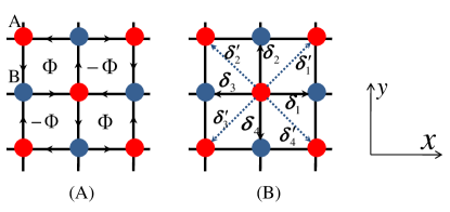
Figure 1: (Color online) $2$D Optical Raman lattice divided into two sublattices $A$ and $B$. (A) The nearest neighbour hopping caused by Raman potentials $V_{Rx}$ and $V_{Ry}$. (B) The four nearest neighbour vectors $\bm{\delta_{i}}(i=1,2,3,4)$ are connecting the two sublattices (solid arrows), and the four next nearest neighbour vectors $\bm{\delta^{\prime}_{i}}(i=1,2,3,4)$ are also shown (dashed arrows).

For the $s$-orbital bands, the Raman potential $V_{Rx}$ ($V_{Ry}$) leads to the hopping along $x$ ($y$) direction, which is accompanied by a phase $\phi_{y/x}$ ($-\phi_{y/x}$), when the hopping is toward (away from) $B$ sites. In experiment, we can readily set that $\phi_{x}=-\phi_{y}=\phi_{0}$, so the hopping along the paths described by arrows in Fig.1(A) acquires a phase $\phi_{0}$. This leads to a staggered flux configuration with the flux $|\Phi|=4\phi_{0}$ in each square plaquette. Moreover, owing to the odd parity of Raman potentials, the hopping from one site to its leftward (upward) neighboring site has an additional minus sign relative to the hopping to its rightward (downward) neighboring site.

With the above properties, we can obtain the $s$-band tight-binding Hamiltonian

$$H = -\sum_{\langle ij\rangle}(t_{ij}e^{i\phi_{ij}}\hat{c}_{b,i}^{\dagger}\hat{c}_{a,j}+{\rm H.c.})$$ (3)

$$-\sum_{\langle\langle ij\rangle\rangle}\sum_{\mu=a,b}t^{\prime}_{\mu,ij}\hat{c}_{\mu,i}^{\dagger}\hat{c}_{\mu,j}$$

$$+m_{z}\sum_{i}(\hat{c}^{\dagger}_{a,i}\hat{c}_{a,i}-\hat{c}^{\dagger}_{b,i}\hat{c}_{b,i}).$$

Here $\hat{c}_{\mu,i}$ is the fermionic annihilation operator on sublattice $A$ (for $\mu=a$) and $B$ (for $\mu=b$). The nearest neighbour vectors $\bm{\delta}_{1}(-\bm{\delta}_{3})=(a,0)$, $\bm{\delta}_{2}(-\bm{\delta}_{4})=(0,a)$ and the next nearest neighbour vectors $\bm{\delta}_{1}^{\prime}(-\bm{\delta}_{3}^{\prime})=(a,a)$, $\bm{\delta}_{2}^{\prime}(-\bm{\delta}_{4}^{\prime})=(-a,a)$ are shown in Fig.1(B), with $a$ the lattice constant. $\langle ij\rangle$ and $\langle\langle ij\rangle\rangle$ denote nearest neighbour and next nearest neighbour sites, respectively. The nearest neighbor and diagonal hopping coefficients, $t_{ij}$ and $t^{\prime}_{\mu,ij}$ have already been calculated in Ref.Liu et al. (2016). They satisfy $t_{i,i\pm 1_{x}}=\pm(-1)^{i_{x}}t_{0},t_{i,i\pm 1_{y}}=\mp(-1)^{i_{x}}t_{0},t^{\prime}_{\mu,ij}=t^{\prime}_{\mu}$, with $t_{0}=V_{R}\int d^{2}\mathbb{r}\psi_{b,s}^{(0,0)}(\mathbb{r})\cos(k_{1}x)\psi_{a,s}^{(1,0)}(\mathbb{r})$ and $t^{\prime}_{\mu}=\int d^{2}\mathbb{r}\psi_{\mu,s}^{(0,0)}(\mathbb{r})\bigr{[}\frac{\mathbb{p}^{2}}{2m}+V_{\rm sq}(\mathbb{r})\bigr{]}\psi_{\mu,s}^{(1,1)}(\mathbb{r})$ ($\mu=a,b$), where $\mathbb{p}$ is momentum of atom and $m$ is atom mass. The staggered sign $(-1)^{i_{x}}$ can be absorbed by transforming sublattice $B$ annihilation operator $\hat{c}_{b,j}$ into $e^{i\pi\frac{x_{j}}{a}}\hat{c}_{b,j}$. In terms of the new operator, the diagonal hopping coefficient $t^{\prime}_{b}$ acquires an additional minus sign $-t^{\prime}_{b}$. The hopping phase $\phi_{ij}=\nu_{ij}\phi_{0}$ with $\nu_{ij}=1$ ($-1$) for hopping along (opposite to) the marked direction in Fig.1(A), and the Zeeman term $m_{z}=\frac{\Delta-\delta\omega}{2}$. Furthermore, since $\psi_{a,s}$ and $\psi_{b,s}$ have the same spatial distribution, we may set $t^{\prime}_{a}\approx t^{\prime}_{b}$.

In order to diagonalize the Hamiltonian (3) we transform it into momentum space via

$$\hat{c}_{a,b}(\mathbb{r}_{i})=\frac{1}{\sqrt{N}}\sum_{\mathbb{k}}e^{i\mathbb{k}\cdot\mathbb{r}_{i}}\hat{c}_{a,b}(\mathbb{k}),$$ (4)

here $N$ is the number of unit cells, the sum over $\mathbb{k}$ is on the first Brillouin zone (FBZ). We get Hamiltonian in matrix form $H=\sum_{\mathbb{k}}\hat{\mathcal{C}}^{{\dagger}}(\mathbb{k})\mathcal{H}(\mathbb{k})\hat{\mathcal{C}}(\mathbb{k})$ with $\hat{\mathcal{C}}(\mathbb{k})=(\hat{c}_{a}(\mathbb{k}),\hat{c}_{b}(\mathbb{k}))^{T}$ and

$${\cal H}(\mathbb{k})=d_{x}(\mathbb{k})\sigma_{x}+d_{y}(\mathbb{k})\sigma_{y}+d_{z}(\mathbb{k})\sigma_{z},$$ (5)

with the coefficients

$$d_{x} = -2t_{0}\sin\phi_{0}(\sin k_{x}a+\sin k_{y}a),$$ (6)

$$d_{y} = -2t_{0}\cos\phi_{0}(\sin k_{x}a-\sin k_{y}a),$$ (7)

$$d_{z} = m_{z}-2(t^{\prime}_{a}+t^{\prime}_{b})\cos(k_{x}a)\cos(k_{y}a),$$ (8)

where $\sigma_{x,y,z}$ are three Pauli matrices for sublattices. It is clear that as long as $\phi_{0}\neq n\pi$ with $n\in\mathbb{Z}$, the time-reversal symmetry of system is broken, thus it can give rise to QAH effect.

Based on the band structure one can manifest QAH effect. The Hamiltonian has two energy bands given by $\mp\varepsilon=\mp\sqrt{d_{x}^{2}+d_{y}^{2}+d_{z}^{2}}$. Their corresponding eigenstates are (up to an arbitrary phase):

$$|u_{-}\rangle = \left(\begin{array}[]{c}\alpha_{-}\\[5.0pt] \beta_{-}\end{array}\right)=\left(\begin{array}[]{c}\sin\frac{\theta}{2}e^{-i\varphi}\\[5.0pt] -\cos\frac{\theta}{2}\end{array}\right),$$ (13)

$$|u_{+}\rangle = \left(\begin{array}[]{c}\alpha_{+}\\[5.0pt] \beta_{+}\end{array}\right)=\left(\begin{array}[]{c}\cos\frac{\theta}{2}e^{-i\varphi}\\[5.0pt] \sin\frac{\theta}{2}\end{array}\right),$$ (18)

where the mixing angles are defined by $\tan\theta=\frac{\sqrt{d_{x}^{2}+d_{y}^{2}}}{d_{z}}$, $\tan\varphi=\frac{d_{y}}{d_{x}}$. Now the Hamiltonian (3) can be diagonalized:

$$H = \sum_{\mathbb{k}}\big{(}\hat{c}^{\dagger}_{a}(\mathbb{k}),\hat{c}^{\dagger}_{b}(\mathbb{k})\big{)}\mathcal{H}(\mathbb{k})\left(\begin{array}[]{c}\hat{c}_{a}(\mathbb{k})\\[5.0pt] \hat{c}_{b}(\mathbb{k})\end{array}\right)$$ (21)

$$= \sum_{\mathbb{k}}\big{(}\hat{l}_{\mathbb{k}}^{\dagger},\hat{u}_{\mathbb{k}}^{\dagger}\big{)}\left(\begin{array}[]{cc}-\varepsilon&0\\[5.0pt] 0&\varepsilon\end{array}\right)\left(\begin{array}[]{c}\hat{l}_{\mathbb{k}}\\[5.0pt] \hat{u}_{\mathbb{k}}\end{array}\right),$$ (26)

here the new set of operators $\hat{l}_{\mathbb{k}}$ and $\hat{u}_{\mathbb{k}}$ associated with lower and upper bands are introduced.

To evaluate the gap, we find if $m_{z}$ is tuned from $m_{z}>2(t^{\prime}_{a}+t^{\prime}_{b})$ to $m_{z}=2(t^{\prime}_{a}+t^{\prime}_{b})$, the band gap is closed at Dirac point $\mathbb{k}=(0,0)$, and further tuning it from $m_{z}=2(t^{\prime}_{a}+t^{\prime}_{b})$ to $m_{z}<2(t^{\prime}_{a}+t^{\prime}_{b})$, the gap is reopened. Similarly, adjusting $m_{z}$ from $m_{z}<-2(t^{\prime}_{a}+t^{\prime}_{b})$ to $m_{z}>-2(t^{\prime}_{a}+t^{\prime}_{b})$, the gap is closed and then reopened at Dirac point $\mathbb{k}=(0,\frac{\pi}{a})$.

If the Fermi energy (chemical potential) lies in the gap, only the lower band is occupied, we may use the eigenstate $|u_{-}\rangle$ to calculate the anomalous Hall conductivity (AHC), which reads:

$$\sigma^{H}_{xy}=\frac{1}{h}\int_{{\rm FBZ}}dk_{x}dk_{y}\frac{\mathbb{n}\cdot(\partial_{k_{x}}\mathbb{n}\times\partial_{k_{y}}\mathbb{n})}{4\pi}=\frac{C_{1}}{h},$$ (27)

where $\mathbb{n}=(d_{x},d_{y},d_{z})/(d_{x}^{2}+d_{y}^{2}+d_{z}^{2})^{1/2}$. $C_{1}$ is the first Chern number, a quantized topological invariant Kohmoto (1985); Xiao et al. (2010) defined on the FBZ. By derivation one can show

$$C_{1} = +1,\text{for $0<\phi_{0}<\frac{\pi}{2},|m_{z}|<2(t^{\prime}_{a}+t^{\prime}_{b})$,}$$

$$C_{1} = -1,\text{for $\frac{\pi}{2}<\phi_{0}<\pi,|m_{z}|<2(t^{\prime}_{a}+t^{\prime}_{b})$,}$$

$$C_{1} = 0,~{}~{}\text{for $\phi_{0}=\frac{n\pi}{2}(n\in\mathbb{Z})$ or $|m_{z}|>2(t^{\prime}_{a}+t^{\prime}_{b})$.}$$

It indicates that topological phase (QAH insulator) exists only when $|m_{z}|<2(t^{\prime}_{a}+t^{\prime}_{b})$ and $\phi_{0}\neq\frac{n\pi}{2}(n\in\mathbb{Z})$. which has gapped bulk states Liu et al. (2016) but supports gapless edge states on the boundaries of the system Liu et al. (2010).

Next we will take into account a spin-$\frac{1}{2}$ two-copy version of QAH model. The two copies can be obtained from two subspaces $\Gamma_{1}$ and $\Gamma_{2}$ of a system. $\Gamma_{1}$ subspace is described by a Hamiltonian corresponding to spin-up state:

$$H_{\Gamma_{1}}=\sum_{\mathbb{k}}\big{(}\hat{c}^{\dagger}_{a\uparrow}(\mathbb{k}),\hat{c}^{\dagger}_{b\uparrow}(\mathbb{k})\big{)}\mathcal{H}(\mathbb{k})\left(\begin{array}[]{c}\hat{c}_{a\uparrow}(\mathbb{k})\\[5.0pt] \hat{c}_{b\uparrow}(\mathbb{k})\end{array}\right),$$ (29)

and $\Gamma_{2}$ subspace is described by a Hamiltonian corresponding to spin-down state:

$$H_{\Gamma_{2}}=\sum_{\mathbb{k}}\big{(}\hat{c}^{\dagger}_{a\downarrow}(\mathbb{k}),\hat{c}^{\dagger}_{b\downarrow}(\mathbb{k})\big{)}\mathcal{H}(\mathbb{k})\left(\begin{array}[]{c}\hat{c}_{a\downarrow}(\mathbb{k})\\[5.0pt] \hat{c}_{b\downarrow}(\mathbb{k})\end{array}\right),$$ (30)

here in Eqs.(29) and (30), $\mathcal{H}(\mathbb{k})$ is given by Eq.(5). When Fermi energy is inside the gap and both $\Gamma_{1}$ and $\Gamma_{2}$ subsystems are half filled, each subspace forms a QAH insulator with the same Chern number. Since $\Gamma_{1}$ and $\Gamma_{2}$ subspaces decouple, we have the total Hamiltonian: $H=\sum_{\mathbb{k}}\hat{\mathcal{C}}^{{\dagger}}(\mathbb{k})\mathcal{H}(\mathbb{k})\hat{\mathcal{C}}(\mathbb{k})$ with $\hat{\mathcal{C}}(\mathbb{k})=(\hat{c}_{a\uparrow}(\mathbb{k}),\hat{c}_{b\uparrow}(\mathbb{k}),\hat{c}_{a\downarrow}(\mathbb{k}),\hat{c}_{b\downarrow}(\mathbb{k}))^{T}$ and

$$\mathcal{H}(\mathbb{k}) = \sum_{\alpha=x,y,z}d_{\alpha}(\mathbb{k})I\otimes\sigma_{\alpha}.$$ (31)

The main task of this paper is to investigate the effect of a repulsive Fermi Hubbard interaction on the above spin-$\frac{1}{2}$ two-copy version of QAH model. The Hubbard term can be written as:

$$H_{I}=U\sum_{i}n_{i\uparrow}n_{i\downarrow}\ ,$$ (32)

where $U$ is the strength of Hubbard interaction. In the case of half filling we may rewrite the Hubbard interaction as

$$H_{I}=\frac{U}{2}\sum_{i}\left(\sum_{\sigma}n_{i\sigma}-1\right)^{2}\ .$$ (33)

This formulation often appears in the slave-rotor theory. In what follows, we set lattice constant $a=1$, next nearest neighbour hopping coefficients $t^{\prime}_{a}=t^{\prime}_{b}=t_{1}$ and the Zeeman term $m_{z}=0$ for resonant Raman process.

III slave-rotor mean-field formalism

Now we give the general idea of slave-rotor approach. According to Ref. Florens and Georges (2002, 2004); Zhao and Paramekanti (2007), the original fermion operator $\hat{c}_{i\sigma}$ will be rewritten by a product of a spin-$\frac{1}{2}$ spinon (auxiliary fermion) operator $\hat{f}_{i\sigma}$ and a charged rotor $e^{i\theta_{i}}$,

$$\hat{c}_{i\sigma}=e^{i\theta_{i}}\hat{f}_{i\sigma}.$$ (34)

Based on this representation, the phase variable $\theta_{i}$ is conjugate to the total charge. In terms of the new variable, the quartic Hubbard interaction term (33) between the fermions is expressed by a simple kinetic term $\widehat{L}^{2}$, where the angular momentum operator $\widehat{L}\propto i\partial_{\theta}$ is associated with a quantum O(2) rotor field $\theta$. State vectors in the new Hilbert space take the form $|\Psi\rangle=|\Psi_{f}\rangle|\Psi_{\theta}\rangle$. The new rotor-spinon Hilbert space is enlarged compared to the original one since there exist unphysical states. To eliminate these unphysical states we have to impose a constraint about operators,

$$\sum_{\sigma}\hat{f}_{i\sigma}^{\dagger}\hat{f}_{i\sigma}^{\phantom{\dagger}}+\widehat{L}_{i}=1\ .$$ (35)

The hopping terms of Hamiltonian are rewritten as

$$H = -\sum_{\langle ij\rangle\sigma}t_{ij}e^{i\phi_{ij}}\hat{f}_{i\sigma}^{\dagger}\hat{f}_{j\sigma}e^{-i\theta_{ij}}$$ (36)

$$-\sum_{\langle\langle ij\rangle\rangle}\sum_{\sigma}t_{1}\hat{f}_{i\sigma}^{\dagger}\hat{f}_{j\sigma}e^{-i\theta_{ij}},$$

where $\theta_{ij}\equiv\theta_{i}-\theta_{j}$. Moreover, we replace the phase field $e^{i\theta_{i}}$ representing the O($2$) degree of freedom by a complex bosonic field $X_{i}(\tau)$ which is constrained by

$$|X_{i}(\tau)|^{2}=1,$$ (37)

here the imaginary time $\tau=it$.

The above mean-field formalism can be used to treat correlated fermionic systems at moderate interactions, where the bosonic field $X_{i}(\tau)$ is related to Mott transition.

IV Transition from QAH state to CSL

In this section we use the slave-rotor mean-field formalism to determine the phase boundary between QAH state and CSL. In QAH state, the rotor is condensed and the original fermion operator $\hat{c}_{i\sigma}$ is proportional to the spinon operator $\hat{f}_{i\sigma}$. In other words, the degrees of freedom of rotor and spinon are not separated. The whole system is a QAH insulator. While in the CSL state , the charge degrees of freedom form a Mott insulator state, but the spinon is described by a Hamiltonian which is very similar to the Hamiltonian (31) of the spin-$\frac{1}{2}$ two-copy version of QAH model. In this respect the rotor undergoes a phase transition from superfluid to Mott insulator. Furthermore, no symmetry breaking orders (such as magnetic orders) appear in the CSL state.

The Hubbard interaction term (33) is rewritten in terms of the new variables $e^{i\theta_{i}}$ and $\hat{f}_{i\sigma}$ as

$$H_{I}=\frac{U}{2}\sum_{i}\left(\sum_{\sigma}n_{i\sigma}-1\right)^{2}=\frac{U}{2}\sum_{i}\widehat{L}_{i}^{2},$$ (38)

where we use the constraint (35) and $n_{i\sigma}=\hat{f}^{\dagger}_{i\sigma}\hat{f}_{i\sigma}$.

The slave-rotor Hamiltonian reads

$$H = -\sum_{\langle ij\rangle\sigma}t_{ij}e^{i\phi_{ij}}\hat{f}_{i\sigma}^{\dagger}\hat{f}_{j\sigma}e^{-i\theta_{ij}}$$ (39)

$$-\sum_{\langle\langle ij\rangle\rangle}\sum_{\sigma}t_{1}\hat{f}_{i\sigma}^{\dagger}\hat{f}_{j\sigma}e^{-i\theta_{ij}}$$

$$-\mu\sum_{i,\sigma}\hat{f}^{\dagger}_{i\sigma}\hat{f}_{i\sigma}+\frac{U}{2}\sum_{i}\widehat{L}_{i}^{2}.$$

where $\mu$ is chemical potential. Then the mean-field decomposed action is

$$S_{0} = \int_{0}^{\beta}d\tau\Big{[}\sum_{i\sigma}\hat{f}_{i\sigma}^{\dagger}\left(\partial_{\tau}-\mu+h_{i}\right)\hat{f}_{i\sigma}+\sum_{i}\rho|X_{i}|^{2}$$

$$+\frac{1}{2U}\sum_{i}[(i\partial_{\tau}+ih_{i})X_{i}^{\ast}][(-i\partial_{\tau}+ih_{i})X_{i}]$$

$$+\sum_{i}\left(-h_{i}+\frac{h_{i}^{2}}{2U}\right)+H_{X}+H_{X}^{\prime}+H_{f}+H_{f}^{\prime}\Big{]},$$

here $\beta=\frac{1}{k_{B}T}=\frac{\tau}{\hbar}$. We have to fulfill the constraints (35) and (37) with the Lagrange multipliers $h_{i}$ and $\rho$, respectively.

Since it contains $A$, $B$ sublattices, the effective Hamiltonians for rotor and spinon parts are

$$H_{X} = -Q_{X}\sum_{\langle ij\rangle}X_{i}^{b\ast}X_{j}^{a}+{\rm c.c.},$$ (41)

$$H_{f} = -Q_{f}\sum_{\langle ij\rangle\sigma}t_{ij}e^{i\phi_{ij}}\hat{f}_{i\sigma}^{{\dagger}}\hat{f}_{j\sigma}+{\rm H.c.},$$ (42)

$$H_{X}^{\prime} = -Q_{X}^{\prime}\sum_{\langle\langle ij\rangle\rangle}X_{i}^{\ast}X_{j},$$ (43)

$$H_{f}^{\prime} = -Q_{f}^{\prime}\sum_{\langle\langle ij\rangle\rangle}\sum_{\sigma}t_{1}\hat{f}_{i\sigma}^{\dagger}\hat{f}_{j\sigma}.$$ (44)

The mean-field parameters associated with the decomposition are given by

$$Q_{X} = \langle\sum_{\sigma}t_{ij}e^{i\phi_{ij}}\hat{f}_{i\sigma}^{b{\dagger}}\hat{f}_{j\sigma}^{a}\rangle,$$ (45)

$$Q_{f} = \langle X_{i}^{\ast}X_{j}\rangle,$$ (46)

for the nearest neighbour hopping and

$$Q_{X}^{\prime} = \langle\sum_{\sigma}t_{1}\hat{f}_{i\sigma}^{\dagger}\hat{f}_{j\sigma}\rangle,$$ (47)

$$Q_{f}^{\prime} = \langle X_{i}^{\ast}X_{j}\rangle$$ (48)

for the next nearest neighbour hopping. Note that we consider only the half filled case which allowed us to set $\mu=h_{i}=0$.

For the spinon Hamiltonian,

$$H_{f}+H_{f}^{\prime}$$ (49)

$$= \sum_{\mathbb{k}}\Phi^{\dagger}_{\mathbb{k}}I\otimes(Q_{f}d_{x}\sigma_{x}+Q_{f}d_{y}\sigma_{y}+Q_{f}^{\prime}d_{z}\sigma_{z})\Phi_{\mathbb{k}}$$

$$= \sum_{\mathbb{k}\sigma}(-\Sigma_{\mathbb{k}}\,{f_{\mathbb{k}\sigma}^{l\dagger}}{f_{\mathbb{k}\sigma}^{l}}+\Sigma_{\mathbb{k}}\,{f_{\mathbb{k}\sigma}^{u\dagger}}{f_{\mathbb{k}\sigma}^{u}}),$$

here $\Phi^{\dagger}_{\mathbb{k}}=(f_{\mathbb{k}\uparrow}^{a\dagger},f_{\mathbb{k}\uparrow}^{b\dagger},f_{\mathbb{k}\downarrow}^{a\dagger},f_{\mathbb{k}\downarrow}^{b\dagger})$. Thus, we obtain the renormalized spinon band structure

$$\Sigma_{\mathbb{k}}=\sqrt{Q_{f}^{2}(d_{x}^{2}+d_{y}^{2})+(Q_{f}^{\prime}d_{z})^{2}},$$ (50)

which is very similar to that of spin-$\frac{1}{2}$ two-copy version of QAH model.

For the rotor Hamiltonian,

$$H_{X} = Q_{X}\sum_{\mathbb{k}}[-|g_{1}|{X_{\mathbb{k}}^{l\ast}}{X_{\mathbb{k}}^{l}}+|g_{1}|{X_{\mathbb{k}}^{u\ast}}{X_{\mathbb{k}}^{u}}\ ],$$ (51)

$$H_{X}^{\prime} = -Q_{X}^{\prime}\sum_{\mathbb{k}}g_{2}(\mathbb{k})({X_{\mathbb{k}}^{l\ast}}{X_{\mathbb{k}}^{l}}+{X_{\mathbb{k}}^{u\ast}}{X_{\mathbb{k}}^{u}})\ ,$$ (52)

the Green function for the $X$ fields is written as

$$G_{X}=\frac{1}{\frac{\nu_{n}^{2}}{2U}+\rho+\xi_{\mathbb{k}}},$$ (53)

here we ignore the upper band of rotor and consider only the lower band

$$\xi_{\mathbb{k}}=-Q_{X}|g_{1}(\mathbb{k})|-Q_{X}^{\prime}g_{2}(\mathbb{k}),$$ (54)

with $g_{1}(\mathbb{k})=\sum_{i=1}^{4}e^{-i\mathbb{k}\cdot\bm{\delta}_{i}}$, $g_{2}(\mathbb{k})=\sum_{i=1}^{4}e^{-i\mathbb{k}\cdot\bm{\delta}_{i}^{\prime}}$, and bosonic Matsubara frequency $\nu_{n}$.

To treat the constraint (37) on average, we find a self-consistency equation:

$$1 = \frac{1}{N}\sum_{\mathbb{k}}\frac{1}{\beta}\sum_{n}G_{X}(\mathbb{k},\nu_{n})$$ (55)

$$= \frac{\sqrt{2}U}{N}\sum_{\mathbb{k}}\frac{1}{\sqrt{\Delta_{X}^{2}+4U[\xi_{\mathbb{k}}-\min(\xi_{\mathbb{k}})]}}$$

by introducing the insulating gap of rotor

$$\Delta_{X}=2\sqrt{U[\rho+\min{(\xi_{\mathbb{k}})}]}\ .$$ (56)

If the phase transition from the Mott insulator to the superfluid of the rotor takes place, the rotor gap $\Delta_{X}$ must close. It indicates that

$$U_{c_{1}}(t_{1})=\frac{1}{2}\left[\frac{1}{2N}\sum_{\mathbb{k}^{\prime}}\frac{1}{\sqrt{\xi_{\mathbb{k}}-\min(\xi_{\mathbb{k}})}}\right]^{-2}\ ,$$ (57)

which defines the critical interaction strength of Mott insulator, i.e when $U\leq U_{c_{1}},\Delta_{X}=0$; $U>U_{c_{1}},\Delta_{X}>0$.

After some detailed calculation (see appendix A), we may solve the mean field equations corresponding to (45), (46), (47), (48) and (57) self consistently along the phase boundary $U_{c_{1}}$. The mean-field parameters ($Q_{X}$, $Q_{X}^{\prime}$, $Q_{f}^{c}$, $Q_{f}^{\prime c}$) as functions of next nearest hopping coefficient $t_{1}$ are plotted in Fig.2. Here the hopping phase $\phi_{0}=\frac{\pi}{4}$ such that the flux $|\Phi|=\pi$ in each square plaquette in Fig. 1(A).

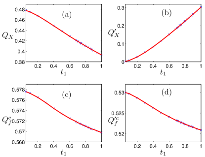
Figure 2: (Color online)Numerical solutions of the mean-field parameters (45), (46), (47) and (48) ($t_{0}=1$) along the phase boundary $U_{c_{1}}$: (a) $Q_{X}(t_{1})$, (b)$Q^{\prime}_{X}(t_{1})$, (c)$Q_{f}^{c}(t_{1})$, (d)$Q_{f}^{\prime c}(t_{1})$.

It is shown that along the phase transition from QAH state to CSL, with $t_{1}$ increasing from $0.05$ to $1$, $Q^{\prime}_{X}$ increases from nearly zero to about $0.3$, but $Q_{X}$, $Q_{f}^{c}$ and $Q_{f}^{\prime c}$ decrease. Moreover, both $Q_{f}^{c}$ and $Q_{f}^{\prime c}$ decrease very slowly.

V Transition from CSL state to magnetic phase

Since the system may contain symmetry breaking orders at some parameter region, we may introduce magnetic order parameters $m_{1}$ and $m_{2}$ to describe Neel order and stripe order, respectively, which are two typical symmetry breaking orders. In the Neel order, the staggered spin order exists in the $x$ and $y$ directions [Fig.3(A)]. While in the stripe order, the staggered spin order exists only in the $x$ or $y$ direction [Fig.3(B)].

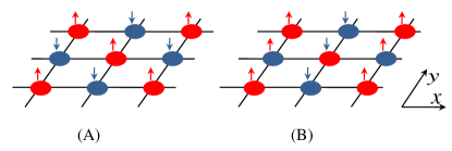
Figure 3: (Color online) (A) The Neel order, (B) The stripe order.

If we consider Neel state and stripe state at the same time, the square lattice can be divided into four sublattices ($A,B,C,D$), the area of unit cell is enlarged to be twice as large as the area of original unit cell without magnetic order. Hence, the area of the corresponding FBZ is reduced to be half of area of the original FBZ. The new FBZ is called reduced Brillouin zone (RBZ). The sum over $\mathbb{k}$ on the RBZ is denoted as $\sum_{\mathbb{k}\in\,{\rm RBZ}}$, and the number of unit cells is $N_{0}$. The magnetic order parameters are generally written as

$$\langle n_{i\uparrow}-n_{i\downarrow}\rangle=\frac{1}{2}[(-1)^{i_{x}+i_{y}}m_{1}+(-1)^{i_{x}}m_{2}],$$ (58)

with $i_{x}=\frac{x_{i}}{a}$, $i_{y}=\frac{y_{i}}{a}$.

As mentioned in section III, in the slave-rotor representation, the original fermion operator can be rewritten by using spinon operator $\hat{f}_{i\sigma}$ and rotor field $e^{i\theta_{i}}$: $\hat{c}_{i\sigma}=e^{i\theta_{i}}\hat{f}_{i\sigma}$. The mean-field decomposed action takes the following form

$$S_{0} = \int_{0}^{\beta}d\tau\Big{[}\sum_{i\sigma}\hat{f}_{i\sigma}^{\dagger}\left(\partial_{\tau}-\mu+h_{i}\right)\hat{f}_{i\sigma}+\sum_{i}\rho|X_{i}|^{2}$$ (59)

$$+\frac{1}{2U}\sum_{i}[(i\partial_{\tau}+ih_{i})X_{i}^{\ast}][(-i\partial_{\tau}+ih_{i})X_{i}]$$

$$+\sum_{i}\left(-h_{i}+\frac{h_{i}^{2}}{2U}\right)+H_{X}+H_{X}^{\prime}+H_{f}+H_{f}^{\prime}$$

$$+H_{f}^{\prime\prime}\Big{]}$$

with

$$H_{X} = -\langle\sum_{\sigma}t_{ij}e^{i\phi_{ij}}\hat{f}_{i\sigma}^{{\dagger}}\hat{f}_{j\sigma}\rangle\sum_{\langle ij\rangle}X_{i}^{\ast}X_{j}+{\rm c.c.}$$ (60)

$$= -Q_{X_{1}}\sum_{i}X_{i}^{\ast}X_{i\pm 1_{x}}$$

$$-Q_{X_{2}}\sum_{i}X_{i}^{\ast}X_{i\pm 1_{y}}+{\rm c.c.},$$

$$H_{f} = -Q_{f}\sum_{\langle ij\rangle\sigma}t_{ij}e^{i\phi_{ij}}\hat{f}_{i\sigma}^{{\dagger}}\hat{f}_{j\sigma}+{\rm H.c.},$$ (61)

$$H_{X}^{\prime} = -Q_{X}^{\prime}\sum_{\langle\langle ij\rangle\rangle}X_{i}^{\ast}X_{j},$$ (62)

$$H_{f}^{\prime} = -Q_{f}^{\prime}\sum_{\langle\langle ij\rangle\rangle}\sum_{\sigma}t_{1}\hat{f}_{i\sigma}^{\dagger}\hat{f}_{j\sigma},$$ (63)

$$H_{f}^{\prime\prime} = -\frac{U}{4}\sum_{i}[(-1)^{i_{x}+i_{y}}m_{1}+(-1)^{i_{x}}m_{2}]$$ (64)

$$\cdot(\hat{f}_{i\uparrow}^{\dagger}\hat{f}_{i\uparrow}^{\phantom{\dagger}}-\hat{f}_{i\downarrow}^{\dagger}\hat{f}_{i\downarrow}^{\phantom{\dagger}})+\frac{UN_{0}}{4}(m_{1}^{2}+m_{2}^{2})+c,$$

here $\frac{U}{4}\sum_{i}n_{i}^{2}=c$ is a constant, $n_{i}=n_{i\uparrow}+n_{i\downarrow}$. We still fulfill the constraints (35) and (37) with the Lagrange multipliers $h_{i}$ and $\rho$, respectively . The magnetic orders break spin rotation symmetry and only affect spinon degrees of freedom, so the square lattice can be divided into four sublattices ($A,B,C,D$) for spinon, the sum over $\mathbb{k}$ is denoted as $\sum_{\mathbb{k}\in\,{\rm RBZ}}$. But for the rotor, the square lattice still has two sublattices ($A,B$), the sum over $\mathbb{k}$ is still on the original FBZ and denoted as $\sum_{\mathbb{k}}$.

The mean-field parameters associated with the decomposition are given by

$$Q_{X_{1}} = \langle\sum_{\sigma}t_{ij}e^{i\phi_{ij}}\hat{f}_{i\sigma}^{b{\dagger}}\hat{f}_{j\sigma}^{a}\rangle=\langle\sum_{\sigma}t_{ij}e^{i\phi_{ij}}\hat{f}_{i\sigma}^{d{\dagger}}\hat{f}_{j\sigma}^{c}\rangle,$$

$$Q_{X_{2}} = \langle\sum_{\sigma}t_{ij}e^{i\phi_{ij}}\hat{f}_{i\sigma}^{d{\dagger}}\hat{f}_{j\sigma}^{a}\rangle=\langle\sum_{\sigma}t_{ij}e^{i\phi_{ij}}\hat{f}_{i\sigma}^{b{\dagger}}\hat{f}_{j\sigma}^{c}\rangle,$$

$$Q_{f} = \langle X_{i}^{\ast}X_{j}\rangle,$$ (67)

for the nearest neighbour hopping and

$$Q_{X}^{\prime} = \langle\sum_{\sigma}t_{1}\hat{f}_{i\sigma}^{\dagger}\hat{f}_{j\sigma}\rangle,$$ (68)

$$Q_{f}^{\prime} = \langle X_{i}^{\ast}X_{j}\rangle$$ (69)

for the next nearest neighbour hopping. We still have $\mu=h_{i}=0$ for half filled case.

The spinon Hamiltonian in momentum space is written as

$$H_{f}+H_{f}^{\prime}+H_{f}^{\prime\prime}$$ (70)

$$= \sum_{\mathbb{k}\in\,{\rm RBZ},\sigma}\Phi_{\mathbb{k}\sigma}^{\dagger}\mathcal{H}_{\sigma}\Phi_{\mathbb{k}\sigma}+\frac{UN_{0}}{4}(m_{1}^{2}+m_{2}^{2})+c$$

$$= \sum_{\mathbb{k}\in\,{\rm RBZ},\sigma}(-\Sigma_{1}\hat{f}_{\mathbb{k}\sigma}^{l_{1}\dagger}\hat{f}_{\mathbb{k}\sigma}^{l_{1}}-\Sigma_{2}\hat{f}_{\mathbb{k}\sigma}^{l_{2}\dagger}\hat{f}_{\mathbb{k}\sigma}^{l_{2}}$$

$$+\Sigma_{2}\hat{f}_{\mathbb{k}\sigma}^{u_{1}\dagger}\hat{f}_{\mathbb{k}\sigma}^{u_{1}}+\Sigma_{1}\hat{f}_{\mathbb{k}\sigma}^{u_{2}\dagger}\hat{f}_{\mathbb{k}\sigma}^{u_{2}})$$

$$+\frac{UN_{0}}{4}(m_{1}^{2}+m_{2}^{2})+c,$$

here $\Phi_{\mathbb{k}\sigma}=(\hat{f}_{\mathbb{k}\sigma}^{a},\hat{f}_{\mathbb{k}\sigma}^{b},\hat{f}_{\mathbb{k}\sigma}^{c},\hat{f}_{\mathbb{k}\sigma}^{d})$, $\mathcal{H}_{\uparrow}$ and $\mathcal{H}_{\downarrow}$ are two $4\times 4$ matrices presented in appendix A. We get the renormalized mean-field free energy at $T=0$ for spinon sector

$$\mathcal{F}=\sum_{\mathbb{k}\in\,{\rm RBZ}}(-2\Sigma_{1}-2\Sigma_{2})+\frac{UN_{0}}{4}(m_{1}^{2}+m_{2}^{2})+c.$$ (71)

The self-consistency equations about magnetic orders $m_{1}$ and $m_{2}$ are equivalent to energy extreme conditions $\frac{\partial\mathcal{F}}{\partial m_{1}}=\frac{\partial\mathcal{F}}{\partial m_{2}}=0$. By solving them we may determine critical interaction strength $U_{c_{2}}$ of magnetic order, i.e. when $U>U_{c_{2}}$, $m_{1}\neq 0,m_{2}=0$ (Neel state) or $m_{1}=0,m_{2}\neq 0$ (stripe state); when $U\leq U_{c_{2}}$, $m_{1}=m_{2}=0$ (CSL).

For the rotor Hamiltonian

$$H_{X} = \sum_{\mathbb{k}}[-|g(\mathbb{k})|{X_{\mathbb{k}}^{l\ast}}{X_{\mathbb{k}}^{l}}+|g(\mathbb{k})|{X_{\mathbb{k}}^{u\ast}}{X_{\mathbb{k}}^{u}}\ ],$$ (72)

$$H_{X}^{\prime} = -Q_{X}^{\prime}\sum_{\mathbb{k}}g_{2}(\mathbb{k})({X_{\mathbb{k}}^{l\ast}}{X_{\mathbb{k}}^{l}}+{X_{\mathbb{k}}^{u\ast}}{X_{\mathbb{k}}^{u}})\ ,$$ (73)

where $g(\mathbb{k})=2[Q_{X_{1}}\cos(k_{x}a)+Q_{X_{2}}\cos(k_{y}a)]$, $g_{2}(\mathbb{k})=\sum_{i=1}^{4}e^{-i\mathbb{k}\cdot\bm{\delta}_{i}^{\prime}}$, the Green function for the $X$ fields is written as

$$G_{X}=\frac{1}{\frac{\nu_{n}^{2}}{2U}+\rho+\xi_{\mathbb{k}}}$$ (74)

where we consider the lower band of rotor

$$\xi_{\mathbb{k}}=-2|Q_{X_{1}}\cos(k_{x}a)+Q_{X_{2}}\cos(k_{y}a)|-Q_{X}^{\prime}g_{2}(\mathbb{k}),$$ (75)

with bosonic Matsubara frequency $\nu_{n}$.

From the constraint (37) we have the following self-consistency equation along the phase boundary $U_{c_{2}}$

$$1=\frac{1}{N}\sum_{\mathbb{k}}\frac{1}{\beta}\sum_{n}G_{X}(\mathbb{k},\nu_{n})=\frac{\sqrt{2U_{c_{2}}}}{2N}\sum_{\mathbb{k}}\frac{1}{\sqrt{\rho+\xi_{\mathbb{k}}}}.$$ (76)

We can solve the equation to get Lagrange multiplier $\rho_{c}$. It can be found $\rho_{c}>-\min{(\xi_{\mathbb{k}})}$, so the insulating gap of rotor $\Delta_{X}=2\sqrt{U[\rho+\min{(\xi_{\mathbb{k}})}]}$ is nonzero.

We still set hopping phase $\phi_{0}=\frac{\pi}{4}$. Equations $\frac{\partial\mathcal{F}}{\partial m_{1}}=\frac{\partial\mathcal{F}}{\partial m_{2}}=0$, (V), (V),(67),(68), (69), and (76) can be solved self consistently (see appendix A). After careful numerical calculation we find (V) is equal to (V) along the phase transition from CSL to magnetic phase, so we have $Q_{X_{1}}=Q_{X_{2}}\equiv Q_{X}$. We plot the mean-field parameters $Q_{X}$, $Q^{\prime}_{X}$, $Q_{f}^{c}$ and $Q_{f}^{\prime c}$ as functions of $t_{1}$ in Fig.4.

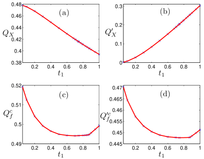
Figure 4: (Color online) Numerical solutions of the mean-field parameters (V)((V)), (67),(68) and (69) ($t_{0}=1$) along the phase boundary $U_{c_{2}}$: (a) $Q_{X}(t_{1})$, (b)$Q^{\prime}_{X}(t_{1})$, (c)$Q_{f}^{c}(t_{1})$, (d)$Q_{f}^{\prime c}(t_{1})$.

Comparing Fig.4 with Fig.2, with $t_{1}$ increasing from $0.05$ to $1$, along the phase transition from CSL to magnetic phase, the behaviors of $Q_{X}$ and $Q^{\prime}_{X}$ are very similar to those of $Q_{X}$ and $Q^{\prime}_{X}$ along the phase transition from QAH state to CSL. As for the behaviors of $Q_{f}^{c}$ and $Q_{f}^{\prime c}$ , different from Figs.2 (c) and (d), at the phase boundary of magnetic order, when $t_{1}<0.87$ both $Q_{f}^{c}$ and $Q_{f}^{\prime c}$ decrease at first, then vary very smoothly. But when $t_{1}>0.87$, they increase slowly. It indicates that magnetic order affects the spinon Hamiltonian, but not the rotor one.

VI mean-field phase diagram of CSL in Fermi Hubbard model

The self-consistency solutions of equations (57), $\frac{\partial\mathcal{F}}{\partial m_{1}}=\frac{\partial\mathcal{F}}{\partial m_{2}}=0$ give critical interaction strength of CSL as functions of $t_{1}$ in Fig.5.

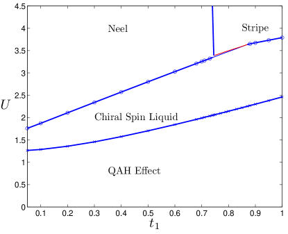
Figure 5: (Color online) The slave-rotor mean-field phase diagram versus $t_{1}$ and Hubbard interaction $U$ of the optical Raman lattice. It has been set $t_{0}=1$.

It can be seen that when the strength of Hubbard interaction reaches a critical value $U_{c_{1}}$, the system will experience a phase transition from QAH state to CSL state. During this transition, the spin and charge are separated from each other. The charge degrees of freedom are frozen in the Mott insulator phase, while spinon degrees of freedom are described by the Hamiltonian (49), which is exactly the spin-$\frac{1}{2}$ two-copy version of QAH model. This transition line corresponds to the lower boundary of CSL in Fig.5.

Since no magnetic order exists in the CSL phase, the CSL-magnetic phase transition will take place when interaction strength further increases and reaches another critical value $U_{c_{2}}$. This corresponds to the upper boundary of CSL in Fig.5. Along this transition line, when $0.05\leq t_{1}<0.87$, the CSL-Neel transition occurs first; when $0.87<t_{1}\leq 1$, the CSL-stripe transition occurs first. The three phases meet at a point ($t_{1}=0.87,U=3.635$). When $0.745\leq t_{1}<0.87$, a Neel-stripe transition (the red line in Fig.5) will take place after CSL-Neel transition if interaction strength increases to a slightly larger critical value $U_{c_{3}}>U_{c_{2}}$, i.e. when $U_{c_{2}}<U\leq U_{c_{3}}$, $m_{1}\neq 0,m_{2}=0$ (Neel state); when $U>U_{c_{3}}$, $m_{1}=0,m_{2}\neq 0$ (stripe state).

VII chiral spin liquid phase in effective spin model

It is well known that when $U$ is large in the Hubbard interaction term (32), each lattice site can not be doubly occupied, so the system is in a Mott insulator state. We can derive an effective spin model by considering the Hilbert space with single occupied sites and treating the hopping terms as perturbations. In this section we will investigate the effective spin model and give more reasonable CSL phase diagram at mean-field level. Note that we can only give the phase boundary between CSL phase and magnetic phase by using the effective spin model. As for the transition from QAH state to CSL, we still use the results obtained from the slave rotor formalism, i.e. the lower boundary $U_{c_{1}}$ of CSL in Fig.5).

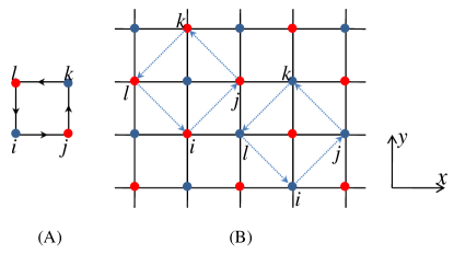
Figure 6: (Color online)Schematic illustration of four spin interactions, each spin is interacted only once, (A)only nearest neighbour hopping, $\phi_{ijkl}=\pi$; (B)only next nearest neighbour hopping, $\phi_{ijkl}=0$.

As emphasized in section I, the time-reversal symmetry of the system is broken in the CSL phase, so the effective spin model should at least include the terms up to third order perturbation expansions of $\frac{t_{0}}{U}$ and $\frac{t_{1}}{U}$, which correspond to interactions of three spins located at lattice sites of a closed minimum triangular loop. As for the fourth order expansions, they are exactly the four spin interaction terms. Relevant four spin interaction terms have also important effect on CSL phase, thus these terms should also be considered. The derivation of effective spin model up to fourth order correction is presented in appendix B. Considering all spin configurations we can get the following effective Hamiltonian for the spin degrees of freedom with $t_{0},t_{1}$ being small compared with $U$ MacDonald et al. (1988)

$$H_{\rm eff} = \sum_{\langle ij\rangle}\frac{4t_{0}^{2}}{U}\mathbf{S}_{i}\cdot\mathbf{S}_{j}+\sum_{\langle\langle ij\rangle\rangle}\frac{4t_{1}^{2}}{U}\mathbf{S}_{i}\cdot\mathbf{S}_{j}+\sum_{ijk\in\bigtriangleup}\frac{24t_{0}^{2}t_{1}}{U^{2}}\sin(\phi_{ijk})\mathbf{S}_{i}\cdot(\mathbf{S}_{j}\times\mathbf{S}_{k})$$ (77)

$$+\frac{t_{0}^{4}}{U^{3}}\sum_{ijkl\in\Box}\cos(\phi_{ijkl})\{80[(\mathbf{S}_{i}\cdot\mathbf{S}_{j})(\mathbf{S}_{k}\cdot\mathbf{S}_{l})+(\mathbf{S}_{i}\cdot\mathbf{S}_{l})(\mathbf{S}_{j}\cdot\mathbf{S}_{k})-(\mathbf{S}_{i}\cdot\mathbf{S}_{k})(\mathbf{S}_{j}\cdot\mathbf{S}_{l})]$$

$$-4(\mathbf{S}_{i}\cdot\mathbf{S}_{j}+\mathbf{S}_{k}\cdot\mathbf{S}_{l}+\mathbf{S}_{j}\cdot\mathbf{S}_{k}+\mathbf{S}_{i}\cdot\mathbf{S}_{l}+\mathbf{S}_{i}\cdot\mathbf{S}_{k}+\mathbf{S}_{j}\cdot\mathbf{S}_{l})\}$$

$$+\frac{t_{1}^{4}}{U^{3}}\sum_{ijkl\in\diamond}\{80[(\mathbf{S}_{i}\cdot\mathbf{S}_{j})(\mathbf{S}_{k}\cdot\mathbf{S}_{l})+(\mathbf{S}_{i}\cdot\mathbf{S}_{l})(\mathbf{S}_{j}\cdot\mathbf{S}_{k})-(\mathbf{S}_{i}\cdot\mathbf{S}_{k})(\mathbf{S}_{j}\cdot\mathbf{S}_{l})]$$

$$-4(\mathbf{S}_{i}\cdot\mathbf{S}_{j}+\mathbf{S}_{k}\cdot\mathbf{S}_{l}+\mathbf{S}_{j}\cdot\mathbf{S}_{k}+\mathbf{S}_{i}\cdot\mathbf{S}_{l}+\mathbf{S}_{i}\cdot\mathbf{S}_{k}+\mathbf{S}_{j}\cdot\mathbf{S}_{l})\}$$

$$-\frac{16t_{0}^{4}}{U^{3}}\sum_{\langle ij\rangle}\mathbf{S}_{i}\cdot\mathbf{S}_{j}-\frac{16t_{1}^{4}}{U^{3}}\sum_{\langle\langle ij\rangle\rangle}\mathbf{S}_{i}\cdot\mathbf{S}_{j}+\frac{16t_{0}^{2}t_{1}^{2}}{U^{3}}\sum_{\langle ij\rangle}\mathbf{S}_{i}\cdot\mathbf{S}_{j}+\frac{8t_{0}^{4}}{U^{3}}\sum_{\langle\langle ij\rangle\rangle}\mathbf{S}_{i}\cdot\mathbf{S}_{j},$$

where the spin operators at $i$th site are defined as: $S^{x}_{i}=\frac{1}{2}(\hat{c}^{{\dagger}}_{i\downarrow}\hat{c}_{i\uparrow}+\hat{c}^{{\dagger}}_{i\uparrow}\hat{c}_{i\downarrow})$, $S^{y}_{i}=\frac{i}{2}(\hat{c}^{{\dagger}}_{i\downarrow}\hat{c}_{i\uparrow}-\hat{c}^{{\dagger}}_{i\uparrow}\hat{c}_{i\downarrow})$, $S^{z}_{i}=\frac{1}{2}(\hat{c}^{{\dagger}}_{i\uparrow}\hat{c}_{i\uparrow}-\hat{c}^{{\dagger}}_{i\downarrow}\hat{c}_{i\downarrow})$.

It indicates that the spin degree of freedom at each site is interacted with each other. The first two terms reflect two spin interaction. The third term emerges only when the time-reversal symmetry of system is broken. The summation in the third term means that each set of $(i,j,k)$ consists of a minimum triangular. $\phi_{ijk}$ is the Aharonov-Bohm phase acquired by hopping through the closed minimum triangular loop in anticlockwise direction $i\rightarrow j\rightarrow k\rightarrow i$. It can be verified that $\phi_{ijk}=\frac{\pi}{2}$ when $\phi_{0}=\frac{\pi}{4}$.

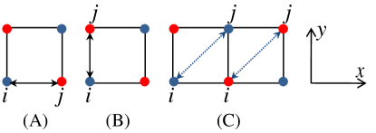
Figure 7: (Color online) Schematic illustration of four spin interactions, each spin is interacted twice. (A) Nearest neighbour hopping along $x$ direction. (B) Nearest neighbour hopping along $y$ direction. (C) Next nearest neighbour hopping.

The fourth and fifth terms in (77) are about four spin interaction with four spins located at the four lattice sites $(i,j,k,l)$ of a plaquette, see Fig.6. When spinons hop along the nearest neighbour bond in anticlockwise direction depicted in Fig.6(A), a phase $\phi_{0}$ will be acquired, then it will give rise to a flux $\phi_{ijkl}=4\phi_{0}$ across each square plaquette. It is obvious that $\phi_{ijkl}=\pi$ if $\phi_{0}=\frac{\pi}{4}$. So the spinons experience a uniform U($1$) gauge field with the magnetic flux through each plaquette being $\pi$ Wen et al. (1989). In addition to hopping in anticlockwise direction, we should consider nearest neighbour hopping in clockwise direction to get the fourth term in (77). However, the hopping events of spinons illustrated in Fig.6(B) do not carry phase because the hopping is along next nearest neighbour bond. Such hopping events lead to the fifth term in (77).

The four terms in the last line of (77) are also for four spin interactions. Different from those described above, they happen at two or three lattice sites. The first two terms correspond to four spin interactions at two neighbour sites, in which each site is interacted twice, see Fig.7. While the last two terms correspond to four spin interactions at three sites of a minimum triangular. Among the three sites, one site is interacted twice, the other two sites are interacted only once, see Fig.8.

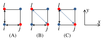
Figure 8: (Color online) Schematic illustration of four spin interactions, (A)spin at site $i$ is interacted twice; (B) spin at site $j$ is interacted twice; (C)spin at site $l$ is interacted twice.

We still use trial mean-field parameters introduced in Ref.Liu et al. (2016) to study different quantum phases. The anyonic spinons $\hat{f}_{i}=(\hat{f}_{i\uparrow},\hat{f}_{i\downarrow})^{T}$ and three Pauli matrices $\bm{\sigma}=(\sigma_{x},\sigma_{y},\sigma_{z})$ can be used to represent the spin operator at $i$th site as $\mathbb{S}_{i}=\hat{f}_{i}^{\dagger}{\bm{\sigma}\over 2}\hat{f}_{i}$ under the particle number constraint $\hat{f}_{i}^{\dagger}\hat{f}_{i}=1$.

At first, the system is assumed to have CSL phase, so the mean-field parameters about hopping can be uesd to decouple the spin interactions:

$$\chi_{1} = \langle\hat{\chi}_{ii+1_{x}}\rangle^{*}|_{i_{x}={\rm odd},i_{y}={\rm odd}}=-\langle\hat{\chi}_{ii+1_{x}}\rangle|_{i_{x}={\rm even},i_{y}={\rm odd}}$$

$$= \langle\hat{\chi}_{ii+1_{x}}\rangle|_{i_{x}={\rm odd},i_{y}={\rm even}}=-\langle\hat{\chi}_{ii+1_{x}}\rangle^{*}|_{i_{x}={\rm even},i_{y}={\rm even}}$$

$$= \langle\hat{\chi}_{ii+1_{y}}\rangle|_{i_{x}={\rm odd},i_{y}={\rm odd}}=-\langle\hat{\chi}_{ii+1_{y}}\rangle^{*}|_{i_{x}={\rm odd},i_{y}={\rm even}}$$

$$= \langle\hat{\chi}_{ii+1_{y}}\rangle^{*}|_{i_{x}={\rm even},i_{y}={\rm odd}}=-\langle\hat{\chi}_{ii+1_{y}}\rangle|_{i_{x}={\rm even},i_{y}={\rm even}},$$

$$\chi_{2} = \langle\hat{\chi}_{ii+1_{x}+1_{y}}\rangle=\chi_{2}^{*}$$ (78)

with spinon hopping operator $\hat{\chi}_{ij}=\hat{\chi}_{ji}^{\dagger}=\hat{f}_{i}^{\dagger}\hat{f}_{j}$, $i_{x}=\frac{x_{i}}{a}$ and $i_{y}=\frac{y_{i}}{a}$. Here $\chi_{2}$ is assumed to be real and the hopping phase is only carried by $\chi_{1}$ for the CSL.

Furthermore, since the system may contain symmetry breaking orders at some parameter region, we need to use the following magnetic order parameters to describe the Neel order and stripe order, respectively

$$M_{n}=(-1)^{i_{x}+i_{y}}\langle S^{z}_{i}\rangle,\ M_{s}=(-1)^{i_{x}}\langle S^{z}_{i}\rangle.$$ (79)

Now we can decouple the spin interactions by these trial mean-field parameters. The calculation is explicitly given in appendix B.

After decoupling the effective spin Hamiltonian (77) in terms of mean-field parameters $\chi_{1}$, $\chi_{2}$, $M_{n}$ and $M_{s}$, we obtain the matrix form of the Hamiltonian in real (coordinate) space. If the lattice system under investigation has $N=L_{x}\times L_{y}$ lattice sites, the Hamiltonian is a $2N\times 2N$ matrix. In calculation we use $N=16^{2}$. To minimize the free energy at $T=0$ with respect to the mean-field parameters $\chi_{1}$, $\chi_{2}$, $M_{n}$ and $M_{s}$, we may determine the phase boundary between the magnetic and CSL state.

The CSL phase in the effective Hamiltonian up to the three spin interactions has already been investigated ( see Fig.4(b) in Ref.Liu et al. (2016)). However, compared with the lower boundary $U_{c_{1}}$ of Fig.5 , the phase boundary $U_{c}$ between the CSL and magnetic order is less than $U_{c_{1}}$ when $0.05\leq t_{1}<0.55$ or $0.85<t_{1}\leq 1$ . In other words, the CSL can only appear when $0.55\leq t_{1}\leq 0.85$. So, the four spin interactions should be included to get broader $t_{1}$ region for CSL.

In the mean-field decoupling of the fourth term in (77)

$$-\{80[(\mathbf{S}_{i}\cdot\mathbf{S}_{j})(\mathbf{S}_{k}\cdot\mathbf{S}_{l})+(\mathbf{S}_{i}\cdot\mathbf{S}_{l})(\mathbf{S}_{j}\cdot\mathbf{S}_{k})$$ (80)

$$-(\mathbf{S}_{i}\cdot\mathbf{S}_{k})(\mathbf{S}_{j}\cdot\mathbf{S}_{l})]-4(\mathbf{S}_{i}\cdot\mathbf{S}_{j}+\mathbf{S}_{k}\cdot\mathbf{S}_{l}+\mathbf{S}_{j}\cdot\mathbf{S}_{k}$$

$$+\mathbf{S}_{i}\cdot\mathbf{S}_{l}+\mathbf{S}_{i}\cdot\mathbf{S}_{k}+\mathbf{S}_{j}\cdot\mathbf{S}_{l})\}$$

$$= 5[\frac{4|\chi_{1}|^{4}e^{-i\pi}}{\langle\hat{\chi}_{li}\rangle}\hat{\chi}_{li}+{\rm cyclic}(ijkl)-12|\chi_{1}|^{4}e^{-i\pi}+{\rm H.c.}]$$

$$-80[(-1)^{i_{x}+i_{y}}(M_{n}^{3}S^{z}_{i}-M_{n}^{3}S^{z}_{j}+M_{n}^{3}S^{z}_{k}-M_{n}^{3}S^{z}_{l})$$

$$-3M_{n}^{4}]-4(-1)^{i_{x}+i_{y}}(M_{n}S^{z}_{i}-M_{n}S^{z}_{j}+M_{n}S^{z}_{k}$$

$$-M_{n}S^{z}_{l})+8M_{n}^{2},$$

here $j=i+1_{x},k=i+1_{x}+1_{y},l=i+1_{y}$, even if there is a $\pi$ flux in the hopping part, this term will reduce the value of phase boundary $U_{c}$ obtained in Ref.Liu et al. (2016)) due to the $-80$ and $-4$ coefficients in the Neel order term. Therefore, in addition to (80), the other four spin interaction terms in (77) are also very important for getting reasonable phase boundary.

In Fig.9, the CSL phase does appear at some parameter region: $\chi_{1}\neq 0$, $\chi_{2}\neq 0$, but $M_{n}=M_{s}=0$. With $t_{1}$ increasing in the region $0.05\leq t_{1}\leq 0.711$, the critical Hubbard interaction strength to reach the Neel order increases . However, the critical Hubbard interaction strength to reach the stripe order decreases with $t_{1}$ increasing from $0.711$ to $1$. At $t_{1}=0.711$ the system becomes most frustrated (green point in Fig.9).

Even if these four spin interaction terms do not break time-reversal symmetry of the system, they do have qualitative effect on the CSL phase diagram of effective Hamiltonian including only two and three spin interactions in Ref.Liu et al. (2016). As in Fig.9 we can see that the CSL phase is obtained in a broader region with $0.05\leq t_{1}\leq 1$. The result is consistent with the phase diagram obtained in slave-rotor theory. We note that more accurate phase diagram can be obtained if all the four spin interaction terms are taken into account, but it has only quantitative modification over the current phase diagram.

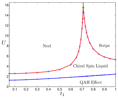
Figure 9: (Color online) Spinon mean-field phase diagram ($t_{0}=1$) based on the effective spin model, in which the relevant four spin interactions are considered.

VIII Conclusion and Discussion

In this work, we have used two different mean-field approaches to investigate the CSL phase in optical Raman lattice with $\mathrm{U}(1)$ synthetic gauge flux. At first, we determine the phase boundary of CSL based on slave-rotor theory, which is applicable in intermediate to strong Hubbard interacting regime. When the Mott transition of charge takes place, the CSL phase appears. The spinon is separated from the charge, and the band structure of spinon is very similar to that of spin-$\frac{1}{2}$ two-copy version of QAH model with gapped bulk state and chiral gapless edge state. As a disordered phase without long-range spin order, the CSL preserves spin-rotational symmetry. Therefore no magnetic orders exist in the CSL, and the Mott insulator is a nonmagnetic insulator.

When Hubbard interaction strength $U$ is strong, we manage to show CSL by spinon mean-field calculation based on an effective spin model derived from the Hubbard model and including not only two and three spin interaction terms, but also relevant four spin interaction terms. Our numerical results show that the CSL phase can be stabilized at strong magnetic frustrated system.

While the critical Hubbard interaction strength of CSL depends on the mean-field approximation methods, the phase diagrams obtained from the two different methods are consistent with each other, showing the clear numerical evidence of the CSL phase obtained for cold fermions loaded to optical Raman lattice which is of experimental feasibility. The mean-field approaches can be used to study other exotic topological phases for cold atoms of higher orbital bands and $3$D lattice systems.

Appendix A slave rotor mean field formalism

In this appendix we show some detailed calculation about the slave rotor mean field approximation. At first we discuss the transition from QAH to CSL. For the spinon Hamiltonian (49), we may get a unitary transformation between the sublattice bases $(\hat{f}_{\mathbb{k}\sigma}^{a},\hat{f}_{\mathbb{k}\sigma}^{b})$ and band bases $(\hat{f}_{\mathbb{k}\sigma}^{l},\hat{f}_{\mathbb{k}\sigma}^{u})$

$$\left(\begin{array}[]{c}\hat{f}_{\mathbb{k}\sigma}^{a}\\[5.0pt] \hat{f}_{\mathbb{k}\sigma}^{b}\end{array}\right)=\left(\begin{array}[]{cc}\alpha_{-}&\alpha_{+}\\[5.0pt] \beta_{-}&\beta_{+}\end{array}\right)\left(\begin{array}[]{c}\hat{f}_{\mathbb{k}\sigma}^{l}\\[5.0pt] \hat{f}_{\mathbb{k}\sigma}^{u}\end{array}\right).$$ (81)

By using the Fourier transformations:

$$X_{i}(\tau) = \frac{1}{\sqrt{N}}\sum_{\mathbb{k}}e^{i\mathbb{k}\cdot\mathbb{r}_{i}}X_{\mathbb{k}}(\tau),$$ (82)

$$X_{\mathbb{k}}(\tau) = \frac{1}{\sqrt{\beta}}\sum_{n}e^{-i\nu_{n}\tau}X_{\mathbb{k}}(\nu_{n}),$$ (83)

we find the first self-consistency equation from the constraint (37)

$$1 = \frac{1}{N}\sum_{\mathbb{k}}\frac{1}{\beta}\sum_{n}G_{X}(\mathbb{k},\nu_{n})$$ (84)

$$= \frac{\sqrt{2}U}{N}\sum_{\mathbb{k}}\frac{1}{\sqrt{\Delta_{X}^{2}+4U[\xi_{\mathbb{k}}-\min(\xi_{\mathbb{k}})]}}$$

In Eq. (84) we perform the Matsubara sum on Green function (53) at zero temperature (see Appendix D of Rachel and Le Hur (2010)) and introduce the insulating gap of rotor

$$\Delta_{X}=2\sqrt{U[\rho+\min{(\xi_{\mathbb{k}})}]}\ .$$ (85)

The explicit form of insulating gap $\Delta_{X}$ should be determined by $\xi_{\mathbb{k}}$ and hence by $Q_{X}$ and $Q_{X}^{\prime}$. The two mean-field parameters $Q_{X}$ and $Q_{X}^{\prime}$ are the second and third self-consistency equations, respectively. They can be determined by using unitary transformation (81).

We start with $Q_{X}$:

$$\sum_{i=1}^{4}\langle\sum_{\sigma}t_{ij}e^{i\phi_{ij}}\hat{f}_{i\sigma}^{b{\dagger}}\hat{f}_{j\sigma}^{a}\rangle$$ (86)

$$= -\frac{1}{N}\sum_{\mathbb{k}\sigma}(d_{x}+id_{y})\langle\hat{f}_{\mathbb{k}\sigma}^{b{\dagger}}\hat{f}_{\mathbb{k}\sigma}^{a}\rangle$$

$$= -\frac{1}{N}\sum_{\mathbb{k}}2(d_{x}+id_{y})\beta_{-}^{\ast}\alpha_{-}\langle\hat{f}^{l\dagger}_{\mathbb{k}\sigma}\hat{f}^{l}_{\mathbb{k}\sigma}\rangle$$

$$= -\frac{2}{N}\sum_{\mathbb{k}}(d_{x}+id_{y})\beta_{-}^{\ast}\alpha_{-},$$

where we assume $\langle\hat{f}^{l\dagger}_{\mathbb{k}\sigma}\hat{f}^{l}_{\mathbb{k}\sigma}\rangle=1$, $\langle\hat{f}^{u\dagger}_{\mathbb{k}\sigma}\hat{f}^{u}_{\mathbb{k}\sigma}\rangle=0$ for $\sigma=\uparrow,\downarrow$ since the lower band of spinon is completely filled while the upper band is empty. Due to the lattice symmetry, the sum over the four nearest neighbor sites, $\sum_{i=1}^{4}$, just appears as a factor $4$ in the final expression. Thus we find the mean-field parameter

$$Q_{X}=-\frac{1}{2N}\sum_{\mathbb{k}}(d_{x}+id_{y})\beta_{-}^{\ast}\alpha_{-}.$$ (87)

Similarly,

$$\sum_{i=1}^{4}\langle\sum_{\sigma}t_{1}\hat{f}_{i\sigma}^{\dagger}\hat{f}_{j\sigma}\rangle$$ (88)

$$= \frac{1}{2N}\sum_{\mathbb{k}\sigma}(-d_{z}\langle\hat{f}_{\mathbb{k}\sigma}^{a{\dagger}}\hat{f}_{\mathbb{k}\sigma}^{a}\rangle+d_{z}\langle\hat{f}_{\mathbb{k}\sigma}^{b{\dagger}}\hat{f}_{\mathbb{k}\sigma}^{b}\rangle)$$

$$= \frac{1}{N}\sum_{\mathbb{k}}d_{z}(-|\alpha_{-}|^{2}+|\beta_{-}|^{2})$$

Again the lattice symmetry is responsible for the fact that the sum over the four next nearest neighbor sites, $\sum_{i=1}^{4}$, can be replaced by a factor $4$

$$Q_{X}^{\prime}=\frac{1}{4N}\sum_{\mathbb{k}}d_{z}(-|\alpha_{-}|^{2}+|\beta_{-}|^{2}).$$ (89)

The rotor spectrum $\xi_{\mathbb{k}}$ of Eq. (54) is well defined and we can solve Eq. (84). If the phase transition from the Mott insulator to the superfluid of the rotor takes place, the rotor gap $\Delta_{X}$ must close. It indicates that

$$U_{c_{1}}(t_{1})=\frac{1}{2}\left[\frac{1}{2N}\sum_{\mathbb{k}^{\prime}}\frac{1}{\sqrt{\xi_{\mathbb{k}}-\min(\xi_{\mathbb{k}})}}\right]^{-2}\ ,$$ (90)

which defines the critical interaction strength of Mott insulator, i.e when $U\leq U_{c_{1}},\Delta_{X}=0$; $U>U_{c_{1}},\Delta_{X}>0$. The sum over $\mathbb{k}^{\prime}$ means that formally the lowest bound corresponds to $\mathbb{k}\to\mathbb{k}_{\rm min}+\eta$, $\eta\ll 1$ Rachel and Le Hur (2010), and $\mathbb{k}_{\rm min}$ is wave vector associated with the minimum of $\xi_{\mathbb{k}}$. Hence, divergence in the sum can be avoided. This sum rule applies to (92) and (94).

We have to study $Q_{f}$ and $Q_{f}^{\prime}$ and their behaviors along the phase boundary $U_{c_{1}}(t_{1})$. By using Fourier transformations (82) and (83),

$$Q_{f} = \langle X_{i}^{\ast}X_{j}\rangle|_{{\rm nn.}}=\frac{1}{N}\sum_{\mathbb{k}}e^{-i\mathbb{k}\cdot\bm{\delta}_{\mu}}\langle X_{\mathbb{k}}^{b\ast}X_{\mathbb{k}}^{a}\rangle$$ (91)

$$= \frac{1}{N}\sum_{\mathbb{k}}\frac{|g_{1}|}{4}\frac{1}{\beta}\sum_{n}G_{X}(\mathbb{k},\nu_{n})$$

$$= \frac{1}{N}\sum_{\mathbb{k}}\frac{|g_{1}|}{4}\frac{\sqrt{2}U}{2\sqrt{U\left(\rho+\xi_{\mathbb{k}}\right)}}\ ,$$

here $\bm{\delta}_{\mu}$ denotes one of the four nearest neighbor vectors. Along the transition line we have $\Delta_{X}=0$ and obtain

$$Q_{f}^{c}(t_{1})=\frac{\sqrt{2U_{c_{1}}(t_{1})}}{8N}\sum_{\mathbb{k}^{\prime}}\frac{|g_{1}|}{\sqrt{\xi_{\mathbb{k}}-\min{(\xi_{\mathbb{k}})}}}\ .$$ (92)

The last self-consistency equation determines $Q_{f}^{\prime}$.

$$Q_{f}^{\prime} = \langle X_{i}^{\ast}X_{j}\rangle|_{{\rm nnn.}}$$ (93)

$$= \frac{1}{N}\sum_{\mathbb{k}}e^{-i\mathbb{k}\cdot\bm{\delta}^{\prime}_{\mu}}\langle X_{\mathbb{k}}^{(a/b)\ast}X_{\mathbb{k}}^{(a/b)}\rangle$$

$$= \frac{1}{N}\sum_{\mathbb{k}}\frac{|g_{2}|}{4}\frac{1}{\beta}\sum_{n}G_{X}(\mathbb{k},\nu_{n})$$

$$= \frac{1}{N}\sum_{\mathbb{k}}\frac{|g_{2}|}{4}\frac{\sqrt{2}U}{2\sqrt{U\left(\rho+\xi_{\mathbb{k}}\right)}}\ ,$$

with $\bm{\delta}^{\prime}_{\mu}$ being one of the four next nearest neighbor vectors. Thus we find $Q_{f}^{\prime}$ along the Mott transition,

$$Q_{f}^{\prime c}(t_{1})=\frac{\sqrt{2U_{c_{1}}(t_{1})}}{8N}\sum_{\mathbb{k}^{\prime}}\frac{|g_{2}|}{\sqrt{\xi_{\mathbb{k}}-\min{(\xi_{\mathbb{k}})}}}\ .$$ (94)

Secondly, we focus on the transition from CSL to magnetic phase. For the spinon Hamiltonian (70), the two $4\times 4$ matrices $\mathcal{H}_{\uparrow}$ and $\mathcal{H}_{\downarrow}$ are

$$\mathcal{H}_{\uparrow} = \left(\begin{array}[]{cccc}-\frac{U}{4}(m_{1}+m_{2})&2it_{0}e^{i\frac{\pi}{4}}\sin(k_{x}a)Q_{f}&-4t_{1}\cos(k_{x}a)\cos(k_{y}a)Q^{\prime}_{f}&-2it_{0}e^{-i\frac{\pi}{4}}\sin(k_{y}a)Q_{f}\\ -2it_{0}e^{-i\frac{\pi}{4}}\sin(k_{x}a)Q_{f}&\frac{U}{4}(m_{1}+m_{2})&2it_{0}e^{i\frac{\pi}{4}}\sin(k_{y}a)Q_{f}&4t_{1}\cos(k_{x}a)\cos(k_{y}a)Q^{\prime}_{f}\\ -4t_{1}\cos(k_{x}a)\cos(k_{y}a)Q^{\prime}_{f}&-2it_{0}e^{-i\frac{\pi}{4}}\sin(k_{y}a)Q_{f}&-\frac{U}{4}(m_{1}-m_{2})&2it_{0}e^{i\frac{\pi}{4}}\sin(k_{x}a)Q_{f}\\ 2it_{0}e^{i\frac{\pi}{4}}\sin(k_{y}a)Q_{f}&4t_{1}\cos(k_{x}a)\cos(k_{y}a)Q^{\prime}_{f}&-2it_{0}e^{-i\frac{\pi}{4}}\sin(k_{x}a)Q_{f}&\frac{U}{4}(m_{1}-m_{2})\end{array}\right)\ ,$$ (99)

$$\mathcal{H}_{\downarrow} = \left(\begin{array}[]{cccc}\frac{U}{4}(m_{1}+m_{2})&2it_{0}e^{i\frac{\pi}{4}}\sin(k_{x}a)Q_{f}&-4t_{1}\cos(k_{x}a)\cos(k_{y}a)Q^{\prime}_{f}&-2it_{0}e^{-i\frac{\pi}{4}}\sin(k_{y}a)Q_{f}\\ -2it_{0}e^{-i\frac{\pi}{4}}\sin(k_{x}a)Q_{f}&-\frac{U}{4}(m_{1}+m_{2})&2it_{0}e^{i\frac{\pi}{4}}\sin(k_{y}a)Q_{f}&4t_{1}\cos(k_{x}a)\cos(k_{y}a)Q^{\prime}_{f}\\ -4t_{1}\cos(k_{x}a)\cos(k_{y}a)Q^{\prime}_{f}&-2it_{0}e^{-i\frac{\pi}{4}}\sin(k_{y}a)Q_{f}&\frac{U}{4}(m_{1}-m_{2})&2it_{0}e^{i\frac{\pi}{4}}\sin(k_{x}a)Q_{f}\\ 2it_{0}e^{i\frac{\pi}{4}}\sin(k_{y}a)Q_{f}&4t_{1}\cos(k_{x}a)\cos(k_{y}a)Q^{\prime}_{f}&-2it_{0}e^{-i\frac{\pi}{4}}\sin(k_{x}a)Q_{f}&-\frac{U}{4}(m_{1}-m_{2})\end{array}\right)\ .$$ (105)

The unitary transformation between the sublattice bases $(\hat{f}^{a}_{\mathbb{k}\sigma},\hat{f}^{b}_{\mathbb{k}\sigma},\hat{f}^{c}_{\mathbb{k}\sigma},\hat{f}^{d}_{\mathbb{k}\sigma})$ and band bases $(\hat{f}^{l_{1}}_{\mathbb{k}\sigma},\hat{f}^{l_{2}}_{\mathbb{k}\sigma},\hat{f}^{u_{1}}_{\mathbb{k}\sigma},\hat{f}^{u_{2}}_{\mathbb{k}\sigma})$ can be obtained

$$\left(\begin{array}[]{c}\hat{f}^{a}_{\mathbb{k}\sigma}\\[5.0pt] \hat{f}^{b}_{\mathbb{k}\sigma}\\[5.0pt] \hat{f}^{c}_{\mathbb{k}\sigma}\\[5.0pt] \hat{f}^{d}_{\mathbb{k}\sigma}\end{array}\right)=\left(\begin{array}[]{cccc}\alpha^{1}_{\sigma-}&\alpha^{2}_{\sigma-}&\alpha^{1}_{\sigma+}&\alpha^{2}_{\sigma+}\\[5.0pt] \beta^{1}_{\sigma-}&\beta^{2}_{\sigma-}&\beta^{1}_{\sigma+}&\beta^{2}_{\sigma+}\\[5.0pt] \gamma^{1}_{\sigma-}&\gamma^{2}_{\sigma-}&\gamma^{1}_{\sigma+}&\gamma^{2}_{\sigma+}\\[5.0pt] \delta^{1}_{\sigma-}&\delta^{2}_{\sigma-}&\delta^{1}_{\sigma+}&\delta^{2}_{\sigma+}\end{array}\right)\left(\begin{array}[]{c}\hat{f}^{l_{1}}_{\mathbb{k}\sigma}\\[5.0pt] \hat{f}^{l_{2}}_{\mathbb{k}\sigma}\\[5.0pt] \hat{f}^{u_{1}}_{\mathbb{k}\sigma}\\[5.0pt] \hat{f}^{u_{2}}_{\mathbb{k}\sigma}\end{array}\right).$$ (107)

The energy extreme conditions $\frac{\partial\mathcal{F}}{\partial m_{1}}=\frac{\partial\mathcal{F}}{\partial m_{2}}=0$ give the critical interaction strength $U_{c_{2}}$ of magnetic order.

The mean-field parameters $Q_{X_{1}}$, $Q_{X_{2}}$ and $Q_{X}^{\prime}$ along the phase boundary $U_{c_{2}}$ can be calculated by using the unitary transformation (107):

$$Q_{X_{1}} = \frac{1}{2N_{0}}\sum_{\mathbb{k}\in\,{\rm RBZ},\sigma}t_{0}e^{i\frac{\pi}{4}}\sin(k_{x}a)$$

$$\cdot(\beta_{\sigma-}^{1\ast}\alpha_{\sigma-}^{1}+\beta_{\sigma-}^{2\ast}\alpha_{\sigma-}^{2}+\delta_{\sigma-}^{1\ast}\gamma_{\sigma-}^{1}+\delta_{\sigma-}^{2\ast}\gamma_{\sigma-}^{2}),$$

$$Q_{X_{2}} = \frac{1}{2N_{0}}\sum_{\mathbb{k}\in\,{\rm RBZ},\sigma}t_{0}e^{-i\frac{\pi}{4}}\sin(k_{y}a)$$

$$\cdot(\delta_{\sigma-}^{1\ast}\alpha_{\sigma-}^{1}+\delta_{\sigma-}^{2\ast}\alpha_{\sigma-}^{2}+\beta_{\sigma-}^{1\ast}\gamma_{\sigma-}^{1}+\beta_{\sigma-}^{2\ast}\gamma_{\sigma-}^{2}),$$

here for the lattice symmetry, the factor $2$ in the denominator denotes two nearest neighbour sites.

$$Q_{X}^{\prime} = \langle\sum_{\sigma}t_{1}\hat{f}_{i\sigma}^{\dagger}\hat{f}_{j\sigma}\rangle$$

$$= \frac{1}{4N_{0}}\sum_{\mathbb{k}\in\,{\rm RBZ},\sigma}2t_{1}\cos(k_{x}a)\cos(k_{y}a)$$

$$\cdot(\alpha_{\sigma-}^{1\ast}\gamma_{\sigma-}^{1}+\alpha_{\sigma-}^{2\ast}\gamma_{\sigma-}^{2}-\beta_{\sigma-}^{1\ast}\delta_{\sigma-}^{1}-\beta_{\sigma-}^{2\ast}\delta_{\sigma-}^{2}),$$

here for the lattice symmetry, the factor $4$ in the denominator denotes four next nearest neighbour sites. And $\langle\hat{f}^{l_{1}\dagger}_{\mathbb{k}\sigma}\hat{f}^{l_{1}}_{\mathbb{k}\sigma}\rangle=\langle\hat{f}^{l_{2}\dagger}_{\mathbb{k}\sigma}\hat{f}^{l_{2}}_{\mathbb{k}\sigma}\rangle=1$, $\langle\hat{f}^{u_{1}\dagger}_{\mathbb{k}\sigma}\hat{f}^{u_{1}}_{\mathbb{k}\sigma}\rangle=\langle\hat{f}^{u_{2}\dagger}_{\mathbb{k}\sigma}\hat{f}^{u_{2}}_{\mathbb{k}\sigma}\rangle=0$ for $\sigma=\uparrow,\downarrow$ since the lower band is completely filled while the upper band is empty.

The self-consistency equation along the phase boundary $U_{c_{2}}$ corresponding to the constraint (37)

$$1=\frac{\sqrt{2U_{c_{2}}}}{2N}\sum_{\mathbb{k}}\frac{1}{\sqrt{\rho+\xi_{\mathbb{k}}}}.$$ (111)

determines Lagrange multiplier $\rho_{c}$ along the phase boundary $U_{c_{2}}$. Now we find the mean-field parameters $Q_{f}$ and $Q_{f}^{\prime}$ along the transition line $U_{c_{2}}$,

$$Q_{f}^{c}=\frac{\sqrt{2U_{c_{2}}}}{8N}\sum_{\mathbb{k}}\frac{|g_{1}|}{\sqrt{\xi_{\mathbb{k}}+\rho_{c}}}\ ,$$ (112)

$$Q_{f}^{\prime c}=\frac{\sqrt{2U_{c_{2}}}}{8N}\sum_{\mathbb{k}}\frac{|g_{2}|}{\sqrt{\xi_{\mathbb{k}}+\rho_{c}}}\ ,$$ (113)

here $g_{1}(\mathbb{k})=\sum_{i=1}^{4}e^{-i\mathbb{k}\cdot\bm{\delta}_{i}}$, $g_{2}(\mathbb{k})=\sum_{i=1}^{4}e^{-i\mathbb{k}\cdot\bm{\delta}_{i}^{\prime}}$.

Appendix B effective spin model

In this appendix we will briefly present the derivation of effective spin Hamiltonian and how to decouple the spin interaction terms by trial mean-field parameters. We follow the procedure in MacDonald et al. (1988) and only give the corrections up to the fourth order. As for the fourth order terms, only the terms which have important physical meaning are considered. In other words, these fourth order terms can give qualitative modification on the mean-field phase diagram obtained from the effective spin Hamiltonian which has only expansions up to the third order Liu et al. (2016).

Let’s start from the total Hamiltonian

$$H = H_{0}+H_{\rm int}$$ (114)

$$= -\sum_{\langle ij\rangle\sigma}t_{ij}e^{i\phi_{ij}}\hat{c}_{i\sigma}^{\dagger}\hat{c}_{j\sigma}-\sum_{\langle\langle ij\rangle\rangle}\sum_{\sigma}t_{1}\hat{c}_{i\sigma}^{\dagger}\hat{c}_{j\sigma}$$

$$+U\sum_{i}n_{i\uparrow}n_{i\downarrow}.$$

An effective spin model can be derived by considering the perturbation expansions about $\frac{t_{0}}{U}$, $\frac{t_{1}}{U}$, with $t_{0},t_{1}$ being small compared with $U$ at half-filled case.

By multiplying hopping term $H_{0}$ from the left by $1=n_{i\bar{\sigma}}+h_{i\bar{\sigma}}$ and from the right by $1=n_{j\bar{\sigma}}+h_{j\bar{\sigma}}$, we may rewrite Hamiltonian (114) in the following form

$$H = T_{0}+H_{\rm int}+T_{+}+T_{-},$$

$$T_{0} = -\sum_{\langle ij\rangle\sigma}t_{ij}e^{i\phi_{ij}}(h_{i\bar{\sigma}}\hat{c}^{\dagger}_{i\sigma}\hat{c}_{j\sigma}h_{j\bar{\sigma}}+n_{i\bar{\sigma}}\hat{c}^{\dagger}_{i\sigma}\hat{c}_{j\sigma}n_{j\bar{\sigma}})$$

$$-\sum_{\langle\langle ij\rangle\rangle}\sum_{\sigma}t_{1}(h_{i\bar{\sigma}}\hat{c}^{\dagger}_{i\sigma}\hat{c}_{j\sigma}h_{j\bar{\sigma}}+n_{i\bar{\sigma}}\hat{c}^{\dagger}_{i\sigma}\hat{c}_{j\sigma}n_{j\bar{\sigma}}),$$

$$T_{+} = -\sum_{\langle ij\rangle\sigma}t_{ij}e^{i\phi_{ij}}n_{i\bar{\sigma}}\hat{c}^{\dagger}_{i\sigma}\hat{c}_{j\sigma}h_{j\bar{\sigma}}$$ (116)

$$-\sum_{\langle\langle ij\rangle\rangle}\sum_{\sigma}t_{1}n_{i\bar{\sigma}}\hat{c}^{\dagger}_{i\sigma}\hat{c}_{j\sigma}h_{j\bar{\sigma}},$$

$$T_{-} = -\sum_{\langle ij\rangle\sigma}t_{ij}e^{i\phi_{ij}}h_{i\bar{\sigma}}\hat{c}^{\dagger}_{i\sigma}\hat{c}_{j\sigma}n_{j\bar{\sigma}}$$ (117)

$$-\sum_{\langle\langle ij\rangle\rangle}\sum_{\sigma}t_{1}h_{i\bar{\sigma}}\hat{c}^{\dagger}_{i\sigma}\hat{c}_{j\sigma}n_{j\bar{\sigma}},$$

where the spin indices $\sigma=\uparrow,\downarrow$, $\bar{\sigma}$ is up for $\sigma$ down and down for $\sigma$ up, $n_{i\sigma}=\hat{c}^{\dagger}_{i\sigma}\hat{c}_{i\sigma}$ and $h_{i\sigma}=1-n_{i\sigma}$. $T_{+}$ describes the process of increasing one doubly-occupied site, $T_{-}$ describes the process of decreasing one doubly-occupied site and $T_{0}$ leaves the number of doubly-occupied sites unchanged.

The effective Hamiltonian can be obtained by a canonical transformation MacDonald et al. (1988):

$$H_{\rm eff} = e^{S}He^{-S}$$ (118)

$$= H+[S,H]+\frac{1}{2}[S,[S,H]]+\frac{1}{3!}[S,[S,[S,H]]]$$

$$+\frac{1}{4!}[S,[S,[S,[S,H]]]]+\cdots.$$

In the effective Hamiltonian the hopping events which increase or decrease doubly-occupied sites must be prohibited since the ground state of the system has no doubly-occupied sites. By using commutation relations $[T_{\pm},H_{\rm int}]=\mp UT_{\pm}$, $[T_{0},H_{\rm int}]=0$, we can get the effective Hamiltonian up to the fourth order correctionsMacDonald et al. (1988):

$$H_{\rm eff} = -\frac{1}{U}T_{-}T_{+}+\frac{1}{U^{2}}T_{-}T_{0}T_{+}-\frac{1}{U^{3}}T_{-}T_{0}T_{0}T_{+}$$ (119)

$$+\frac{1}{U^{3}}T_{-}T_{+}T_{-}T_{+}-\frac{1}{2U^{3}}T_{-}T_{-}T_{+}T_{+}.$$

If all spin configurations at half-filled case are taken into account, we can reach the following effective Hamiltonian for the spin degree of freedom

$$H_{\rm eff} = \sum_{\langle ij\rangle}\frac{4t_{0}^{2}}{U}\mathbf{S}_{i}\cdot\mathbf{S}_{j}+\sum_{\langle\langle ij\rangle\rangle}\frac{4t_{1}^{2}}{U}\mathbf{S}_{i}\cdot\mathbf{S}_{j}+\sum_{ijk\in\bigtriangleup}\frac{24t_{0}^{2}t_{1}}{U^{2}}\sin(\phi_{ijk})\mathbf{S}_{i}\cdot(\mathbf{S}_{j}\times\mathbf{S}_{k})$$ (120)

$$+\frac{t_{0}^{4}}{U^{3}}\sum_{ijkl\in\Box}\cos(\phi_{ijkl})\{80[(\mathbf{S}_{i}\cdot\mathbf{S}_{j})(\mathbf{S}_{k}\cdot\mathbf{S}_{l})+(\mathbf{S}_{i}\cdot\mathbf{S}_{l})(\mathbf{S}_{j}\cdot\mathbf{S}_{k})-(\mathbf{S}_{i}\cdot\mathbf{S}_{k})(\mathbf{S}_{j}\cdot\mathbf{S}_{l})]$$

$$-4(\mathbf{S}_{i}\cdot\mathbf{S}_{j}+\mathbf{S}_{k}\cdot\mathbf{S}_{l}+\mathbf{S}_{j}\cdot\mathbf{S}_{k}+\mathbf{S}_{i}\cdot\mathbf{S}_{l}+\mathbf{S}_{i}\cdot\mathbf{S}_{k}+\mathbf{S}_{j}\cdot\mathbf{S}_{l})\}$$

$$+\frac{t_{1}^{4}}{U^{3}}\sum_{ijkl\in\diamond}\{80[(\mathbf{S}_{i}\cdot\mathbf{S}_{j})(\mathbf{S}_{k}\cdot\mathbf{S}_{l})+(\mathbf{S}_{i}\cdot\mathbf{S}_{l})(\mathbf{S}_{j}\cdot\mathbf{S}_{k})-(\mathbf{S}_{i}\cdot\mathbf{S}_{k})(\mathbf{S}_{j}\cdot\mathbf{S}_{l})]$$

$$-4(\mathbf{S}_{i}\cdot\mathbf{S}_{j}+\mathbf{S}_{k}\cdot\mathbf{S}_{l}+\mathbf{S}_{j}\cdot\mathbf{S}_{k}+\mathbf{S}_{i}\cdot\mathbf{S}_{l}+\mathbf{S}_{i}\cdot\mathbf{S}_{k}+\mathbf{S}_{j}\cdot\mathbf{S}_{l})\}$$

$$-\frac{16t_{0}^{4}}{U^{3}}\sum_{\langle ij\rangle}\mathbf{S}_{i}\cdot\mathbf{S}_{j}-\frac{16t_{1}^{4}}{U^{3}}\sum_{\langle\langle ij\rangle\rangle}\mathbf{S}_{i}\cdot\mathbf{S}_{j}+\frac{16t_{0}^{2}t_{1}^{2}}{U^{3}}\sum_{\langle ij\rangle}\mathbf{S}_{i}\cdot\mathbf{S}_{j}+\frac{8t_{0}^{4}}{U^{3}}\sum_{\langle\langle ij\rangle\rangle}\mathbf{S}_{i}\cdot\mathbf{S}_{j},$$

where the spin operators at $i$th site are defined as: $S^{x}_{i}=\frac{1}{2}(\hat{c}^{{\dagger}}_{i\downarrow}\hat{c}_{i\uparrow}+\hat{c}^{{\dagger}}_{i\uparrow}\hat{c}_{i\downarrow})$, $S^{y}_{i}=\frac{i}{2}(\hat{c}^{{\dagger}}_{i\downarrow}\hat{c}_{i\uparrow}-\hat{c}^{{\dagger}}_{i\uparrow}\hat{c}_{i\downarrow})$, $S^{z}_{i}=\frac{1}{2}(\hat{c}^{{\dagger}}_{i\uparrow}\hat{c}_{i\uparrow}-\hat{c}^{{\dagger}}_{i\downarrow}\hat{c}_{i\downarrow})$.

Obviously, the time-reversal symmetry of system is broken due to the appearance of the third term. The summation in the third term means that each set of $(i,j,k)$ consists of a minimum triangular. $\phi_{ijk}$ is the Aharonov-Bohm phase acquired by hopping through the closed minimum triangular loop in anticlockwise direction $i\rightarrow j\rightarrow k\rightarrow i$. It can be verified that $\phi_{ijk}=\frac{\pi}{2}$ when $\phi_{0}=\frac{\pi}{4}$.

To study different phases we should introduce mean-field parameters. At first we use the anyonic spinons $\hat{f}_{i}=(\hat{f}_{i\uparrow},\hat{f}_{i\downarrow})^{T}$ to represent the spin operator as $\mathbb{S}_{i}=\hat{f}_{i}^{\dagger}{\bm{\sigma}\over 2}\hat{f}_{i}$ as long as the particle number $\hat{f}_{i}^{\dagger}\hat{f}_{i}=1$ at each site, where $\bm{\sigma}=(\sigma_{x},\sigma_{y},\sigma_{z})$. The two and three spin interaction terms can be rewritten as the following by using the spinon hopping operator $\hat{\chi}_{ij}=\hat{\chi}_{ji}^{\dagger}=\hat{f}_{i}^{\dagger}\hat{f}_{j}$,

$$\mathbb{S}_{i}\cdot\mathbb{S}_{j} = -{1\over 2}\hat{\chi}_{ij}\hat{\chi}_{ji},$$ (121)

$$\mathbf{S}_{i}\cdot(\mathbf{S}_{j}\times\mathbf{S}_{k}) = {1\over 24i}\{[\hat{\chi}_{ij}\hat{\chi}_{jk}\hat{\chi}_{ki}+\hat{\chi}_{jk}\hat{\chi}_{ij}\hat{\chi}_{ki}$$ (122)

$$+{\rm cyclic}(ijk)]-{\rm H.c.}\}.$$

In general the spinon hopping term is complex, and the spin chirality term can give rise to a phase $e^{i\phi_{\Delta}}$, with the flux $\phi_{\Delta}={\rm Arg}(\langle\hat{\chi}_{ik}\rangle\langle\hat{\chi}_{kj}\rangle\langle\hat{\chi}_{ji}\rangle)$ experienced by spinons after hopping through a closed minimum triangular loop in anticlockwise direction $i\rightarrow j\rightarrow k\rightarrow i$. When $\phi_{\Delta}=\frac{\pi}{2}$ the spinons experience a uniform U($1$) gauge field, with the magnetic flux through each triangular being $\frac{\pi}{2}$ and through each plaquette being $\pi$ Wen et al. (1989).

The mean-field parameters about hopping can be introduced to decouple the spin interactions (see Eqs.(VII)):

$$\chi_{1} = \langle\hat{\chi}_{ii+1_{x}}\rangle^{*}|_{i_{x}={\rm odd},i_{y}={\rm odd}}=-\langle\hat{\chi}_{ii+1_{x}}\rangle|_{i_{x}={\rm even},i_{y}={\rm odd}}$$

$$= \langle\hat{\chi}_{ii+1_{x}}\rangle|_{i_{x}={\rm odd},i_{y}={\rm even}}=-\langle\hat{\chi}_{ii+1_{x}}\rangle^{*}|_{i_{x}={\rm even},i_{y}={\rm even}}$$

$$= \langle\hat{\chi}_{ii+1_{y}}\rangle|_{i_{x}={\rm odd},i_{y}={\rm odd}}=-\langle\hat{\chi}_{ii+1_{y}}\rangle^{*}|_{i_{x}={\rm odd},i_{y}={\rm even}}$$

$$= \langle\hat{\chi}_{ii+1_{y}}\rangle^{*}|_{i_{x}={\rm even},i_{y}={\rm odd}}=-\langle\hat{\chi}_{ii+1_{y}}\rangle|_{i_{x}={\rm even},i_{y}={\rm even}},$$

$$\chi_{2} = \langle\hat{\chi}_{ii+1_{x}+1_{y}}\rangle=\chi_{2}^{*}$$

with $i_{x}=\frac{x_{i}}{a}$, $i_{y}=\frac{y_{i}}{a}$. Here $\chi_{2}$ is assumed to be real and the hopping phase is only carried by $\chi_{1}$ for the CSL phase.

Furthermore, since the system may contain symmetry breaking orders at some parameter region, we also need to introduce the following magnetic order parameters to describe the Neel order and stripe order, respectively

$$M_{n}=(-1)^{i_{x}+i_{y}}\langle S^{z}_{i}\rangle,\ M_{s}=(-1)^{i_{x}}\langle S^{z}_{i}\rangle,$$ (123)

Now we can decouple the spin interactions by these trial mean-field parameters. The first term in (120) is interaction of two spins on nearest neighbour sites

$$\mathbf{S}_{i}\cdot\mathbf{S}_{j} = -\frac{1}{2}\langle\hat{\chi}_{ji}\rangle\hat{\chi}_{ij}+{\rm H.c.}+\frac{1}{2}|\chi_{1}|^{2}$$

$$+(-1)^{i_{x}+i_{y}}(M_{n}S^{z}_{j}-M_{n}S^{z}_{i})+M_{n}^{2},$$

here $j=i+1_{x}$ or $j=i+1_{y}$. And the second term in (120) is interaction of two spins on next nearest neighbour sites

$$\mathbf{S}_{i}\cdot\mathbf{S}_{j} = -\frac{1}{2}\langle\hat{\chi}_{ji}\rangle\hat{\chi}_{ij}+{\rm H.c.}+\frac{1}{2}|\chi_{2}|^{2}$$ (125)

$$+(-1)^{i_{x}+i_{y}}(M_{n}S^{z}_{j}+M_{n}S^{z}_{i})-M_{n}^{2}$$

$$+(-1)^{i_{x}}(M_{s}S^{z}_{j}-M_{s}S^{z}_{i})+M_{s}^{2},$$

here $j=i+1_{x}+1_{y}$.

Both the Neel order $M_{n}$ and the stripe order $M_{s}$ are collinear, so they don’t appear in decoupling the spin chirality interaction term $\mathbf{S}_{i}\cdot(\mathbf{S}_{j}\times\mathbf{S}_{k})$

$$\mathbf{S}_{i}\cdot(\mathbf{S}_{j}\times\mathbf{S}_{k})$$ (126)

$$= \frac{1}{12i}[3\langle\hat{\chi}_{ij}\hat{\chi}_{jk}\rangle\hat{\chi}_{ki}+{\rm cyclic}(ijk)-{\rm H.c.}]$$

$$-{1\over 12i}(6\langle\hat{\chi}_{ij}\rangle\langle\hat{\chi}_{jk}\rangle\langle\hat{\chi}_{ki}\rangle-{\rm H.c.})$$

$$= {1\over 12i}[3{|\chi_{1}^{2}\chi_{2}|e^{-i\phi_{\Delta}}\over\langle\hat{\chi}_{ki}\rangle}\hat{\chi}_{ki}+{\rm cyclic}(ijk)-{\rm H.c.}]$$

$$-{1\over 12i}(6|\chi_{1}^{2}\chi_{2}|e^{-i\phi_{\Delta}}-{\rm H.c.})$$

with $\chi_{1}=|\chi_{1}|e^{i\frac{\pi}{4}}$. When we determine the matrix elements of the above three spin interaction term, we should keep in mind that every square plaquette contains four minimum triangular loops and every nearest neighbour bond is shared by four minimum triangular loops, but every next nearest neighbour bond is shared by only two minimum triangular loops.

When the spinons hop through a square plaquette in the direction and opposite direction of Fig.6(A) of the main text, it will lead to the fourth part in (120). It contains only nearest neighbour hopping. $\phi_{ijkl}$ is the phase acquired by hopping through a closed square plaquette in anticlockwise direction $i\rightarrow j\rightarrow k\rightarrow l\rightarrow i$. It can be verified that $\phi_{ijkl}=\pi$ when $\phi_{0}=\frac{\pi}{4}$. The four spin interaction terms can be rewritten by the spinon hopping operator:

$$-\{80[(\mathbf{S}_{i}\cdot\mathbf{S}_{j})(\mathbf{S}_{k}\cdot\mathbf{S}_{l})+(\mathbf{S}_{i}\cdot\mathbf{S}_{l})(\mathbf{S}_{j}\cdot\mathbf{S}_{k})-(\mathbf{S}_{i}\cdot\mathbf{S}_{k})(\mathbf{S}_{j}\cdot\mathbf{S}_{l})]$$

$$-4(\mathbf{S}_{i}\cdot\mathbf{S}_{j}+\mathbf{S}_{k}\cdot\mathbf{S}_{l}+\mathbf{S}_{j}\cdot\mathbf{S}_{k}+\mathbf{S}_{i}\cdot\mathbf{S}_{l}+\mathbf{S}_{i}\cdot\mathbf{S}_{k}+\mathbf{S}_{j}\cdot\mathbf{S}_{l})\}$$

$$=\hat{\chi}_{ij}\hat{\chi}_{jk}\hat{\chi}_{kl}\hat{\chi}_{li}+\hat{\chi}_{jk}\hat{\chi}_{kl}\hat{\chi}_{ij}\hat{\chi}_{li}+\hat{\chi}_{jk}\hat{\chi}_{ij}\hat{\chi}_{kl}\hat{\chi}_{li}+\hat{\chi}_{kl}\hat{\chi}_{jk}\hat{\chi}_{ij}\hat{\chi}_{li}+\frac{1}{2}(\hat{\chi}_{ij}\hat{\chi}_{kl}\hat{\chi}_{jk}\hat{\chi}_{li}+\hat{\chi}_{kl}\hat{\chi}_{ij}\hat{\chi}_{jk}\hat{\chi}_{li})+{\rm cyclic}(ijkl)+{\rm H.c.},$$

here $j=i+1_{x},k=i+1_{x}+1_{y},l=i+1_{y}$. The four spin interaction terms can be decoupled by trial mean-field parameters as

$$-\{80[(\mathbf{S}_{i}\cdot\mathbf{S}_{j})(\mathbf{S}_{k}\cdot\mathbf{S}_{l})+(\mathbf{S}_{i}\cdot\mathbf{S}_{l})(\mathbf{S}_{j}\cdot\mathbf{S}_{k})-(\mathbf{S}_{i}\cdot\mathbf{S}_{k})(\mathbf{S}_{j}\cdot\mathbf{S}_{l})]$$

$$-4(\mathbf{S}_{i}\cdot\mathbf{S}_{j}+\mathbf{S}_{k}\cdot\mathbf{S}_{l}+\mathbf{S}_{j}\cdot\mathbf{S}_{k}+\mathbf{S}_{i}\cdot\mathbf{S}_{l}+\mathbf{S}_{i}\cdot\mathbf{S}_{k}+\mathbf{S}_{j}\cdot\mathbf{S}_{l})\}$$

$$= 5[4\langle\hat{\chi}_{ij}\rangle\langle\hat{\chi}_{jk}\rangle\langle\hat{\chi}_{kl}\rangle\hat{\chi}_{li}+{\rm cyclic}(ijkl)-12\langle\hat{\chi}_{ij}\rangle\langle\hat{\chi}_{jk}\rangle\langle\hat{\chi}_{kl}\rangle\langle\hat{\chi}_{li}\rangle+{\rm H.c.}]$$

$$-\{80[(\mathbf{S}_{i}\cdot\mathbf{S}_{j})(\mathbf{S}_{k}\cdot\mathbf{S}_{l})-(\mathbf{S}_{i}\times\mathbf{S}_{j})\cdot(\mathbf{S}_{k}\times\mathbf{S}_{l})]$$

$$-4(\mathbf{S}_{i}\cdot\mathbf{S}_{j}+\mathbf{S}_{k}\cdot\mathbf{S}_{l}+\mathbf{S}_{j}\cdot\mathbf{S}_{k}+\mathbf{S}_{i}\cdot\mathbf{S}_{l}+\mathbf{S}_{i}\cdot\mathbf{S}_{k}+\mathbf{S}_{j}\cdot\mathbf{S}_{l})\}$$

$$= 5[\frac{4|\chi_{1}|^{4}e^{-i\pi}}{\langle\hat{\chi}_{li}\rangle}\hat{\chi}_{li}+{\rm cyclic}(ijkl)-12|\chi_{1}|^{4}e^{-i\pi}+{\rm H.c.}]$$

$$-80[(-1)^{i_{x}+i_{y}}(M_{n}^{3}S^{z}_{i}-M_{n}^{3}S^{z}_{j}+M_{n}^{3}S^{z}_{k}-M_{n}^{3}S^{z}_{l})-3M_{n}^{4}]$$

$$-4(-1)^{i_{x}+i_{y}}(M_{n}S^{z}_{i}-M_{n}S^{z}_{j}+M_{n}S^{z}_{k}-M_{n}S^{z}_{l})+8M_{n}^{2}.$$

When the spinons hop through a square plaquette in the direction and opposite direction of Fig.6(B) of the main text, it will lead to the fifth part in (120). It contains only next nearest neighbour hopping. The four spin interaction terms can also be rewritten by the spinon hopping operator:

$$80[(\mathbf{S}_{i}\cdot\mathbf{S}_{j})(\mathbf{S}_{k}\cdot\mathbf{S}_{l})+(\mathbf{S}_{i}\cdot\mathbf{S}_{l})(\mathbf{S}_{j}\cdot\mathbf{S}_{k})-(\mathbf{S}_{i}\cdot\mathbf{S}_{k})(\mathbf{S}_{j}\cdot\mathbf{S}_{l})]$$

$$-4(\mathbf{S}_{i}\cdot\mathbf{S}_{j}+\mathbf{S}_{k}\cdot\mathbf{S}_{l}+\mathbf{S}_{j}\cdot\mathbf{S}_{k}+\mathbf{S}_{i}\cdot\mathbf{S}_{l}+\mathbf{S}_{i}\cdot\mathbf{S}_{k}+\mathbf{S}_{j}\cdot\mathbf{S}_{l})$$

$$=-\hat{\chi}_{ij}\hat{\chi}_{jk}\hat{\chi}_{kl}\hat{\chi}_{li}-\hat{\chi}_{jk}\hat{\chi}_{kl}\hat{\chi}_{ij}\hat{\chi}_{li}-\hat{\chi}_{jk}\hat{\chi}_{ij}\hat{\chi}_{kl}\hat{\chi}_{li}-\hat{\chi}_{kl}\hat{\chi}_{jk}\hat{\chi}_{ij}\hat{\chi}_{li}-\frac{1}{2}(\hat{\chi}_{ij}\hat{\chi}_{kl}\hat{\chi}_{jk}\hat{\chi}_{li}+\hat{\chi}_{kl}\hat{\chi}_{ij}\hat{\chi}_{jk}\hat{\chi}_{li})+{\rm cyclic}(ijkl)+{\rm H.c.},$$

here $j=i+1_{x}+1_{y},k=i+2_{y},l=i-1_{x}+1_{y}$. The four spin interaction terms can be decoupled by trial mean-field parameters as

$$80[(\mathbf{S}_{i}\cdot\mathbf{S}_{j})(\mathbf{S}_{k}\cdot\mathbf{S}_{l})+(\mathbf{S}_{i}\cdot\mathbf{S}_{l})(\mathbf{S}_{j}\cdot\mathbf{S}_{k})-(\mathbf{S}_{i}\cdot\mathbf{S}_{k})(\mathbf{S}_{j}\cdot\mathbf{S}_{l})]$$

$$-4(\mathbf{S}_{i}\cdot\mathbf{S}_{j}+\mathbf{S}_{k}\cdot\mathbf{S}_{l}+\mathbf{S}_{j}\cdot\mathbf{S}_{k}+\mathbf{S}_{i}\cdot\mathbf{S}_{l}+\mathbf{S}_{i}\cdot\mathbf{S}_{k}+\mathbf{S}_{j}\cdot\mathbf{S}_{l})$$

$$= -5[4\langle\hat{\chi}_{ij}\rangle\langle\hat{\chi}_{jk}\rangle\langle\hat{\chi}_{kl}\rangle\hat{\chi}_{li}+{\rm cyclic}(ijkl)$$

$$-12\langle\hat{\chi}_{ij}\rangle\langle\hat{\chi}_{jk}\rangle\langle\hat{\chi}_{kl}\rangle\langle\hat{\chi}_{li}\rangle+{\rm H.c.}]$$

$$+80[(\mathbf{S}_{i}\cdot\mathbf{S}_{j})(\mathbf{S}_{k}\cdot\mathbf{S}_{l})-(\mathbf{S}_{i}\times\mathbf{S}_{j})\cdot(\mathbf{S}_{k}\times\mathbf{S}_{l})]$$

$$-4(\mathbf{S}_{i}\cdot\mathbf{S}_{j}+\mathbf{S}_{k}\cdot\mathbf{S}_{l}+\mathbf{S}_{j}\cdot\mathbf{S}_{k}+\mathbf{S}_{i}\cdot\mathbf{S}_{l}+\mathbf{S}_{i}\cdot\mathbf{S}_{k}+\mathbf{S}_{j}\cdot\mathbf{S}_{l})$$

$$= -5[4\chi_{2}^{3}\hat{\chi}_{li}+{\rm cyclic}(ijkl)-12\chi_{2}^{4}+{\rm H.c.}]$$

$$+80[(-1)^{i_{x}+i_{y}}(M_{n}^{3}S^{z}_{i}+M_{n}^{3}S^{z}_{j}+M_{n}^{3}S^{z}_{k}+M_{n}^{3}S^{z}_{l})-3M_{n}^{4}]$$

$$-12(-1)^{i_{x}+i_{y}}(M_{n}S^{z}_{i}+M_{n}S^{z}_{j}+M_{n}S^{z}_{k}+M_{n}S^{z}_{l})+24M_{n}^{2}$$

$$+80[(-1)^{i_{x}}(M_{s}^{3}S^{z}_{i}-M_{s}^{3}S^{z}_{j}+M_{s}^{3}S^{z}_{k}-M_{s}^{3}S^{z}_{l})-3M_{s}^{4}]$$

$$+4(-1)^{i_{x}}(M_{s}S^{z}_{i}-M_{s}S^{z}_{j}+M_{s}S^{z}_{k}-M_{s}S^{z}_{l})-8M_{s}^{2}.$$

Note that both the Neel order $M_{n}$ and the stripe order $M_{s}$ don’t appear in decoupling the four spin interaction term $(\mathbf{S}_{i}\times\mathbf{S}_{j})\cdot(\mathbf{S}_{k}\times\mathbf{S}_{l})$ because they are collinear.

The terms about hopping events $i\leftrightarrow j,k\leftrightarrow l$ appear in the last two parts of (119): $T_{-}T_{+}T_{-}T_{+}-\frac{1}{2}T_{-}T_{-}T_{+}T_{+}$, but they are canceled by each other.

The first two terms in the last line of (120) are about interaction of two spins located at two neighbour sites in Fig.7 of the main text. Each spin is interacted twice.

Using spinon hopping operators to rewrite the spin-interaction term:

$$-16\mathbf{S}_{i}\cdot\mathbf{S}_{j}$$

$$= 2\sum_{\sigma}(\hat{\chi}_{ij}\hat{f}^{\dagger}_{j\sigma}\hat{f}_{i\sigma}\hat{f}^{\dagger}_{i\sigma}\hat{f}_{j\sigma}\hat{\chi}_{ji}+\hat{\chi}_{ji}\hat{f}^{\dagger}_{i\bar{\sigma}}\hat{f}_{j\bar{\sigma}}\hat{f}^{\dagger}_{i\sigma}\hat{f}_{j\sigma}\hat{\chi}_{ji}).$$

Under mean-field approximation,

$$\sum_{\sigma}\hat{\chi}_{ij}\hat{f}^{\dagger}_{j\sigma}\hat{f}_{i\sigma}\hat{f}^{\dagger}_{i\sigma}\hat{f}_{j\sigma}\hat{\chi}_{ji}$$

$$= \sum_{\sigma}[\langle\hat{\chi}_{ij}\rangle\langle\hat{f}^{\dagger}_{j\sigma}\hat{f}_{i\sigma}\rangle\langle\hat{f}^{\dagger}_{i\sigma}\hat{f}_{j\sigma}\rangle\hat{\chi}_{ji}$$

$$+\langle\hat{\chi}_{ij}\rangle\langle\hat{f}^{\dagger}_{j\sigma}\hat{f}_{i\sigma}\rangle\hat{f}^{\dagger}_{i\sigma}\hat{f}_{j\sigma}\langle\hat{\chi}_{ji}\rangle$$

$$+\langle\hat{\chi}_{ij}\rangle\hat{f}^{\dagger}_{j\sigma}\hat{f}_{i\sigma}\langle\hat{f}^{\dagger}_{i\sigma}\hat{f}_{j\sigma}\rangle\langle\hat{\chi}_{ji}\rangle$$

$$+\hat{\chi}_{ij}\langle\hat{f}^{\dagger}_{j\sigma}\hat{f}_{i\sigma}\rangle\langle\hat{f}^{\dagger}_{i\sigma}\hat{f}_{j\sigma}\rangle\langle\hat{\chi}_{ji}\rangle$$

$$-3\langle\hat{\chi}_{ij}\rangle\langle\hat{f}^{\dagger}_{j\sigma}\hat{f}_{i\sigma}\rangle\langle\hat{f}^{\dagger}_{i\sigma}\hat{f}_{j\sigma}\rangle\langle\hat{\chi}_{ji}\rangle]$$

$$= |\langle\hat{\chi}_{ij}\rangle|^{2}(\langle\hat{\chi}_{ij}\rangle\hat{\chi}_{ji}+\langle\hat{\chi}_{ji}\rangle\hat{\chi}_{ij})-\frac{3}{2}|\langle\hat{\chi}_{ij}\rangle|^{4},$$

$$\sum_{\sigma}\hat{\chi}_{ji}\hat{f}^{\dagger}_{i\bar{\sigma}}\hat{f}_{j\bar{\sigma}}\hat{f}^{\dagger}_{i\sigma}\hat{f}_{j\sigma}\hat{\chi}_{ji}$$

$$= |\langle\hat{\chi}_{ij}\rangle|^{2}(\langle\hat{\chi}_{ij}\rangle\hat{\chi}_{ji}+\langle\hat{\chi}_{ji}\rangle\hat{\chi}_{ij})-\frac{3}{2}|\langle\hat{\chi}_{ij}\rangle|^{4},$$

where we use $\langle\hat{f}^{\dagger}_{i\uparrow}\hat{f}_{j\uparrow}\rangle=\langle\hat{f}^{\dagger}_{i\downarrow}\hat{f}_{j\downarrow}\rangle=\frac{1}{2}\langle\hat{\chi}_{ij}\rangle$.

We can decouple the two terms by trial mean-field parameters

$$-16\mathbf{S}_{i}\cdot\mathbf{S}_{j} = 4|\chi_{1}|^{2}(\langle\hat{\chi}_{ij}\rangle\hat{\chi}_{ji}+\langle\hat{\chi}_{ji}\rangle\hat{\chi}_{ij})-6|\chi_{1}|^{4}$$

$$-16[(-1)^{i_{x}+i_{y}}(M_{n}S^{z}_{j}-M_{n}S^{z}_{i})+M_{n}^{2}],$$

here $j=i+1_{x}$ or $j=i+1_{y}$,

$$-16\mathbf{S}_{i}\cdot\mathbf{S}_{j} = 4\chi_{2}^{2}(\langle\hat{\chi}_{ij}\rangle\hat{\chi}_{ji}+\langle\hat{\chi}_{ji}\rangle\hat{\chi}_{ij})-6\chi_{2}^{4}$$

$$-16[(-1)^{i_{x}+i_{y}}(M_{n}S^{z}_{j}+M_{n}S^{z}_{i})-M_{n}^{2}]$$

$$-16[(-1)^{i_{x}}(M_{s}S^{z}_{j}-M_{s}S^{z}_{i})+M_{s}^{2}],$$

here $j=i+1_{x}+1_{y}$.

The three spins located at the three sites of minimum triangular loop also give rise to four spin interactions, in which one spin is interacted twice while the other two spins are interacted only once. They are illustrated in Fig.8 of the main text and correspond to the last two terms in the last line of (120). The two terms can be obtained by using spinon hopping operators to rewrite the spin interaction term:

$$4\mathbf{S}_{j}\cdot\mathbf{S}_{l}+{\rm cyclic}(ijl)$$ (135)

$$= \{\sum_{\sigma}(\hat{\chi}_{il}\hat{f}^{\dagger}_{l\sigma}\hat{f}_{i\sigma}\hat{f}^{\dagger}_{i\sigma}\hat{f}_{j\sigma}\hat{\chi}_{ji}+\hat{\chi}_{ij}\hat{f}^{\dagger}_{j\sigma}\hat{f}_{i\sigma}\hat{f}^{\dagger}_{l\bar{\sigma}}\hat{f}_{i\bar{\sigma}}\hat{\chi}_{il}$$

$$+\hat{\chi}_{li}\hat{f}^{\dagger}_{i\bar{\sigma}}\hat{f}_{l\bar{\sigma}}\hat{f}^{\dagger}_{i\sigma}\hat{f}_{j\sigma}\hat{\chi}_{ji}+\hat{\chi}_{ji}\hat{f}^{\dagger}_{i\sigma}\hat{f}_{j\sigma}\hat{f}^{\dagger}_{l\sigma}\hat{f}_{i\sigma}\hat{\chi}_{il}+j\leftrightarrow l)$$

$$-[(\sum_{\sigma}\hat{\chi}_{li}\hat{f}^{\dagger}_{i\sigma}\hat{f}_{j\sigma}\hat{f}^{\dagger}_{i\bar{\sigma}}\hat{f}_{l\bar{\sigma}}\hat{\chi}_{ji}+j\leftrightarrow l)+{\rm H.c.}]$$

$$-\sum_{\sigma}(\hat{\chi}_{ij}\hat{f}^{\dagger}_{l\sigma}\hat{f}_{i\sigma}\hat{f}^{\dagger}_{i\sigma}\hat{f}_{l\sigma}\hat{\chi}_{ji}+\hat{\chi}_{ji}\hat{f}^{\dagger}_{i\sigma}\hat{f}_{l\sigma}\hat{f}^{\dagger}_{l\sigma}\hat{f}_{i\sigma}\hat{\chi}_{ij}$$

$$+j\leftrightarrow l)\}+{\rm cyclic}(ijl),$$

where the term $4\mathbf{S}_{j}\cdot\mathbf{S}_{l}$ corresponds to spin interaction illustrated in Fig.8(A), which contains only nearest neighbour hopping, while the terms $4\mathbf{S}_{i}\cdot\mathbf{S}_{l}$ and $4\mathbf{S}_{i}\cdot\mathbf{S}_{j}$ in ${\rm cyclic}(ijl)$ correspond to spin interactions illustrated in Fig.8(B) and (C), which contain not only nearest neighbour hopping, but next nearest neighbour hopping. Also note that every nearest neighbour bond is shared by four minimum triangular loops, but every next nearest neighbour bond is shared by only two minimum triangular loops, we can thus obtain the last two terms of (120). When using trial mean-field parameters to decouple the spin interaction term (135), we find

$$\sum_{\sigma}(\hat{\chi}_{il}\hat{f}^{\dagger}_{l\sigma}\hat{f}_{i\sigma}\hat{f}^{\dagger}_{i\sigma}\hat{f}_{j\sigma}\hat{\chi}_{ji}+\hat{\chi}_{ij}\hat{f}^{\dagger}_{j\sigma}\hat{f}_{i\sigma}\hat{f}^{\dagger}_{l\bar{\sigma}}\hat{f}_{i\bar{\sigma}}\hat{\chi}_{il}$$ (136)

$$+\hat{\chi}_{li}\hat{f}^{\dagger}_{i\bar{\sigma}}\hat{f}_{l\bar{\sigma}}\hat{f}^{\dagger}_{i\sigma}\hat{f}_{j\sigma}\hat{\chi}_{ji}+\hat{\chi}_{ji}\hat{f}^{\dagger}_{i\sigma}\hat{f}_{j\sigma}\hat{f}^{\dagger}_{l\sigma}\hat{f}_{i\sigma}\hat{\chi}_{il}+j\leftrightarrow l)$$

$$-[(\sum_{\sigma}\hat{\chi}_{li}\hat{f}^{\dagger}_{i\sigma}\hat{f}_{j\sigma}\hat{f}^{\dagger}_{i\bar{\sigma}}\hat{f}_{l\bar{\sigma}}\hat{\chi}_{ji}+j\leftrightarrow l)+{\rm H.c.}]$$

$$-\sum_{\sigma}(\hat{\chi}_{ij}\hat{f}^{\dagger}_{l\sigma}\hat{f}_{i\sigma}\hat{f}^{\dagger}_{i\sigma}\hat{f}_{l\sigma}\hat{\chi}_{ji}+\hat{\chi}_{ji}\hat{f}^{\dagger}_{i\sigma}\hat{f}_{l\sigma}\hat{f}^{\dagger}_{l\sigma}\hat{f}_{i\sigma}\hat{\chi}_{ij}$$

$$+j\leftrightarrow l)$$

$$= [4|\langle\hat{\chi}_{ij}\rangle|^{2}(\langle\hat{\chi}_{il}\rangle\hat{\chi}_{li}+\langle\hat{\chi}_{li}\rangle\hat{\chi}_{il})+j\leftrightarrow l$$

$$-12|\langle\hat{\chi}_{ij}\rangle|^{2}|\langle\hat{\chi}_{il}\rangle|^{2}]$$

$$-[4|\langle\hat{\chi}_{ij}\rangle|^{2}(\langle\hat{\chi}_{il}\rangle\hat{\chi}_{li}+\langle\hat{\chi}_{li}\rangle\hat{\chi}_{il})+j\leftrightarrow l$$

$$-12|\langle\hat{\chi}_{ij}\rangle|^{2}|\langle\hat{\chi}_{il}\rangle|^{2}]$$

$$= 0.$$

Therefore the mean-field approximation of hopping terms is equal to zero. We can only use magnetic order parameters to decouple the last two terms of (120):

$$16\mathbf{S}_{i}\cdot\mathbf{S}_{j} = 16[(-1)^{i_{x}+i_{y}}(M_{n}S^{z}_{j}-M_{n}S^{z}_{i})+M_{n}^{2}],$$

here $j=i+1_{x}$ or $j=i+1_{y}$,

$$8\mathbf{S}_{i}\cdot\mathbf{S}_{j} = 8[(-1)^{i_{x}+i_{y}}(M_{n}S^{z}_{j}+M_{n}S^{z}_{i})-M_{n}^{2}],$$

here $j=i+1_{x}+1_{y}$.