Lithium in Kepler Red Giants: Defining Normal and Anomalous

Abstract

The orders of magnitude variation in lithium abundances of evolved stars have long been a puzzle. Diluted signals, ambiguous evolutionary states and unknown masses have made it challenging to both map the expected lithium signals and explain the anomalously lithium-rich stars. We show here using a set of asteroseismically characterized evolved stars that the base lithium abundance in red giant stars is mass dependent, with higher mass stars having higher ‘normal’ lithium abundances, while highly lithium enhanced stars may cluster around 0.8 or 1.8 M_☉. We confirm previous studies that have shown that lithium enhancement and rapid rotation are often coincident, but find that the actual correlation between lithium abundance and the rotation rate, whether surface rotation, internal rotation, or radial differential rotation, is weak. Our data support previous assertions that most lithium rich giants are in the core-helium burning phase. We also note a tentative correlation between the highest lithium abundances and unusual carbon to nitrogen ratios, which is suggestive of binary interactions, though we find no simple correlation between lithium richness and indicators of binarity.

+

1 Introduction

Recently, there has been renewed interest in the question of the lithium-rich giants. These puzzling stars show high lithium (Li) abundances, in excess of even the simplest models of Li destruction on the main sequence and subsequent dilution of the Li signal due to the deepening convective envelope on the red giant branch (RGB). Modern stellar evolution models and decades of observational Li measurements in red giants have shown that simple models significantly underestimate Li destruction and dilution, making the Li-enriched red giants even more puzzling.

Large spectroscopic surveys including GALAH (De Silva et al. 2015), LAMOST (Cui et al. 2012), and Gaia-ESO (Gilmore et al. 2012) have allowed the identification of both lithium-rich - A(Li) $\gtrsim 1.8$ dex - and super-lithium-rich - A(Li) $\gtrsim 3.2$ dex - giants (Deepak & Reddy 2019). To define an enriched giant, the typical dredge-up dilution of a solar-type star is considered, while for the super Li-rich, the limit is based on the interstellar medium Li abundance value (Knauth et al. 2003). Based on that definition, Deepak & Reddy (2019) have suggested that 0.6% of stars are lithium enhanced and 0.04% of stars are super lithium enhanced, similar to that of other studies (Brown et al. 1989; Kirby et al. 2012; Gao et al. 2019, to name a few) confirming how rare these objects are. These limits to define Li enrichment are not strict and different works use different values. Additionally, authors have argued that the lithium abundances are mass, metallicity, and evolutionary state dependent (e.g., Aguilera-Gómez et al. 2016; Kumar et al. 2020). This implies that the percentages of unusual giants can change when considering additional information or different limits (e.g., Martell et al. 2021).

Although many Li rich giants have been found, their origin remains a mystery. One of the hypotheses is internal lithium production through the eponymous Cameron-Fowler mechanism (Cameron & Fowler 1971), which requires the production of Be in the interior of the star. The difficulty for most first ascent red giants is that the Be can only be produced below the convection zone, requiring an unknown efficient mechanism to quickly transport the Be to the cooler convection zone, where it can increase the surface lithium and will not be destroyed, before it transforms into Li by electron capture. There are also some suggested mechanisms of Li production during the He-flash or RGB tip (Schwab 2020; Mori et al. 2021). Another set of explanations for Li-rich giants, especially those located before the luminosity function bump, is the pollution from an external source, such as substellar mass companions (Alexander 1967; Siess & Livio 1999), or mass transfer from an asymptotic giant branch star which can produce Li by hot bottom burning (Sackmann & Boothroyd 1992). It is also possible that the external source does not directly transfer Li to the giant but somehow triggers the Li production, such is the case of mergers of an RGB star with a helium-core white dwarf (Zhang et al. 2020), or potentially when a binary companion enhances rotation and rotational mixing, which can then mix Be up from the interior (Denissenkov & Herwig 2004).

Given the variety of theories, identifying the actual enrichment process for any unusual giant can be tricky, but important information is provided by their masses and exact evolutionary stages. Although it was first noted that most lithium-rich giants have surface gravities which would place them either in the core-helium burning red clump phase or close to the luminosity function bump (Gratton et al. 2000), new asteroseismic and spectroscopic measurements have allowed confirmation that a large fraction of the enriched giants are located in the red clump (e.g., Yan et al. 2021; Martell et al. 2021; Deepak & Lambert 2021a, b; Singh et al. 2019; Ming-hao et al. 2021). The mass dependence of lithium abundances, on the other hand, is still very much an open question. It appears that there is a mass dependent Li depletion on the main sequence that changes the abundances stars have when they enter the RGB phase (see e.g. Sestito & Randich 2005). Then, the first dredge-up dilution and possible additional transport processes (such as thermohaline mixing) in the upper RGB are also mass dependent (Magrini et al. 2021).

Moreover, considering that stars of different masses may have different initial Li abundances at formation, mass is definitely something to consider when analyzing the Li pattern of stars. Even if the probability of enrichment is independent of stellar mass, as suggested by Deepak et al. (2020), given the underlying distribution of the population, we expect to find a different amount of enriched giants at different masses and a different criterion to define unusual giants for each mass. In addition, it has been argued that the lithium richness in first ascent red giant branch stars should not exceed A(Li)$=2.6\pm 0.24$ dex, a limit observed in a sample of well-characterized RGB and red clump giants (Yan et al. 2021).

Another ingredient to consider is the possible correlation between other signatures and Li abundance. In particular, rapidly rotating stars are more likely to have detectable lithium (e.g. Drake et al. 2002). Related to this particular observational signal, it has been argued that the enhancement of Li on the red clump and its correlation with rapid rotation implies a mechanism whereby stars are enhanced by rotational mixing driven by tidal interactions near the tip of the red giant branch (Casey et al. 2019). The rapid rotation of Li enriched giants has also been associated with a planet engulfment event (Carlberg et al. 2012), that could produce both observational signatures at the same time.

Significant work has been done to look at the lithium abundances of red giants in clusters, and to look for correlations with mass, rotation, metallicity, binarity, and evolutionary state (e.g. Carlberg et al. 2016; Delgado Mena et al. 2016; Anthony-Twarog et al. 2021; Sun et al. 2022). However, there are only a limited number of bright giants in nearby clusters, and given the number of potentially relevant parameters, such work has been challenging. The studies of Li abundance in the much larger sample of field RGB stars are often complicated by the lack of directly measured masses and evolutionary stages for the stars of interest, where these parameters had to be inferred from HR diagram position. This is challenging in this regime where the evolutionary tracks bunch together. However, asteroseismology, the study of stellar oscillations, allows the measurement of stellar mass from the calibrated combination of the frequency of maximum power of the oscillations and the large frequency separation (Kjeldsen & Bedding 1995). In addition, the energy generation in the core changes the structure of the interior and thus the sound speed profile, making it possible to directly estimate the evolutionary state from the mixed mode pattern (Bedding et al. 2011; Mosser et al. 2014; Elsworth et al. 2019). Asteroseismology thus allows the measurement of both the evolutionary state and the stellar mass, and can therefore help illuminate the Li pattern.

In this paper, we use these direct asteroseismic measurements to test the recent inferences of the Li pattern’s dependence on mass and evolutionary state in a carefully chosen set of stars with known stellar parameters. We focus on stars that are more metal rich, which allows us to better understand the mass dependence at a specific metallicity where most of the Li-rich giants seem to be found, where the effect of extra-mixing in the RGB is weaker (Shetrone et al. 2019; Lagarde et al. 2019; Aguilera-Gómez et al. 2022), and where the close binary fraction is lower (Badenes et al. 2018; Moe et al. 2019). Moreover, with asteroseismology, we can now study possible correlations of Li with core rotation and the rotation profile, better constraining possible enrichment mechanisms.

2 Sample Selection

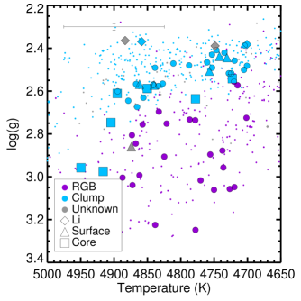
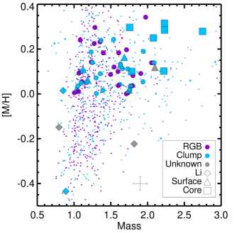
Figure 1: Our sample, with the color indicating the seismic evolutionary state, and the shape of the point indicating the reason the star was selected (circle: mass bins; diamond: identified as lithium-rich by Casey et al. (2019); triangle: measurable surface rotation; square: part of the core rotation sample of Tayar et al. (2019)). For comparison we have shown the APOKASC sample’s overlap with LAMOST data (Gao et al. 2021) as small points in the background.

In this study, we select stars of known mass and evolutionary state for analysis. We use as a basis for selection the APOGEE-Kepler catalog (Pinsonneault et al. 2018). These are stars with asteroseismic parameters from the analysis of Kepler data (Borucki et al. 2010) by five different asteroseismic pipelines, which include theoretical corrections to the scaling relations (White et al. 2011; Sharma et al. 2016; Pinsonneault et al. 2018), as well as empirical corrections to match the mass scale of the clusters in the Kepler field. The estimation of evolutionary states from an ensemble of methods is described in detail in Elsworth et al. (2019).

These stars also have detailed spectroscopic characterization from the APOGEE survey (Majewski et al. 2017), which is a Sloan Digital Sky Survey IV (Blanton et al. 2017) program using the 2.5-meter telescope (Gunn et al. 2006) with the APOGEE spectrograph (Wilson et al. 2019) to collect spectra of stars at moderate resolution (R $\sim$ 22,000) in the H-band. The data are reduced using the ASPCAP pipeline (Nidever et al. 2015; García Pérez et al. 2016) and calibrated to clusters (Mészáros et al. 2013) as well as asteroseismic data (Pinsonneault et al. 2018). For our study, we use the Data Release 14 data (Abolfathi et al. 2018) whose analysis is discussed in detail in Holtzman et al. (2018). We make this choice for consistency with the APOKASC-2 analysis (Pinsonneault et al. 2018) and our target selection, although more recent data releases are now available (Ahumada et al. 2020; Abdurro’uf et al. 2022).

For our analysis, we collected additional, higher resolution spectra for a limited subsample of the APOGEE-Kepler stars. The strength of the lithium line is known to be correlated with temperature, gravity, metallicity, as well as actual lithium abundance, which is correlated with mass, metallicity, evolutionary state. Since we knew our sample would be too small to simultaneously account for all of these variables, we made choices to reduce the number of axes of variation included in our study. Specifically, we restricted ourselves to a limited metallicity range and a limited range in temperature. Our initial sample had very strict cuts on both metallicity and effective temperature (2.1), but to collect a sufficient sample for cross-validation (2.2) and to compare to internal rotation rates (2.4) we were forced to relax these limits slightly. The exact cuts used to select each sample are documented in the appropriate sections.

2.1 Mass Bins

The core of this analysis is the selection of stars in mass bins so we restrict the sample to narrow bins in other stellar parameters. The strengths of the strong Li lines are very sensitive to temperature and are strongest at cooler temperatures for a fixed Li abundance; therefore, we restrict our sample to the region around 4800 K ($\pm$100 K, see Figure 1). In addition, several authors have suggested a metallicity dependence to the lithium distribution (e.g. Martell et al. 2021). To remove this axis of variability, we also choose stars with metallicities between 0.0 and +0.4 dex. We then divide the stars using their asteroseismically measured evolutionary states (Elsworth et al. 2019) into core-helium-burning clump stars and shell-hydrogen-burning first ascent red giants.

Within each sample, we divide the stars between 0.9 and 2.1 solar masses into six mass bins, and identify the brightest stars in each bin. We were able to observe 23 giants and 23 clump stars, which gave us between three and five stars in each bin. As shown in Figure 1, requiring stars at the same temperature but different evolutionary states means that there is a slight offset in surface gravity between our stars in the core-helium-burning phase and those in the shell-hydrogen-burning phase; we do not expect this offset to substantially affect our analysis. We note that at the chosen temperature, the vast majority of the red giant branch stars in our sample should be below the red giant branch bump, which happens around a surface gravity of 2.65 dex for stars at this metallicity, but all should have completed their first dredge up.

2.2 External Cross-validation

Recent work by e.g. Casey et al. (2019) has attempted to identify Li-rich giants and even measure their Li richness from low-resolution (R $\sim$ 10,000) spectra from LAMOST (Large Sky Area Multi-Object Fiber Spectroscopic Telescope; Luo et al. 2015). In order to validate both our abundances and the work being done with lower resolution measurements, we include four stars with asteroseismic measurements that meet our original temperature criteria, but were too faint and/or metal-poor and would not have otherwise been selected. We note that in the course of our analysis, Gao et al. (2021) published Li abundances for several additional stars in our sample and we add those results to our comparison to LAMOST. For illustrative purposes, and to put our smaller sample in context, we also occasionally compare our results to various subsets of the full overlap sample between Gao et al. (2021) and APOKASC-2 (Pinsonneault et al. 2018) throughout this paper. Therefore, we have also shown the Gao et al. (2021) sample as small points in the background of several of our plots for reference, including Figure 1.

2.3 Rapid Rotation

There are well established connections between rapid rotation and Li enhancement (e.g. Carlberg et al. 2012). In addition, in conjunction with mass measurements, rapid rotation has been used as an indicator of potential binary interactions in red giants (Tayar et al. 2015; Ceillier et al. 2017; Daher et al. 2022). To test these connections and their relationship with stellar mass, we added to our sample one giant with a measured spectroscopic rotation velocity and five giants with spot modulation periods (Ceillier et al. 2017) within or just outside our selection criteria. This will allow us to test the mass, evolutionary state, and rotation dependence of the lithium abundance or upper limits at fixed metallicity and sensitivity. We note that several other stars in our sample either had measurements of rotation or had useful upper limits on their rotation velocity inferred from our spectroscopic analysis and we add those to our analysis as well.

2.4 Core Rotation

While previous work has looked for correlations between surface rotation and Li enhancement, in many cases it is the rotation rate of the interior of the star that should provide insight into the connection between rotation and mixing. With asteroseismology, it has become possible to measure the core rotation rates of evolved stars (e.g. Beck et al. 2011; Mosser et al. 2012). We add to our sample a set of seven more massive stars with measured core rotation rates from Tayar et al. (2019) that are close to 4800 K ($\pm$200 K). We also note that after our selection, we discovered that an additional five giants in our sample have measured core rotation rates from Gehan et al. (2018), and so we include that information in our analysis. Our sample selection is documented in Table 1.

3 Observations and Data Reduction

Our higher resolution optical spectra were taken with the High Dispersion Spectrograph (HDS; Noguchi et al. 2002) on the Subaru telescope (Iye et al. 2004) on July 9th and 10th, 2019. The stars ranged in Kepler magnitude from 9 to 12. A non-standard setup using a cross scan rotation angle of $4.533^{\circ}$ and a grating angle of $0.2408^{\circ}$ yielded spectral coverage of $\sim$5700–7050 Å in the red arm. Only data taken from the red side were reduced and used in this analysis. Data were taken with the 2.0”x30” slit and utilized the 0.2”x3 image slicer. The image slicer allows one to potentially reach higher resolving powers of narrower slits with less of a penalty to light lost in typical seeing conditions. However, because the intrinsic broadening of red giants nullifies the benefits of such high spectral resolution, we opted to extract the image slices with a single long aperture in IRAF (Tody 1986, 1993). From measuring the width of ThAr lines, we find that our spectra have a typical resolving power of $R\sim 85,000$ (3.5 km s^-1).

The HDS spectra were reduced with IRAF, following the reduction guidance in the HDS IRAF Reduction Manual . Specialized routines for the overscan correction and non-linearity correction of the data, available from the HDS website, were used in the reduction. Additionally, standard bias subtraction, flat fielding, cosmic ray removal, and scattered light removal were performed. The wavelength solutions were measured from ThAr comparison lamp spectra taken throughout the night, and the solution for each stellar spectrum was interpolated from the comparison lamp spectra taken at the nearest time. The continuum of each echelle order was fit and then divided out by the blaze function. The echelle orders were then intercombined using scombine to create the final one-dimensional spectra. These spectra were cross-correlated with the Hinkle & Wallace (2005) atlas Arcturus spectrum to measure the observed radial velocity, which was used to shift the final spectra to the stellar rest frame.

4 Stellar Characterization

4.1 Lithium Measurements

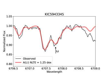
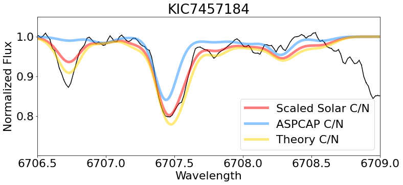
Figure 2: Top: Example best fit spectrum (red) to the observed spectrum (black) of KIC5943345. The Li line is centered in this plot and is the second strongest feature for this star in this wavelength range. Bottom: Our analysis uses scaled-solar (red) CN abundances rather than theoretical (yellow) or directly measured ones (blue) as empirically they seem to provide better fits.

The abundances of Li were measured via synthetic spectrum fitting of the resonance lines in a small bandpass between 6706 and 6709 Å, using the 2019 Version of MOOG (Sneden 1973). In cases of high Li abundance, we also checked the measurement for consistency with the subordinate Li lines at 6104 Å. The line list to generate the spectra draws the atomic information from Ghezzi et al. (2009) and replaces the carbon and nitrogen (CN) data in that work with the new linelists from Sneden et al. (2014). Atmosphere models for each star were interpolated from the grid of MARCS spherical atmosphere models (Plez 2008), using the stellar parameters derived from APOKASC (Pinsonneault et al. 2018), specifically, the corrected temperature, the asteroseismic $\log g$, and the stellar metallicity. A single microturbulence value of 1.5 km s^-1 was used for all stars. To account for the effects of first dredge-up, the carbon and nitrogen abundances were forced to have a ratio of 1.5 while preserving the original scaled-solar sum total number abundance.

A number of atomic features as well as CN molecular features have a large impact on the spectrum in the bandpass of interest, and we tested three different ways of modeling the region. We first generated synthetic spectra by assuming all stars have scaled solar abundances of all elements (other than the C/N adjustment). We then generated a second batch of synthetic spectra where we adopt the APOGEE-measured abundances of C, N, Si, V, Ca, and Fe with the expectation that the atomic and molecular features would be fine-tuned to the star’s individual chemical peculiarities. Finally, we used theoretically predicted C and N abundances from models appropriate to our stars (Tayar et al. 2017). We found cases where using these “fine-tuned” abundances (both APOGEE-measured and theoretical) significantly overestimated or underestimated features nearby the Li lines. Conversely, the scaled solar abundances, while not always the “best” fit to the non-Li features, were more consistently well-fit, and the scaled solar synthetic spectra were ultimately adopted for all of our fits (See Figure 2).

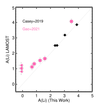
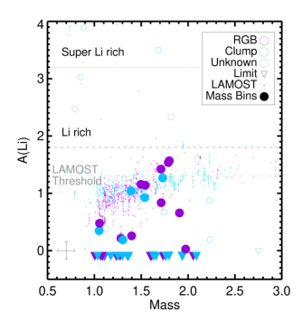
Figure 3: Left: Comparison of the lithium abundances measured in this analysis and the results published using lower-resolution LAMOST spectra from Casey et al. (2019) and Gao et al. (2021). The correlation is quite strong, especially at abundances above A(Li) $\sim$ 1.3 dex, suggesting that LAMOST spectra are sufficient to identify truly lithium-rich giants. We note that our abundances include NLTE corrections whereas the LAMOST values both assume LTE, which could explain some small offsets. Right: Measured lithium abundances and upper limits for the RGB (purple) and clump samples (blue) as well as stars with ambiguous evolutionary states (grey). Stars included as part of the mass sample are shown as large filled symbols, whereas stars included for other reasons are shown as smaller open symbols. The thresholds for lithium richness and super-lithium richness from Deepak & Reddy (2019) are shown for reference. For comparison, published values from LAMOST for stars with metallicities between $0.0-0.4$ dex are shown as tiny open circles; these do not have the same temperature restrictions as our sample. We also have concerns about the LAMOST measurement accuracy for stars below A(Li)$\sim$1.3, marked as ‘LAMOST Threshold’, coming from the left panel.

The adopted broadening is another important factor for the spectral synthesis. The majority of the stars are slow rotators, and the total broadening can be well approximated by a simple Gaussian. To account for slight star-to-star variations in broadening, the neighboring isolated Fe I line at 6750.15 Å was fit with a Gaussian, and the associated full-width at half maximum (FWHM) was adopted for the Li fitting. For the three stars with a previous measurement of $v\sin{i}>6$ km s^-1, we compute separate broadening parameters, using the median FWHM as the instrumental plus macroturbulent velocity component, and the known $v\sin{i}$ (adopting a limb darkening of 0.6) to model the rotation. For 18 stars ($\sim$ 30% of the sample), the adopted FHWM was later reduced to improve the fits.

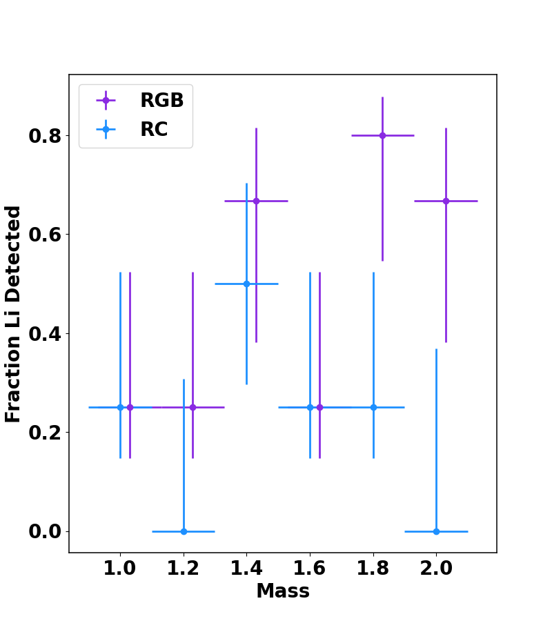
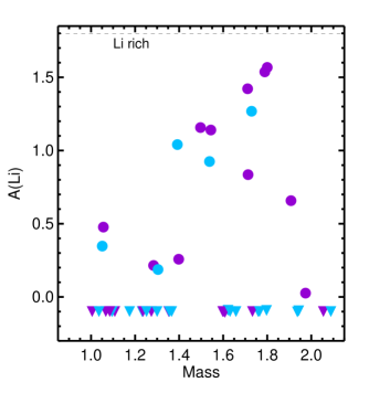
Figure 4: Left: Lithium detection fractions in bins of mass and evolutionary state (RGB in purple and clump in blue), for stars selected along these parameters (Section 2.1). The RGB points are offset by 0.03 $M_{\odot}$ from the bin center for clarity. Error bars are binomial confidence intervals equivalent to 1$\sigma$ probabilities. Right: Similar to the right panel of Figure 3 except that here we show only the measurements and upper limits for the stars chosen as part of the mass and evolutionary state selected sample shown in the left panel.

The fitting procedure was semi-automated. All stars were initially run through an automated procedure where a custom-Python code ran a series of MOOG-generated synthetic spectra with a range of input Li-abundances. The MOOG parameter files for spectral synthesis work with $\Delta$ abundances from the star’s atmosphere file, and the initial set of synthesized $\Delta$$A$(Li) are -3, -2, and -1. The $\chi^{2}$ is computed for the model fits to the data in the narrow wavelength region centered on the Li-lines for the three models, and the $\Delta$$A$(Li) with the minimum $\chi^{2}$ is used as the next best guess in the following iteration. Each iteration uses the best guess plus or minus a step size. When the minimum $\chi^{2}$ is associated with either the minimum or maximum $\Delta$$A$(Li), that $\Delta$$A$(Li) becomes the new best guess, and the step size remains the same. When the middle $\Delta$$A$(Li) of the current iteration has the minimum $\chi^{2}$, a quadratic interpolation of the three pairs defines the next best guess, and the step size decreases in the following progression: 1.0 (the original step size), 0.8, 0.5, 0.2, 0.1, 0.05, and 0.01 dex. This process continues until either a solution is reached (the code reaches the smallest step size) or an upper limit is detected (when the difference between the synthetic models tried in the iteration becomes less than a 1 mÅ). Figure 2 shows an example of one of the stars that was fit the automated procedure.

All of the fits from the automated run were visually inspected, and nine stars were identified at this stage as having poor quality spectra for Li measurements. An additional 16 stars had broadening adjusted to improve the quality of the fits and were rerun through the automated fitting. Four stars (all Li-rich) were fit fully by hand, trading off small variations in the line FWHM parameter and best-fit abundance. At these large line strengths, small errors in the broadening will lead to proportionally larger errors in the abundances. The final results are presented in Table 1. We define our detection limit to be at a feature size of $\sim 5$ mÅ, which corresponds to an upper limit of $A$(Li) $\sim+0.1$ dex. Typical uncertainties in $A$(Li) measurement come from the combination of fitting uncertainties ($\sim$ 0.05–0.1 dex) and propagated errors from stellar parameter uncertainties, which is dominated by the temperature uncertainty. For a temperature uncertainty of 100 K, the associated error in $A$(Li) is 0.13 dex. We adopt a typical uncertainty of 0.15 dex or our sample. Finally, non-local thermodynamic equilibrium (NLTE) corrections were applied. The NLTE corrections were interpolated from the Lind et al. (2009) grid of corrections.

4.2 $v\sin{i}$

We measured $v\sin{i}$ from the spectra using a procedure similar to that used by Carlberg (2014), where the stars had been cross-correlated with radial velocity standard stars broadened with a grid of rotational velocities. Because we did not observe any standard stars with HDS, we modified the procedure to instead measure $v\sin{i}$ using auto-correlation functions. We identified 16 wavelength bins, each 50 Å wide, that are free of strong telluric absorption. We compute the autocorrelation function (ACF) for each star and each bin and record the FWHM of a Gaussian fit to the cross-correlation peak. The star with the smallest average FWHM (KIC 6103934) is selected as a representative slow rotator. Its spectrum is broadened with a range of rotational velocity kernels from 1–6 km s^-1 in 1 km s^-1 steps, and from 6–26 km s^-1 in 2 km s^-1 steps. The ACF fitting procedure is repeated at each rotational velocity, creating a mapping between input rotational velocity and fit FWHM for each wavelength bin. These FWHM-$v\sin{i}$ relationships are interpolated at the measured FWHM for each of the other science targets to estimate the $v\sin{i}$, yielding 16 $v\sin{i}$ measurements per star. In Table 1 we report the measured $v\sin{i}$ (from the mean) and uncertainty (from the standard deviation).

Inherent in this analysis is the assumption that all other broadening contributions (instrumental and macroturbulent) are constant across the sample. Additionally, the macroturbulent velocity of these class-III red giants is typically $\sim 5$ km s^-1 (Gray 2005), larger than the $v\sin{i}$ of many of the slowest rotators. This is why artificially broadening the spectra with input $v\sin{i}$ $\lesssim$ 3-4 km s^-1 has little effect on the measured FWHM. In fact, this method resulted in a measured $v\sin{i}$ of 3.9 km s^-1 for the star selected as the likely smallest broadening. Therefore, we expect our method is unable to recover any $v\sin{i}$ below 4-5 km s^-1. Such limits are consistent with the lack of detected rotational broadening in APOGEE for most of our stars (Tayar et al. 2015; Dixon et al. 2020; Daher et al. 2022; Patton et al. 2023).

5 Analysis

5.1 Validation of Results at Low Resolution

In Figure 3 we compare our measured Li abundances from our analysis of high-resolution Subaru spectra to those estimated from LAMOST low-resolution (Casey et al. 2019) or medium-resolution (Gao et al. 2021) spectra. In general, we find that LAMOST data was entirely sufficient for identifying Li-rich giants. We therefore suggest that with appropriate caution or calibration, they can indeed be used to identify large numbers of Li-rich giants across the galaxy. We do note however that as the Li abundance falls below about A(Li) $\sim$ 1.3 dex, the estimates based on lower-resolution data start to deviate from what we estimate from our higher resolution spectra, suggesting that the detection threshold in LAMOST is slightly underestimated for these cool, high-metallicity giants. This limit is not surprising, since it is approximately where the Li feature becomes weaker than the neighboring Fe-dominated feature near 6707.5 Å, as seen in Figure 2. In the right panel of Figure 3, we plot Li as a function of mass for both our sample and the LAMOST sample. While mass trends are discussed in detail in next section, we note here that the vast majority of LAMOST detections fall below this 1.3 dex threshold and are suspect. Nevertheless, the LAMOST measurements in general show similar trends to our own, with higher lithium abundances for more massive stars (i.e., stars more massive than $\sim$1.8M_☉ tend to be above the LAMOST threshold) and a tentative preponderance of Li-rich red giants at low masses ($\sim$0.8M_☉).

5.2 Correlations with Mass

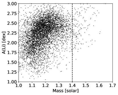
Figure 9: Lithium abundance of stars in the GALAH survey as a function of stellar mass estimated from isochrone fitting. Stars shown have good quality flags, [Fe/H]$=0.2\pm 0.2$ dex and $\log g\in[3.8,4.2]$ dex. The dashed line at mass of 1.4 M_☉is shown for reference, this seems to represent the approximate location of the lithium dip at these metallicities.

Li abundances on the red giant branch are sensitive to a wide range of complicated mixing processes that happen in earlier phases of evolution. One of the core motivations of our analysis was to establish a baseline for normal Li abundances as a function of stellar mass and evolutionary state, so that anomalous Li abundances can be more sensitively identified. In the left panel of Figure 4, we show the fraction of stars with lithium above our detection threshold value as a function of stellar mass and evolutionary state using only the stars selected without reference to their rotation or Li enhanced status. Our detection limit is $\sim-0.1$ dex. We calculated binomial confidence intervals equivalent to 1$\sigma$ for the detection fractions in each mass bin following the prescription given in the Appendix of Burgasser et al. (2003). Even with our relatively small sample, we see expected trends with stellar mass. Lower mass stars (M $<1.3$ M_☉) deplete much of their Li on the main sequence, and we find the detection of Li in the two lowest mass bins is correspondingly low. In the higher mass bins on the RGB, the detection rate is much higher. For the RGB, if we combine the two lowest mass bins and the four highest mass bins we find detection fractions of $25\%^{+19\%}_{-9\%}$ and $60\%^{+10\%}_{-13\%}$, respectively, confirming the overall difference in detectability with stellar mass. However, one high mass bin (centered at 1.6M_☉) shows a much lower fraction of Li detected stars. While this mass is not too far from the lithium dip at these metallicities (Aguilera-Gómez et al. 2018), analysis of the GALAH DR3 data (Buder et al. 2021) indicates that the lithium dip at this metallicity should be at approximately 1.4-1.5M_☉, about half a bin down from where the number of lithium detections drops (see Appendix Figure 9). We therefore suggest that this could indicate a slight offset between the mass scale for the asteroseismic giants and the GALAH dwarfs, a statistical fluctuation, or that there is some sort of as yet unidentified additional lithium destruction happening on the subgiant or lower giant branch at around this mass.

The detection rates of the red clump stars also shows a trend with stellar mass. In the lower mass bins, the Li detection rates are comparable to that seen in the RGB stars. However, the detection rates are much lower at higher masses. Combining the two highest mass bins we find a Li detection rate of only $14\%^{+21\%}_{-5\%}$ for the red clump compared to $75\%^{+5\%}_{-19\%}$ for the first ascent RGB. Such decreases in Li in the more massive stars are not inconsistent with previous results (e.g. from open clusters Carlberg et al. 2016, or the field Martell et al. 2021), but generally there have been limited samples of more massive stars from which to draw conclusions, and so more work is necessary to determine where the depletion happens and the underlying cause. We do not note any mass bins at this metallicity where the detection rates in the clump are significantly above the rates on the red giant branch, something that might be expected if for many stars there was significant Li production and mixing during the ignition of helium burning, as predicted by some theories (Casey et al. 2019; Schwab 2020). According to recent work (Zhang et al. 2021; Deepak & Lambert 2021a), there is no empirical or theoretical indication of obvious Li depletion in the red clump phase and the Li-rich giants can be found at any point of the core-He burning evolution. Lithium in this phase should not be strongly affected by internal mixing. Thus if a giant reaches the clump with a high Li abundance it should preserve it during the clump, and we should observe it to be Li-rich. While our observations are not sufficient to rule out some complex combination of Li production, mixing, and destruction that approximately cancels itself out by the red clump, we do not see evidence for a simple enhancement of Li abundance at the tip of the red giant branch for a large fraction of stars.

In the right panel of Figure 3, we plot the trend of $A$(Li) with mass for all of the stars analyzed in this paper together with the LAMOST measurements. The stars that were chosen based on mass and included in Figure 4 are the filled symbols, whereas the open symbols denote stars selected by us due to their known rotation or for cross-validation. It is only among this latter sample that we find Li-rich stars. We also show the stars selected by mass separately in the right panel of Figure 4. This plot shows that for stars where we have Li detections, the Li abundances tend to be higher for the more massive stars, though the spread of abundances is also large. In general we find that our results are consistent with the larger but less carefully constructed sample from LAMOST. In our sample, we see that there seems to be depletion in the more massive stars (Figure 4, left panel), but no substantial evidence for general Li creation at the tip of the red giant branch.

5.3 Correlations between Lithium and Rotation

Many authors have noted a correlation between rotation rates and lithium enhanced giants (e.g. Fekel & Balachandran 1993; Drake et al. 2002; Carlberg et al. 2016; Delgado Mena et al. 2016; Takeda & Tajitsu 2017) Similarly, on the main sequence and near the lithium dip, there are correlations between lithium and rotation (Anthony-Twarog et al. 2021) Using stars in our sample that have rotation measurements from spots, $v\sin{i}$, or asteroseismology, we search for correlations between rotation and lithium abundance.

5.3.1 Surface Rotation

In general, (see e.g. Massarotti et al. 2008; Tayar et al. 2015; Ceillier et al. 2017; Tayar & Pinsonneault 2018), the rotation rates of giant stars are expected to be slow, with low velocities ($<3$ km s^-1) and long periods (hundreds to thousands of days). However, as part of our sample selection, we included some stars known to rotate rapidly either from their spectroscopic rotation velocities (Tayar et al. 2015) or from their spot rotation periods (Ceillier et al. 2017). In the interim, we have added to this sample any stars that have rotation periods quoted in Gaulme et al. (2020), rotation velocities quoted in Daher et al. (2022), as well as $v\sin{i}$ measurements or limits from the Subaru spectra used in this study. Most of the stars with detectable rotation from any method had measured rotation velocities from the Subaru spectra, and so we have generally plotted those values. However, in a few cases the rotation velocities were near or below our detection limit, but we were able to convert the rotation period to a velocity using the asteroseismic radii to plot those points as rotation detections. For stars that are not spotted, and whose rotation velocities are too slow to measure, we assume an upper limit on the rotation velocity of 4 km s^-1 from the Subaru spectra. In Figure 5, we show all of our estimates of surface rotation, compared to our Li measurements (circles) and limits (downward pointing triangles). We do not see a simple correlation between Li abundance and rotation period in our data, but we do not have very many stars in the super-Li-rich regime where such correlations have been claimed (Du et al. 2021). Consistent with previous authors, we find that lithium-rich giants tend to be rapidly rotating – in our case we detect measureable rotation in all five lithium-rich stars. Four of these were included in this work for their previously known high lithium abundance. However, high rotation did not guarantee lithium-richness. Of the nine stars with detected rotation and no previous lithium measurement, only one was found to be lithium-rich. This is still a higher rate than the much larger population of unmeasurably slow rotators, among which we find zero Li-rich stars. Since find many Li-poor stars among the faster rotators and Li detections among the slower rotators, we suggest that additional data would be required to better study the relationship between lithium and rotation, as the relationship between the two is not simple.

In general, we expect that any of the stars with measurable rotation in our sample are rapidly rotating because they have gained angular momentum on the red giant branch through an interaction with a stellar or substellar companion. While some of the stars in are sample are more massive than the Kraft break (Kraft 1967), and in theory their rotation could be retained from their rapid rotation on the main sequence, in practice, many authors (Massarotti et al. 2008; Tayar et al. 2015; Deheuvels et al. 2015; Carlberg et al. 2016; Ceillier et al. 2017) have found that, in practice, these more massive stars rotate more slowly than expected in the core-helium-burning phase, likely as a result of enhanced angular momentum loss (Tayar & Pinsonneault 2018). We therefore argue that their detected rotation in our analysis is unlikely to be the result of angular momentum retained from the main sequence, and much more likely to be the result of an interaction.

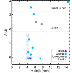
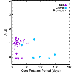
Figure 5: Lithium abundances (circles) and upper limits (downward pointing triangles) compared to rotation measurements (filled symbols) and upper limits (rightward pointing triangles). Xs represent limits in both quantities. Top: We detect rotation in all of the lithium-rich stars, but there is not a strong correlation between the rotation velocity and the lithium abundance. Bottom: No strong correlations are seen between the core rotation period and Li abundance, although stars with strong Li enhancement are less likely to have measured core rotation periods, possibly due to complications in seismology of rapidly rotating stars. Previous data from LAMOST (Gao et al. 2021) are shown as small purple squares.

5.3.2 Core Rotation

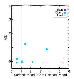
Figure 6: Lithium abundances (circles) and upper limits (downward pointing triangles) compared to the ratio (filled symbols) or limits (rightward triangles or Xs) of the surface rotation period to the core rotation period. As in previous plots, the evolutionary states of the points are indicated by the color (purple for RGB, blue for clump, grey for ambiguous). Stars rotating as a solid body, and therefore presumably with minimal shear forces to drive mixing, would have a ratio of 1 (dotted vertical line). We see no correlation between the core-surface contrast, and therefore the presumed shear forces and rotational mixing, and the detection or abundance of lithium at the stellar surface.

In some theories (e.g. Zahn 1992) it is the internal rotation profile, rather than the surface rate, that should dictate the rotational mixing in the stellar interior and thus the surface abundance of Li. In the past, there was no way of estimating the interior rate, and so it had to be assumed to scale with the surface rotation rate. However, in the past decade it has become possible to infer the rotation rates of the cores of giant stars from their oscillation spectra due to the mixing of the gravity modes in the core with the pressure modes observed at the surface (Beck et al. 2011; Deheuvels et al. 2012; Mosser et al. 2012). In our sample, we specifically targeted a set of stars with core and surface rotation rates available from Tayar et al. (2019). In the course of our analysis, we realized that several stars in our sample also had core rotation measurements available from Gehan et al. (2018). In the lower panel of Figure 5, we show the Li measurements and limits compared to the inferred core rotation period for our stars. We also show on this plot all stars with core rotation measurements available from Gehan et al. (2018) and Li abundances available from LAMOST (Gao et al. 2021) that were in the APOKASC sample; in the interest of sample size for comparison, we do not apply any cuts in effective temperature or metallicity. In the combination of the two data sets, we find no correlation between the core rotation rate and the measurement or abundance of Li at the surface. We do however note that detailed asteroseismology, including the estimation of the interior rotation rate, can be more challenging in active and rapidly rotating stars (Gaulme et al. 2014, but see also Mathur et al. 2020), which might bias core rotation detections against the most Li rich and rapidly rotating stars.

There have also been suggestions (Talon & Charbonnel 2003; Denissenkov et al. 2009) that the local shear forces caused by rotational gradients are important for driving mixing. We therefore show in Figure 6 the ratio of the surface rotation period to the core rotation period, as an estimate of the total internal shears. Stars with a ratio of 1 are consistent with rotating as solid bodies and therefore presumably have minimal shear forces. Most stars have surfaces rotating more slowly than their cores, consistent with the expectations of single star evolution (Tayar & Pinsonneault 2018; Tayar et al. 2019), while there are a few stars whose measurements suggest that their surfaces are rotating faster than their cores (ratios less than 1). While some of these could be measurement errors (Tayar et al. 2019), there are some stars where such rotation profiles seem to be present (Kurtz et al. 2014; Tayar et al. 2022) and they are generally explained with angular momentum transfer from interaction with a companion (e.g. Daher et al. 2022). Should our stars with surfaces rotating faster than their cores prove to be robust, they would be in conflict with theories like that presented in Casey et al. (2019), which suggest that tidal interactions drive Li enhancements that should persist longer than the resulting rotation. More generally, when we look at our stars that have both core and surface rotation estimates or limits and Li abundances, we do not see any strong correlations that would suggest a significant impact of shear mixing on the Li abundances of giants.

5.4 Correlations with Indications of Binarity

Many authors have suggested that Li richness, either on the red giant branch (Carlberg et al. 2016; Aguilera-Gómez et al. 2016; Delgado Mena et al. 2016; Soares-Furtado et al. 2021) or in the red clump (Casey et al. 2019) should be related to the interaction of a giant with a stellar or substellar companion. Because our stars are so exquisitely characterized, we can look at a variety of properties that correlate with binarity and see if they have any correlations with the Li abundance. Because the APOGEE survey used fixed observing times, the stars in the APOKASC sample were often observed multiple times to build up sufficient signal-to-noise; as part of that process APOGEE also makes available measurements of the radial velocity scatter between observations. We show in Figure 7 that while there are a few stars that show evidence of radial velocity variability from a close companion with measured Li, there is no particularly strong correlation between radial velocity scatter and Li abundance, and not all Li-rich stars show evidence for significant radial velocity scatter.

Gaia DR3 (Gaia Collaboration et al. 2022) provides some information about the binary nature of our target stars through the flag NON_SINGLE_STAR, indicating astrometric, spectroscopic, or eclipsing binaries. Only 9 of the 63 giants in the sample are considered non single, all of them with A(Li) $<1.2$ dex. However, the Gaia selection of binaries is not complete, and thus it is not possible with this information alone to discard a possible relation between lithium enhancement and the presence of binary companions (e.g., Sayeed et al. (2023), M. Castro-Tapia et al. 2023, in prep).

One other way of identifying stars that are undergoing or have undergone interactions is through their chemistry. On the red giant branch, we generally expect the mass of a star to correlate with its carbon to nitrogen ratio [C/N] resulting from the mass dependence of the first dredge up, which has been useful for a variety of galactic archaeology purposes (Martig et al. 2016; Ness et al. 2016, J. Roberts, 2023 in prep). We show in Figure 8 that most of the stars in our sample follow this correlation with perhaps slight differences in the relationship for the clump and first ascent giant stars. However, we mark as larger diamonds the Li-rich stars in our sample, and note that all five of them seem to be offset from the general population. We note that this offset for Li-rich giants is not quite as clear in the larger sample from Gao et al. (2021) (shown as smaller background points), and so we encourage further exploration of this point. If it turns out that there is a significant subpopulation of Li-rich red giants with [C/N] ratios that do not match their current masses, it may be a good tracer for stars that have undergone significant mass transfer, and thus their mass during the first dredge up was not the same as their current mass, or indicate that whatever mixing process is impacting the Li abundance is also reaching deeper into the interior, where the [C/N] ratio is set. However, it is also possible that increased rotation leads to poorer spectroscopic fits (Patton et al. 2023) and mis-measured abundances, which can incidentally push stars off of the normal relationship.

Mass transfer or past interaction with a binary companion has also been invoked to explain a different type of unusual objects, young alpha-rich stars (Martig et al. 2015). Although these stars are not thought to be directly related to the phenomenology of Li-rich giants, and our sample giants are intrinsically more metal-rich than most of the galactic alpha-rich population, the young alpha-rich stars also show an unusual behavior in the [C/N]-mass relation (Jofre et al. 2022), with most of them located outside the general population trend, suggesting that offsets in mixing sensitive ratios like the ratio of carbon to nitrogen (E. Bufanda et al., submitted) or the ratio of carbon-12 to carbon-13 (Aguilera-Gómez et al. 2022) may be diagnostic of a wide variety of binary interaction processes.

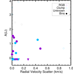
Figure 7: No strong relationships are seen between the radial velocity scatter, a coarse indicator of close binaries, and the lithium abundance, although there is perhaps a slight tendency for stars selected in mass bins to be more likely to have higher radial velocity scatter if they have measured lithium.

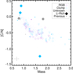
Figure 8: The [C/N] ratio is a mixing diagnostic that correlates with mass for both clump (blue) and RGB (purple) stars. Most sample stars with lithium abundances (circles) and upper limits (downward pointing triangles) follow this correlation. However, stars that are lithium-rich (diamonds) seem to deviate from the relation; deviations tend to be more common in binary evolution products.

6 Discussion

In this work, we have looked at an extremely well-characterized sample of metal-rich red giants in order to get a clearer picture of the distribution of Li in these stars. Previous work has suggested a complex set of processes are impacting Li in red giants, and our analysis seems to agree with that view. Our results are consistent with previous work that super Li rich red giants are rare, that Li-rich giants are more common in the core-helium-burning phase, that rapid surface rotation is often associated with higher Li abundances, but there is no simple relationship. We are also able to demonstrate that:

• LAMOST low and medium resolution spectra are entirely sufficient to accurately identify Li rich giants

• the baseline Li abundance of red giants is likely mass-dependent with more massive red giants generally having higher Li

• in stars more massive than $\sim$ 1.8 M_☉, Li destruction or depletion is likely happening on the upper red giant branch

• core rotation and the core-surface rotational shear seem to be uncorrelated with Li abundance

• Li-rich giants may also have offsets in their carbon to nitrogen ratios

• binarity may be related to the Li rich phenomenon in some cases, but it is likely neither necessary nor sufficient

Given how our targets were selected, we are not able to determine a fraction of enriched RGB or red clump stars. To do this, it is not only necessary to have a large sample of stars, but also, to define first what is considered a truly lithium-rich giant based on the abundances of other stars of similar mass, metallicity, and evolutionary stage. The more massive RGB stars could naturally give rise to more massive enriched red clump stars, while different mechanisms could be acting to produce enrichment in the RGB or less massive red clump giants. Regardless of the specific mechanism, stellar mass is key, and other indicators, such as the carbon-to-nitrogen ratio may provide the additional information needed to distinguish between processes (see e.g., Zhou et al. 2022).

The Li-rich giants continue to be one of the most interesting and frustrating questions in stellar physics. It is clear that these objects have interesting stories to tell about stellar histories that include information about binarity, rotation, mass, metallicity, mixing, and possibly planets, but teasing out the details of those stories has continued to prove challenging. As the number of Li measurements continues to increase, and the complementary knowledge including stellar masses, ages, evolutionary states, binary companions, and so forth becomes more common and precise, we can only hope that eventually some physical explanation, or more likely some combination of physical explanations, will be able to identify the reason for Li enrichment in both a population sense, and on a star-by-star basis.

Table 1: Stellar properties for all stars in our sample.

KICID	2MASS ID	Gaia DR2 ID	Mass	Log(g)	[Fe/H]	[$\alpha$/Fe]	Teff	[C/N]	A(Li)	$\textrm{A(Li)}_{UL}$	Flag	$v\sin(i)$	Period${}_{\textrm{s}}$	Period${}_{\textrm{c}}$	$\sigma_{v}$	State
			M☉	dex	dex	dex	K	dex	dex			km s-1	days	days	km s-1
10461323	2M19114879+4741524	2130879480532813824	2.10000	2.86000	0.118	-0.054	4874.06	-0.616	1.60	0	3	4.065	79.7	-9999.0	-9999.000	U
10522084	2M19024774+4745344	2131483245555109632	1.62200	2.57600	0.043	0.006	4833.55	-0.423	-0.09	1	0	3.264	-9999.0	-9999.0	-9999.000	RC
10550429	2M19492290+4746588	2086419800156327680	1.49700	3.03900	0.087	-0.031	4872.35	-0.685	1.16	0	0	2.885	-9999.0	-9999.0	0.080	RGB
10587122	2M19033449+4748388	2131504857830540032	1.23200	2.48200	0.187	-0.011	4700.81	-0.429	-0.10	1	0	3.529	-9999.0	-9999.0	-9999.000	RC
10722175	2M19122333+4803442	2130984827490239232	1.35300	2.95700	0.232	-0.028	4736.14	-0.472	-0.10	1	0	2.620	-9999.0	22.2	-9999.000	RGB
10793771	2M19213869+4809014	2129414106407732608	2.05500	2.80600	0.139	-0.012	4873.17	-0.596	-0.10	1	0	3.385	-9999.0	-9999.0	-9999.000	RGB
11087371	2M19335280+4836440	2129006870493887744	1.28400	3.06100	0.296	0.013	4750.13	-0.621	0.21	0	0	3.731	-9999.0	inf	-9999.000	RGB
11358669	2M19425925+4911303	2134772129653795328	1.39800	2.89600	0.183	0.008	4755.77	-0.631	0.26	0	0	3.514	-9999.0	16.2	0.002	RGB
11496569	2M19025133+4929261	2132105435996154368	1.59800	2.73300	0.100	-0.007	4786.56	-0.446	-0.10	1	0	3.272	-9999.0	-9999.0	-9999.000	RGB
11550492	2M19065989+4932243	2131326599508772352	1.10800	2.87800	0.055	0.003	4737.56	-0.327	-0.10	1	0	3.218	-9999.0	14.9	-9999.000	RGB
11615224	2M19363394+4938350	2135022302904783360	0.85200	2.38200	0.015	0.024	4700.81	0.119	3.03	0	2	5.653	-9999.0	-9999.0	0.001	RC
1161618	2M19242614+3648478	2050254968627140736	1.18300	2.43800	0.064	0.005	4741.98	-0.265	-0.10	1	3	4.199	158.3	-9999.0	0.021	RC
11618522	2M19421336+4939595	2134930768564971776	1.94300	2.67400	0.189	-0.020	4865.36	-0.695	-0.09	1	0	3.349	-9999.0	-9999.0	0.102	2CL
11649294	2M18562652+4945381	2132278815233502720	1.09600	2.43000	0.100	0.004	4753.13	-0.231	-0.10	1	0	3.337	-9999.0	-9999.0	-9999.000	RC
11969378	2M19390565+5019540	2135158951586941184	1.35600	2.49100	0.090	0.002	4752.94	-0.542	-0.10	1	0	3.059	-9999.0	-9999.0	0.050	RC
12070114	2M19430023+5032393	2135361394864817152	1.63400	2.50700	0.130	0.020	4756.96	-0.243	-0.10	1	4	3.367	-9999.0	-9999.0	0.035	RC
2015820	2M19265758+3728035	2051784840284088064	1.79700	2.56500	0.037	-0.009	4827.03	-0.498	-0.09	1	0	3.816	-9999.0	-9999.0	0.015	RC
2305930	2M19282563+3741232	2051887163583939200	0.88900	2.36900	-0.435	0.165	4858.64	0.329	3.89	0	2	14.427	33.0	-9999.0	0.111	RC
3339894	2M19232223+3826312	2052834599006426240	1.81800	2.38900	-0.223	0.037	4748.55	-0.074	2.33	0	2	7.698	100.0	-9999.0	0.165	U
3459109	2M19404372+3830503	2049134982905799552	1.78900	2.69600	0.036	-0.006	4832.87	-0.671	1.54	0	0	3.424	-9999.0	-9999.0	0.015	RGB
3526061	2M19004471+3836399	2100133252769956224	1.27400	3.01700	0.224	0.002	4770.27	-0.453	-0.10	1	0	2.775	-9999.0	14.3	-9999.000	RGB
3526625	2M19014365+3840029	2100131637861896192	1.12400	2.44400	0.108	0.029	4730.83	-0.182	0.39	0	3	4.187	125.1	-9999.0	0.048	RC
3860253	2M19360616+3854028	2052378026807507968	1.71100	2.84500	0.000	-0.024	4867.49	-0.532	1.42	0	0	3.193	-9999.0	-9999.0	0.033	RGB
3958400	2M19301845+3904562	2053093396558506112	2.08900	2.64500	0.139	-0.009	4878.66	-0.493	-0.10	1	0	3.302	-9999.0	-9999.0	0.018	2CL
4055294	2M19241086+3907357	2052965234733414528	1.60800	2.99300	0.183	0.009	4861.87	-0.686	-0.11	1	0	2.796	-9999.0	-9999.0	0.274	RGB
4474383	2M19370790+3934123	2052437396129089664	1.93700	2.60100	0.054	-0.013	4894.66	-0.728	-0.10	1	0	3.696	-9999.0	-9999.0	0.019	RC
4633907	2M18564805+3946115	2103296925679588992	1.09500	2.38700	0.049	0.027	4704.50	-0.113	-0.10	1	0	4.431	-9999.0	-9999.0	-9999.000	RC
4648485	2M19193317+3945381	2101044507393877248	1.06700	3.05700	0.093	0.049	4726.61	-0.293	-0.10	1	0	2.299	-9999.0	-9999.0	0.044	RGB
4826087	2M19154014+3957514	2101241629211118720	1.60100	2.57300	0.037	0.007	4714.82	-0.517	-0.10	1	0	3.333	16.0	-9999.0	0.007	RGB
4913049	2M19135948+4005110	2101299211835208704	1.00500	3.24800	0.005	0.092	4777.97	-0.251	-0.10	1	0	4.891	-9999.0	-9999.0	0.073	RGB
4931389	2M19353795+4004428	2052513438539100544	1.23600	3.22500	0.142	-0.016	4838.31	-0.460	-0.10	1	0	2.909	-9999.0	-9999.0	0.025	RGB
4937056	2M19411631+4005508	2076298383311466368	1.78500	2.58800	0.101	-0.031	4850.22	-0.393	-0.10	1	5	7.322	82.0	76.2	0.026	RC
5087190	2M19115123+4013021	2100556800967018368	2.08000	2.74700	0.250	-0.021	4904.59	-0.718	-0.04	1	5	4.623	157.0	72.3	0.023	2CL
5095946	2M19230745+4017484	2101132159082055552	1.25200	2.46600	0.140	-0.003	4760.51	-0.391	-0.10	1	0	3.813	-9999.0	-9999.0	0.005	RC
5194072	2M19352306+4023194	2077289970993761408	2.23075	2.63582	0.285	-0.002	4777.94	-0.667	0.19	0	5	4.916	82.7	148.4	0.016	-9999
5383359	2M19482276+4032018	2073730439545220224	1.05100	2.42100	0.035	0.047	4734.59	-0.215	0.35	0	0	3.335	-9999.0	-9999.0	0.068	RC
5534910	2M19285814+4046073	2053573466520267520	2.74800	2.95800	0.279	-0.007	4949.62	-0.860	-0.01	1	5	3.422	102.0	96.4	0.021	2CL
5723909	2M19465321+4058004	2076757223253430144	1.53800	2.51700	0.243	-0.029	4728.04	-0.548	0.92	0	0	3.033	-9999.0	-9999.0	-9999.000	RC
5769244	2M18534059+4102118	2103697147911515136	1.08500	3.04800	0.240	0.019	4719.54	-0.369	-0.10	1	0	2.335	-9999.0	-9999.0	-9999.000	RGB
5791889	2M19283210+4104584	2053597934956366464	1.71300	3.00400	0.197	-0.020	4887.23	-0.664	0.84	0	0	3.131	-9999.0	-9999.0	-9999.000	RGB
5811766	2M19490669+4101352	2076770039436573952	1.80000	2.55600	0.082	-0.003	4720.23	-0.505	1.57	0	0	3.158	-9999.0	-9999.0	-9999.000	RGB
5943345	2M19015661+4114403	2103856267861037824	2.22100	2.61100	0.102	-0.010	4895.35	-0.547	1.25	0	5	4.452	109.0	77.2	-9999.000	RC/2CL
6032639	2M19141495+4118432	2102124743207232128	1.74600	2.56800	0.018	-0.023	4861.82	-0.401	0.68	0	3	5.384	130.0	-9999.0	0.876	RC
6103934	2M18564594+4128038	2103725284237785728	1.54400	2.90600	0.120	-0.034	4824.73	-0.581	1.14	0	0	3.872	-9999.0	-9999.0	-9999.000	RGB
7017044	2M19031889+4230179	2104024012104377344	1.03600	2.40900	0.016	0.022	4746.53	-0.261	-0.10	1	0	3.543	-9999.0	-9999.0	0.006	RC
7097136	2M18562647+4237349	2104920492036763520	1.63100	2.51700	0.133	-0.010	4724.21	-0.496	-0.10	1	0	3.427	-9999.0	-9999.0	-9999.000	RC
7098510	2M18585908+4237588	2104250786376888448	1.30000	2.48000	0.071	-0.006	4787.58	-0.484	-0.10	1	0	3.599	-9999.0	-9999.0	-9999.000	RC
7283405	2M19285388+4250513	2125813583790089088	1.73300	2.75600	0.005	-0.002	4857.25	-0.650	-0.10	1	0	3.070	-9999.0	35.0	0.094	RGB
7351098	2M19114520+4255162	2102592482324682368	2.23000	2.97500	0.315	-0.003	4916.38	-0.756	0.87	0	5	3.292	125.0	34.2	0.045	2CL
7457184	2M19410681+4303056	2078012762449199360	1.97400	2.73600	0.342	0.007	4778.26	-0.782	0.03	0	0	2.627	-9999.0	-9999.0	-9999.000	RGB
7499531	2M18414542+4308496	2116826072661485312	1.90800	2.75200	0.091	0.080	4821.27	-0.339	0.66	0	0	3.223	-9999.0	-9999.0	0.481	RGB
7585122	2M18500383+4316049	2105182004005398656	1.36600	2.50100	0.239	-0.004	4705.34	-0.570	-0.10	1	0	3.159	-9999.0	-9999.0	0.114	RC
8197210	2M20033477+4402323	2075875170103511040	1.76500	2.56700	0.035	-0.027	4867.05	-0.463	-0.10	1	0	3.309	-9999.0	-9999.0	0.002	RC
8540767	2M18502221+4436052	2105409499833058048	0.79500	2.36400	-0.149	0.026	4883.28	-0.055	2.47	0	2	6.218	-9999.0	-9999.0	0.052	U
8555914	2M19210796+4437273	2126987037571830912	1.17500	2.45800	0.050	-0.020	4719.37	-0.242	-0.10	1	0	3.164	-9999.0	-9999.0	0.018	RC
8782196	2M20023887+4455347	2082151839616048768	1.05600	2.72500	0.011	0.034	4701.62	-0.215	0.48	0	0	2.733	-9999.0	-9999.0	0.017	RGB
8872709	2M19053513+4506383	2106419538702242304	1.39200	2.49100	0.016	0.015	4838.61	-0.470	1.04	0	0	3.138	-9999.0	-9999.0	0.057	RC
8879518	2M19181645+4506527	2127061804363014272	1.68400	2.57200	0.163	-0.004	4839.97	-1.222	3.50	0	3	4.924	109.0	-9999.0	0.003	RC
9335570	2M19151622+4553087	2127334551963243136	1.30400	2.47100	0.001	-0.001	4811.13	-0.532	0.19	0	0	3.343	-9999.0	-9999.0	-9999.000	RC
9469212	2M19341942+4604596	2128063768695712256	1.75600	2.54200	0.297	-0.013	4722.75	-0.613	-0.10	1	5	3.907	68.4	128.6	-9999.000	RC
9491316	2M20013827+4604468	2085315233343597696	1.72900	2.63100	0.111	-0.020	4856.02	-0.505	1.27	0	0	3.009	-9999.0	-9999.0	0.436	RC/2CL
9575645	2M19022297+4615098	2106548314702107264	1.65800	2.57100	0.113	0.006	4841.36	-0.426	-0.10	1	0	3.201	-9999.0	-9999.0	0.026	RC

Note. — Lithium values quoted here include NLTE corrections. Mass refers to the empirically corrected version of the seismic scaling relation mass, equivalent to the APOKASC2 seismic mass from Pinsonneault et al. (2018). Similarly, $\log g$ refers to the APOKASC2 seismic $\log g$. [Fe/H], [$\alpha$/Fe], T_eff, and [C/N] values are taken from APOGEE DR14. $\sigma_{v}$ refers to the radial velocity scatter from APOGEE DR14. Lithium upper limits are marked as 1 in the A(Li)_UL column. Period_s refers to the best estimate for the surface rotation period from Ceillier et al. (2017) or Gaulme et al. (2020). Period_c refers to the core rotation period from Tayar et al. (2019) or Gehan et al. (2018). Stars without measured surface or core rotation periods are allocated a period of -9999. Flag indicates the reason for selection, 0: Mass bins, 2: lithium rich, 3: spots, 4: velocity, 5: Tayar et al. (2019). Evolutionary states are taken from Pinsonneault et al. (2018) and described further in Elsworth et al. (2019), U: Uncertain, RGB: red giant branch, RC: red clump, 2CL: secondary clump, -9999: no answer was returned

Appendix A Lithium Dip

References

- Abdurro’uf et al. (2022) Abdurro’uf, Accetta, K., Aerts, C., et al. 2022, ApJS, 259, 35, doi: 10.3847/1538-4365/ac4414
- Abolfathi et al. (2018) Abolfathi, B., Aguado, D. S., Aguilar, G., et al. 2018, ApJS, 235, 42, doi: 10.3847/1538-4365/aa9e8a
- Aguilera-Gómez et al. (2016) Aguilera-Gómez, C., Chanamé, J., Pinsonneault, M. H., & Carlberg, J. K. 2016, ApJ, 829, 127, doi: 10.3847/0004-637X/829/2/127
- Aguilera-Gómez et al. (2022) Aguilera-Gómez, C., Jones, M. I., & Chanamé, J. 2022, arXiv e-prints, arXiv:2207.08905. https://arxiv.org/abs/2207.08905
- Aguilera-Gómez et al. (2018) Aguilera-Gómez, C., Ramírez, I., & Chanamé, J. 2018, A&A, 614, A55, doi: 10.1051/0004-6361/201732209
- Ahumada et al. (2020) Ahumada, R., Allende Prieto, C., Almeida, A., et al. 2020, ApJS, 249, 3, doi: 10.3847/1538-4365/ab929e
- Alexander (1967) Alexander, J. B. 1967, The Observatory, 87, 238
- Anthony-Twarog et al. (2021) Anthony-Twarog, B. J., Deliyannis, C. P., & Twarog, B. A. 2021, AJ, 161, 159, doi: 10.3847/1538-3881/abe0b7
- Badenes et al. (2018) Badenes, C., Mazzola, C., Thompson, T. A., et al. 2018, ApJ, 854, 147, doi: 10.3847/1538-4357/aaa765
- Beck et al. (2011) Beck, P. G., Bedding, T. R., Mosser, B., et al. 2011, Science, 332, 205, doi: 10.1126/science.1201939
- Bedding et al. (2011) Bedding, T. R., Mosser, B., Huber, D., et al. 2011, Nature, 471, 608, doi: 10.1038/nature09935
- Blanton et al. (2017) Blanton, M. R., Bershady, M. A., Abolfathi, B., et al. 2017, AJ, 154, 28, doi: 10.3847/1538-3881/aa7567
- Borucki et al. (2010) Borucki, W. J., Koch, D., Basri, G., et al. 2010, Science, 327, 977, doi: 10.1126/science.1185402
- Brown et al. (1989) Brown, J. A., Sneden, C., Lambert, D. L., & Dutchover, Jr., E. 1989, ApJS, 71, 293, doi: 10.1086/191375
- Buder et al. (2021) Buder, S., Sharma, S., Kos, J., et al. 2021, MNRAS, 506, 150, doi: 10.1093/mnras/stab1242
- Burgasser et al. (2003) Burgasser, A. J., Kirkpatrick, J. D., Reid, I. N., et al. 2003, ApJ, 586, 512, doi: 10.1086/346263
- Cameron & Fowler (1971) Cameron, A. G. W., & Fowler, W. A. 1971, ApJ, 164, 111, doi: 10.1086/150821
- Carlberg (2014) Carlberg, J. K. 2014, AJ, 147, 138, doi: 10.1088/0004-6256/147/6/138
- Carlberg et al. (2016) Carlberg, J. K., Cunha, K., & Smith, V. V. 2016, ApJ, 827, 129, doi: 10.3847/0004-637X/827/2/129
- Carlberg et al. (2012) Carlberg, J. K., Cunha, K., Smith, V. V., & Majewski, S. R. 2012, ApJ, 757, 109, doi: 10.1088/0004-637X/757/2/109
- Casey et al. (2019) Casey, A. R., Ho, A. Y. Q., Ness, M., et al. 2019, ApJ, 880, 125, doi: 10.3847/1538-4357/ab27bf
- Ceillier et al. (2017) Ceillier, T., Tayar, J., Mathur, S., et al. 2017, A&A, 605, A111, doi: 10.1051/0004-6361/201629884
- Cui et al. (2012) Cui, X.-Q., Zhao, Y.-H., Chu, Y.-Q., et al. 2012, Research in Astronomy and Astrophysics, 12, 1197, doi: 10.1088/1674-4527/12/9/003
- Daher et al. (2022) Daher, C. M., Badenes, C., Tayar, J., et al. 2022, MNRAS, 512, 2051, doi: 10.1093/mnras/stac590
- De Silva et al. (2015) De Silva, G. M., Freeman, K. C., Bland-Hawthorn, J., et al. 2015, MNRAS, 449, 2604, doi: 10.1093/mnras/stv327
- Deepak & Lambert (2021a) Deepak, & Lambert, D. L. 2021a, MNRAS, 507, 205, doi: 10.1093/mnras/stab2022
- Deepak & Lambert (2021b) —. 2021b, MNRAS, 505, 642, doi: 10.1093/mnras/stab1195
- Deepak et al. (2020) Deepak, Lambert, D. L., & Reddy, B. E. 2020, MNRAS, doi: 10.1093/mnras/staa729
- Deepak & Reddy (2019) Deepak, & Reddy, B. E. 2019, MNRAS, 484, 2000, doi: 10.1093/mnras/stz128
- Deheuvels et al. (2015) Deheuvels, S., Ballot, J., Beck, P. G., et al. 2015, A&A, 580, A96, doi: 10.1051/0004-6361/201526449
- Deheuvels et al. (2012) Deheuvels, S., García, R. A., Chaplin, W. J., et al. 2012, ApJ, 756, 19, doi: 10.1088/0004-637X/756/1/19
- Delgado Mena et al. (2016) Delgado Mena, E., Tsantaki, M., Sousa, S. G., et al. 2016, A&A, 587, A66, doi: 10.1051/0004-6361/201527196
- Denissenkov & Herwig (2004) Denissenkov, P. A., & Herwig, F. 2004, ApJ, 612, 1081, doi: 10.1086/422575
- Denissenkov et al. (2009) Denissenkov, P. A., Pinsonneault, M., & MacGregor, K. B. 2009, ApJ, 696, 1823, doi: 10.1088/0004-637X/696/2/1823
- Dixon et al. (2020) Dixon, D., Tayar, J., & Stassun, K. G. 2020, AJ, 160, 12, doi: 10.3847/1538-3881/ab9080
- Drake et al. (2002) Drake, N. A., de la Reza, R., da Silva, L., & Lambert, D. L. 2002, AJ, 123, 2703, doi: 10.1086/339968
- Du et al. (2021) Du, M.-h., Bi, S.-l., Shi, J.-r., & Yan, H.-l. 2021, Chinese Astron. Astrophys., 45, 45, doi: 10.1016/j.chinastron.2021.02.003
- Elsworth et al. (2019) Elsworth, Y., Hekker, S., Johnson, J. A., et al. 2019, MNRAS, 489, 4641, doi: 10.1093/mnras/stz2356
- Fekel & Balachandran (1993) Fekel, F. C., & Balachandran, S. 1993, ApJ, 403, 708, doi: 10.1086/172242
- Gaia Collaboration et al. (2022) Gaia Collaboration, Arenou, F., Babusiaux, C., et al. 2022, arXiv e-prints, arXiv:2206.05595. https://arxiv.org/abs/2206.05595
- Gao et al. (2019) Gao, Q., Shi, J.-R., Yan, H.-L., et al. 2019, ApJS, 245, 33, doi: 10.3847/1538-4365/ab505c
- Gao et al. (2021) —. 2021, ApJ, 914, 116, doi: 10.3847/1538-4357/abf841
- García Pérez et al. (2016) García Pérez, A. E., Allende Prieto, C., Holtzman, J. A., et al. 2016, AJ, 151, 144, doi: 10.3847/0004-6256/151/6/144
- Gaulme et al. (2014) Gaulme, P., Jackiewicz, J., Appourchaux, T., & Mosser, B. 2014, ApJ, 785, 5, doi: 10.1088/0004-637X/785/1/5
- Gaulme et al. (2020) Gaulme, P., Jackiewicz, J., Spada, F., et al. 2020, A&A, 639, A63, doi: 10.1051/0004-6361/202037781
- Gehan et al. (2018) Gehan, C., Mosser, B., Michel, E., Samadi, R., & Kallinger, T. 2018, A&A, 616, A24, doi: 10.1051/0004-6361/201832822
- Ghezzi et al. (2009) Ghezzi, L., Cunha, K., Smith, V. V., et al. 2009, ApJ, 698, 451, doi: 10.1088/0004-637X/698/1/451
- Gilmore et al. (2012) Gilmore, G., Randich, S., Asplund, M., et al. 2012, The Messenger, 147, 25
- Gratton et al. (2000) Gratton, R. G., Sneden, C., Carretta, E., & Bragaglia, A. 2000, A&A, 354, 169
- Gray (2005) Gray, D. F. 2005, The Observation and Analysis of Stellar Photospheres
- Gunn et al. (2006) Gunn, J. E., Siegmund, W. A., Mannery, E. J., et al. 2006, AJ, 131, 2332, doi: 10.1086/500975
- Hinkle & Wallace (2005) Hinkle, K., & Wallace, L. 2005, in Astronomical Society of the Pacific Conference Series, Vol. 336, Cosmic Abundances as Records of Stellar Evolution and Nucleosynthesis, ed. I. Barnes, Thomas G. & F. N. Bash, 321
- Holtzman et al. (2018) Holtzman, J. A., Hasselquist, S., Shetrone, M., et al. 2018, AJ, 156, 125, doi: 10.3847/1538-3881/aad4f9
- Iye et al. (2004) Iye, M., Karoji, H., Ando, H., et al. 2004, PASJ, 56, 381, doi: 10.1093/pasj/56.2.381
- Jofre et al. (2022) Jofre, P., Jorissen, A., Aguilera-Gomez, C., et al. 2022, arXiv e-prints, arXiv:2207.11084. https://arxiv.org/abs/2207.11084
- Kirby et al. (2012) Kirby, E. N., Fu, X., Guhathakurta, P., & Deng, L. 2012, ApJ, 752, L16, doi: 10.1088/2041-8205/752/1/L16
- Kjeldsen & Bedding (1995) Kjeldsen, H., & Bedding, T. R. 1995, A&A, 293, 87
- Knauth et al. (2003) Knauth, D. C., Federman, S. R., & Lambert, D. L. 2003, ApJ, 586, 268, doi: 10.1086/346264
- Kraft (1967) Kraft, R. P. 1967, ApJ, 150, 551, doi: 10.1086/149359
- Kumar et al. (2020) Kumar, Y. B., Reddy, B. E., Campbell, S. W., et al. 2020, Nature Astronomy, 4, 1059, doi: 10.1038/s41550-020-1139-7
- Kurtz et al. (2014) Kurtz, D. W., Saio, H., Takata, M., et al. 2014, ArXiv e-prints. https://arxiv.org/abs/1405.0155
- Lagarde et al. (2019) Lagarde, N., Reylé, C., Robin, A. C., et al. 2019, A&A, 621, A24, doi: 10.1051/0004-6361/201732433
- Lind et al. (2009) Lind, K., Asplund, M., & Barklem, P. S. 2009, A&A, 503, 541, doi: 10.1051/0004-6361/200912221
- Luo et al. (2015) Luo, A. L., Zhao, Y.-H., Zhao, G., et al. 2015, Research in Astronomy and Astrophysics, 15, 1095, doi: 10.1088/1674-4527/15/8/002
- Magrini et al. (2021) Magrini, L., Lagarde, N., Charbonnel, C., et al. 2021, A&A, 651, A84, doi: 10.1051/0004-6361/202140935
- Majewski et al. (2017) Majewski, S. R., Schiavon, R. P., Frinchaboy, P. M., et al. 2017, AJ, 154, 94, doi: 10.3847/1538-3881/aa784d
- Martell et al. (2021) Martell, S. L., Simpson, J. D., Balasubramaniam, A. G., et al. 2021, MNRAS, 505, 5340, doi: 10.1093/mnras/stab1356
- Martig et al. (2015) Martig, M., Rix, H.-W., Silva Aguirre, V., et al. 2015, MNRAS, 451, 2230, doi: 10.1093/mnras/stv1071
- Martig et al. (2016) Martig, M., Fouesneau, M., Rix, H.-W., et al. 2016, MNRAS, 456, 3655, doi: 10.1093/mnras/stv2830
- Massarotti et al. (2008) Massarotti, A., Latham, D. W., Stefanik, R. P., & Fogel, J. 2008, AJ, 135, 209, doi: 10.1088/0004-6256/135/1/209
- Mathur et al. (2020) Mathur, S., Santos, A. R. G., García, R. A., et al. 2020, in Astrophysics and Space Science Proceedings, Vol. 57, Dynamics of the Sun and Stars; Honoring the Life and Work of Michael J. Thompson, ed. M. J. P. F. G. Monteiro, R. A. García, J. Christensen-Dalsgaard, & S. W. McIntosh, 115–120, doi: 10.1007/978-3-030-55336-4_12
- Mészáros et al. (2013) Mészáros, S., Holtzman, J., García Pérez, A. E., et al. 2013, AJ, 146, 133, doi: 10.1088/0004-6256/146/5/133
- Ming-hao et al. (2021) Ming-hao, D., Shao-lan, B., Jian-rong, S., & Hong-liang, Y. 2021, Chinese Astron. Astrophys., 45, 45, doi: 10.1016/j.chinastron.2021.02.003
- Moe et al. (2019) Moe, M., Kratter, K. M., & Badenes, C. 2019, ApJ, 875, 61, doi: 10.3847/1538-4357/ab0d88
- Mori et al. (2021) Mori, K., Kusakabe, M., Balantekin, A. B., Kajino, T., & Famiano, M. A. 2021, MNRAS, 503, 2746, doi: 10.1093/mnras/stab595
- Mosser et al. (2012) Mosser, B., Goupil, M. J., Belkacem, K., et al. 2012, A&A, 548, A10, doi: 10.1051/0004-6361/201220106
- Mosser et al. (2014) Mosser, B., Benomar, O., Belkacem, K., et al. 2014, A&A, 572, L5, doi: 10.1051/0004-6361/201425039
- Ness et al. (2016) Ness, M., Hogg, D. W., Rix, H.-W., et al. 2016, ApJ, 823, 114, doi: 10.3847/0004-637X/823/2/114
- Nidever et al. (2015) Nidever, D. L., Holtzman, J. A., Allende Prieto, C., et al. 2015, AJ, 150, 173, doi: 10.1088/0004-6256/150/6/173
- Noguchi et al. (2002) Noguchi, K., Aoki, W., Kawanomoto, S., et al. 2002, PASJ, 54, 855, doi: 10.1093/pasj/54.6.855
- Patton et al. (2023) Patton, R. A., Pinsonneault, M. H., Cao, L., et al. 2023, arXiv e-prints, arXiv:2303.08151, doi: 10.48550/arXiv.2303.08151
- Pinsonneault et al. (2018) Pinsonneault, M. H., Elsworth, Y. P., Tayar, J., et al. 2018, ArXiv e-prints. https://arxiv.org/abs/1804.09983
- Plez (2008) Plez, B. 2008, Physica Scripta Volume T, 133, 014003, doi: 10.1088/0031-8949/2008/T133/014003
- Sackmann & Boothroyd (1992) Sackmann, I. J., & Boothroyd, A. I. 1992, ApJ, 392, L71, doi: 10.1086/186428
- Sayeed et al. (2023) Sayeed, M., Ness, M. K., Montet, B. T., et al. 2023, arXiv e-prints, arXiv:2306.03323. https://arxiv.org/abs/2306.03323
- Schwab (2020) Schwab, J. 2020, ApJ, 901, L18, doi: 10.3847/2041-8213/abb45f
- Sestito & Randich (2005) Sestito, P., & Randich, S. 2005, A&A, 442, 615, doi: 10.1051/0004-6361:20053482
- Sharma et al. (2016) Sharma, S., Stello, D., Bland-Hawthorn, J., Huber, D., & Bedding, T. R. 2016, ApJ, 822, 15, doi: 10.3847/0004-637X/822/1/15
- Shetrone et al. (2019) Shetrone, M., Tayar, J., Johnson, J. A., et al. 2019, ApJ, 872, 137, doi: 10.3847/1538-4357/aaff66
- Siess & Livio (1999) Siess, L., & Livio, M. 1999, MNRAS, 308, 1133, doi: 10.1046/j.1365-8711.1999.02784.x
- Singh et al. (2019) Singh, R., Reddy, B. E., Bharat Kumar, Y., & Antia, H. M. 2019, ApJ, 878, L21, doi: 10.3847/2041-8213/ab2599
- Sneden et al. (2014) Sneden, C., Lucatello, S., Ram, R. S., Brooke, J. S. A., & Bernath, P. 2014, ApJS, 214, 26, doi: 10.1088/0067-0049/214/2/26
- Sneden (1973) Sneden, C. A. 1973, PhD thesis, The Univerisity of Texas at Austin.
- Soares-Furtado et al. (2021) Soares-Furtado, M., Cantiello, M., MacLeod, M., & Ness, M. K. 2021, AJ, 162, 273, doi: 10.3847/1538-3881/ac273c
- Sun et al. (2022) Sun, Q., Deliyannis, C. P., Twarog, B. A., et al. 2022, MNRAS, 513, 5387, doi: 10.1093/mnras/stac1251
- Takeda & Tajitsu (2017) Takeda, Y., & Tajitsu, A. 2017, PASJ, 69, 74, doi: 10.1093/pasj/psx057
- Talon & Charbonnel (2003) Talon, S., & Charbonnel, C. 2003, A&A, 405, 1025, doi: 10.1051/0004-6361:20030672
- Tayar et al. (2019) Tayar, J., Beck, P. G., Pinsonneault, M. H., García, R. A., & Mathur, S. 2019, ApJ, 887, 203, doi: 10.3847/1538-4357/ab558a
- Tayar & Pinsonneault (2018) Tayar, J., & Pinsonneault, M. H. 2018, ApJ, 868, 150, doi: 10.3847/1538-4357/aae979
- Tayar et al. (2015) Tayar, J., Ceillier, T., García-Hernández, D. A., et al. 2015, ApJ, 807, 82, doi: 10.1088/0004-637X/807/1/82
- Tayar et al. (2017) Tayar, J., Somers, G., Pinsonneault, M. H., et al. 2017, ApJ, 840, 17, doi: 10.3847/1538-4357/aa6a1e
- Tayar et al. (2022) Tayar, J., Moyano, F. D., Soares-Furtado, M., et al. 2022, ApJ, 940, 23, doi: 10.3847/1538-4357/ac9312
- Tody (1986) Tody, D. 1986, in Society of Photo-Optical Instrumentation Engineers (SPIE) Conference Series, Vol. 627, Instrumentation in astronomy VI, ed. D. L. Crawford, 733, doi: 10.1117/12.968154
- Tody (1993) Tody, D. 1993, in Astronomical Society of the Pacific Conference Series, Vol. 52, Astronomical Data Analysis Software and Systems II, ed. R. J. Hanisch, R. J. V. Brissenden, & J. Barnes, 173
- White et al. (2011) White, T. R., Bedding, T. R., Stello, D., et al. 2011, ApJ, 742, L3, doi: 10.1088/2041-8205/742/1/L3
- Wilson et al. (2019) Wilson, J. C., Hearty, F. R., Skrutskie, M. F., et al. 2019, arXiv e-prints. https://arxiv.org/abs/1902.00928
- Yan et al. (2021) Yan, H.-L., Zhou, Y.-T., Zhang, X., et al. 2021, Nature Astronomy, 5, 86, doi: 10.1038/s41550-020-01217-8
- Zahn (1992) Zahn, J.-P. 1992, A&A, 265, 115
- Zhang et al. (2021) Zhang, J., Shi, J.-R., Yan, H.-L., et al. 2021, ApJ, 919, L3, doi: 10.3847/2041-8213/ac224c
- Zhang et al. (2020) Zhang, X., Jeffery, C. S., Li, Y., & Bi, S. 2020, ApJ, 889, 33, doi: 10.3847/1538-4357/ab5e89
- Zhou et al. (2022) Zhou, Y., Wang, C., Yan, H., et al. 2022, ApJ, 931, 136, doi: 10.3847/1538-4357/ac6b3a