Retransmission performance in a
stochastic geometric cellular network model

Abstract

Suppose sender-receiver transmission links in a downlink network at given data rate are subject to fading, path-loss and inter-cell interference, and that transmissions either pass, suffer loss, or incur retransmission delay. We introduce a method to obtain the average activity level of the system required for handling the buffered work and from this derive the resulting coverage probability and key performance measures. The technique involves a family of stationary buffer distributions which is used to solving iteratively a nonlinear balance equation for the unknown busy-link probability and then identifying throughput, loss probability and delay. The results allow for straightforward numerical investigation of performance indicators, are in special cases explicit, and may be easily used to study the trade-off between reliability, latency, and data rate.

I Introduction

The recent letter [B2022] highlights the importance of analyzing spatial and temporal stationarity in queues, and points to the need for a tractable computational setting for certain classes of queueing networks including cellular networks for wireless communication. We consider a simplified slotted time Poisson-Voronoi type stochastic model of a wireless communication system and analyze conditions under which such systems may operate long term, hence addressing some of the challenges indicated in [B2022]. Our particular focus is towards highly reliable controlled delay systems where emitter nodes store failed transmissions in buffers and retransmit. In this sense we aim at identifying a generic stochastic model set-up to assist investigation of long-run ultrareliable and low-latency communication for 5G wireless networks, [BDP2018].

Stochastic geometry provides widely used tools and techniques for modeling and performance analysis of wireless communication systems. Random point processes are used to represent spatially deployed transmission nodes while additional random markings model spatial and temporal features of signal transmission links. Nodes which transmit simultaneously on a common channel cause interference between the actively involved links. Hence, within the network, competition emerges for shared capacity resources, leading to a number of issues related to this type of modeling, about system stability, stationarity in time and space, loss versus delay, etc. The use of planar Poisson point processes and stochastic geometry to study radio terminals can be traced back at least to [TK1984], followed by e.g. [S1992] and [IHV1998]. Comprehensive and rigorous presentations of stochastic geometry and its applications for wireless networks are covered in [BB2009] and [H2012]. Some of the more recent contributions relying on stochastic geometric methods have analyzed downlink cellular networks [ABG2011], uplink cellular networks [NDA2013], interference alignment [GWF2016], D2D networks [SB2017, YLQ2016], and performance of full duplex systems [LPH2018]. A few studies treat elements of retransmission or buffer mechanisms using a stochastic geometric approach; in [YQ2018] each base station is equipped with an infinite size buffer and [NMH2014] considers cooperating base stations and a setting where data is successfully transmitted if at most one retransmission is required.

I-A Poisson-Voronoi stochastic geometric models

We consider a wireless network with two types of nodes which represent user equipment (UE) and base stations (BS) and adhere to the simplified but common approach that the placement of nodes is initially random in the spatial domain but static in time. A transmission link consists of an emitter-receiver pair and connects a BS node with a UE node. It is convenient to simply place the nodes in all of $\mathbb{R}^{d}$, $d\geq 1$, to avoid boundary effects, and make the assumption of independence between disjoint spatial regions in the sense of the Poisson point process on $\mathbb{R}^{d}$. The transmission of signals between pairs of the nodes is further assumed to be synchronized and slotted in time. In a fixed slot each sender attempts to transmit the equivalent of one symbol. The emergence of emitter-receiver pairs and hence the pattern of signal transmit connections will rely on the principle of shortest distance measured from a UE to the nearest BS. As a consequence, the service domains of the BS-nodes form exactly as the random spatial cells known as the Poisson-Voronoi tesselation. In this framework, a number of detailed assumptions are required in order to characterize how transmission links emerge, whether transmitted signals are successfully received or not, and how the performance of the system might be inferred. Various examples and research directions are discussed in the general literature sources listed above.

Our present approach combines some of the typical and well-established model assumptions and techniques with newly developed tools. Thus, following a tradition in wireless network modeling, signals are subject to Rayleigh fast fading and path loss along a radially decreasing attenuation function (either bounded or singular at zero-distance). Moreover, simultaneous random fading variables are assumed spatially independent and interference caused by shared communication links is treated as added noise. For now we restrict to downlink traffic for which the BS is the transmitter and the UE the receiver. Among novel tools we introduce a counting method based on the traditional iterative Lindley equation method for recording retransmission requests as well as losses at the sender nodes. This allows us to present a consistent network model where failed transmission attempts are either stored in a buffer and retransmitted after some queueing delay, or lost due to lack of available buffer space. The main contribution is a technique to determine for given link data rate input whether the system is able to process the work over time and, if so, quantify the resulting loss and delay.

Briefly, we assume that new traffic arrives randomly to the system, such that in any given time slot each designated transmission link is requested to handle a new signal with probability $p$, $0\leq p\leq 1$, independently between slots and between emitters. In response, the system needs to find a mode of operation in which a typical emitter is active with some probability $q$, $p\leq q\leq 1$, the busy-link probability, which is large enough to allow new signal transmissions as well as retransmissions in case of failed attempts. Interference in our setup occurs between cells, not within cells, and we consider the successful coverage of signals to be determined by a meanfield criteria of the type $\mathrm{SINR}>T$, where $\mathrm{SINR}$ is a suitable signal to interference-and-noise ratio and $T>0$ a fixed threshold value. The results are parameterized by an integer $K$ which represents the maximal buffer size. For finite $K$ and given $p$, we use the coverage probability $V_{T}(q)=\mathbb{P}(\mathrm{SINR}>T)$ to identify the stationary buffer distribution, which in particular involves solving a specific balance equation to obtain $q$ as function of $p$. From this we obtain the buffer size distribution and efficient means to quantify loss and delay. The simplest case $K=0$ is a pure-loss model with no retransmission and hence $q=p$. The main results in this work apply to the finite buffer model with $K\geq 1$. which allows studying the trade-off between smaller loss and longer delay as the buffer size increases. For the idealized case of an infinite buffer and hence no-loss, we identify a region of stability. There exists a critical $p_{c}$, such that for traffic rates $p<p_{c}$, there is a busy link probability $q$, $p<q<1$, for which the wireless network model can operate in a steady-state sustained by a geometric buffer size distribution.

II Network model

II-A Voronoi cells acting as servers

We let $\Phi_{\mathrm{UE}}=\{x_{i}\}$ and $\Phi_{\mathrm{BS}}=\{x_{j}\}$ denote two independent Poisson point processes in $\mathbb{R}^{d}$ with intensity measures $\lambda_{0}\,dx$ and $\lambda_{1}\,dx$, respectively, representing the locations of nonmobile user equipment and locations of base stations. Formally, we consider a generic probability space $(\Omega,\mathcal{F},\mathbb{P})$ and define the point processes $\Phi$ ($\Phi_{\mathrm{BS}}$ or $\Phi_{\mathrm{UE}}$) as random counting measures on $(\mathbb{R}^{d},\mathcal{B})$, where $\mathcal{B}$ denotes the Borel sets on $\mathbb{R}^{d}$. Hence, $\Phi:\Omega\times\mathcal{B}\mapsto\{0,1,\dots,+\infty\}$ is a mapping such that $\omega\mapsto\Phi(\omega,B)$ is an (extended) integer-valued random variable for each $B\in\mathcal{B}$ and $B\mapsto\Phi(\omega,B)$ is a Borel measure on $\mathbb{R}^{d}$ for each outcome $\omega\in\Omega$. Dropping $\omega$ in notation we also write $\Phi(B)=\int_{B}\Phi(dx)$ and, for integrable functions $f$ on $\mathbb{R}^{d}$, $\int f(x)\,\Phi(dx)$.

We consider the Voronoi tessellation formed by the Poisson points $\Phi_{\mathrm{BS}}$ as nodal center points for Voronoi cells $\{\mathcal{C}_{j},x_{j}\in\Phi_{\mathrm{BS}}\}$, see e.g. [SKMC2013] for the theory of Poisson-Voronoi tessellations in $\mathbb{R}^{d}$. For example, the volume $|\mathcal{C}_{j}|$ of each Voronoi cell has expected value $\mathbb{E}[|\mathcal{C}_{j}|]=1/\lambda_{1}$. With reference to the Palm measure associated with $\Phi_{\mathrm{BS}}$ we assume first that one base station is located at the origin $0\in\mathbb{R}^{d}$, and we let $\mathcal{C}$ be the fixed cell which contains the origin. We consider the random sum $\int_{\mathcal{C}}f(x)\,\Phi_{\mathrm{UE}}(dx)=\sum_{x_{i}\in\Phi_{\mathrm{UE}}\cap\mathcal{C}}f(x_{i})$ over all users within the fixed cell and recall that the expected value of such sums evaluates as

$$\mathbb{E}\Big{[}\int_{\mathcal{C}}f(x)\,\Phi_{\mathrm{UE}}(dx)|\Phi_{\mathrm{BS}}\Big{]}=\lambda_{0}\int_{\mathbb{R}^{d}}f(x)\,e^{-\lambda_{1}|B(0,1)||x|^{d}}\,dx$$ (1)

[FZ1996], $d=2$. Here, $f$ is an integrable function, $|x|$ is euclidean distance, and $|B(0,1)|=\pi^{d/2}/\Gamma(1+d/2)$ is the volume of the unit ball in $\mathbb{R}^{d}$. For $f\equiv 1$ we obtain the expected number of users in a typical Voronoi cell as

$$w=\mathbb{E}[\Phi_{\mathrm{UE}}(\mathcal{C})|\Phi_{\mathrm{BS}}]=\lambda_{0}/\lambda_{1},$$ (2)

which we may also think of as the bandwidth of the cell. The ratio of (1) and (2) is the cell-average

$$\frac{\mathbb{E}[\langle\Phi_{\mathrm{UE}},f\cdot\mathbf{1}_{\mathcal{C}}\rangle|\Phi_{\mathrm{BS}}]}{\mathbb{E}[\Phi_{\mathrm{UE}}(\mathcal{C})|\Phi_{\mathrm{BS}}]}=\lambda_{1}\int_{\mathbb{R}^{d}}f(x)\,e^{-\lambda_{1}|B(0,1)||x|^{d}}\,dx.$$ (3)

Here, we may define a random variable $X$, which represents the locations $(0,X)$ of the nodes in a randomly chosen transmission link within the cell $\mathcal{C}$, by the distribution function

$$\mathbb{P}_{\mathcal{C}}(X\in B)=\lambda_{1}\int_{B}e^{-\lambda_{1}|B(0,1)||x|^{d}}\,dx,\quad B\in\mathcal{B}.$$

For a radial function, $f(x)=f(|x|)$,

$$\mathbb{E}_{\mathcal{C}}[f(X)]=\lambda_{1}\int_{\mathbb{R}^{d}}f(|x|)\,e^{-\lambda_{1}|B(0,1)||x|^{d}}\,dx$$

$$\quad=\lambda_{1}|B(0,1)|\int_{0}^{\infty}f(u)\,e^{-\lambda_{1}|B(0,1)|u^{d}}du^{d-1}\,du,$$ (4)

by which we recover the familiar result that averaging over Voronoi cells is the same as integrating over a Rayleigh distributed radius distance, compare e.g. [NDA2013]. For convenience using our approach, we rewrite (4) as follows. Let $\ell_{0}=(\lambda_{1}|B(0,1)|)^{-1/d}$ and associate with the Voronoi cell $\mathcal{C}$ the corresponding Euclidean ball $B(0,\ell_{0})$ in $\mathbb{R}^{d}$ of radius $\ell_{0}$ and preserved expected volume $|B(0,\ell_{0})|=1/\lambda_{1}=\mathbb{E}[|\mathcal{C}|]$. Then for $\ell\geq 0$, $\mathbb{P}_{\mathcal{C}}(|X|\leq\ell)=1-e^{(\ell/\ell_{0})^{d}}$ and

$$\mathbb{E}_{\mathcal{C}}[f(|X|)]=\int_{0}^{\infty}f(v^{1/d}\ell_{0})\,e^{-v}\,dv.$$ (5)

In practice, to evaluate key performance measures such as the coverage probability we want to apply (4) or (5) to functions $H(X,\Phi_{X})$ of the link $X$ and, given $X$, of the collection $\Phi_{X}$ of additional nodes in surrounding cells which interfer with the link in $\mathcal{C}$. To identify such functionals $H$ of interest and building further on the point of view of considering the cells as servers of a queueing network, we consider next the signal to noise and interference ratio for the downlink traffic scenario.

II-B Signal to interference and noise ratio

Given fixed Poisson nodes and a Voronoi cell $\mathcal{C}$ we consider a random transmission link consisting of an emitter-receiver pair $(0,X)$ with distribution as introduced above. By translation invariance of the Poisson processess we place the receiver UE at the origin $0\in\mathbb{R}^{d}$ and the emitter BS at $X\in\mathbb{R}^{d}$. Downlink traffic from BS to UE nodes is subject to the interference caused by base stations serving users in surrounding cells. The impact in this situation of the interference field on performance in a pure-loss system is analyzed in detail in [ABG2011]. Our approach runs in parallel but takes into account the case of failed attempts where the signal packet is placed in a buffer and marked for retransmission. Each base station connects to all users nearer to this BS than to any other service node. Over the round of a single time slot we assume that the service rate of the BS is proportional to the number of UE nodes in the cell, and that each UE requires a link to be set up with probability $p$, sufficiently small. Hence it is assumed that the BS picks one UE uniformly located in the cell with probability $\rho=p\lambda_{0}/\lambda_{1}<1$, the average measure of service load per slot.

To obtain explicit and computationally tractable results we restrict to independent Rayleigh fading signals. Hence, the signal power of an active transmitter in a given slot is subject to fast fading determined by an exponential random variable $S$ with mean $1/\mu$. On the other hand, to balance the tradeoff between generality and tractability, we allow pathloss mechanisms in a parametrized class of radial, decreasing attenuation functions $a$, either of the standard shape singular at the origin, $a(r)\sim r^{-\beta}$, $\beta>d$, or bounded at the origin. Our assumptions conform to a standard stochastic scenario with omni-directional path loss [BB2009, Section 2.3].

Conditionally, given the cell $\mathcal{C}$ containing the origin and the position of a target link $(0,X)=(0,x)$ between the emitter at $x$ and the receiver at $0$, the signal power reaching the destined receiver is $Sa(x)$. Other transmitters which are active during the same slot may inflict interference. A signal transmission is successful in case a connection between the paired BS and UE is established and the signal to interference and noise ratio, SINR,

$$\mbox{SINR(x)}=\frac{Sa(x)}{I(0,x)+\sigma^{2}}\,\mathbf{1}_{\{\mbox{link $(0,x)$ active}\}},$$

exceeds a preset threshold value $T$. Here, $\sigma^{2}\geq 0$ represents background noise (deterministic, for simplicity) and $I(0,x)$ is the random interference power aggregated over all simultaneous transmissions in the same slot. In our scenario random node locations are set at an initial time slot $n=0$. During each subsequent slot $n\geq 1$ a new ratio SINR${}_{n}(x)$ is generated at the chosen link based on activity status and signal power of the link itself as well as that of interfering links in the surrounding cells. Now, independently for each slot $n\geq 1$, let $(A_{n},S_{n})$ be independent random variables on the probability space $(\Omega,\mathcal{F},\mathbb{P})$, such that $A_{n}\sim\mathrm{Bin}(1,p)$ is an indicator variable for the event that the target link has a new signal to transmit and $S_{n}\sim\mathrm{Exp}(\mu)$ is the associated signal power. Similarly, for each slot we consider the points $\Phi_{x}=\Phi_{\mathrm{BS}}\setminus\{x\}$ of potential emitter positions of intercellular interference links, and let $\{(A_{n}^{k},S_{n}^{k})_{n\geq 1},x_{k}\in\Phi_{x}\}$ be sequences of independent marks on $(\Omega,\mathcal{F},\mathbb{P})$ associated with activity level and signal strength of the interfering links. The interference at the receiver is caused by the cumulative signal power from other active emitters, so that in slot $n$

$$I_{n}(0,x)=\sum_{x_{k}\in\Phi_{x}}S_{n}^{k}a(x_{k})\,\mathbf{1}_{\{\mbox{emitter at $x_{k}$ active}\}}.$$ (6)

To identify the intensity measure of $\Phi_{x}$ we note that other BS’s occur with intensity $\lambda_{1}$ each with $\lambda_{0}/\lambda_{1}$ potential connections, and must be located at a distance farther away from the origin than $|x|$. Hence the thinned spatial intensity of the conditioned Poisson interference field $\Phi_{x}$ is

$$m_{x}(dy)=\lambda_{1}\frac{\lambda_{0}}{\lambda_{1}}\,\mathbf{1}_{\{|y|>|x|\}}\,dy=\lambda_{0}\,\mathbf{1}_{\{|y|>|x|\}}\,dy.$$ (7)

Next we move on to clarify the meaning in (6) of the phrase “emitter at $x_{k}$ is active”.

Pure-loss model

The reference model we call pure-loss is the case where failed transmission are considered lost and links get occupied only due to new signals arriving. Hence the target link is busy in slot $n$ if and only if $A_{n}=1$ and an emitter at $x_{k}$ is active if and only if $A_{n}^{k}=1$. The signal to interference and noise ratio in slot $n$ is therefore

$$\mbox{SINR}_{n}(x)=\frac{A_{n}S_{n}a(x)}{I_{n}(x)+\sigma^{2}},\;\;I_{n}(x)=\sum_{x_{k}\in\Phi_{x}}A_{n}^{k}S^{k}_{n}a(x_{k}),$$ (8)

where it will be shown that the infinite sum random variable $I_{n}(x)$ is well-defined. Moreover, $(I_{n}(x))_{n\geq 1}$ is an i.i.d. sequence. In principle, this is the situation studied in ref’s …

Retransmission model

To study retransmission dynamics we asssociate with the transmitters of each link a buffer mechanism which keeps record of any failed signal transmission and re-sends buffered signals at the first available slot. Let $B_{n}$ denote the number of buffered packets on the selected link and $B_{n}^{k}$ the buffer size of the interferer at $x_{k}\in\Phi_{x}$. The event marked by the indicator function in (6) is $A_{n}^{k}+B^{k}_{n-1}\geq 1$, since the emitter at $x_{k}$ is active in slot $n$ either if there is a new signal ($A_{n}^{k}=1$) or there exists at least one previously buffered signal ($B_{n-1}^{k}\geq 1$).

Rather than attempting to trace the exact distribution and the dependency structure arising over time in the collection of buffer variables, $(B_{n},(B_{n}^{k}))_{n\geq 1}$, we propose a simplified but tractable approximation, as follows. Let

$$\mbox{SINR}_{n}(x)=\frac{Q_{n}S_{n}a(x)}{\mathcal{I}_{n}(x)+\sigma^{2}},\;\;\mathcal{I}_{n}(x)=\sum_{x_{k}\in\Phi_{x}}Q_{n}^{k}S^{k}_{n}a(x_{k}),$$ (9)

where $Q_{n}\sim\mathrm{Bin}(1,q_{n})$ and $\{Q_{n}^{k}\sim\mathrm{Bin}(1,q_{n}),x_{k}\in\Phi_{x}\}$ are independent Bernoulli random variables. The parameter $q_{n}$, $q_{n}\geq p$, introduced here is a mean-field approximation of the collection of probabilities $\{\mathbb{P}(A_{n}+B_{n-1}\geq 1),\mathbb{P}(A_{n}^{k}+B_{n-1}^{k}\geq 1),x_{k}\in\Phi_{x}\}$, to be specified below in (14) as a steady-state busy link probability in slot $n$. The essence of introducing the Poisson interference field $\mathcal{I}_{n}(x)$ in (9) as an approximation of $I_{n}(x)$ in (6), is that now, given $\Phi_{x}$, the random variables $(\mathrm{SINR}_{n}(x))_{n\geq 1}$ are independent. Of course, by taking $q_{n}=p$, $n\geq 1$, we recover (8). A preliminary simulation study in [MK2022] provides some evidence for considering (9) a reasonable approximation of (6). Our approximation underlying (6) can be compared to [YQ2018] Assumption 1, and our indicator variables $Q_{n}^{k}$ correspond to the indicators of active states, $\zeta_{x,t}$, in [YQ2018].

II-C Coverage probability

The conditional coverage probability associated with (9) of a successful transmission in slot $n$ is a function of $q_{n}$ that we denote by

$$V_{T}(q_{n}\,;x,\Phi_{x})=\mathbb{P}(\mathrm{SINR}_{n}(x)>T|\Phi_{x}).$$ (10)

For now we fix $q=q_{n}>p$ and take expectations over interferer locations $\Phi_{x}$ to obtain the coverage probability given the link $(0,x)$, as

$$V_{T}(q\,;x)=\mathbb{E}[V_{T}(q\,;x,\Phi_{x})],$$

which is a radial function of $|x|$. Consequently, the cell-averaged coverage probability is

$$V_{T}(q)=\lambda_{1}\int_{\mathbb{R}^{d}}V_{T}(q\,;x)e^{-\lambda_{1}|B(0,1)||x|^{d}}\,dx.$$

Next we obtain the function $V_{T}(q)$, $p\leq q\leq 1$, as a function of fading intensity $\mu$, strength of noise $\sigma^{2}$, threshold $T$, and attenuation $a(x)$. To ensure that the corresponding Poisson integral with respect to $\Phi_{x}$ is well-defined we assume that $a$ is integrable with respect to the intensity measure $m_{x}$ in (7), in the sense that for every $x$, $|x|>0$, we have $\int_{|y|\geq|x|}\frac{\lambda_{0}\,dy}{1+a(x)/a(y)}<\infty$.

Lemma 1.

$$V_{T}(q\,;x,\Phi_{x})=$$

$$\quad q\exp\Big{\{}\int_{\mathbb{R}^{d}}\ln\Big{(}1-\frac{q\,Ta(y)}{a(x)+Ta(y)}\Big{)}\,\Phi_{x}(dy)-\frac{\mu T\sigma^{2}}{a(x)}\Big{\}},$$

$$V_{T}(q\,;x)=q\exp\Big{\{}-\int_{|y|\geq|x|}\frac{\lambda_{0}q\,Ta(y)}{a(x)+Ta(y)}\,dy-\frac{\mu T\sigma^{2}}{a(x)}\Big{\}},$$

and

$$V_{T}(q)=\int_{0}^{\infty}V_{T}(q\,;v^{1/d}\ell_{0})\,e^{-v}\,dv.$$

Proof.

Taking expectations first over $Q_{1}$ and then $S_{1}$ in (9),

$$\mathbb{P}(\mathrm{SINR}_{1}(x)>T|\Phi_{x})=q\,e^{-\mu T\sigma^{2}/a(x)}\mathbb{E}[e^{-\mu T\mathcal{I}_{1}(x)/a(x)}|\Phi_{x}]$$

Next, putting $\theta_{x}=\mu T/a(x)$,

$$\mathbb{E}[e^{-\theta_{x}\mathcal{I}_{1}(x)}|\Phi_{x}]=\prod_{x_{k}\in\Phi_{x}}(1-q(1-\mathbb{E}[e^{-\theta_{x}S_{k}a(x_{k})}])).$$

Since $\mathbb{E}[e^{-\theta_{x}S_{k}a(x_{k})}]=\mu/(\mu+\theta_{x}a(x_{k}))$,

$$\ln\mathbb{E}[e^{-\theta_{x}\mathcal{I}_{1}(x)}|\Phi_{x}]=\int_{\mathbb{R}^{d}}\ln\Big{(}1-\frac{q\,\theta_{x}a(y)}{\mu+\theta_{x}a(y)}\Big{)}\,\Phi_{x}(dy).$$

Summing up, $\ln V_{T}(q\,;x,\Phi_{x})$ equals

$$\ln q-\frac{\mu T\sigma^{2}}{a(x)}+\int_{\mathbb{R}^{d}}\ln\Big{(}1-\frac{q\,\theta_{x}a(y)}{\mu+\theta_{x}a(y)}\Big{)}\,\Phi_{x}(dy),$$

which after reinserting $\theta_{x}$ is the first statement in the lemma. The second claim is the regular calculation of exponential moments of a Poisson integral. The representation of $V_{T}(q)$ in polar coordinates is then obtained from (5). ∎

III Performance measures

In this section we analyze the performance of the wireless network averaged over time and averaged over link and interferer positions. To keep the results concrete and explicit, as a further preparation we evaluate the coverage probability for a specific class of path loss functions. Then we study loss and delay at a marked transmission link by identifying the corresponding buffer size as a nonhomogeneous birth-death Markov chain. The jump probabilities are updated from slot to slot dependent on the system busy link probabilities, chosen at this point to represent a mean field dynamics of the entire system. By studying the associated nonlinear recursion we may then apply a result from classical Markov chain theory [IM1976] and verify that the nonhomogeneous buffer Markov chain is strongly ergodic. From this we obtain throughput, loss probability and delay as functions of the data rate input.

III-A Utilization under normalized attenuation

From now on we specify the function $a$, which determines the strength of interaction in the SINR-ratio. First we use the radius $\ell_{0}$ appearing in (5) as a reference distance and prescribe the normalization property $a(\ell_{0})=1$. This amounts to the assumption that if we add more base stations per volume unit, by increasing the parameter $\lambda_{1}$, then the transmission protocols are also tuned in order to match the new, on average smaller, size of the Voronoi cells. To achieve this setting and stay close to standard assumptions, we introduce the scaled attenuation function

$$a_{\kappa,\beta}(x)=\frac{1+\kappa}{|x/\ell_{0}|^{\beta}+\kappa},\quad x\in\mathbb{R}^{d},\quad\beta>d,$$ (11)

which satisfies the condition for Lemma 1. Here, $\beta$ is the pathloss exponent and the parameter $\kappa\geq 0$ controls the close range attenuation, $a_{\kappa,\beta}(0)=1+1/\kappa$. The case $\kappa=0$ is tractable for computations and is frequently used in the literature, but may be considered nonrealistic because of the singularity of $a_{0,\beta}$ as $x\to 0$. In relation to this, [AAB2018] discusses “a broad class of path loss models that are physically reasonable”, characterized by the total average received power (for downlink traffic) being finite. For comparison, we observe that the average power $P_{\mathrm{avg}}$ displayed in [AAB2018] corresponds in the present case to

$$P_{\mathrm{avg}}=\mathbb{E}\Big{[}\sum_{x_{k}\in\Phi}S^{k}\,a_{\kappa,\beta}(x_{k})\Big{]}=\frac{1}{\mu}\int_{0}^{\infty}\frac{1+\kappa}{v^{\beta/d}+\kappa}\,dv,$$

which is finite whenever $\kappa>0$ and $\beta>d$. We reserve the additional notation $\delta$ for the ratio

$$\delta=\beta/d>1.$$

Lemma 2.

The coverage probability $V_{T}(q)$ obtained in Lemma 1 has the representation

$$V_{T}(q)=\int_{0}^{\infty}q\, \exp\Big{\{}-\frac{\mu T\sigma^{2}(\kappa+v^{\delta})}{1+\kappa}$$

$$-q\int_{v}^{\infty}\frac{wT(\kappa+v^{\delta})}{\kappa+u^{\delta}+T(\kappa+v^{\delta})}\,du\Big{\}}e^{-v}\,dv.$$

Proof.

We re-write $V_{T}(q\,;x)$ in Lemma 1 as

$$qe^{-\mu T\sigma^{2}/a(x)}\exp\Big{\{}-\frac{\lambda_{0}q}{\lambda_{1}}\int_{|x/\ell_{0}|^{d}}^{\infty}\frac{Ta(u^{1/d}\ell_{0})}{a(x)+Ta(u^{1/d}\ell_{0})}\,du\Big{\}},$$

after a change to polar coordinates, $u=|y/\ell_{0}|^{d}$. Hence, changing variable to $v=|x/\ell_{0}|^{d}$ and substituting $a$ for $a_{\kappa,\beta}$,

$$V_{T}(q\,;v^{1/d}\ell_{0})=$$

$$q\,\exp\Big{\{}-\frac{\mu T\sigma^{2}(\kappa+v^{\delta})}{1+\kappa}-q\int_{v}^{\infty}\frac{wT(\kappa+v^{\delta})}{\kappa+u^{\delta}+T(\kappa+v^{\delta})}\,du\Big{\}}.$$

The averaged coverage probability $V_{T}(q)$ is now obtained by integration over $v$ as specified in Lemma 1. ∎

III-B Loss and delay systems

Let $Z_{n}$ be the indicator function of the event that the link is busy and the transmission is successful in slot $n$,

$$Z_{n}=\mathbf{1}_{\{\mathrm{SINR}_{n}(x)>T\}},\quad n\geq 1.$$ (12)

Then $V_{T}(q_{n};x,\Phi_{x})=\mathbb{E}[Z_{n}|\Phi_{x}]$ and $V_{T}(q_{n})=\mathbb{E}{Z_{n}}$, by (10). Similarly, let $Z_{n}^{+}$ be the indicator function of a successful transmission given that the link is busy in slot $n$,

$$Z_{n}^{+}=\mathbf{1}_{\{\mathrm{SINR}^{+}_{n}(x)>T\}},\quad\mathrm{SINR}^{+}_{n}(x)=\frac{S_{n}a(x)}{\sigma^{2}+\mathcal{I}_{n}(x)}$$

and put $U_{n}=\mathbb{E}[Z^{+}_{n}]$, $n\geq 1$. Here $Z_{n}^{+}$ is independent of $Q_{n}$, hence of $A_{n}$ and $B_{n-1}$. Moreover, $Z_{n}\stackrel{{\scriptstyle d}}{{=}}Q_{n}Z_{n}^{+}$ and $U_{n}=V_{T}(q_{n})/q_{n}$. Hence, $U_{n}$ is the probability of successful transmission in slot $n$ given that there is at least one signal to transmit. It remains to identify how the sequence $(q_{n})_{n\geq 0}$ is updated from one slot to the next.

Pure-loss system

There are no retransmissions carried out by the system and the signal-to-noise-interference ratio is given by (8). Hence the busy link probability is equal to the arrival probability, $q_{n}=p$, constant over slots. Letting $L_{n}$ be the number of lost signals up to slot $n$, the sequence $(L_{n})_{n\geq 0}$ satisfies

$$L_{n}=L_{n-1}+A_{n}-Z_{n},\quad n\geq 1,\quad L_{0}=0,$$

noting that the difference $A_{n}-Z_{n}$ is either zero or one, by (8). For comparison with the buffer models below we associate with the pure-loss system an empty buffer of size $K=0$.

Finite buffer loss and delay system

For a fixed integer $K\geq 1$ we introduce $(B_{n})_{n\geq 0}$ by the recursion $B_{0}=0$ and

$$B_{n}=B_{n-1}+A_{n}\cdot(1-\mathbf{1}_{\{B_{n-1}=K\}})-Z_{n},\quad n\geq 1,$$ (13)

and $(L_{n})_{n\geq 0}$ by $L_{0}=0$ and

$$L_{n}=L_{n-1}+A_{n}\cdot\mathbf{1}_{\{B_{n-1}=K\}},\quad n\geq 1.$$

Here, $B_{n}$ is the number of signals stored, hence delayed, in a physical buffer of maximum buffer capacity $K$ in slot $n$ and $L_{n}$ is the number of lost signals up to slot $n$. It follows that the current buffer increases by one unit upon a non-lost arrival and subsequent transmission failure, while the buffer decreases by one unit in the event of no arrival or lost arrival combined with the successful transmission of a buffered signal. Thus, if $B_{n-1}=k$ we have jump probabilities $\beta_{k}(n)$ for upward jumps and $\delta_{k}(n)$ for downward jumps in slot $n$, given by

$$\beta_{k}(n)=p(1-U_{n}),\quad 0\leq k\leq K-1$$

$$\delta_{k}(n)=(1-p)U_{n},\quad 1\leq k\leq K-1,\quad\delta_{K}=U_{K}.$$

Also, put $\beta_{K}(n)=0$ and $\delta_{0}(n)=0$. We denote by $M_{n}=(m_{ij}^{n})$ the tri-diagonal $(K+1)\times(K+1)$-matrix with nonzero elements

$$m^{n}_{i,i-1}=\delta_{i}(n),\quad 1\leq i\leq K$$

$$m_{ii}^{n}=1-\beta_{i}(n)-\delta_{i}(n),\quad 0\leq i\leq K$$

$$m_{i,i+1}^{n}=\beta_{i}(n),\quad 0\leq i\leq K-1.$$

For each fixed $n\geq 1$, given $p$ and $q_{n}$, $0<p<q_{n}<1$, $M_{n}$ is the discrete time transition probability matrix of an irreducible and aperiodic, homogeneous birth-death Markov chain on $\{0,\dots,K\}$. The associated unique invariant distribution is the solution $\nu^{n}$ of the finite system of linear equations $\nu^{n}=\nu^{n}M_{n}$. This is a standard example of a Markov chain for which the stationary distribution is a (variation of) geometric. We state the result as a Lemma to prepare for analyzing $(B_{n})_{n\geq 1}$.

Lemma 3.

Fix $n\geq 1$, let

$$b_{n}=p(1-U_{n})/(1-p)U_{n},$$

and let $\nu^{n}=(\nu_{0}^{n}.\dots,\nu^{n}_{K})$ be the truncated and weighted geometric probability distribution

$$\nu_{k}^{n}=b_{n}^{k}\nu_{0}^{n},\quad 0\leq k\leq K-1,\quad\nu_{K}^{n}=(1-p)b_{n}^{K}\nu_{0}^{n},$$

where $\displaystyle{\nu_{0}^{n}=\frac{1-b_{n}}{1-(p+b_{n}-pb_{n})b_{n}^{K}}.}$ Then $\nu^{n}=\nu^{n}M_{n}$.

The parameter $q_{n}$ represents the average probability in slot $n$ that a transmission link, target or interfering, is busy. For this we now propose to use the steady-state distributions $\nu^{n}$ and update the busy-link probabilities accordingly, as $q_{n+1}=1-(1-p)\nu_{0}^{n}$. Therefore, we consider

$$\pi^{n}=(\pi_{0}^{n},\dots,\pi_{K}^{n}),\quad\pi_{k}^{n}=\mathbb{P}(B_{n}=k),$$

and define recursively, given $p$ and $\pi^{0}$,

$$q_{n} =1-(1-p)\nu^{n-1}_{0},\quad U_{n}=V_{T}(q_{n})/q_{n}$$

$$\pi^{n} =\pi^{n-1}M_{n}.$$ (14)

In summary, $(B_{n})_{n\geq 0}$ is a discrete time, nonhomogeneous, birth-death Markov chain defined by the family of probability transition matrices $(M_{n})_{n\geq 0}$.

Infinite buffer no loss system

We extend to the case $K=\infty$ and ask whether it is possible to run the system in a no-loss mode where all signals are eventually retransmitted. Thus, we put $L_{n}=0$ for every $n$, and suppose that $(B_{n})_{n\geq 1}$ satisfies

$$B_{n}=B_{n-1}+A_{n}-Z_{n},\quad n\geq 1,\quad B_{0}=0.$$

For this case let us assume $p<U_{n}$, and let $M_{n}^{\infty}$ be the infinite matrix defined as $M_{n}$ but without terminal state $K$. Then $0<b_{n}<1$ and the geometric distribution $\nu_{k}^{n}=b_{n}^{k}(1-b_{n})$, $k\geq 0$, satisfies $\nu^{n}=\nu^{n}M_{n}^{\infty}$. For fixed $n\geq 1$, this is the standard birth-death Markov chain corresponding to a discrete time $M/M/1$ queue with traffic intensity $b_{n}<1$. Now apply (14) again for the case $K=\infty$.

To summarize the three cases we note that the sum $D_{n}=B_{n}+L_{n}$, which measures current buffer size plus the accumulated number of suffered losses in slot $n$, in each case defines a sequence $(D_{n})_{n\geq 1}$ which satisfies the Lindley-type recursion

$$D_{n}=D_{n-1}+A_{n}-Z_{n},\quad n\geq 1,\quad D_{0}=0.$$ (15)

III-C The nonhomogeneous Markov chain $(B_{n})$

A nonhomogeneous Markov chain with an associated sequence of transition matrices $(M_{n})$ is said to be strongly ergodic if there exists a probability distribution $\pi$ such that for all $m\geq 1$,

$$\lim_{n\to\infty}\sup_{\mu}d_{TV}(\mu M_{m}\cdots M_{n},\pi)=0,$$ (16)

where $d_{TV}(\mu,\nu)$ is total variation distance between probability distributions on $\{0,\dots,K\}$ and the supremum is over all such distributions [B1999, Def. 8.2].

We now state and prove the main technical result of this paper, which is the identification of a distribution $\pi$ for which the buffer sequence $(B_{N})_{n\geq 1}$ is strongly ergodic. This is an application of a central result for nonhomogeneous Markov chains due to Isaacson and Madsen [IM1976]. First, we consider the family of probability distributions $(\nu^{n})_{n\geq 1}$ in Lemma 3 linked via the sequence $(q_{n})_{n\geq 1}$ in (14).

Lemma 4.

For given $p$, $0<p<1$, take $q_{0}=p$. Fix $K\geq 1$. Then $q_{n}=F(q_{n-1})$, $n\geq 1$, where $F(q)=1-G(U(q))$, $p\leq q\leq 1$, and

$$G(u)=\frac{u-p}{u-p\big{(}p(1-u)/(1-p)u\big{)}^{K}},\quad U(q)=\frac{V_{T}(q)}{q}.$$

As $n\to\infty$, $q_{n}\to q^{*}$, where $q^{*}=q^{*}(p)$, $p<q^{*}<1$, is the minimal solution of the equation $q=F(q)$.

For $K=\infty$ we have $q_{n}=p/U(q_{n-1})$. For every $p$ such that the balance eqution $V_{T}(q)=p$ has at least one solution then $\lim_{n\to\infty}q_{n}=q^{*}$, where $q^{*}=q^{*}(p)$ is the minimal solution.

Proof.

For the case $K<\infty$, with $q_{0}=p$ we put

$$\nu_{0}^{0}=\frac{1-b_{0}}{1-(p+b_{0}-pb_{0})b_{0}^{K}},\;b_{0}=\frac{p(1-U_{0})}{(1-p)U_{0}},\;U_{0}=\frac{V_{T}(p)}{p}.$$

Then, rewriting, $q_{1}=1-(1-p)\nu_{0}^{0}=F(q_{0})$. In the same manner $q_{n}=F(q_{n-1})$ with $F$ as stated in the Lemma. It is clear from Lemma 2 that $V_{T}(q)$ is differentiable and $qV_{T}^{\prime}(q)<V_{T}(q)$. Hence $U(q)<1$ is a decreasing function of $q$. Moreover, $G(u)$ is an increasing function of $u\in[0,1]$. Thus, $F(q)$, $p\leq q<1$, is a continuous function which is increasing from $F(p)=1-G(U(p))>1-G(1)=p$ at the left end point of the interval to $F(1)=1-G(U(1))<1$ at the right end point. Therefore there must be a unique, minimal stationary point $q^{*}\in(p,1)$ of $q=F(q)$, such that $F^{\prime}(q^{*})<1$. Hence $\{q_{n}\}_{n\geq 1}$ converges and the limit is $q^{*}$.

The infinite buffer case $K=\infty$ has $F(p)>p$ but now $F(1)=p/U(1)$ may exceed $1$. Hence in this case we need to find a minimal solution $q^{*}$ of $q=F(q)$, i.e. $V_{T}(q^{*})=p$, and then check that $V_{T}^{\prime}(q^{*})>0$ to verify $F^{\prime}(q)|_{q=q^{*}}<1$. ∎

For given data rate $p$ we can now put $U^{*}=V_{T}(q^{*})/q^{*}$ and let $M^{*}=M^{*}(p)$ be the probability transition matrix of the homogeneous birth-death Markov chain with jump probabilities $\beta_{k}=p(1-U^{*})$, $0\leq k\leq K-1$, for upward jumps and $\delta_{k}=(1-p)U^{*}$, $1\leq k\leq K-1$, $\delta_{K}=U^{*}$, for downward jumps.

Theorem 1.

The nonhomogeneous Markov chain $(B_{n})_{n\geq 0}$ defined in (14) is strongly ergodic such that (16) holds for the distribution $\pi$ given by

$$\pi_{k}=b^{k}\pi_{0},\;0\leq k\leq K-1,\;\;\pi_{K}=(1-p)b^{K}\pi_{0}$$

and $\pi_{0}=(1-q^{*})/(1-p)$, $b=p(1-U^{*})/(1-p)U^{*}$.

Proof.

Observing that $\|A\|=\sup_{0\leq i\leq K}\sum_{j=0}^{K}a_{ij}$ is a norm on the vector space of square matrices $A=(a_{ij})$, we conclude from Lemma 4 that $\|M_{n}-M^{*}\|\to 0$, $n\to\infty$. Moreover, $M^{*}$ is the transition matrix of an ergodic Markov chain. These properties of $(M_{n})$ are exactly the sufficent conditions for strong ergodicity obtained in [IM1976, Theorem V.4.5], also quoted in [B1999, Theorem 6.8.5, without proof]. The corresponding limit distribution $\pi$ is the unique invariant distribution of $M^{*}$, for which $\pi=\pi M^{*}$. It is straightforward to check the form of $\pi_{k}$, noticing that the normalization $\pi_{0}=(1-q^{*})/(1-p)$ is the relation $q^{*}=F(q^{*})$ in Lemma 4. ∎

III-D Time-averaged throughput

To analyze the delay-loss systems we first have, by (15),

$$\frac{B_{n}}{n}+\frac{L_{n}}{n}=\frac{1}{n}\sum_{r=1}^{n}(A_{r}-Z_{r}).$$

The rightmost representation is a sum of independent random variables with expected value

$$\mathbb{E}\Big{[}\frac{B_{n}+L_{n}}{n}\Big{]}=p-\frac{1}{n}\sum_{r=1}^{n}V_{T}(q_{r}).$$

Thus, using Lemma 4 for the case $K\geq 1$, by the Kolmogorov strong law of large numbers and the continuity of $V_{T}$ in $q$, we have the almost sure convergence as $n\to\infty$,

$$n^{-1}\mathbb{E}[B_{n}+L_{n}]\longrightarrow p-V_{T}(q^{*}).$$ (17)

To interpret the above limit we introduce the loss probability

$$P_{\mathrm{loss}}(p,q)=1-V_{T}(q)/p,\quad 0\leq p\leq q\leq 1.$$

In the case of pure-loss, $K=0$, the convergence (17) establishes the loss rate

$$n^{-1}\mathbb{E}[L_{n}]\to p-V_{T}(p)=pP_{\mathrm{loss}}(p,p).$$ (18)

Similarly, with a finite buffer $1\leq K<\infty$ we have $B_{n}\leq K$ so $B_{n}/n\to 0$ as $n\to\infty$, and hence the asymptotic loss rate

$$n^{-1}\mathbb{E}[L_{n}]\to pP_{\mathrm{loss}}(p,q^{*}).$$

To extract additional information we may analyze the buffer sequence in (13) alone, using

$$\frac{B_{n}}{n}=\frac{1}{n}\sum_{r=1}^{n}\{A_{r}\cdot(1-\mathbf{1}_{\{B_{r-1}=K\}})-Z_{r}\}.$$

Again, $B_{n}/n\to 0$ as $n\to\infty$ since $B_{n}\leq K$. Hence by the law of large numbers, $\lim_{n\to\infty}p(1-\mathbb{P}(B_{n}=K))-V_{T}(q^{*})=0$, and so

$$\lim_{n\to\infty}\mathbb{P}(B_{n}=K)=1-V_{T}(q^{*})/p=P_{\mathrm{loss}}(p,q^{*}),$$ (19)

which confirms that losses in the system are only incurred during slots at which $B_{n}=K$, and also that $V_{T}(q^{*})$ is the throughput of the system in the sense measured by the limit of $p(1-\mathbb{P}(B_{n}=K))$, see e.g. [K2002] for general remarks on performance measures.

The corresponding result for the infinite buffer no loss model is $B_{n}/n\to p-V_{T}(q^{*})$, and hence to maintain the retransmission system in steady-state without losses we must find a solution $(p,q^{*})$ of the balance equation $p-V_{T}(q^{*})=0$.

Corollary 1.

1) Fix an integer buffer size $K\geq 1$. For given data rate $p$, $0<p<1$, let $q^{*}=q^{*}(p)$ be the limiting busy-link probability introduced in Lemma 4. Then the throughput equals

$$p(1-\pi_{K})=V_{T}(q^{*}),$$

the loss probability is

$$P_{\mathrm{loss}}(p,q^{*})=\pi_{K}=1-\frac{V_{T}(q^{*})}{p},$$

and the average delay, or latency, in the model, obtained by a standard application of Littles formula as $D(p)=\mathbb{E}_{\pi}[B]/p$, is

$$D(p)=\frac{V_{T}(q^{*})(q^{*}-V_{T}(q^{*}))-q^{*}K(p-V_{T}(q^{*}))}{p(V_{T}(q^{*})-pq^{*})}.$$ (20)

2) Let $p_{c}$ be such that for every $p<p_{c}$, the non-linear equation $V_{T}(q)=p$ has a minimal solution $q^{*}=q^{*}(p)$, $p<q^{*}<1$. Then the infinite buffer distribution arising in the limit $K\to\infty$ is the regular geometric distribution

$$\pi_{k}=\Big{(}\frac{q^{*}-p}{1-p}\Big{)}^{k}\frac{1-q^{*}}{1-p},\quad k\geq 0,$$

which has throughput $p$ and latency $D(p)=(q^{*}-p)/(1-q^{*})p$.

Proof.

Using Theorem 1 together with (19),

$$p(1-\pi_{K})=p\cdot\frac{1-q^{*}}{1-p}\cdot\frac{1-b^{K}}{1-b}=V_{T}(q^{*}),$$ (21)

To obtain the latency we use

$$\mathbb{E}_{\pi}[B]=\frac{\pi_{0}}{1-b}\Big{\{}b\frac{1-b^{K}}{1-b}-Kb^{K}(p+(1-p)b)\Big{\}}$$

and apply $\pi_{K}=(1-p)b^{K}\pi_{0}=1-V_{T}(q^{*})/p$ and (21) to recognize

$$\mathbb{E}_{\pi}[B] =\frac{1}{1-b}\Big{\{}b\frac{V_{T}(q^{*})}{p}-K\frac{1-V_{T}(q^{*})/p}{1-p}(p+(1-p)b)\Big{\}}.$$

The representation (20) follows after the final step of inserting the relation $b(1-p)V_{T}(q^{*})=p(q^{*}-V_{T}(q^{*}))$. ∎

IV Analysis of some cases of the traffic models

For the pure loss case $K=0$, since the busy link probability $q$ coincides with the arrival probability $p$, the coverage probability obtained in Lemma 2 is ready to use. The loss rate is derived in (18). For finite $K\geq 1$, a natural procedure is to start with the coverage probability function $V_{T}$ and for each $p$ compute iteratively busy link probabilities $q_{n}$, throughput $V_{T}(q_{n})$, loss rate $P_{\mathrm{loss}}(p,q_{n})$, etc, for $n\geq 1$, $q_{0}=p$, with $n$ large enough until the sequences converge within limits of a preset numerical accuracy. This yields approximations of the key performance indicators obtained in Corollary 1 as functions of data rate $p$, $0<p<1$.

For special choices of parameter values the results may simplify. Let us introduce the function

$$K_{\delta}(r)=\int_{r}^{\infty}\frac{du}{1+u^{\delta}},\quad r\geq 0,$$

and put

$$C=C_{T,\delta,w}=T^{1/\delta}K_{\delta}(1/T^{1/\delta})w,\quad w=\lambda_{0}/\lambda_{1}.$$

Using Lemma 2 with parameters $\kappa=0$ and $\sigma^{2}>0$, we recover the result in Andrews, Baccelli, Ganti 2011, Theorem 1, namely

$$V_{T}(q)=q\int_{0}^{\infty}e^{-qCv}e^{-\mu\sigma^{2}Tv^{\delta}}e^{-v}\,dv.$$ (22)

In particular, for $\kappa=\sigma^{2}=0$,

$$V_{T}(q)=\frac{q}{1+Cq}=\frac{q}{1+T^{1/\delta}K_{\delta}(1/T^{1/\delta})w\,q}.$$ (23)

A simple example is pure loss, $K=0$, with $\kappa=\sigma^{2}=0$, for which the asymptotic loss rate is $n^{-1}L_{n}\to Cp^{2}/(1+Cp)$.

IV-A Finite buffer, the case $K=1$

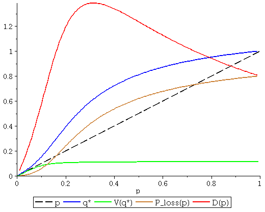
Figure 1: The case $K=1$, $\kappa=\sigma^{2}=0$, $C=4$. Data rate $p$, busy-link probability $q^{*}$, throughput $V_{T}(q^{*})$, loss probability $P_{\mathrm{loss}}(p,q^{*})$, latency $D(p)$ (gold).

By Lemma 4, for $K=1$ and $0<p<1$, the limiting busy link probability $q=q^{*}$ is the minimal solution of the balance equation $V_{T}(q)=p(1-q)/(1-p)$ and then the buffer size distribution is obtained as $\pi_{0}=(1-q)/(1-p)$, $\pi_{1}=(q-p)/(1-p)$. With the coverage probability in (23) this is a second order equation with solution

$$q^{*}=(\sqrt{(1-Cp)^{2}+4Cp^{2}}-(1-Cp))/2Cp,$$

hence the throughput as a function of $p$ equals

$$V_{T}(q^{*})=\frac{1}{2C(1-p)}\Big{(}1+Cp-\sqrt{(1-Cp)^{2}+4Cp^{2}}\Big{)}.$$

The delay is

$$D(p)=\mathbb{E}_{\pi}[B]/p=\pi_{1}/p=(q^{*}-p)/p(1-p),$$

which may be compared with the loss probability $P_{\mathrm{loss}}(p,q^{*})=1-V_{T}(q^{*})/p$. Figure 1 for $K=1$ visualizes the busy link probability, the coverage probability, the latency, and the loss probability as functions of $p$, for fixed $T$, $\delta$ and $w$ such that $C_{T,\delta,w}=4$. The latency represents time in buffer per arrival of new data. Hence the decrease in latency $D(p)$ for large data rates $p$ does not reflect improved performance but is merely a consequence of larger losses while throughput quickly reaches the maximum level $V_{T}(1)=1/5$.

IV-B No loss, the case $K=\infty$

Again we study the explicit situation in (23) with $\kappa=0$ and $\sigma^{2}=0$. For the no-loss model with given $w$ and $\delta$, and a fixed threshold $T$, there is a critical probability $p_{c}=p_{c}(T)$ such that for $0<p\leq p_{c}$, the balance equation, $V_{T}(q)=p$, has a uniqe solution $q^{*}$, $p<q^{*}\leq 1$, given by

$$q^{*}=\frac{p}{1-Cp},\quad p\leq p_{c}=\frac{1}{1+C}.$$

Equivalently, for fixed $p$ there is a critical threshold parameter $T_{\mathrm{max}}$ such that, if

$$T\leq T_{\mathrm{max}}=\sup\Big{\{}y:yK_{\delta}(1/y)<\frac{1}{w}\Big{(}\frac{1}{p}-1\Big{)}\Big{\}}^{\delta},$$

then again the balance equation has the unique solution $q^{*}=p/(1-Cp)$. The range of $T$-values is well-defined since the function $y\mapsto yK_{\delta}(1/y)$ is increasing. The buffer size has the geometric distribution

$$\mathbb{P}(B=k)=\pi_{k}=b^{k}(1-b),\;k\geq 0,\quad b=\frac{Cp^{2}}{(1-Cp)(1-p)}$$

and the delay is

$$D(p)=\mathbb{E}_{\pi}(B)/p=Cp/(1-p(1+C)),\quad p<p_{c}.$$

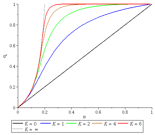
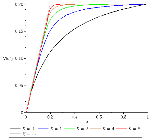
Figure 2: The case $\kappa=0$, $\sigma^{2}=0$. Critical arrival probability $p_{c}=1/5$. Upper panel: Busy link probabability $q^{*}$ as function of $p$ for varying buffer size $K$. Lower panel: Coverage probability $V_{T}(q^{*})$ for varying $K$.

IV-C Loss and delay as functions of buffer size $K$, $\kappa=\sigma^{2}=0$

To study how the loss and delay indicators change with buffer size $K$ it is convenient to continue with the reference case $\kappa=\sigma^{2}=0$. We have discussed the solutions $q^{*}$ and $V(q^{*})$ for $K=0$, $K=1$, and $K=\infty$. For $K=2,4,8$, additional numerical solutions are displayed graphically in Figure 2. The parameter $C=4$ is an arbitrary choice.

The corresponding loss probability $P_{\mathrm{loss}}(p,q^{*})$ and the buffer delay $D(p)$ are shown together in Figure 3, upper panel. To reveal more detail, these graphs have a logarithmic scale and focus on the most relevant parameter values $p$ not too far from $p_{c}=1/6$, which is the upper bound for the infinite buffer case.

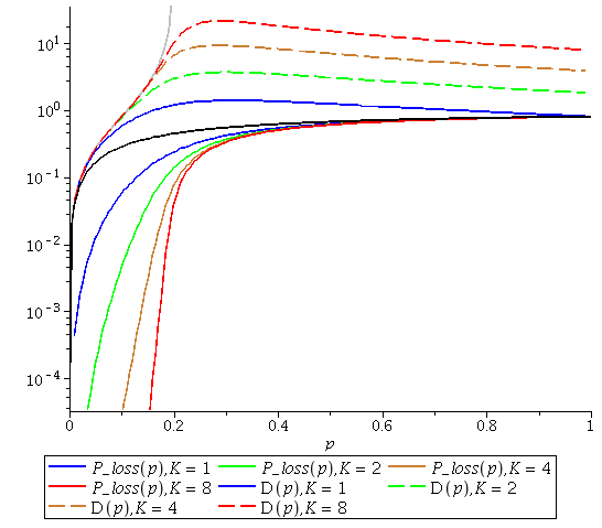
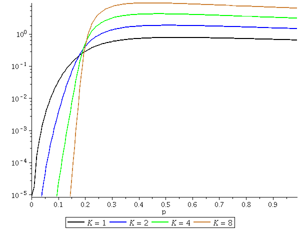
Figure 3: Upper panel: Logarithmic plots of loss probability (solid lines) and delay (dashed lines). Lower panel: Logarithmic plots of the loss-delay product.

The graphs confirm intuition that large buffer size favors reliability at the cost of latency and lead us to consider the trade-off between reliability and latency in the system subject to a given data rate. For $p$ well below $p_{c}$ it is seen that the loss probability is decreasing and hence the system is increasingly reliable with larger $K$, while latency as encoded by the buffer delay is still kept at reasonable levels. For $p$ near or above $p_{c}$, on the other hand, the delay builds up with increasing $K$ while the gain in smaller loss becomes less pronounced. These insights suggest that the loss-delay product

$$LD(p)=(1-V_{T}(p,q^{*})/p)\cdot D(p),\quad 0<p<1,$$

is a potentially relevant performance measure. Indeed, Figure 3, lower panel, displayed in logarithmic scale indicates a clear shift in $LD$-performance around the critical $p_{c}$. Large buffer size is preferred at lower traffic intensities but quickly turns counter-productive as soon as the system is subject to heavier data rates $p$ ranging above $p_{c}$.

In principle it is now possible to analyze a network with specified loss and delay requirements. Given network parameters $w$, $T$ and $\delta$, suppose we fix a maximal loss probability $L_{\mathrm{max}}$ and maximal average delay $D_{\mathrm{max}}$. Assuming we know that the network is operating at maximal data rate $p_{0}$, find for which buffer size values $K$ it holds that $P_{\mathrm{loss}}(p,q^{*})\leq L_{\mathrm{max}}$ and $D(p)\leq D_{\mathrm{max}}$, for all $p\leq p_{0}$. If there is a range of such $K$-values we are free to pick a prefered $K$ perhaps based on additional priorities for loss versus delay. If there is no such $K$ the desired loss-delay requirements are not viable for the system. Figure 4 provides a display. For example, with $p_{0}=0.09$ then for $D_{\mathrm{max}}=6$ we find $K<10$ and for $L_{\mathrm{max}}=0.03$ we find $K>3$. So for $4\leq K\leq 9$ both of the loss and delay criteria are fulfilled for every $p<p_{0}=0.09$.

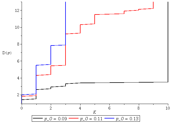
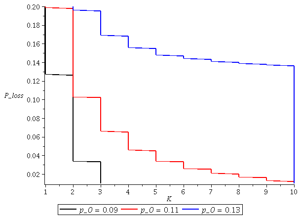
Figure 4: Choice of buffer size $K$ to provide preset loss and delay criteria

IV-D More realistic scenarios, $\sigma^{2}>0$ and/or $\kappa>0$

Moving away from the simplest coverage probability function $V_{T}(q)=q/(1+Cq)$, we consider briefly the case (22) with unbounded path loss ($\kappa=0$) but nonzero deterministic noise $\sigma^{2}>0$ and the general coverage probability for bounded path loss function, $\kappa>0$, derived in Lemma 2. The display in Figure 5 shows the shape of $V_{T}(q)$ as a function of the busy link probability $q$, for various combinations of $\sigma^{2}$ and $\kappa$, and other parameters fixed at $\mu=T=1$, $\delta=2$, $w=10$. The feature that stands out is that for $\kappa>0$, $V_{T}(q)$ may no longer be an increasing function of $q$. As a consequence the balance equation (21) may have more than one solution, noting that the properties in Theorem 1 refer to the minimal solution.

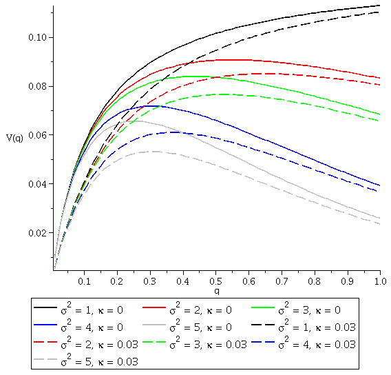
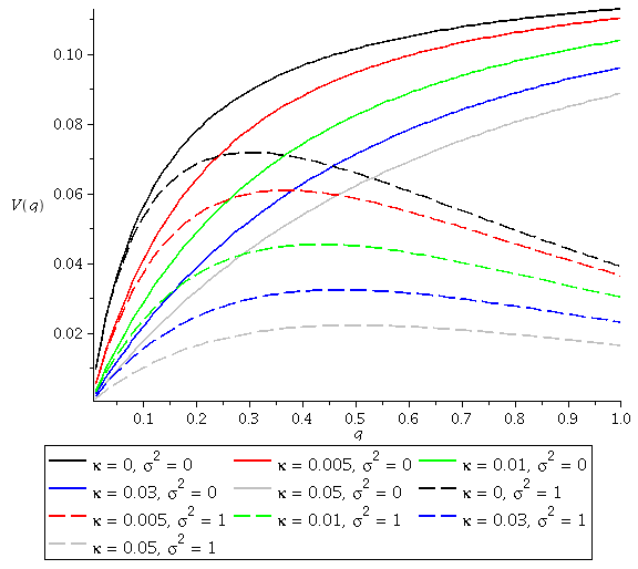
Figure 5: The coverage probability function $V_{T}(q)$ for various choices of parameters $\kappa$ and $\sigma$.

Finally, given $K$, solving iteratively for a minimal solution $q^{*}$, we obtain an approximation of the throughput $V_{T}(q^{*})$ as a function of the external data rate $p$. The throughput is reduced in comparison with the unbounded case $\kappa=0$, as indicated in Figure 6.

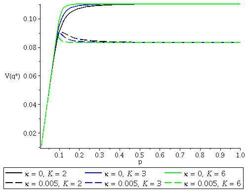
Figure 6: Comparison of throughput, singular attenuation $\kappa=0$, bounded attenuation $\kappa=0.005$.

References

- [AAB2018] A. AlAmmouri, J. G. Andrews and F. Baccelli, Asymptotic Analysis of Area Spectral Efficiency in Dense Cellular Networks. 2018 IEEE International Symposium on Information Theory (ISIT), Vail, CO, USA, 2018, pp. 56-60.
- [ABG2011] J.G. Andrews, F. Baccelli, R.K. Ganti, A tractable approach to coverage and rate in cellular networks. IEEE Transactions on Communications (2011) 59:11 3122-3134.
- [B2022] F. Baccelli, Stationary queues in space and time. Queueing Systems (2022) 100: 501-503.
- [BB2009] F. Baccelli, B. B. Blaszczyszyn, Stochastic Geometry and Wireless Networks: Volume 1 Theory. Foundations and Trends in Networking, 3:3-4 (2009) 249-449.
- [BDP2018] M. Bennis, M. Debbah, H.V. Poor, Ultrareliable and low-latency wireless communication: tail, risk, and scale. Proceedings of the IEEE (2018) 106:10, 1834-1853.
- [B1999] P. Brémaud, Markov Chains: Gibbs Fields, Monte Carlo Simulation and Queues. Springer-Verlag, New York, NY, 1999.
- [FZ1996] Foss, S.G., Zuyev, S.A.: On a Voronoi aggregative process related to a bivariate Poisson process. Adv. Appl. Probab. 28:4, 965–981 (1996).
- [GWF2016] R.F. Guiazon, K-K. Wong, M. Fitch, Coverage probability of cellular networks using interference alignment under imperfect CSI. D6igial Communications and Networks 2 (2016) 162-166.
- [H2012] Haenggi, M. (2012). Stochastic Geometry for Wireless Networks. Cambridge: Cambridge University Press. doi:10.1017/CBO9781139043816
- [IHV1998] J. Ilow, D. Hatzinakos, and A.N. Venetsanopoulos, Performance of FH SS radio networks with interference modeled as a mixture of Gaussian and -stable noise. IEEE Trans. on Communications 46, 509-520, 1998.
- [IM1976] D.L. Isaacson, R.W. Madsen, Markov Chains Theory and Applications. John Wiley & Sons, Inc., New York, NY, 1976.
- [K2002] I. Kaj, Stochastic modeling in broadband communications systems. SIAM Monographs in Mathematical Modeling and Computation 8. SIAM, Philadelphia, PH, 2002.
- [LPH2018] H. Lee, Y Park, and D. Hong, Resource split full duplex to mitigate inter-cell interference in ultra-dense small cell networks. In IEEE Access, vol. 6, pp. 37653-37664, 2018.
- [MK2022] T. Morozova, I. Kaj, Analysis of a typical cell in the uplink cellular network model using stochastic simulation. In proceedings of IEEE 2nd Conference on Information Technology and Data Science, CITDS 2022, Debrecen, Hungary, July 2022.
- [NDA2013] T.D. Novlan, H.S. Dhillon and J.G. Andrews, Analytical modeling of uplink cellular networks. IEEE Transactions on Wireless Communications !2:6 (2013) 2669–2679.
- [NMH2014] G. Nigam, P. Minero and M. Haenggi, Cooperative retransmission in heterogeneous cellular networks. 2014 IEEE Global Communications Conference, Austin, TX, USA, 2014, pp. 1528-1533.
- [SB2017] A. Sankararaman and F. Baccelli, Spatial Birth-Death Wireless Networks. IEEE Transactions on Information Theory, 63:6, pp. 3964-3982, 2017.
- [S1992] E.S. Sousa, Performance of a spread spectrum packet radio network link in a Poisson field of interferers. IEEE Trans. Inf. Theory 38, 1743-1754, 1992.
- [SKMC2013] D. Stoyan, W.S. Kendall, J. Mecke, S.N. Chiu, Stochastic Geometry and its Application, Third Ed. John Wiley & Sons, Ltd, Chichester UK, 2013.
- [TK1984] H. Takagi, L. Kleinrock, Optimal transmission ranges for randomly distributed packet radio terminals. IEEE Transactions on Communications 32: 3, 246-257, 1984.
- [YP] X. Yang, A.P. Petropulu, Co-channel interference modeling and analysis in a Poisson field of interferers in wireless communications. IEEE Trans. Signal Proc. 51, 64-76, 2003.
- [YLQ2016] H. H. Yang, J. Lee, and T. Q. S. Quek, Heterogeneous Cellular Network With Energy Harvesting-Based D2D Communication. IEEE Transactions on Wireless Communications, 15:2, 1406-1419, 2016.
- [YQ2018] H. H. Yang, T. Q. S. Quek, SIR coverage analysis in cellular networks with temporal traffic: a stochastic geometry approach. arXiv:1801.09888v1 [cs.IT]