Low-Confidence Samples Mining for Semi-supervised Object Detection

Abstract

Reliable pseudo-labels from unlabeled data play a key role in semi-supervised object detection (SSOD). However, the state-of-the-art SSOD methods all rely on pseudo-labels with high confidence, which ignore valuable pseudo-labels with lower confidence. Additionally, the insufficient excavation for unlabeled data results in an excessively low recall rate thus hurting the network training. In this paper, we propose a novel Low-confidence Samples Mining (LSM) method to utilize low-confidence pseudo-labels efficiently. Specifically, we develop an additional pseudo information mining (PIM) branch on account of low-resolution feature maps to extract reliable large-area instances, the IoUs of which are higher than small-area ones. Owing to the complementary predictions between PIM and the main branch, we further design self-distillation (SD) to compensate for both in a mutually-learning manner. Meanwhile, the extensibility of the above approaches enables our LSM to apply to Faster-RCNN and Deformable-DETR respectively. On the MS-COCO benchmark, our method achieves 3.54% mAP improvement over state-of-the-art methods under 5% labeling ratios.

1 Introduction

Deep neural networks Liu et al. (2017); Kim and Lee (2020) have achieved remarkable progress in the area of object detection. As model complexity increases, a large amount of precisely annotated data is required to train deep networks. To address this need, large-scale object datasets such as MS-COCO Lin et al. (2014) and Objects365 Shao et al. (2019) have been proposed in the community. Nevertheless, the process of annotation can be prohibitively expensive for real-world applications.

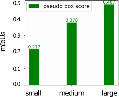
(a)

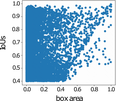
(b)

Figure 1: (a) Illustration of the mean IoU for pseudo-labels with three different size intervals (small:[0, 32$\times$32], medium:[32$\times$32, 96$\times$96], large:[96$\times$96, $+\infty$]). (b) IoU versus the box area for pseudo-labels.

Recently, semi-supervised object detection (SSOD) has gained attention in the computer vision community Liu et al. (2021); Zhou et al. (2021); Xu et al. (2021), as it only requires a small amount of annotated data. Most SSOD approaches follow the mean teacher paradigm Tarvainen and Valpola (2017), which trains a teacher and student model in a mutually beneficial manner. Pioneering approaches such as UBteacher Liu et al. (2021) and its variants Zhang et al. (2022); Chen et al. (2022a) improve detector performance from the perspective of classificatory balance. To further boost performance, SoftTeacher Xu et al. (2021) has been proposed, but these approaches do not consider the detailed distribution of pseudo-labels, which contain the box and category. Recalling previous works, it is apparent that there exists a significant gap in detection performance for boxes of different scales. This observation motivates the following question: Whether there exist differences in the confidence distribution of pseudo-labels between boxes of different scales?

To address this question, we conducted extensive experiments to explore the relationship between the confidence distribution and the scale of pseudo-labels. Initially, we trained a vanilla Faster-RCNN detector Ren et al. (2015) using all the labeled COCO training data. Subsequently, we generated pseudo-labels for the COCO validation set images. Following the methodology of prior works He et al. (2017); Cheng et al. (2020), we computed the IoUs (Intersection-over-Union) between the boxes in pseudo-labels and ground-truths with the same category, and we utilized these values to assess the quality of the pseudo-labels. Figure 1 illustrates the IoU distribution for pseudo-labels of different scales. Figure 1(a) shows that the pseudo-label quality is positively associated with the box’s scale. As the pseudo-label boxes increase in size, there are more pseudo-labels with high quality (Figure 1(b)), which will provide more precise box and category information for SSOD. Figure 2 visually depicts the pseudo-labels at various scales to qualitatively compare the differences in the confidence distribution of generated pseudo-labels with different scales. We observe that the pseudo-label of bus in Figure 2(b) (i.e., the large pink box with a classification score of $0.72$) is accurate, while the pseudo-label of toilet with a higher score but smaller area (the blue box surrounded by red dotted lines in Figure 2(a)) is incorrect. Intuitively, under the same confidence score, the detector tends to make more accurate predictions for larger-area samples than small-area ones. Hence, leveraging the scale information to exploit low-confidence pseudo-boxes adequately is a valuable technique.

Based on these observations, we have designed a novel training procedure for semi-supervised object detection (SSOD) called Low-confidence Sample Mining (LSM). The direct approach of adding large-area pseudo-labels with low confidence has shown limited improvement (as discussed in Section 5.1). Therefore, we propose leveraging low-resolution feature maps to learn reliable large-area candidate boxes, which is more suitable for large-area object training Singh et al. (2018); Li et al. (2019). Specifically, LSM introduces an additional branch called pseudo information mining (PIM) for self-learning low-confidence pseudo-labels. PIM downsamples the original image through a feature pyramid network (FPN) to obtain lower resolution feature maps. A lower threshold is set as DDT Zheng et al. (2022) to allow more pseudo-labels to participate in PIM training and help dig hidden credible low-confidence samples. Since scale information PIM uses can be produced in both Faster-RCNN and Deformable-DETR (DDETR) Zhu et al. (2021), it is natural to introduce DDETR into SSOD. During the joint training process of the main and PIM branches, we have observed that the candidate boxes learned by both branches have certain complementarity (see Section 5.3). To achieve mutual learning between these two branches, we introduce a self-distillation (SD) module. SD uses the prediction of PIM for low-confidence candidate boxes to supervise the main branch training, and calculates $\mathcal{KL}$ divergence loss between classificatory predictions from the main and PIM branches.

Under the same setting as mean teacher framework Liu et al. (2021); Xu et al. (2021), our method surpasses the previous state-of-the-arts by significant margins. Especially in the only $5\%$ labeled MS-COCO Lin et al. (2014), LSM achieves $3.54\%$ mAP improvement over state-of-the-arts. Furthermore, we find that mean teacher paradigm performances are below baseline on noisy unlabeled data (ImageNet Deng et al. (2009)). To verify the learning ability of LSM on more-noisy unlabeled data, we conduct a cross-domain task and introduce DDETR baseline into SSOD. Particularly, our method also outperforms DDETR Zhu et al. (2021) by $1.3\%$ mAP in the cross-domain setting.

The contributions of this paper are listed as follows:

• We explore the differences in confidence distribution for pseudo-labels between different scales. Moreover, we observe the positive correlation between pseudo-labels area and IoUs in SSOD and inspire the use of clean low-confidence boxes from a scale perspective. These observations provide a new direction to improve SSOD.

• Based on the above observations, we propose LSM, which uses PIM and SD to exploit clean low-confidence pseudo-labels from low-resolution feature maps efficiently. Extensive experiments are also performed on both Faster-RCNN and DDETR, which demonstrates that LSM does not rely on specific model components.

• We introduce DDETR into SSOD and use ImageNet Deng et al. (2009) as unlabeled data to conduct the cross-domain task, which indicates the excellent denoise capability of LSM.

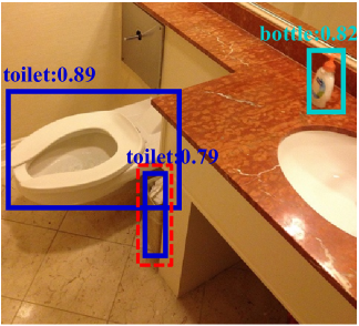
(a)

(b)

Figure 2: Illustration of pseudo-labels with boundary box, category and classification score. The incorrect pseudo-label (the toilet box in bottom) in (a) has a higher classification score than the correct pseudo-label (bus box) in (b).

2 Related Work

2.1 Semi-Supervised Learning

Semi-supervised learning constitutes a fundamental research area within the domain of deep learning. The most prevalent semi-supervised learning approaches are realized through consistency regularization Izmailov et al. (2018); Sajjadi et al. (2016); Kim et al. (2022); Xie et al. (2020a) and pseudo-labeling. Pseudo-labeling Sohn et al. (2020a); Berthelot et al. (2019); Xie et al. (2020b) involves appending predictions to the unlabeled data during the training process, utilizing a teacher model to assist in this task. Consequently, high-confidence predictions are selected as supervisory signals, which serve to enhance model training effectively.

2.2 Semi-Supervised Object Detection

The methodologies of semi-supervised object detection (SSOD) primarily stem from semi-supervised learning approaches. STAC Sohn et al. (2020b) is the first to apply pseudo-labeling and consistency learning to SSOD. It generates pseudo-labels for unlabeled data utilizing a pre-trained model, and subsequently trains a student model with strongly augmented unlabeled images. The mean teacher paradigm Liu et al. (2021); Zhou et al. (2021); Xu et al. (2021) maintains a teacher model for online pseudo-labeling, acquiring reliable pseudo-labels for student model training through a high threshold. However, due to the empirical nature of this threshold, numerous dependable supervisory signals are discarded. Dynamic threshold strategies Li et al. (2022b) seek to obtain a higher quantity of high-confidence supervisory samples by employing a variable threshold.

However, none of the above methods consider the hidden available low-confidence samples. Based on this, recent methods have made efforts in low-confidence samples learning.  Zheng et al. (2022) equips vanilla detector framework with the bypass head to learn pseudo-labels with a lower threshold.  Wang et al. (2022) takes the sum of Top-K probability predictions as the selection basis to expand learning samples. Nevertheless, they all lack further mining that refer to credible information in low-confidence samples and similarly take the incorrect pseudo-labels into training, e.g., the mistaken toilet box in Figure 2(a) will be retained in the above-both methods. Furthermore, the object detector based on transformer has shown powerful performance in recent years.  Carion et al. (2020); Zhu et al. (2021) utilize the attention mechanism to get a larger receptive field on the feature map and apply bipartite graph matching to implement end-to-end training. Limited by mean teacher framework, many SSOD methods Chen et al. (2022a, b) cannot be directly applied to transformer structure. This hinders the application of Deformable-DETR (DDETR) in SSOD. Owing to the multi-scale feature maps LSM used can be produced by both DDETR and Faster-RCNN. Our work can be applied in DDETR effortlessly.

2.3 Multi-Scale Invariant Learning

Multi-scale invariant learning plays a vital role in object detection (OD) by facilitating the learning of objects across different scales. Singh et al. (2018) accelerates multi-scale training by sampling low-resolution chips from a multi-scale image pyramid. Li et al. (2019) employs convolutions with three distinct dilation rates to extract features from objects of varying sizes. Both methods demonstrate remarkable performance in multi-scale learning. Inspired by multi-scale training, our proposed PIM utilizes downsampling and a feature pyramid network (FPN) to generate lower-resolution feature maps for learning large-area objects.

In fact, Li et al. (2022a) and Guo et al. (2022) incorporate multi-scale label consistency into the mean teacher framework, striving to learn consistent representations across diverse scales. Although these approaches feature a branch for aligning dense features at different scales, which assists in mining scale-equivariant background features, they still rely on high-confidence pseudo-labels as the training target between the two branches. While our LSM method will utilize supplementary foreground proposals from low-confidence pseudo-labels.

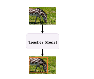
(a) generation of pseudo-labels

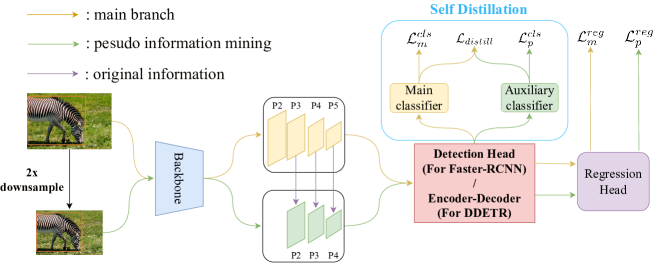
(b) low-confidence samples mining (LSM)

Figure 3: An overview of our training method. (a) represents the generation of pseudo-labels. (b) illustrates the pipeline of LSM. The yellow line is the main branch following mean teacher framework and the green line is the forward procedure of PIM. The purple line is original information reused by PIM from the main branch. It refers to the proposals generated by the region proposal network (RPN) in Faster-RCNN, and indexes of bipartite graph matching results from in DDETR. The detector is equipped with self-distillation (SD) to learn complementary predictions from two branches.

3 Methodology

3.1 Problem Definition

Semi-supervised object detection aims to use a large amount of unlabeled data to improve model performance, where a small labeled dataset $D^{l}=\{I_{i}^{l},Y_{i}^{l}\}_{i=1}^{N^{l}}$ and a large unlabeled dataset $D^{u}=\{I_{i}^{u}\}_{i=1}^{N^{u}}$ are available. $N^{l},N^{u}$ presents the number of labeled, unlabeled data. $Y_{i}$ contains object information of image $I_{i}$, including bounding box $\{x_{j},y_{j},w_{j},h_{j}\}_{j=1}^{N^{I}_{i}}$ and category $\{c_{j}\}_{j=1}^{N^{I}_{i}}$. ${N^{I}_{i}}$ presents the number of objects in the $i$th picture.

3.2 Preliminary: Mean Teacher Framework

In the regime of SSOD, this study takes two-stage methods based on the mean teacher paradigm Tarvainen and Valpola (2017) as the baseline. Following previous works, we first train the student model on labeled data and then copy the parameters of the student model to the teacher model. The student model accepts both labeled data and unlabeled data, of which supervision signals come from the teacher model’s predictions. The loss function of SSOD can be summarized as supervised loss $\mathcal{L}_{s}$ and unsupervised loss $\mathcal{L}_{u}$,

$$\mathcal{L} =\mathcal{L}_{s}+\lambda_{u}\mathcal{L}_{u},$$ (1)

$$\mathcal{L}_{s} =\mathcal{L}_{cls}(I^{s},Y^{s})+\mathcal{L}_{reg}(I^{s},Y^{s}),$$

$$\mathcal{L}_{u} =\mathcal{L}_{cls}(I^{u},\hat{Y}^{u})+\mathcal{L}_{reg}(I^{u},\hat{Y}^{u}).$$

Among them, $\mathcal{L}_{cls}$ represents classification loss, and $\mathcal{L}_{reg}$ represents regression loss. $\hat{Y}^{u}$ represents the pseudo-labels generated by the teacher model, and $\lambda_{u}$ is the weight of unsupervised loss. During per iteration, the student model will update the teacher model with its own parameters in the way of exponential moving average (EMA) and generate cleaner pseudo-labels.

$$\theta_{s} \leftarrow\theta_{s}+\frac{\partial\mathcal{L}}{\partial\theta_{s}},$$ (2)

$$\theta_{t} \leftarrow\lambda_{e}\theta_{t}+(1-\lambda_{e})\theta_{s},$$

where $\theta_{s},\theta_{t}$ represents the parameters of the student, teacher model, and $\lambda_{e}$ represents the ratio of parameter updates.

3.3 Low-confidence Samples Mining (LSM)

In this section, we introduce the LSM method. The reliable latent low-confidence pseudo-labels are mined adequately through pseudo information mining (PIM) and self-distillation (SD). The confidence in this section later refers to the classification score.

3.3.1 Overview

We introduce the whole pipeline of our LSM method in Figure 3 and LSM is applied in the student model after burn-in under the mean teacher framework. First of all, the teacher model trained on a small amount of labeled data $D^{l}$ is utilized to produce pseudo-labels for $D^{u}$. Regarding the hybrid training of ground-truths and pseudo-labels, LSM consists of the main branch and pseudo information mining (PIM) for low-confidence pseudo-labels learning. As shown in the yellow line in Figure 3(b), the main branch receives the original feature maps group and leverages pseudo-labels with a high threshold $t$. While the PIM receives downsampling feature maps to learn low-confidence pseudo-labels. The total loss of LSM can be formulated as follow,

$$\mathcal{L}_{total}=\mathcal{L}_{m}^{s}+ \lambda_{u}(\mathcal{L}_{m}^{u}+\mathcal{L}_{p}^{u}+\mathcal{L}_{distill}),$$ (3)

where $\mathcal{L}_{m}^{s}$ and $\mathcal{L}_{m}^{u}$ refer to supervised loss and unsupervised loss from the main branch, which are the same loss from the mean teacher paradigm. While $\mathcal{L}_{p}^{u}$ represents unsupervised loss from PIM. $\mathcal{L}_{distill}$ means distillation loss under the self-distillation (SD) strategy.

3.3.2 Pseudo Information Mining (PIM)

Motivated by the positive correlation between the area and IoUs of pseudo boxes observed in Figure 1, we aim to mine reliable pseudo-labels from a scale perspective. As shown in Section 5.1, directly incorporating large-area pseudo-labels (area $>96\times 96$) with a lower-confidence threshold of $0.5$ into training yields some improvement. However, utilizing an area threshold of ($96\times 96$) as an empirical parameter is inappropriate for defining large-area boxes. Since detectors tend to learn large objects from low-resolution feature maps, we are inspired to extract valuable large-area pseudo-labels from small-scale images. Consequently, we design PIM from a multi-scale standpoint to learn reliable large-area pseudo-labels with low confidence. The green line in Figure 3(b) depicts the forward procedure of PIM.

Initially, PIM downsamples the original image by a ratio of 0.5 (both width and height are reduced to half of their original sizes), and then inputs the downsampled image into the backbone. A Feature Pyramid Network (FPN) generates a series of small-scale feature maps from the downsampled image, referred to as downsampling feature maps. The $i$th downsampling feature map shares the same size as the ($i+1$)th original feature map. Subsequently, PIM establishes a lower threshold $\alpha$ to include more pseudo-labels in PIM training, fostering the extraction of diverse information by the detector. As downsampling feature maps possess lower resolution, the box features extracted from the detector in PIM are inclined to learn credible large-area candidate boxes. These box features from PIM are then fed into an auxiliary classifier and regression head to compute $\mathcal{L}_{p}^{cls}$ and $\mathcal{L}_{p}^{reg}$. PIM ensures that the detector learns valuable information from low-confidence pseudo-labels, while the detector’s bias towards large-area pseudo-labels on low-resolution feature maps mitigates the adverse impact of noisy small-area pseudo-labels. Moreover, we decrease the loss weight of PIM to further minimize the influence of noisy pseudo-labels.

To reduce the computational load during forward propagation, PIM reuses the original proposals from the main branch (purple line in Figure 3; more details about original information are provided in the supplementary material). Notably, PIM employs $P_{2},P_{3},P_{4}$ feature maps to align the $P_{3},P_{4},P_{5}$ feature maps from the main branch in a shift alignment manner. As a result, the main branch can share proposals generated by the Region Proposal Network (RPN) with PIM. The loss of PIM can be formulated as follows:

$$\mathcal{L}_{m}^{s} =\mathcal{L}^{cls}_{m}(F_{main}(E(I_{m}^{s})),Y^{s})+\mathcal{L}^{reg}_{m}(R(E(I_{m}^{s})),Y^{s})$$ (4)

$$\mathcal{L}_{m}^{u} =\mathbb{I}_{\{\hat{Y}_{score}^{u}>t\}}[\mathcal{L}^{cls}_{m}(F_{main}(E(I_{m}^{u})),\hat{Y}^{u})$$ (5)

$$+\mathcal{L}^{reg}_{m}(R(E(I_{m}^{u})),\hat{Y}^{u})].$$

$$\mathcal{L}_{p}^{u} =\mathbb{I}_{\{\hat{Y}_{score}^{u}>\alpha\}}[\mathcal{L}^{cls}_{p}(F_{aux}(E(I_{p}^{u})),\hat{Y}^{u})$$ (6)

$$+\mathcal{L}^{reg}_{p}(R(E(I^{u}_{p})),\hat{Y}^{u})].$$

Among them, $t$ is the filtering threshold of the main branch. And $\alpha$ is the filtering threshold of PIM, which is lower than $t$. $E$ is the feature extractor, and $R$ is the regression head shared with the main branch and PIM. $F_{main}$ is the main classifier, while $F_{aux}$ is the auxiliary classifier. At the same time, $\mathcal{L}_{p}^{u}$ and $\mathcal{L}_{m}^{u}$ also indicate that the model is forced to learn consistent representations under different-scale features in score interval $[t,\infty]$ to enhance the robustness of the detector model. Eq. 6 indicates that PIM can acquire more valuable pseudo boxes from the low-confidence samples due to a lower threshold filtering strategy, especially in Section 4.3 we show that this method can improve recall rate well compared to previous state-of-the-art methods.

PIM has certain similarities with multi-scale label consistency (MLC) Li et al. (2022a). However, MLC aims to improve the robustness of the model via learning the same pseudo-labels from different-scale feature maps, which also ignores low-confidence pseudo boxes. Thereby it interferes the further learning on pseudo-labels. The convincing experimental results are presented in Table 4.

3.3.3 Self Distillation (SD)

LSM processes the box predictions from two branches by feeding them into the main classifier and auxiliary classifier, respectively. Due to the complementary predictions observed from the auxiliary classifier, the detector employs self-distillation to incorporate the knowledge of low-confidence bounding boxes learned by the auxiliary classifier into the main classifier. Specifically, we generate categorical predictions using an auxiliary classifier for bounding boxes with confidences in the [$\alpha$, $t$] range. Then, we employ the categorical predictions generated by the main classifier, with confidences in the same interval, to fit the corresponding predictions produced by the auxiliary classifier. The distillation loss is expressed as:

$$\mathcal{L}_{distill}=\mathbb{I}_{\{\alpha<\hat{y}^{u}_{score}<t\}}\mathcal{L}_{kl}(F_{main}E(I^{u}_{m}),F_{aux}E(I^{u}_{p})).$$ (7)

$\mathcal{L}_{kl}$ calculates the $\mathcal{KL}$ divergence between the output of the main and auxiliary classifiers. Threshold $t$ and $\alpha$ are the same as those set in Eq. 5 and Eq. 6. Regarding the categorical distribution of low-confidence candidate boxes, it is unsuitable to directly choose the category with maximum probability as the hard label due to noise interference. Moreover, some categories with high probability may also be potential labels for the candidate box. Therefore, SD aids the main branch in learning soft predictions from PIM. Additionally, although the auxiliary classifier learns external pseudo-labels, it is still affected by noisy labels. Leveraging the complementarity of dual classifiers, we do not detach the gradient for PIM in SD, allowing the main branch to supervise PIM in a mutually-learning manner. This approach not only ensures that the main classifier learns more pseudo-labels but also mitigates the impact of noisy labels on the auxiliary classifier.

3.3.4 LSM for Deformable-DETR (DDETR)

PIM, combined with SD, constitutes the LSM method. Since LSM does not rely on specific network components, it can be effectively transferred to DDETR. The only difference between Faster-RCNN and DDETR, both implemented with LSM, is the original proposals. The results of bipartite graph matching between box predictions from the main branch and pseudo-labels are reused in PIM, as depicted by the purple line in Figure 3(b). Due to memory limitations, we employ the STAC Sohn et al. (2020b) and pretrain-finetune training strategies for DDETR in the SSOD setting. Specifically, in the first stage, both strategies generate pseudo-labels for unlabeled data using a pre-trained model. In the second stage, STAC trains DDETR with a combination of labeled data and high-confidence unlabeled data, while pretrain-finetune first trains DDETR with unlabeled data and then finetunes it on labeled data. Notably, LSM can be applied in the second stage of both strategies.

In detail, we feed two stacks of original feature maps and low-resolution feature maps into the encoder to obtain two sets of reference points. Then, the object queries conduct cross attention with the reference points from the two sets, respectively, generating two groups of predictions from the two branches. The predictions from the two branches and the pseudo-labels in the two threshold intervals compute $\mathcal{L}_{m}^{u},\mathcal{L}_{p}^{u}$, respectively. Finally, the dual classifiers generate classification predictions to compute $\mathcal{L}_{distill}$. During the inference phase, only the main branch is used for forward computation, and the PIM branch is discarded.

	COCO-standard ($AP_{50:95}$)				COCO-additional
	$1\%$	$2\%$	$5\%$	$10\%$	$100\%$ ($AP_{50:95}$)
Supervised	$9.05\pm 0.16$	$12.70\pm 0.15$	$18.47\pm 0.22$	$23.86\pm 0.81$	$40.20$
CSD Jeong et al. (2019)	$10.51\pm 0.06$	$13.93\pm 0.12$	$18.63\pm 0.07$	$22.46\pm 0.08$	$38.82$
STAC Sohn et al. (2020b)	$13.97\pm 0.35$	$18.25\pm 0.25$	$24.38\pm 0.12$	$28.64\pm 0.21$	$39.21$
Humble Teacher Tang et al. (2021)	$16.96\pm 0.35$	$21.74\pm 0.24$	$27.70\pm 0.15$	$31.61\pm 0.28$	$42.17$
ISMT Yang et al. (2021)	$18.88\pm 0.74$	$22.43\pm 0.56$	$26.37\pm 0.24$	$30.53\pm 0.52$	$39.60$
Instant Teaching Zhou et al. (2021)	$18.05\pm 0.15$	$22.45\pm 0.15$	$26.75\pm 0.05$	$30.40\pm 0.05$	$40.20$
MUM Kim et al. (2022)	$21.88\pm 0.12$	$24.84\pm 0.10$	$28.52\pm 0.09$	$31.87\pm 0.30$	$42.11$
UBteacher Liu et al. (2021)	$20.75\pm 0.12$	$24.30\pm 0.07$	$28.27\pm 0.11$	$31.50\pm 0.10$	$41.30$
UBteacher + LSM	$\mathbb{23.95\pm 0.02}$	$\mathbb{26.60\pm 0.04}$	$\mathbb{31.97\pm 0.09}$	$\mathbb{34.75\pm 0.13}$	$\mathbb{43.23}$
SoftTeacher Xu et al. (2021)	$20.46\pm 0.39$	-	$30.74\pm 0.08$	$34.04\pm 0.14$	$44.50$
SoftTeacher + LSM	$\mathbb{23.76\pm 0.18}$	-	$\mathbb{33.47\pm 0.21}$	$\mathbb{36.14\pm 0.09}$	$\mathbb{45.70}$
PseCo Li et al. (2022a)	$22.43\pm 0.36$	$27.77\pm 0.18$	$32.50\pm 0.08$	$36.08\pm 0.24$	$46.10$
PseCo + LSM	$\mathbb{24.17\pm 0.21}$	$2\mathbb{8.96\pm 0.07}$	$\mathbb{34.21\pm 0.11}$	$\mathbb{37.33\pm 0.08}$	$\mathbb{47.01}$

Table 1: Comparison with the state-of-the-arts from different percentages of labeled MS-COCO. The margins of error are reported under 5 different random seeds. Where“-” means the corresponding result is not available.

	$AP_{50}$	${AP_{50:95}}$
supervised	$72.63$	$42.13$
STAC Sohn et al. (2020b)	$77.45$	$44.64$
UBteacher Liu et al. (2021)	$78.37$	$50.69$
Humble Teacher Tang et al. (2021)	$80.94$	$53.04$
UBteacher + LSM	$\mathbb{81.61}$	$\mathbb{54.90}$

Table 2: Comparison with the state-of-the-arts on VOC.

	COCO-ImageNet ($AP_{50:95}$)
	Step	mAP
STAC Sohn et al. (2020b)	$360$K iter	$36.47$
UBteacher Liu et al. (2021)	$360$K iter	$38.47$
UBteacher∗ (Ours)	$360$K iter	$\mathbb{39.87}$
Deformable-DETR (STAC)	$50$ epoch	$40.11$
Deformable-DETR∗(STAC)	$50$ epoch	$\mathbb{42.72}$
Deformable-DETRΩ Zhu et al. (2021)	$50$ epoch	$43.32$
Deformable-DETRΦ	$50$ epoch	$44.01$
Deformable-DETRΦ(LSM)	$50$ epoch	$\mathbb{45.34}$

Table 3: Comparison with the state-of-the-arts on COCO-ImageNet. Where “*” represents that the LSM is applied on the corresponding model and “$\Omega$” means that the model is only trained on train2017 in a fully-supervised manner. “$\Phi$” indicates that the model is pre-trained with $20\%$ ImageNet, and then finetuned with train2017. The last row represents that our method is solely applied in the pre-training stage.

	Data setting	Step	$AP_{50:95}$
UBteacher Liu et al. (2021)	$5\%$ COCO	$180$K iter	$28.27$
UBteacherΔ Li et al. (2022a)	$5\%$ COCO	$180$K iter	$30.06$
PIM (In UBteacher)	$5\%$ COCO	$180$K iter	$\mathbb{31.81}$
STAC Sohn et al. (2020b)	COCO-ImageNet	$360$K iter	$36.47$
STACΔ Li et al. (2022a)	COCO-ImageNet	$360$K iter	$36.77$
PIM (In STAC)	COCO-ImageNet	$360$K iter	$\mathbb{37.87}$
UBteacher Liu et al. (2021)	COCO-ImageNet	$360$K iter	$38.47$
UBteacherΔ Li et al. (2022a)	COCO-ImageNet	$360$K iter	$38.81$
PIM (In UBteacher)	COCO-ImageNet	$360$K iter	$\mathbb{39.87}$

Table 4: Comparison with Multi-scale Label Consistency (MLC). “$\Delta$” indicates that the model is trained using MLC.

4 Experiment

4.1 Datasets

In this section, we carry out extensive experiments to validate the effectiveness of LSM on the MS-COCO Lin et al. (2014), PASCAL VOC Everingham et al. (2010), and ImageNet Deng et al. (2009) benchmarks.

MS-COCO contains two training sets, the train2017 dataset with 118K labeled images and the unlabeled2017 dataset with 123K unlabeled images. Following previous methods, we conduct experiments under three settings: (1) COCO-standard: we sample 1%, 2%, 5%, and 10% of the images from train2017 as labeled data, while the rest are treated as unlabeled data. (2) COCO-additional: We use the full train2017 dataset as labeled data and the unlabeled2017 dataset as unlabeled data. (3) VOC: We use the VOC07-trainval as the labeled dataset and the VOC12-trainval as the unlabeled dataset. We evaluate the model on COCO-val2017 for (1)(2) and VOC07-test for (3).

In addition to these three traditional settings, we find that previous SSOD methods have not conducted cross-domain experiments on a more noisy unlabeled dataset. To demonstrate the denoising capacity of LSM-equipped Deformable-DETR on cross-domain tasks under SSOD settings, we introduce a fourth experimental setting: (4) COCO-ImageNet: We use the full train2017 dataset as labeled data and randomly choose 20% of ImageNet as noisy unlabeled data. The pseudo-labels for unlabeled data are predicted by the Faster-RCNN trained on the train2017 dataset.

4.2 Implementation Details

To be fair, we use Faster-RCNN as our base object detector as same as previous studies Liu et al. (2021); Xu et al. (2021). The weights of the backbone are initialized with ImageNet pre-trained model. For the main branch, we set pseudo boxes filtering threshold $t$ to $0.7$. While for LSM, which can have a higher tolerance for pseudo boxes, we set the threshold $\alpha$ to $0.5$. In all training settings, each of our training batches follows previous correspond works. For COCO-standard, the entire training steps are $180,000$, of which the first $20,000$ steps are used to pre-train the student model with labeled images. For COCO-additional, pre-training steps are $90,000$, and the whole training steps are $360,000$. For COCO-ImageNet, it takes the same training steps as COCO-additional due to the data size is close. In our experiments, strong data augmentation involves random jittering, gaussian noise, crop, and weak data augmentation involves random resize and flip. Moreover, we follow the existing work Liu et al. (2021); Xu et al. (2021) to set the above hyperparameters.

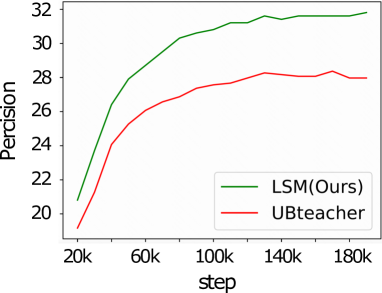
(a) 5% COCO Avg Recall

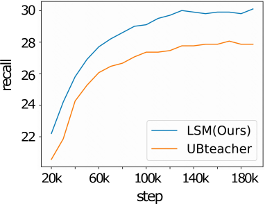
(b) 5% COCO Avg Precision

Figure 4: Comparison of the average recall and average precision curves for UBTeacher and LSM(ours) on 5% COCO-standard.

4.3 Results

4.3.1 COCO-standard

We first evaluate our method under the COCO-standard setting. As shown in Table 1, UBteacher Liu et al. (2021) equipped with LSM can perform better than previous work. When trained on $5\%$ COCO-standard, LSM outperforms the UBteacher by $3.54\%$ mAP. Even if LSM is applied to SoftTeacher (PseCo), it can also improve by $2.71\%$ ($1.47\%$) mAP on average in $1\%$, $5\%$ and $10\%$ labeled data. We attribute the success of model performance to the stronger ability to capture object boxes in LSM. As shown in Figure 4(a), under the setting of $5\%$ COCO-standard, the recall rate of LSM is higher than that of the UBteacher in the whole training stage, which means that after adding LSM, the model can better detect the previous missing boxes. Figure 4(b) indicates that the mAP metric of LSM is better than that of UBTeacher. Theoretically, LSM adds an extra branch to learn low-confidence pseudo-labels, and the downsampling operation biases the model to learn more clean large-area pseudo boxes thus extracting additional information.

4.3.2 COCO-additional

In this section, we verify LSM can be further improved when trained on large-scale labeled data with additional unlabeled data. As shown in Table 1, when LSM is applied to the UBTeacher, it can improve $1.93\%$ mAP compared to the UBTeacher baseline While LSM also achieves $1.2\%$ mAP improvement with applying in SoftTeacher baseline. These results indicate that our method achieves satisfactory improvement on large-scale unlabeled datasets.

4.3.3 VOC

We evaluate models on a balanced dataset VOC to demostrate the generalization of LSM. Table 2 provides the mAP results of CSD, STAC, UBteacher, Humble Teacher and our LSM-equipped UBteacher. Our method achieves $4.21\%$ mAP improvement compared with UBteacher baseline and $1.86\%$ mAP improvement compared with Humble teacher. Our method surpasses the other state-of-the-art results with a large margin. These results demonstrate that LSM can improve the existing SSOD consistently in various datasets.

4.3.4 COCO-ImageNet

To verify the effectiveness of LSM-equipped DDETR, we propose a new cross-domain setting: COCO-ImageNet. Considering that DDETR converges slowly, we use epochs as the unit in the training process.

As shown in Table 3 row 2, the detector reduces $1.73\%$ mAP compared to the fully supervised mode in UBteacher paradigm. While LSM demonstrates excellent denoise capability, with an improvement of $1.4\%$ mAP compared to the UBTeacher baseline. Furthermore, in the training mode of pretrain-finetune, we find that DDETR performs better ($0.7\%$ mAP) than the supervised baseline, which indicates that the pretrain-finetune mode can better utilize more noisy pseudo-labels. Moreover, after applying LSM to the pre-training stage of DDETR, we observe that the model can achieve a $1.3\%$ mAP improvement. This shows that LSM not only can be applied to Faster-RCNN and DDETR as a decoupling method but also has excellent learning ability in noisy labels.

4.3.5 Compared with Multi-scale Label Consistency (MLC)

The downsampling method used by our PIM follows the multi-scale label consistency method. MLC is widely used in object detection as an incremental method.However, existing methods force the model to learn a consistent representation of high-confidence pseido-labels between the two branches. PIM, on the other hand, equips the downsampling branch with a lower filtering threshold, to capture more information from pseudo-labels. To verify that our PIM outperforms the MLC method, we apply these two methods under two settings of $5\%$ COCO-standard and COCO-ImageNet, respectively.

As shown in Table 4, under the setting of $5\%$ COCO, applying the MLC on UBteacher can improve $1.79\%$ mAP, while applying PIM can improve $3.54\%$ mAP. In the COCO-ImageNet setting, we find that applying MLC on STAC brings a limited improvement ($0.3\%$ mAP) while applying the PIM can bring $1.4\%$ mAP improvement.

5 Ablation Study

5.1 Effects of Pseudo Information Mining Branch

PIM uses downsampling method to obtain three different-resolution feature maps of $P_{2}^{d}$, $P_{3}^{d}$, and $P_{4}^{d}$ generated by feature pyramid network (FPN). As shown in Table 5, we select multiple combinations from three feature maps to learn low-confidence samples. From row 2, the baseline has a certain improvement ($0.76\%$ mAP) through directly adding large-area pseudo-labels exceeding a lower threshold to the training. Whereas we find that using $P_{2}^{d}$, $P_{3}^{d}$, and $P_{4}^{d}$ simultaneously in the PIM, the model performs the best, $3.2\%$ mAP higher than the UBteacher baseline in row 6. As shown in row 3, if we only use the $P_{2}^{d}$, $P_{3}^{d}$, we find that the extra object information learned by the PIM is very limited, which is only $0.4\%$ mAP higher than the baseline. When we add the lower resolution feature map $P_{4}^{d}$ (as shown in row 4), we find that the performance will be significantly improved, which is $2.41\%$ mAP higher than the baseline. Through the comparison of the row 3 and the row 5 of Table 5, we can find that the combined detection of $P_{3}^{d}$ and $P_{4}^{d}$ on large objects is $3.54\%$ $AP_{L}$ higher than that of $P_{2}^{d}$ and $P_{3}^{d}$. This shows that using lower resolution feature maps for PIM can indeed better mine large objects with lower confidence.

	$P_{2}^{d}$	$P_{3}^{d}$	$P_{4}^{d}$	$AP_{50:95}$	$AP_{S}$	$AP_{M}$	$AP_{L}$
$1$				$20.75$	$9.21$	$21.73$	$27.32$
$2$				$21.41$	$9.23$	$22.45$	$28.13$
$3$	✓	✓		$21.15{(+0.4)}$	$9.10$	$22.63$	$27.87$
$4$	✓		✓	$23.16{(+2.41)}$	$11.36$	$25.73$	$30.91$
$5$		✓	✓	$23.24{(+2.49)}$	$11.48$	$25.88$	$\mathbb{31.41}$
$6$	✓	✓	✓	$\mathbb{23.95}{(+3.2)}$	$\mathbb{11.90}$	$\mathbb{26.83}$	$31.21$

Table 5: Ablation study on PIM under $1\%$ COCO-standard. The row 1 represents the UBteacher baseline without using $P_{2}^{d},P_{3}^{d},P_{4}^{d}$. The row 2 indicates that large objects exceeding a lower threshold ($t>0.5$, area $>96\times 96$) are added to the training of UBteacher baseline.

5.2 Effects of Filter Threshold

Threshold plays a key role in screening high-quality pseudo-labels. Figure 5 shows the performance of the model under $1\%$ COCO-standard at different thresholds. The red line represents the corresponding performance of the UBteacher after adjusting the threshold $t$. The blue line shows the corresponding performance of the LSM-equipped UBteacher after adjusting the threshold $\alpha$. For UBTeacher, it is difficult for the model to utilize the useful low-confidence pseudo-labels, and the performance of the model becomes worse as the threshold decreases. Moreover, it is difficult for the model to improve further after the threshold exceeds $0.6$. For LSM, the performance of the model reaches the highest $23.95\%$ mAP for $\alpha=0.5$. Therefore, our method can make sufficient use of pseudo-labels with low confidence (i.e., $\hat{Y}_{score}^{u}\in[0.5,0.7])$, which is not achieved by previous methods.

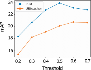
Figure 5: Ablation study on filtering threshold

5.3 Effects of Self-distillation

In this experiment, the original PIM and the PIM equipped with SD are compared. Table 6 shows the performance gain on the UBTeacher ($1\%$ COCO-standard setting) and DDETR models respectively. As can be seen, PIM+SD can improve $0.2\%$ (resp. $0.4\%$) mAP on UBTeacher (resp. DDETR) than PIM, which demonstrates the effectiveness of SD. As the PIM branch has learned external low-confidence pseudo-labels, the PIM branch would be complementary to the main branch. This complementarity is illustrated with more visual results in the supplementary material

	UB		DDETR
Method	PIM	PIM+SD	PIM	PIM+SD
$AP_{50:95}$	$34.55$	$\mathbb{34.75}$	$44.9$	$\mathbb{45.3}$

Table 6: Ablation study on self-distillation.

6 Conclusion

In this study, we dive into the problem of discarding numerous low-confidence samples. Motivated by the positive correlation between area and IoUs of pseudo boxes, we propose the LSM method consists of PIM and SD. As high-level feature maps is conductive to learn large candidate boxes, PIM utilizes downsampling method and a lower threshold to extract diverse information from low-confidence pseudo-labels. Moreover, LSM takes advantage of SD to make PIM and main branch in mutually-learning manner. Sufficient experiments on benchmark demonstrate the superiority of our method. At the same time, our method can be freely applied to DETR framework, and shows excellent denoise ability on the cross-domain task.

References

- Berthelot et al. [2019] David Berthelot, Nicholas Carlini, Ian Goodfellow, Nicolas Papernot, Avital Oliver, and Colin A Raffel. Mixmatch: a holistic approach to semi-supervised learning. In NeurIPS, volume 32, 2019.
- Carion et al. [2020] Nicolas Carion, Francisco Massa, Gabriel Synnaeve, Nicolas Usunier, Alexander Kirillov, and Sergey Zagoruyko. End-to-end object detection with transformers. In ECCV, pages 213–229, 2020.
- Chen et al. [2022a] Binbin Chen, Weijie Chen, Shicai Yang, Yunyi Xuan, Jie Song, Di Xie, Shiliang Pu, Mingli Song, and Yueting Zhuang. Label matching semi-supervised object detection. In CVPR, pages 14381–14390, 2022.
- Chen et al. [2022b] Binghui Chen, Pengyu Li, Xiang Chen, Biao Wang, Lei Zhang, and Xian-Sheng Hua. Dense learning based semi-supervised object detection. In CVPR, pages 4815–4824, 2022.
- Cheng et al. [2020] Tianheng Cheng, Xinggang Wang, Lichao Huang, and Wenyu Liu. Boundary-preserving mask r-cnn. In ECCV, pages 660–676, 2020.
- Deng et al. [2009] Jia Deng, Wei Dong, Richard Socher, Li-Jia Li, Kai Li, and Li Fei-Fei. {ImageNet}: a large-scale hierarchical image database. In CVPR, pages 248–255, 2009.
- Everingham et al. [2010] Mark Everingham, Luc Van Gool, Christopher KI Williams, John Winn, and Andrew Zisserman. The pascal visual object classes (voc) challenge. pages 303–338, 2010.
- Guo et al. [2022] Qiushan Guo, Yao Mu, Jianyu Chen, Tianqi Wang, Yizhou Yu, and Ping Luo. Scale-equivalent distillation for semi-supervised object detection. In CVPR, pages 14522–14531, 2022.
- He et al. [2017] Kaiming He, Georgia Gkioxari, Piotr Dollár, and Ross Girshick. Mask r-cnn. In ICCV, pages 2961–2969, 2017.
- Izmailov et al. [2018] Pavel Izmailov, Dmitrii Podoprikhin, Timur Garipov, Dmitry Vetrov, and Andrew Gordon Wilson. Averaging weights leads to wider optima and better generalization. In arXiv preprint arXiv:1803.05407, 2018.
- Jeong et al. [2019] Jisoo Jeong, Seungeui Lee, Jeesoo Kim, and Nojun Kwak. Consistency-based semi-supervised learning for object detection. In NeurIPS, volume 32, 2019.
- Kim and Lee [2020] Kang Kim and Hee Seok Lee. Probabilistic anchor assignment with iou prediction for object detection. In ECCV, pages 355–371, 2020.
- Kim et al. [2022] JongMok Kim, Jooyoung Jang, Seunghyeon Seo, Jisoo Jeong, Jongkeun Na, and Nojun Kwak. Mum: mix image tiles and unmix feature tiles for semi-supervised object detection. In CVPR, pages 14512–14521, 2022.
- Li et al. [2019] Yanghao Li, Yuntao Chen, Naiyan Wang, and Zhaoxiang Zhang. Scale-aware trident networks for object detection. In ICCV, pages 6054–6063, 2019.
- Li et al. [2022a] Gang Li, Xiang Li, Yujie Wang, Shanshan Zhang, Yichao Wu, and Ding Liang. Pseco: pseudo labeling and consistency training for semi-supervised object detection. In ECCV, pages 1–17, 2022.
- Li et al. [2022b] Hengduo Li, Zuxuan Wu, Abhinav Shrivastava, and Larry S Davis. Rethinking pseudo labels for semi-supervised object detection. In AAAI, pages 1314–1322, 2022.
- Lin et al. [2014] Tsung-Yi Lin, Michael Maire, Serge Belongie, James Hays, Pietro Perona, Deva Ramanan, Piotr Dollár, and C Lawrence Zitnick. Microsoft {COCO}: common objects in context. In ECCV, pages 740–755, 2014.
- Liu et al. [2017] Weibo Liu, Zidong Wang, Xiaohui Liu, Nianyin Zeng, Yurong Liu, and Fuad E Alsaadi. A survey of deep neural network architectures and their applications. In Neurocomputing, pages 11–26, 2017.
- Liu et al. [2021] Yen-Cheng Liu, Chih-Yao Ma, Zijian He, Chia-Wen Kuo, Kan Chen, Peizhao Zhang, Bichen Wu, Zsolt Kira, and Peter Vajda. Unbiased teacher for semi-supervised object detection. In ICLR, pages 1–17, 2021.
- Ren et al. [2015] Shaoqing Ren, Kaiming He, Ross Girshick, and Jian Sun. Faster r-cnn: towards real-time object detection with region proposal networks. In NeurIPS, volume 28, 2015.
- Sajjadi et al. [2016] Mehdi Sajjadi, Mehran Javanmardi, and Tolga Tasdizen. Regularization with stochastic transformations and perturbations for deep semi-supervised learning. In NeurIPS, volume 29, 2016.
- Shao et al. [2019] Shuai Shao, Zeming Li, Tianyuan Zhang, Chao Peng, Gang Yu, Xiangyu Zhang, Jing Li, and Jian Sun. Objects365: a large-scale, high-quality dataset for object detection. In ICCV, pages 8430–8439, 2019.
- Singh et al. [2018] Bharat Singh, Mahyar Najibi, and Larry S Davis. Sniper: efficient multi-scale training. In NeurIPS, volume 31, 2018.
- Sohn et al. [2020a] Kihyuk Sohn, David Berthelot, Nicholas Carlini, Zizhao Zhang, Han Zhang, Colin A Raffel, Ekin Dogus Cubuk, Alexey Kurakin, and Chun-Liang Li. Fixmatch: simplifying semi-supervised learning with consistency and confidence. In NeurIPS, pages 596–608, 2020.
- Sohn et al. [2020b] Kihyuk Sohn, Zizhao Zhang, Chun-Liang Li, Han Zhang, Chen-Yu Lee, and Tomas Pfister. A simple semi-supervised learning framework for object detection. In arXiv preprint arXiv:2005.04757, 2020.
- Tang et al. [2021] Yihe Tang, Weifeng Chen, Yijun Luo, and Yuting Zhang. Humble teachers teach better students for semi-supervised object detection. In CVPR, pages 3132–3141, 2021.
- Tarvainen and Valpola [2017] Antti Tarvainen and Harri Valpola. Mean teachers are better role models: weight-averaged consistency targets improve semi-supervised deep learning results. In NeurIPS, volume 30, 2017.
- Wang et al. [2022] Kuo Wang, Yuxiang Nie, Chaowei Fang, Chengzhi Han, Xuewen Wu, Xiaohui Wang, Liang Lin, Fan Zhou, and Guanbin Li. Double-check soft teacher for semi-supervised object detection. In IJCAI, pages 1430–1436, 2022.
- Xie et al. [2020a] Qizhe Xie, Zihang Dai, Eduard Hovy, Thang Luong, and Quoc Le. Unsupervised data augmentation for consistency training. In NeurIPS, pages 6256–6268, 2020.
- Xie et al. [2020b] Qizhe Xie, Minh-Thang Luong, Eduard Hovy, and Quoc V Le. Self-training with noisy student improves imagenet classification. In CVPR, pages 10687–10698, 2020.
- Xu et al. [2021] Mengde Xu, Zheng Zhang, Han Hu, Jianfeng Wang, Lijuan Wang, Fangyun Wei, Xiang Bai, and Zicheng Liu. End-to-end semi-supervised object detection with soft teacher. In ICCV, pages 3060–3069, 2021.
- Yang et al. [2021] Qize Yang, Xihan Wei, Biao Wang, Xian-Sheng Hua, and Lei Zhang. Interactive self-training with mean teachers for semi-supervised object detection. In CVPR, pages 5941–5950, 2021.
- Zhang et al. [2022] Fangyuan Zhang, Tianxiang Pan, and Bin Wang. Semi-supervised object detection with adaptive class-rebalancing self-training. In AAAI, pages 3252–3261, 2022.
- Zheng et al. [2022] Shida Zheng, Chenshu Chen, Xiaowei Cai, Tingqun Ye, and Wenming Tan. Dual decoupling training for semi-supervised object detection with noise-bypass head. In AAAI, pages 3526–3534, 2022.
- Zhou et al. [2021] Qiang Zhou, Chaohui Yu, Zhibin Wang, Qi Qian, and Hao Li. Instant-teaching: an end-to-end semi-supervised object detection framework. In CVPR, pages 4081–4090, 2021.
- Zhu et al. [2021] Xizhou Zhu, Weijie Su, Lewei Lu, Bin Li, Xiaogang Wang, and Jifeng Dai. Deformable detr: deformable transformers for end-to-end object detection. In ICLR, pages 1–16, 2021.