Shape and parameter identification by the linear sampling method for a restricted Fourier integral operator

Abstract

In this paper we provide a new linear sampling method based on the same data but a different definition of the data operator for two inverse problems: the multi-frequency inverse source problem for a fixed observation direction and the Born inverse scattering problems. We show that the associated regularized linear sampling indicator converges to the average of the unknown in a small neighborhood as the regularization parameter approaches to zero. We develop both a shape identification theory and a parameter identification theory which are stimulated, analyzed, and implemented with the help of the prolate spheroidal wave functions and their generalizations. We further propose a prolate-based implementation of the linear sampling method and provide numerical experiments to demonstrate how this linear sampling method is capable of reconstructing both the shape and the parameter.

,

Keywords: linear sampling method, shape identification, parameter identification, inverse source and scattering problems, prolate spheroidal wave functions.

1 Introduction

Inverse scattering and inverse source problems play important roles in geophysical exploration, non-destructive testing, medical diagnosis, and numerous problems associated with shape and parameter identification. The linear sampling method, first proposed in [11], is a non-iterative imaging method for shape identification. It requires little a priori information (such as boundary conditions and the number of connected components) about the object, provides a direct computational implementation, and is robust to noise. The factorization method proposed later in [16] gives a complete theory for shape identification and also provides a direct implementation. With the help of the factorization method, a complete theoretical justification of the linear sampling method was given by [1, 2] and was further developed in [3] (since they called their formulation as an alternative formulation of the linear sampling method so we simply refer to their method as the alternative linear sampling method for convenience in this paper). The generalized linear sampling method proposed in [6] modifies the regularizer and also provides a complete theoretical justification of the linear sampling method with the minimal restriction. The linear sampling and the factorization methods play important roles in inverse problems associated with shape identification such as inverse scattering problem and electrical impedance tomography. We refer to the monographs [9, 10, 12, 19] for a more comprehensive discussion.

In this paper we provide a linear sampling type method for shape identification based on a different definition of the data operator and show that the indicator represents an average of the unknown which leads to parameter identification/estimation. The demonstration in this paper is in the context of the multi-frequency inverse source problem for a fixed observation direction and the Born inverse scattering problems. Part of the motivations are due to the numerical examples performed by [21] on a multi-frequency inverse source problem in waveguides and the data-driven basis based on prolate spheroidal wave functions (PSWFs) and their generalizations in [22]. In this paper we use the PSWFs to analyze and implement the linear sampling method. In a broader context, it is noted that there are many existing results on parameter identification for the multi-frequency inverse source problem and the Born inverse scattering problem, such as [17, 22, 23, 24] and diffraction tomography [15, 26] and the numerous references therein. In the recent paper [14], it was shown that the convergence for parameter identification for the inverse source problem on the ball is of Hölder-logarithmic type where their analysis was based on the PSWFs in one dimension and the Radon transform.

Shape identification. Our formulation of the linear sampling method is based on solving the usual data equation for a slightly different data operator by a general regularization scheme which gives an indicator function that allows to characterize the shape. This indicator function is similar to an alternative linear sampling method proposed in [3] and is closely related to the generalized linear sampling method in [6], and as is noted in [3], this formulation can be dated back to the first paper of linear sampling method [11] where they suggested an alternative indicator function. Our investigation is in the context of the multi-frequency inverse source problem for a fixed observation direction and the Born inverse scattering problems. It is worth noting that the multi-frequency factorization method for the inverse source problem was initially studied in [13] that motives our present study. In this paper, we first obtain the shape identification result, based on the assumption that, roughly speaking, the factorization method theory applies. Several remarks: (1) We obtain shape identification theories based on the alternative linear sampling method and the generalized linear sampling method. Essentially the factorization method, the alternative linear sampling method, and the generalized linear sampling method are all capable of shape and parameter identification in our case. (2) The regularized solution $g_{z,\alpha}$ can be obtained using any general regularization scheme (which can be the standard Tikhonov or the singular value cut off regularization) so that it is a general shape identification theory, as is similar to [3].

Parameter identification. The parameter identification is based on the same indicator function and we show that one can reconstruct the average of $1/q$ over a small user-defined region (where $q$ is the unknown parameter). This result is quite general and relates in the classical setting of the LSM to the convergence of solution to the usual data equation to a specific function depending on $q$. We provide a proof in this setting. Additionally we utilize the PSWFs to prove again the parameter identification theory. This result is stimulated by our efforts to use PSWFs as a tool for both the analysis and the implementation and demonstrate the relevance of PSWFs as it is striking, at least to us, that one could use a basis independant of $q$ to obtains such a result. Again the parameter identification theory is a general theory, since the regularized solution $g_{z,\alpha}$ can be obtained using any general regularization scheme.

Prolate spheroidal wave functions (PSWFs) and their generalizations. The PSWFs and their generalizations in the context of the restricted Fourier integral operator were studied in [27, 29, 30] and play important roles in Fourier analysis, uncertainty quantification, and signal processing. Their remarkable property is due to that the PSWFs are eigenfunctions of a restricted Fourier integral operator (which is one of the factorized operator associated with the data operator) and of a Sturm-Liouville differential operator at the same time. The generalizations of PSWFs in two dimension are referred to as the disk PSWFs. For a more complete picture on the theory and computation of the (disk) PSWFs we refer to [8, 31, 32] and the numerous references therein. For extension to domain that are not disk, however with less theoretical results, we refer to [28] and references therein. Recently, (disk) PSWFs were applied to the inverse source problem in [14] and to the Born inverse scattering problems in [22].

Implementation of the linear sampling method. In addition to our general theory on shape and parameter identification of the linear sampling and factorization methods, we propose a prolate-based formulation of the linear sampling method. The key observation is that one of the factorized operator has (disk) PSWFs as its eigenfunctions. In this way we obtain a reduced indicator function in a high dimensional subspace. For sake of rigor and completeness, we give the full details on the computation of the PSWFs and their corresponding prolate eigenvalues that are needed in our prolate-based linear sampling method.

The remaining of the paper is as follows. We first introduce in Section 2 an inverse source problem for a fixed observation direction and the Born inverse scattering problem, and summarize these two inverse problems into an inverse problem associated with a restricted Fourier integral operator in Section 2.3. For later purposes, we also introduce the (disk) PSWFs that stimulate our analysis and computation. Section 3 introduces the data operator, analyzes its factorizations and shows a range identity. In Section 4, we obtain the shape identification theories based on the alternative linear sampling method and the generalized linear sampling method with the help of the factorization method theory. Section 5 is devoted to the general parameter identification theory. We prove that our indicator function has capability in reconstructing the average of $1/q$ over a small user-defined region (where $q$ is the unknown parameter). In Section 6 we study an explicit example to discuss the nature of the inverse problem followed by several preliminaries on the computation of PSWFs and the Legendre-Gauss-Lobatto quadrature. We also propose the prolate-based formulation of the linear sampling method. Finally, Section 7 is devoted to numerical experiments that illustrate the shape and parameter identification theory.

2 The Mathematical Model for Inverse Source and Born Inverse Scattering Problems

In this section, we first introduce an inverse source problem for a fixed observation direction and the Born inverse scattering problem. We then summarize these two inverse problems in Section 2.3.

2.1 Multi-frequency inverse source problem for a fixed observation direction

In this section we introduce the inverse source problem with multi-frequency data measured at sparse observation directions. Note that the notations in this section are only for the purpose of introducing the inverse source model which leads to a model given later by (6), thus remain relevant only in this section. When considering the acoustic wave propagation due to a source $f$ in an homogeneous isotropic medium in $\mathbb{R}^{d}$ ($d=2$), one has the nonhomogeneous Helmholtz equation

$$\Delta u^{s}+k^{2}u^{s}=-f\quad\mbox{in}\,\,\mathbb{R}^{2},$$

where the wave number is denoted by $k$, the support of the unknown source is denote by $\Omega$ which is a bounded Lipschitz domain in $\mathbb{R}^{2}$ with connected complement $\mathbb{R}^{2}\backslash\overline{\Omega}$. We suppose that the support of $f$ is a subset of $B(0,L)$. The scattered field $u^{s}$ is required to satisfy the Sommerfeld radiation condition

$$\lim_{r=|x|\rightarrow\infty}\sqrt{r}\Big{(}\frac{\partial u^{s}}{\partial r}-iku^{s}\Big{)}=0$$

uniformly for all directions $x/|x|$. It is known that

$$u^{s}(x,k)=\frac{e^{i\frac{\pi}{4}}}{\sqrt{8k\pi}}\frac{e^{ikr}}{\sqrt{r}}\left\{u^{\infty}(\hat{x},k)+\mathcal{O}\left(\frac{1}{r}\right)\right\}\quad\mbox{as }\,r=|x|\rightarrow\infty,$$

and that (see, for instance, [9])

$$u^{\infty}(\hat{x},k)=\int_{\Omega}e^{-ik\hat{x}\cdot\,y}f(y)\,\mbox{d}y,$$ (1)

where $\hat{x}$ is an observation direction belonging to $\mathbb{S}$ which denotes the unit circle, and the wavenumber $k$ belongs to the interval $(0,K)$ with $K>0$. Decomposing $s:=y\cdot\hat{x}$ and $y^{\perp}_{\hat{x}}:=y-s\hat{x}$, and identify $\hat{x}^{\perp}$ as the line orthogonal to $\hat{x}$, we proceed to

$$u^{\infty}(\hat{x},k)=\int_{\mathbb{R}}e^{-iks}\left(\int_{\hat{x}^{\perp}}f(s\hat{x}+y^{\perp}_{\hat{x}})\,\mbox{d}y^{\perp}_{\hat{x}}\right)\,\mbox{d}s=\int_{\mathbb{R}}e^{-iks}\mathcal{R}f(\hat{x},s)\,\mbox{d}s,$$

where $\mathcal{R}f(\hat{x},s)=\int_{\hat{x}^{\perp}}f(s\hat{x}+y^{\perp}_{\hat{x}})\,\mbox{d}y^{\perp}_{\hat{x}}$ is the Radon transform (see, for instance, [24]).

Note that

$$u^{\infty}(\hat{x},-k)=u^{\infty}(-\hat{x},k),\quad k\in(0,K),$$

then the knowledge of $\{u^{\infty}(\hat{x},k):k\in(0,K)\}\cup\{u^{\infty}(-\hat{x},k):k\in(0,K)\}$ amounts to the knowledge of $\{u^{\infty}(\hat{x},k):k\in(-K,K)\}$ where

$$u^{\infty}(\hat{x},k)=\int_{\mathbb{R}}e^{-iks}\mathcal{R}f(\hat{x},s)\,\mbox{d}s,\quad k\in(-K,K).$$ (2)

By appropriate scaling, one will be led to the problem (6) in one dimension. In particular set $q(s):=\mathcal{R}f(\hat{x},s)$, equation (2) yields

$$u^{\infty}(\hat{x},-Kt) = \int_{\mathbb{R}}e^{-i(-Kt)s}\mathcal{R}f(\hat{x},s)\,\mbox{d}s=\int_{\mathbb{R}}e^{iKts}q(s)\,\mbox{d}s,\quad t\in(-1,1).$$

Note that we have assumed that the support of $f$ is a subset of $B(0,L)$ so that the support of $q$ is a subset of $(-L,L)$, then one is led to

$$u(t)=\int_{-1}^{1}e^{i2cts}q(Ls)\,\mbox{d}s,\quad t\in(-1,1),$$ (3)

where $c=KL/2$ and and $u(t):=u^{\infty}(\hat{x},-2ct)$ for $t\in(-1,1)$. The inverse problem is to determine certain information (which will be made precise later) about $q$ from the knowledge of $\{u(t):t\in(-1,1)\}$. In this way one formulate the inverse problems in the form of (3) which is the one dimensional case of (6).

Remark 1

The above inverse problem associated with (2) and (3) is the multi-frequency inverse problem for a fixed observation direction. When considering the multi-frequency inverse problem of determining $\mathcal{R}f$ (or its support) from $\{u^{\infty}(\hat{x},k):k\in(-K,K),\,\hat{x}\in\mathbb{S}\}$ with all possible observation directions $\hat{x}$ and all the $k$ in $(0,K)$ where $u^{\infty}$ is given by (1), one is led to the problem (6) in two dimensions (after appropriate scalling) with some corresponding parameter $c$.

Remark 2

If one is concerned with recovering $f$ or its support, results in that direction could be found in [13].

2.2 Born inverse scattering problem

In this section we introduce the Born inverse scattering problem. Note again that the notations in this section are only for the purpose of introducing the Born inverse scattering model which leads to (6), thus remain relevant only in this section. Let $k>0$ be the wave number. A plane wave takes the following form

$$e^{ikx\cdot\hat{\theta}},\quad\hat{\theta}\in\mathbb{S}:=\{x\in\mathbb{R}^{2}:|x|=1\},$$

where $\hat{\theta}$ is the direction of propagation. Let $\Omega\subset\mathbb{R}^{2}$ be an open and bounded set with Lipschitz boundary $\partial\Omega$ such that $\mathbb{R}^{2}\backslash\overline{\Omega}$ is connected. The set $\Omega$ is referred to as the medium. Let the real-valued function $q(x)\in L^{\infty}(\Omega)$ be the contrast of the medium and $q\geq 0$ on $\Omega$. The medium scattering due to a plane wave $e^{ikx\cdot\hat{\theta}}$ is to find total wave filed $e^{ikx\cdot\hat{\theta}}+u^{s}(x;\hat{\theta};k)$ belonging to $H^{1}_{loc}(\mathbb{R}^{2})$ such that

$$\Delta_{x}\big{(}u^{s}(x;\hat{\theta};k)+e^{ikx\cdot\hat{\theta}}\big{)}+k^{2}\left(1+q(x)\right)\big{(}u^{s}(x;\hat{\theta};k)+e^{ikx\cdot\hat{\theta}}\big{)}=0\quad \quad\mathbb{R}^{2},\quad$$ in

$$\lim_{r:=|x|\to\infty}\sqrt{r}\big{(}\frac{\partial u^{s}(x;\hat{\theta};k)}{\partial r}-iku^{s}(x;\hat{\theta};k)\big{)}=0,$$

where the last equation, i.e., the Sommerfeld radiation condition, holds uniformly for all directions (and a solution is called radiating if it satisfies this radiation condition). The scattered wave field is $u^{s}(\cdot;\hat{\theta};k)$. This scattering problem is well-posed and there exists a unique radiating solution; see, for instance, [12, 19]. This model is referred to as the full model.

Born approximation is a widely used method to treat inverse problems; see, for instance, [12, 23]. In the Born approximation region, one can approximate the solution $u^{s}(\cdot;\hat{\theta};k)$ by its Born approximation $u^{s}_{b}(\cdot;\hat{\theta};k)$, which is the unique radiating solution to

$$\Delta_{x}u^{s}_{b}(x;\hat{\theta};k)+k^{2}u^{s}_{b}(x;\hat{\theta};k)=-k^{2}q(x)e^{ikx\cdot\hat{\theta}}\quad \quad\mathbb{R}^{2}.\quad$$ in

Note that (cf. [9])

$$u_{b}^{s}(x;\hat{\theta};k)=\frac{e^{i\frac{\pi}{4}}}{\sqrt{8k\pi}}\frac{e^{ikr}}{\sqrt{r}}\left\{u_{b}^{\infty}(\hat{x};\hat{\theta};k)+\mathcal{O}\left(\frac{1}{r}\right)\right\}\quad\mbox{as }\,r=|x|\rightarrow\infty,$$

uniformly with respect to all directions $\hat{x}:=x/|x|\in\mathbb{S}$, we arrive at $u_{b}^{\infty}(\hat{x};\hat{\theta};k)$ which is known as the scattering amplitude or far field pattern with $\hat{x}\in\mathbb{S}$ denoting the observation direction. It directly follows from [9] that

$$u_{b}^{\infty}(\hat{x};\hat{\theta};k)=k^{2}\int_{\Omega}e^{-ik\hat{x}\cdot p^{\prime}}q(p^{\prime})e^{ikp^{\prime}\cdot\hat{\theta}}\,\mbox{d}p^{\prime},$$ (4)

therefore the knowledge of $\{u_{b}^{\infty}(\hat{x};\hat{\theta};k):\hat{x},\hat{\theta}\in\mathbb{S}\}$ amounts to the knowledge of $\{u_{b,filter}^{\infty}(p;k):p\in B(0,2)\}$ where $u_{b,filter}^{\infty}(p;k)$ is a truncated Fourier transform of $q$ given by

$$u_{b,filter}^{\infty}(p;k):=\int_{\Omega}e^{ikp\cdot p^{\prime}}q(p^{\prime})\,\mbox{d}p^{\prime},$$ (5)

and $B(0,2)$ is a disk centered at origin with radius $2$. This equivalent formulation is due to (4) and that $B(0,2)$ is the interior of $\{\hat{\theta}-\hat{x}:\hat{x},\hat{\theta}\in\mathbb{S}\}$.

Similar to Section 2.1 by introducing $L$ such that $\Omega\subset B(0,L)$, one can reformulate the above problem (5) to (6) with some corresponding parameter $c=Lk$ after some scaling. We omit the details.

2.3 A model that summarizes the inverse source and Born inverse scattering problem

The inverse source problem for a fixed observation direction in Section 2.1 and the Born inverse scattering problem in Section 2.2 can be summarized as follows: for an unknown function $q$, we consider determination of $q$ and its support given the available data $u$ (and their perturbations which are called the noisy data) where

$$u(x)=\int_{B}e^{i2cx\cdot y}q(y)\,\mbox{d}y,\quad x\in B\subset\mathbb{R}^{d},$$ (6)

with $d=1,2$ and $B:=B(0,1)$ denoting the unit interval/disk in $\mathbb{R}^{d}$. This corresponds to the knowledge of a restricted Fourier transform. Here the unknown function $q\in L^{\infty}(\mathbb{R}^{d})$ has compact support $\Omega\subset B$, and $\Omega$ denotes an open and bounded set with Lipschitz boundary $\partial\Omega$ such that $\mathbb{R}^{d}\backslash\overline{\Omega}$ is connected. The parameter $c$ is a positive constant that is given by the model (cf. Section 2.1).

In this paper we consider two classical inverse problems using the linear sampling method for a new data operator based on $u$ instead of $u^{\infty}_{b}$: determination of the support of $q$ and determination of the function $q$. The inverse problem of determining the support of $q$ is referred to as shape identification and the one of determining the function $q$ is referred to as parameter identification.

2.4 PSWFs and their generalization

For later purposes we introduce the PSWFs and their generalizations which stimulate our analysis and computation. In one dimension $d=1$, the PSWFs [27] are $\psi_{n}(x;c)$ that are eigenfunctions of $\mathcal{F}^{c}_{d}$ where

$$\mathcal{F}^{c}_{d}\psi_{n}(\cdot;c)=\lambda_{n}(c)\psi_{n}(\cdot;c),\quad n\in\mathbbm{N}_{d}:=\{0,1,\cdots\},\quad d=1,$$ (7)

and (we choose to normalize the eigenfunctions so that)

$$\int_{B}\psi_{m}(x;c)\psi_{n}(x;c)\,\mbox{d}x=\delta_{mn},\quad m,n\in\mathbbm{N}_{d},$$

here $\mathcal{F}^{c}_{d}$ denotes the operator $L^{2}(B)\to L^{2}(B)$ given by

$$\mathcal{F}^{c}_{d}(g)(x):=\int_{B}e^{icx\cdot y}g(y)\,\mbox{d}y,\quad x\in B\subset\mathbb{R}^{d},\quad\forall g\in L^{2}(B).$$ (8)

In two dimensions, the corresponding normalized eigenfunctions are related to the generalized PSWFs (specifically the radial part of $\psi_{n}$ is called the generalized PSWFs according to [29]; in this paper we simply refer to $\psi_{n}$ in two dimensions as the disk PSWFs for convenience). As such, $\psi_{n}(\cdot;c)$ is referred to as the (disk) PSWFs in dimension $d=1,2$. Note that in two dimensions the indexes in (7)-(8) are multiple indexes given by (9) where

$$\mathbbm{N}_{d}:=\big{\{}(m,n,\ell):m,n\in\{0,1,2,\cdots\},\ell\in\mathbbm{I}(m)\big{\}},\,\mathbbm{I}(m):=\left\{\begin{array}[]{cc}\{1\}&m=0\\ \{1,2\}&m\geq 1\end{array}\right.,\,d=2.$$ (9)

Note that the eigenfunctions $\{\psi_{n}\}_{n=0}^{\infty}$ are real-valued, analytic, orthonormal, and complete in $L^{2}(B)$ in both one dimension and two dimensions. All the prolate eigenvalues $\lambda_{n}(c)$ are non-zero. For more details we refer to [8, 27, 31] for the one dimensional case and [22, 29, 32] for the two dimensional case.

3 Data operator, factorization, and range identity

In this section we introduce a data operator defined by the given data (6), and study its factorization and a range identity. Following [13] (see also [21]), we introduce the data operator $\mathcal{N}:L^{2}(B)\to L^{2}(B)$ by

$$\left(\mathcal{N}g\right)(t):=\int_{B}u\Big{(}\frac{t-s}{2}\Big{)}g(s)\,\mbox{d}s,$$ (10)

where the kernel is given by the data (6). Note that the data $u$ are functions in $L^{2}(B)$.

The above data operator enjoys a factorization as follows. Introduce $\mathcal{S}_{\Omega}:L^{2}(B)\to L^{2}(\Omega)$ by

$$\left(\mathcal{S}_{\Omega}g\right)(y):=\int_{B}e^{-ics\cdot y}g(s)\,\mbox{d}s,\quad\forall g\in L^{2}(B),\quad y\in\Omega,$$ (11)

and it follows directly that its adjoint $\mathcal{S}^{*}_{\Omega}:L^{2}(\Omega)\to L^{2}(B)$ is given by

$$\left(\mathcal{S}^{*}_{\Omega}h\right)(t):=\int_{\Omega}e^{ict\cdot y}h(y)\,\mbox{d}y,\quad\forall h\in L^{2}(\Omega),\quad t\in B$$ (12)

which is dictated by $\langle\mathcal{S}^{*}_{\Omega}h,g\rangle_{L^{2}(B)}=\langle h,\mathcal{S}_{\Omega}g\rangle_{L^{2}(\Omega)}$. Here $\langle,\rangle_{L^{2}(D)}$ represents the $L^{2}(D)$ inner product with conjugation in the second function, and we further denote $\|\cdot\|_{L^{2}(D)}$ the corresponding $L^{2}(D)$ norm. From now on we drop the subscript $L^{2}(B)$ when the inner product is in $L^{2}(B)$ and will explicitly indicate a subscript for other cases. Another operator $\mathcal{T}_{\Omega}$ is needed for the factorization, namely $\mathcal{T}_{\Omega}:L^{2}(\Omega)\to L^{2}(\Omega)$ which is given by

$$\mathcal{T}_{\Omega}f:=qf,\quad\forall f\in L^{2}(\Omega).$$ (13)

Now we are ready to prove the factorization theorem.

Theorem 1

Let the data operator $\mathcal{N}:L^{2}(B)\to L^{2}(B)$ be given by (10). Then it holds that

$$\mathcal{N}=\mathcal{S}^{*}_{\Omega}\mathcal{T}_{\Omega}\mathcal{S}_{\Omega}$$

where $\mathcal{S}_{\Omega}$, $\mathcal{S}^{*}_{\Omega}$, and $\mathcal{T}_{\Omega}$ are given by (11), (12), and (13), respectively.

Proof.   From the definition (10) of $\mathcal{N}$, one gets

$$\left(\mathcal{N}g\right)(t) = \int_{B}u\Big{(}\frac{t-s}{2}\Big{)}g(s)\,\mbox{d}s=\int_{B}\int_{\Omega}e^{ic(t-s)\cdot y}q(y)\,\mbox{d}yg(s)\,\mbox{d}s$$

$$= \int_{\Omega}\Big{(}\Big{[}\int_{B}e^{-ics\cdot y}g(s)\,\mbox{d}s\Big{]}q(y)\Big{)}e^{ict\cdot y}\,\mbox{d}y=\Big{(}\mathcal{S}^{*}_{\Omega}\mathcal{T}_{\Omega}\mathcal{S}_{\Omega}g\Big{)}(t),$$

for any $g\in L^{2}(B)$. This completes the proof. $\Box$

Several properties hold.

Proposition 1

The operator $\mathcal{S}_{\Omega}:L^{2}(B)\to L^{2}(\Omega)$ is compact, injective and has dense range. The operator $\mathcal{S}^{*}_{\Omega}:L^{2}(\Omega)\to L^{2}(B)$ is compact, injective and has dense range in $L^{2}(B)$.

Proof.   Note that the kernel $e^{ict\cdot y}$ is analytic, then both $\mathcal{S}_{\Omega}$ and $\mathcal{S}^{*}_{\Omega}$ are compact. Note that $\mathcal{S}_{\Omega}=(\mathcal{F}^{c}_{d})^{*}|_{\Omega}$ and $\Omega$ has non-empty interior, then $\mathcal{S}_{\Omega}$ is injective follows directly from that $(\mathcal{F}^{c}_{d})^{*}\varphi$ coincide with an analytic function, namely the Fourier transform of a function, $\varphi\in L^{2}(\mathbb{R}^{d})$, with compact support in $B$. This yields that $\mathcal{S}^{*}_{\Omega}$ has dense range in $L^{2}(B)$. Reversing $\mathcal{S}_{\Omega}$ and $\mathcal{S}^{*}_{\Omega}$ in the previous arguments give the injectivity of $\mathcal{S}^{*}_{\Omega}$. This completes the proof. $\Box$

Proposition 2

Assume that $q_{\#sup}\geq\Re[e^{i\tau}q(y)]\geq q_{\#inf}$, a.e., $y\in\Omega$, for some positive constants $q_{\#inf/sup}$ and some constant phase $\tau\in(-\pi,\pi]$. Then $\Re[e^{i\tau}\mathcal{T}_{\Omega}]$ is self-adjoint and positive definite.

Proof.   From the definition (13) of $\mathcal{T}_{\Omega}$, one has for any $f\in L^{2}(\Omega)$

$$\Re[e^{i\tau}\mathcal{T}_{\Omega}]f=\frac{e^{i\tau}\mathcal{T}_{\Omega}+(e^{i\tau}\mathcal{T}_{\Omega})^{*}}{2}f=\frac{e^{i\tau}qf+e^{-i\tau}\overline{q}f}{2}=\Re[e^{i\tau}q]f,$$

then $\Re[e^{i\tau}\mathcal{T}_{\Omega}]$ is self-adjoint and

$$\langle\Re[e^{i\tau}\mathcal{T}_{\Omega}]f,f\rangle_{L^{2}(\Omega)}\geq q_{\#inf}\|f\|^{2}_{L^{2}(\Omega)}$$

which completes the proof. $\Box$

To proceed with the factorization method and linear sampling method, one works with another operator $\mathcal{N}_{\#}:L^{2}(B)\to L^{2}(B)$ given by $\mathcal{N}_{\#}=\Re[e^{i\tau}\mathcal{N}].$ To conveniently illustrate how the linear sampling and factorization methods go beyond shape identification, we choose to work in the case that

$$q_{\sup}\geq q\geq q_{\inf}>0\quad\mbox{a.e. in }\Omega$$ (14)

for some positive constants $q_{inf/sup}$. This is assumed throughout the remaining of this paper.

Note that $\mathcal{N}$ is self-adjoint and positive definite due to assumption (14). We now state the following lemma on range identity.

Lemma 1

Assume that (14) holds. Then it follows that $Range(\mathcal{S}^{*}_{\Omega})=Range(\mathcal{N}^{1/2})$.

Proof.   Note that the middle operator $\mathcal{T}_{\Omega}$ is positive definite and self-adjoint, then the proof follows from [19, Corollary 1.22] and Proposition 1. $\Box$

Remark 3

The above factorization in Theorem 1 gives a factorization of the data operator. One can get another factorization of the data operator as follows. Introduce $\mathcal{S}:L^{2}(B)\to L^{2}(B)$ by

$$\left(\mathcal{S}g\right)(y):=\int_{B}e^{-ics\cdot y}g(s)\,\mbox{d}s,\quad\forall g\in L^{2}(B),\quad y\in B,$$ (15)

and it follows directly that its adjoint $\mathcal{S}^{*}:L^{2}(B)\to L^{2}(B)$ is given by

$$\left(\mathcal{S}^{*}h\right)(t):=\int_{B}e^{ict\cdot y}h(y)\,\mbox{d}y,\quad\forall h\in L^{2}(B),\quad t\in B$$ (16)

which is dictated by $\langle\mathcal{S}^{*}h,g\rangle=\langle h,\mathcal{S}^{*}g\rangle$. Note that the operator $\mathcal{S}^{*}$ is nothing but the operator $\mathcal{F}^{c}_{d}$. Furthermore, we introduce $\mathcal{T}:L^{2}(B)\to L^{2}(B)$ by

$$\mathcal{T}f:=\underline{q}f,\quad\forall f\in L^{2}(B),$$ (17)

where $\underline{q}$ is the extension of $q$ given by

$$\underline{q}(x):=\left\{\begin{array}[]{cc}q(x)&x\in\Omega\\ 0&\mbox{otherwise}\end{array}\right..$$ (18)

It follows directly that

$$\mathcal{N}=\mathcal{S}^{*}\mathcal{T}\mathcal{S}$$ (19)

where $\mathcal{S}$, $\mathcal{S}^{*}$, and $\mathcal{T}$ are given by (15), (16), and (17), respectively. It is noted that the middle operator $\mathcal{T}$ is no longer positive definite unless $\Omega=B$, this is in contrast to the first factorization $\mathcal{S}^{*}_{\Omega}\mathcal{T}_{\Omega}\mathcal{S}_{\Omega}$ where $\mathcal{T}_{\Omega}$ is positive definite. It is also noted that $\mathcal{S}^{*}$ and $\mathcal{S}$ are parameter-independent.

For later purposes, we introduce the eigensystem $\{\zeta_{n},\mu_{n}\}_{n=0}^{\infty}$ of the self-adjoint, positive definite operator $\mathcal{N}$ by

$$\mathcal{N}\zeta_{n}=\mu_{n}\zeta_{n},\quad n=0,1,\cdots,$$ (20)

here $\zeta_{n}\in L^{2}(B)$ and $\mu_{0}\geq\mu_{1}\geq\cdots>0$.

We would also like to stress that PSWFs are an interesting object to analyse the data operator $\mathcal{N}$. Indeed we would like to prove that it sort of compresses the operator $\mathcal{N}$ since

$$\big{|}\big{<}\mathcal{N}\psi_{j}(\cdot;c),\psi_{i}(\cdot;c)\big{>}\big{|}=\big{|}\big{<}\mathcal{T}\lambda_{j}\psi_{j}(\cdot;c),\lambda_{i}\psi_{i}(\cdot;c)\big{>}\big{|}$$

$$= \big{|}\lambda_{j}\bar{\lambda}_{i}\int_{\Omega}\psi_{j}(y;c)\bar{\psi}_{i}(y;c)q(y)\,\mbox{d}y\big{|}\leq\big{|}\lambda_{j}\lambda_{i}\big{|}\|q\|_{L^{\infty}(\Omega)},$$

where in the last step we applied the Cauchy-Schwartz inequality twice and the fact that $\{\psi_{k}(\cdot;c)\}_{k\in\mathbbm{N}_{d}}$ is an orthonormal set.

Therefore as evidenced by the super fast decay of the prolate eigenvalues (see, for instance, [31, equation 2.17]) where

$$|\lambda_{j}(c)\lambda_{i}(c)|\sim e^{(j+1/2)\left(\log\frac{ec}{4}-\log(j+1/2)\right)+(i+1/2)\left(\log\frac{ec}{4}-\log(i+1/2)\right)},\quad i,j\gg 1.$$

we can deduce that the operator $\mathcal{N}$ has a compressed representation in the basis $\left\{\psi_{j}(\cdot;c)\right\}_{j\in\mathbb{N}}$. This could allow to speed up the computation by truncated $\mathcal{N}$ or to help for denoising the data.

4 Linear sampling and factorization methods for shape identification

In this section we study the factorization method, generalized linear sampling method and a formulation of the linear sampling method for shape identification. To begin with, let $\phi_{z}\in L^{2}(B)$ be given by

$$\phi_{z}(t):=\int_{\mathbb{R}^{d}}e^{ict\cdot y}E_{z}(y)\,\mbox{d}y,$$ (21)

where

$$E_{z}:=\frac{1}{|R(z,\epsilon)|}1_{R(z,\epsilon)},\quad 1_{R(z,\epsilon)}(x):=\left\{\begin{array}[]{cc}1&x\in R(z,\epsilon)\\ 0&\mbox{otherwise}\end{array}\right.,$$ (22)

here $|R(z,\epsilon)|$ is the length/area of $R(z,\epsilon)$ that satisfies $R_{inf}|\epsilon|^{d}\leq|R(z,\epsilon)|\leq R_{sup}|\epsilon|^{d}$ for some positive constants $R_{inf/sup}$. In practical applications, we usually choose an interval/square region $\{x=(x_{1},\cdots,x_{d}):|x_{j}-z_{j}|<\epsilon,\,j=1,\cdots,d\}$ or an interval/disk region $\{x:|x-z|<\epsilon\}$.

Throughout the paper we fix the parameter $\epsilon$ in the analysis and thereby chose to omit the dependence of $\phi_{z}$ and $E_{z}$ on $\epsilon$; we also sample the sampling point $z$ so that $\overline{R(z,\epsilon)}\subset B$ which is assumed later on.

The function $\phi_{z}$ allows us to characterize the support of $\Omega$. More precisely we have the following lemma.

Lemma 2

Let $\overline{R(z,\epsilon)}\subset B$. The following characterizations of the support $\Omega$ hold.

• If $\overline{R(z,\epsilon)}\subset\Omega$, then $\phi_{z}\in Range(\mathcal{S}^{*}_{\Omega})$.

• If $R(z,\epsilon)\not\subset\overline{\Omega}$, then $\phi_{z}\not\in Range(\mathcal{S}^{*}_{\Omega})$.

Proof.   We first prove the first part. Let $\overline{R(z,\epsilon)}\subset\Omega$, then $E_{z}$ is supported in $\Omega$ so that according to (12) and (21)

$$\Big{(}\mathcal{S}^{*}_{\Omega}E_{z}\Big{)}(t)=\int_{\Omega}e^{ict\cdot y}E_{z}(y)\,\mbox{d}y=\phi_{z}(t),$$

which shows that $\phi_{z}\in Range(\mathcal{S}^{*}_{\Omega})$.

For the second part, let $R(z,\epsilon)\not\subset\overline{\Omega}$ and we prove by showing that if $\mathcal{S}^{*}_{\Omega}h=\phi_{z}$ then $h\in L^{2}(\Omega)$ mush vanish. To show this we first extend $h$ to $\underline{h}$ that

$$\underline{h}(x):=\left\{\begin{array}[]{cc}h(x)&x\in\Omega\\ 0&\mbox{otherwise}\end{array}\right.,$$

then $\mathcal{F}^{c}_{d}\underline{h}=\mathcal{S}^{*}\underline{h}=\mathcal{S}^{*}_{\Omega}h=\phi_{z}$, i.e., $\underline{h}=(\mathcal{F}^{c}_{d})^{-1}\phi_{z}$ which yields that $\underline{h}=E_{z}$. Note that the left hand side is supported in $\Omega$ but the right hand side is not supported in $\Omega$ (since $R(z,\epsilon)\not\subset\overline{\Omega}$), this is a contradiction which shows that $h\in L^{2}(\Omega)$ mush vanish and this completes the proof. $\Box$

The linear sampling method (LSM) and factorization method (FM) for shape identification state the following.

• The linear sampling method solves the data equation

  $$\mathcal{N}g_{z}\sim\phi_{z}$$

  using a regularization scheme to get a regularized solution $g_{z,\alpha}$ and indicates that

  $$\|g_{z,\alpha}\|_{L^{2}(B)}$$

  is large for $z$ with $R(z,\epsilon)\not\subset\overline{\Omega}$ and is bounded for $z$ with $\overline{R(z,\epsilon)}\subset\Omega$ (due to Proposition 1 and Lemma 2). This is suggested by a partial theory similar to [11]; we omit this partial theory since we will show a formulation of the linear sampling method and the generalized linear sampling method with complete theoretical justification later on.

• A direct application of Lemma 1 and Lemma 2 yields the factorization method: If $\overline{R(z,\epsilon)}\subset\Omega$, then $\phi_{z}\in Range(\mathcal{N}^{1/2})$. If $R(z,\epsilon)\not\subset\overline{\Omega}$, then $\phi_{z}\not\in Range(\mathcal{N}^{1/2})$. Here

  $$\phi_{z}\in Range(\mathcal{N}^{1/2})\Longleftrightarrow\sum_{n=0}^{\infty}\frac{|\langle\phi_{z},\zeta_{n}\rangle|^{2}}{\mu_{n}}<\infty,$$ (23)

  where $\{\zeta_{n},\mu_{n}\}_{n=0}^{\infty}$ is the eigensystem of $\mathcal{N}$ given by (20).

In this paper, we study a formulation of the linear sampling method in the form of

$$\langle\mathcal{S}g_{z,\alpha},1_{R(z,\epsilon)}\rangle$$

and we show later that such a LSM has capability in both shape and parameter identification. We will also show that the factorization method and the generalized linear sampling method also have capability in both shape and parameter identification. In this section we first demonstrate its viability in shape identification. The idea is similar to the earlier work [1, 2, 6] in inverse scattering to justify/generalize the linear sampling method.

To begin with, we introduce a family of regularization schemes $\{\mathcal{R}_{\alpha}\}_{\alpha>0}$ by

$$\mathcal{R}_{\alpha}h:=\sum_{n=0}^{\infty}f_{\alpha}(\mu_{n}^{2})\mu_{n}\langle h,\zeta_{n}\rangle\zeta_{n},$$ (24)

where $f_{\alpha}$ is a regularizing filter that is a bounded, real-valued, and piecewise continuous function $f_{\alpha}:(0,\infty)\to\mathbb{R}$ such that

$$\lim_{\alpha\to 0}f_{\alpha}(\mu)=\frac{1}{\mu}\mbox{ for all }\mu>0,\quad|\mu f_{\alpha}(\mu)|\leq d_{0}\mbox{ for all }\alpha\geq 0\mbox{ and }\mu>0,$$ (25)

here $d_{0}>0$ is a constant.

With this family of regularization schemes $\{\mathcal{R}_{\alpha}\}_{\alpha>0}$, one can introduce a family of regularized solutions by $g_{z,\alpha}=\mathcal{R}_{\alpha}\phi_{z}$. Classical regularizations include the Tikhonov regularization with

$$f_{\alpha}(\mu)\to\frac{1}{\mu+\alpha}\quad\mbox{ so that }\quad g_{z,\alpha}\to\sum_{n=0}^{\infty}\frac{\mu_{n}}{\mu_{n}^{2}+\alpha}\langle\phi_{z},\zeta_{n}\rangle\zeta_{n},$$

and the singular value cut off regularization with

$$f_{\alpha}(\mu)\to\left\{\begin{array}[]{cc}1/\mu&\mu\geq\alpha\\ 0&\mbox{otherwise}\end{array}\right.\quad\mbox{ so that }\quad g_{z,\alpha}\to\sum_{\mu_{n}\geq\alpha}^{\infty}\frac{1}{\mu_{n}}\langle\phi_{z},\zeta_{n}\rangle\zeta_{n}.$$

Our shape identification result is as follows.

Theorem 2

Suppose that $\{\mathcal{R}_{\alpha}\}_{\alpha>0}$ is a family of regularization schemes given by (24)– (25) and set $g_{z,\alpha}=\mathcal{R}_{\alpha}\phi_{z}$. The following characterizations of the support $\Omega$ hold.

• If $\overline{R(z,\epsilon)}\subset\Omega$, then $\langle\mathcal{S}g_{z,\alpha},1_{R(z,\epsilon)}\rangle$ remains bounded as $\alpha\to 0$. Moreover

  $$\lim_{\alpha\to 0}\langle\mathcal{S}g_{z,\alpha},E_{z}\rangle=\|g_{z}^{FM}\|^{2}$$ (26)

  where $g_{z}^{FM}\in L^{2}(B)$ is the unique solution to $\mathcal{N}^{1/2}g_{z}^{FM}=\phi_{z}$.

• If $R(z,\epsilon)\not\subset\overline{\Omega}$, then $\lim_{\alpha\to 0}\langle\mathcal{S}g_{z,\alpha},1_{R(z,\epsilon)}\rangle=\infty$.

Proof.   It is sufficient to prove the theorem for $\langle\mathcal{S}g_{z,\alpha},E_{z}\rangle$ since $E_{z}$ given by (22) differs from $1_{R(z,\epsilon)}$ by a scaling. To begin with, we first remind the readers that one always has $\overline{R(z,\epsilon)}\subset B$. We first derive an expression of $\langle\mathcal{S}g_{z,\alpha},E_{z}\rangle$. From the definition of $g_{z,\alpha}$, one gets $g_{z,\alpha}=\mathcal{R}_{\alpha}\phi_{z}$ whereby $g_{z,\alpha}=\sum_{n=0}^{\infty}f_{\alpha}(\mu_{n}^{2})\mu_{n}\langle\phi_{z},\zeta_{n}\rangle\zeta_{n}$, in this way we obtain

$$\langle\mathcal{S}g_{z,\alpha},E_{z}\rangle=\langle g_{z,\alpha},\mathcal{S}^{*}E_{z}\rangle=\langle g_{z,\alpha},\phi_{z}\rangle=\sum_{n=0}^{\infty}f_{\alpha}(\mu_{n}^{2})\mu_{n}|\langle\phi_{z},\zeta_{n}\rangle|^{2}.$$ (27)

We now prove the first part. Let $\overline{R(z,\epsilon)}\subset\Omega$, then from the factorization method result (23) one can obtain that there exists the unique solution $g_{z}^{FM}\in L^{2}(B)$ to $\mathcal{N}^{1/2}g_{z}^{FM}=\phi_{z}$ and $\|g_{z}^{FM}\|^{2}=\sum_{n=0}^{\infty}\frac{|\langle\phi_{z},\zeta_{n}\rangle|^{2}}{\mu_{n}}<\infty$. Note that $f_{\alpha}$ satisfies (25), then we have from (27) that

$$\langle\mathcal{S}g_{z,\alpha},E_{z}\rangle=\sum_{n=0}^{\infty}f_{\alpha}(\mu_{n}^{2})\mu_{n}|\langle\phi_{z},\zeta_{n}\rangle|^{2}\leq d_{0}\sum_{n=0}^{\infty}\frac{|\langle\phi_{z},\zeta_{n}\rangle|^{2}}{\mu_{n}}<\infty.$$

i.e., $\langle\mathcal{S}g_{z,\alpha},1_{R(z,\epsilon)}\rangle$ remains bounded as $\alpha\to 0$. Then from the dominated convergence theorem we can take the limit $\alpha\to 0$ so that

$$\lim_{\alpha\to 0}\langle\mathcal{S}g_{z,\alpha},E_{z}\rangle=\sum_{n=0}^{\infty}\big{(}\lim_{\alpha\to 0}f_{\alpha}(\mu_{n}^{2})\mu^{2}_{n}\big{)}\frac{1}{\mu_{n}}|\langle\phi_{z},\zeta_{n}\rangle|^{2}=\sum_{n=0}^{\infty}\frac{1}{\mu_{n}}|\langle\phi_{z},\zeta_{n}\rangle|^{2}=\|g_{z}^{FM}\|^{2}.$$

This proves the first part.

For the second part when $R(z,\epsilon)\not\subset\overline{\Omega}$, first note from the factorization method result (23) that $\phi_{z}\not\in Range(\mathcal{N}^{1/2})$ so that $\sum_{n=0}^{\infty}\frac{|\langle\phi_{z},\zeta_{n}\rangle|^{2}}{\mu_{n}}=\infty$, then for any large $M>0$, there exists $N_{M}>0$ such that $\sum_{n=0}^{N_{M}}\frac{|\langle\phi_{z},\zeta_{n}\rangle|^{2}}{\mu_{n}}>2M$. Now we chose $\alpha_{M}>0$ (due to the property of $f_{\alpha}$ in (25)) such that $f_{\alpha}(\mu_{n}^{2})>\frac{1}{2\mu_{n}^{2}},\,\forall\alpha\in(0,\alpha_{M}),\,\mbox{for all }n=0,1,\cdots,N_{M}$, this yields that for any large $M>0$, there exists $\alpha_{M}>0$ such that

$$\langle\mathcal{S}g_{z,\alpha},E_{z}\rangle\geq\sum_{n=0}^{N_{M}}f_{\alpha}(\mu_{n}^{2})\mu_{n}|\langle\phi_{z},\zeta_{n}\rangle|^{2}>\frac{1}{2}\sum_{n=0}^{N_{M}}\frac{|\langle\phi_{z},\zeta_{n}\rangle|^{2}}{\mu_{n}}>M,\quad\forall\alpha\in(0,\alpha_{M}).$$

This proves $\lim_{\alpha\to 0}\langle\mathcal{S}g_{z,\alpha},E_{z}\rangle=\infty$, i.e., $\lim_{\alpha\to 0}\langle\mathcal{S}g_{z,\alpha},1_{R(z,\epsilon)}\rangle=\infty$ which completes the proof. $\Box$

From the above theorem and its proof, one can also prove in the same way the following result, which uses the indicator introduces in the generalized linear sampling method first proposed by [6].

Theorem 3

Suppose that $\{\mathcal{R}_{\alpha}\}_{\alpha>0}$ is a family of regularization schemes given by (24)– (25) and set $g_{z,\alpha}=\mathcal{R}_{\alpha}\phi_{z}$. The following characterizations of the support $\Omega$ hold.

• If $\overline{R(z,\epsilon)}\subset\Omega$, then $\langle g_{z,\alpha},\mathcal{N}g_{z,\alpha}\rangle$ remains bounded as $\alpha\to 0$. Moreover

  $$\lim_{\alpha\to 0}\langle g_{z,\alpha},\mathcal{N}g_{z,\alpha}\rangle=\|g_{z}^{FM}\|^{2}$$ (28)

  where $g_{z}^{FM}\in L^{2}(B)$ is the unique solution to $\mathcal{N}^{1/2}g_{z}^{FM}=\phi_{z}$.

• If $R(z,\epsilon)\not\subset\overline{\Omega}$, then $\lim_{\alpha\to 0}\langle g_{z,\alpha},\mathcal{N}g_{z,\alpha}\rangle=\infty$.

Proof.   The proof is almost the same as the proof of Theorem 2. We omit the details but only highlight the difference. The difference arises from

$$\langle g_{z,\alpha},\mathcal{N}g_{z,\alpha}\rangle=\sum_{n=0}^{\infty}|f_{\alpha}(\mu_{n}^{2})|^{2}\mu_{n}^{3}|\langle\phi_{z},\zeta_{n}\rangle|^{2},$$

and one can complete the proof by following line by line the proof of Theorem 2. $\Box$

Theorem 2 and Theorem 3 allow to determine an $\epsilon$ neighborhood of the support $\Omega$ since it is capable of determining whether $\overline{R(z,\epsilon)}\subset\Omega$ or $R(z,\epsilon)\not\subset\overline{\Omega}$, as is similar to [13, 21]. We show in the next section that such a formulation has the capability in parameter identification in addition to shape identification.

5 Linear sampling and factorization methods for parameter identification

In this section we demonstrate that the linear sampling and factorization methods have capability in parameter identification. We first prove the following lemma.

Lemma 3

Suppose that $\{\mathcal{R}_{\alpha}\}_{\alpha>0}$ is a family of regularization schemes given by (24)– (25) and set $g_{z,\alpha}=\mathcal{R}_{\alpha}\phi_{z}$. Then it holds for any $\overline{R(z,\epsilon)}\subset\Omega$ that

$$\|\mathcal{S}_{\Omega}g_{z,\alpha}\|_{L^{2}(\Omega)}\leq\frac{d_{0}}{q_{inf}}\|E_{z}\|_{L^{2}(\Omega)}=\frac{d_{0}}{q_{inf}{\sqrt{|R(z,\epsilon)|}}},\quad\forall\alpha>0,$$

where $d_{0}$ given by (25) is a constant independent of $\alpha$, and $q_{inf}>0$ given by (14) is the lower bound of $q$.

Proof.   Note that $\mathcal{T}_{\Omega}$ is self-adjoint and bounded below by $q_{\inf}I$ (here $I$ is the identity operator), then it follows that

$$q_{\inf}\|\mathcal{S}_{\Omega}g_{z,\alpha}\|^{2}_{L^{2}(\Omega)}\leq\langle\mathcal{T}_{\Omega}\mathcal{S}_{\Omega}g_{z,\alpha},\mathcal{S}_{\Omega}g_{z,\alpha}\rangle_{L^{2}(\Omega)}=\langle\mathcal{N}g_{z,\alpha},g_{z,\alpha}\rangle.$$ (29)

Note that $g_{z,\alpha}$ is given by $g_{z,\alpha}=\mathcal{R}_{\alpha}\phi_{z}$ whereby

$$g_{z,\alpha}=\sum_{n=0}^{\infty}f_{\alpha}(\mu_{n}^{2})\mu_{n}\langle\phi_{z},\zeta_{n}\rangle\zeta_{n},\qquad\mathcal{N}g_{z,\alpha}=\sum_{n=0}^{\infty}f_{\alpha}(\mu_{n}^{2})\mu^{2}_{n}\langle\phi_{z},\zeta_{n}\rangle\zeta_{n},$$

which yields (where one notes that $f_{\alpha}$ and $\mu_{n}$ are real-valued)

$$\langle\mathcal{N}g_{z,\alpha},g_{z,\alpha}\rangle=\sum_{n=0}^{\infty}[f_{\alpha}(\mu_{n}^{2})]^{2}\mu^{3}_{n}|\langle\phi_{z},\zeta_{n}\rangle|^{2}\leq d_{0}\sum_{n=0}^{\infty}f_{\alpha}(\mu_{n}^{2})\mu_{n}|\langle\phi_{z},\zeta_{n}\rangle|^{2}=d_{0}\langle\phi_{z},g_{z,\alpha}\rangle,$$

this together with $\phi_{z}=\mathcal{S}^{*}E_{z}$ yields that

$$\langle\mathcal{N}g_{z,\alpha},g_{z,\alpha}\rangle\leq d_{0}\langle\phi_{z},g_{z,\alpha}\rangle=d_{0}\langle\mathcal{S}^{*}E_{z},g_{z,\alpha}\rangle=d_{0}\langle E_{z},\mathcal{S}g_{z,\alpha}\rangle<\infty$$ (30)

where the last step is due to that $E_{z}$ is supported in $\overline{R(z,\epsilon)}\subset\Omega$.

Now combining (29)–(30) we have that $\|\mathcal{S}_{\Omega}g_{z,\alpha}\|^{2}_{L^{2}(\Omega)}<\infty$ and

$$q_{\inf}\|\mathcal{S}_{\Omega}g_{z,\alpha}\|^{2}_{L^{2}(\Omega)}\leq\langle\mathcal{N}g_{z,\alpha},g_{z,\alpha}\rangle\leq d_{0}|\langle E_{z},\mathcal{S}g_{z,\alpha}\rangle|=d_{0}|\langle E_{z},\mathcal{S}_{\Omega}g_{z,\alpha}\rangle_{L^{2}(\Omega)}|$$

$$\leq d_{0}\|E_{z}\|_{L^{2}(\Omega)}\|\mathcal{S}_{\Omega}g_{z,\alpha}\|_{L^{2}(\Omega)},$$

this proves the lemma by noting that $\|E_{z}\|_{L^{2}(\Omega)}=\|E_{z}\|_{L^{2}(B)}={\frac{1}{\sqrt{|R(z,\epsilon)|}}}$ due to the definition of $E_{z}$ in (22). $\Box$

Now we are ready to prove the parameter identification theorem. For convenience we let $q^{+}$ be the pseudo inverse of $q$ given by

$$q^{+}:=\left\{\begin{array}[]{cc}1/q&\Omega\\ 0&\mbox{otherwise}\end{array}\right..$$ (31)

The following (disk) PSWFs expansion of $E_{z}$ and $\phi_{z}$ will be often used. Let $\overline{R(z,\epsilon)}\subset B$ and let the (disk) PSWFs expansion of $E_{z}$ be

$$E_{z}=\sum_{j\in\mathbbm{N}_{d}}\langle E_{z},\psi_{j}(\cdot;c)\rangle\psi_{j}(\cdot;c)\mbox{ in }L^{2}(B),$$ (32)

then it follows directly from (21) that $\phi_{z}=\mathcal{F}^{c}_{d}E_{z}$ and (7) so that

$$\phi_{z}=\sum_{j\in\mathbbm{N}_{d}}\langle\phi_{z},\psi_{j}(\cdot;c)\rangle\psi_{j}(\cdot;c)=\sum_{j\in\mathbbm{N}_{d}}\lambda_{j}(c)\langle E_{z},\psi_{j}(\cdot;c)\rangle\psi_{j}(\cdot;c)\mbox{ in }L^{2}(B).$$ (33)

Theorem 4

Suppose that $\{\mathcal{R}_{\alpha}\}_{\alpha>0}$ is a family of regularization schemes given by (24)– (25) and set $g_{z,\alpha}=\mathcal{R}_{\alpha}\phi_{z}$. Then it holds for any $\overline{R(z,\epsilon)}\subset\Omega$ that

$$\lim_{\alpha\to 0}\langle\mathcal{S}g_{z,\alpha},1_{R(z,\epsilon)}\rangle=\langle 1/q,E_{z}\rangle_{L^{2}(R(z,\epsilon))}.$$ (34)

Proof.   Throughout the proof, we let $\underline{f}\in L^{2}(B)$ denote the extension of a generic function $f\in L^{2}(\Omega)$ by setting $f=0$ in $B\backslash\overline{\Omega}$.

(a). We first give representations for $\langle\mathcal{S}g_{z,\alpha},1_{R(z,\epsilon)}\rangle$ and $\langle 1/q,E_{z}\rangle_{L^{2}(R(z,\epsilon))}$, respectively. For the regularized solution $g_{z,\alpha}=\mathcal{R}_{\alpha}\phi_{z}$, we get the (disk) PSWFs expansion of $\underline{q\mathcal{S}_{\Omega}g_{z,\alpha}}$ by $\underline{q\mathcal{S}_{\Omega}g_{z,\alpha}}=\sum_{j\in\mathbbm{N}_{d}}\langle\underline{q\mathcal{S}_{\Omega}g_{z,\alpha}},\psi_{j}(\cdot;c)\rangle\psi_{j}(\cdot;c)$, note that $q$ is supported in $\Omega$, then we further get (where we recall $q^{+}$ is given by (31))

$$\mathcal{S}_{\Omega}g_{z,\alpha}=\sum_{j\in\mathbbm{N}_{d}}\langle\underline{q\mathcal{S}_{\Omega}g_{z,\alpha}},\psi_{j}(\cdot;c)\rangle q^{+}\psi_{j}(\cdot;c)\quad\mbox{in}\quad L^{2}(\Omega),$$

so that (by noting that $\overline{R(z,\epsilon)}\subset\Omega$, $q^{+}$ and $\psi_{j}(\cdot;c)$ are real-valued)

$$\langle\mathcal{S}g_{z,\alpha},1_{R(z,\epsilon)}\rangle = \langle\mathcal{S}_{\Omega}g_{z,\alpha},1_{R(z,\epsilon)}\rangle=\sum_{j\in\mathbbm{N}_{d}}\langle\underline{q\mathcal{S}_{\Omega}g_{z,\alpha}},\psi_{j}(\cdot;c)\rangle\langle q^{+}\psi_{j}(\cdot;c),1_{R(z,\epsilon)}\rangle$$ (35)

$$= \sum_{j\in\mathbbm{N}_{d}}\langle 1_{R(z,\epsilon)}q^{+},\psi_{j}(\cdot;c)\rangle\langle\underline{q\mathcal{S}_{\Omega}g_{z,\alpha}},\psi_{j}(\cdot;c)\rangle.$$

On the other hand,

$$\langle 1/q,E_{z}\rangle_{L^{2}(R(z,\epsilon))}=\langle 1_{R(z,\epsilon)}q^{+},E_{z}\rangle=\sum_{j\in\mathbbm{N}_{d}}\langle 1_{R(z,\epsilon)}q^{+},\psi_{j}(\cdot;c)\rangle\langle E_{z},\psi_{j}(\cdot;c)\rangle,$$ (36)

where in the last step we used the (disk) PSWFs expansion of $1_{R(z,\epsilon)}q^{+}$ and (32) to evaluate their inner product, and the fact that $E_{z}$ and $\psi_{j}(\cdot;c)$ are real-valued.

(b). Note that $1_{R(z,\epsilon)}q^{+}\in L^{2}(B)$ and that the $L^{2}(B)$-norm of $\underline{q\mathcal{S}_{\Omega}g_{z,\alpha}}$ is bounded uniformly with respect to $\alpha$ (due to Lemma 3), then the infinite series in (35) is uniformly convergent. By the dominated convergence theorem, one then gets

$$\lim_{\alpha\to 0}\langle\mathcal{S}g_{z,\alpha},1_{R(z,\epsilon)}\rangle = \sum_{j\in\mathbbm{N}_{d}}\langle 1_{R(z,\epsilon)}q^{+},\psi_{j}(\cdot;c)\rangle\lim_{\alpha\to 0}\langle\underline{q\mathcal{S}_{\Omega}g_{z,\alpha}},\psi_{j}(\cdot;c)\rangle.$$ (37)

By noting that

$$\mathcal{S}\psi_{j}(\cdot;c)=\overline{\lambda_{j}(c)}\psi_{j}(\cdot;c),\quad\lim_{\alpha\to 0}\mathcal{N}g_{z,\alpha}=\lim_{\alpha\to 0}\sum_{n=0}^{\infty}f_{\alpha}(\mu_{n}^{2})\mu^{2}_{n}\langle\phi_{z},\zeta_{n}\rangle\zeta_{n}=\phi_{z},$$

one has

$$\lim_{\alpha\to 0}\langle\underline{q\mathcal{S}_{\Omega}g_{z,\alpha}},\psi_{j}(\cdot;c)\rangle = \lim_{\alpha\to 0}\langle\mathcal{S}^{*}\underline{q\mathcal{S}_{\Omega}g_{z,\alpha}},\overline{\lambda_{j}(c)^{-1}}\psi_{j}(\cdot;c)\rangle=\lim_{\alpha\to 0}\langle\mathcal{N}g_{z,\alpha},\overline{\lambda_{j}(c)^{-1}}\psi_{j}(\cdot;c)\rangle$$

$$= \langle\phi_{z},\overline{\lambda_{j}(c)^{-1}}\psi_{j}(\cdot;c)\rangle=\langle\mathcal{S}^{*}E_{z},\overline{\lambda_{j}(c)^{-1}}\psi_{j}(\cdot;c)\rangle=\langle E_{z},\psi_{j}(\cdot;c)\rangle.$$

This equation together with (37) yield that

$$\lim_{\alpha\to 0}\langle\mathcal{S}g_{z,\alpha},1_{R(z,\epsilon)}\rangle = \sum_{j\in\mathbbm{N}_{d}}\langle 1_{R(z,\epsilon)}q^{+},\psi_{j}(\cdot;c)\rangle\langle E_{z},\psi_{j}(\cdot;c)\rangle=\langle 1/q,E_{z}\rangle_{L^{2}(R(z,\epsilon))}.$$

This completes the proof. $\Box$

Remark 4

It is possible to prove the result of Theorem 4 using the singular system of $\mathcal{S}_{\Omega}$. We include such a proof since this idea is expected to be generalized to other inverse scattering problems.

Alternate Proof of Theorem 4.   The proof is very similar to the previous one except that we expand the quantity of interest with respect to an orthonormal basis $\{\beta_{n}\}_{n\in\mathbbm{N}_{d}}\in L^{2}(\Omega)$ given by $\mathcal{S}_{\Omega}\mathcal{S}^{*}_{\Omega}\beta_{n}=\gamma_{n}\beta_{n}$ and denote by $\alpha_{n}=\mathcal{S}^{*}_{\Omega}\beta_{n}$. First we have the following expression

$$\mathcal{S}_{\Omega}g_{z,\alpha}=\sum_{j\in\mathbbm{N}_{d}}\langle{q\mathcal{S}_{\Omega}g_{z,\alpha}},\beta_{n}\rangle_{L^{2}(\Omega)}q^{-1}\beta_{n}\quad\mbox{in}\quad L^{2}(\Omega),$$

then we have the intermediate result :

$$\lim_{\alpha\to 0}\langle{q\mathcal{S}_{\Omega}g_{z,\alpha}},\beta_{n}\rangle_{L^{2}(\Omega)} = \lim_{\alpha\to 0}\langle\mathcal{S}^{*}\underline{q\mathcal{S}_{\Omega}g_{z,\alpha}},{\gamma_{n}^{-1}}\alpha_{n}\rangle_{L^{2}(B)}=\lim_{\alpha\to 0}\langle\mathcal{N}g_{z,\alpha},{\gamma_{n}^{-1}}\alpha_{n}\rangle_{L^{2}(B)}$$

$$= \langle\phi_{z},{\gamma_{n}^{-1}}\alpha_{n}\rangle_{L^{2}(B)}=\langle\mathcal{S}^{*}E_{z},{\gamma_{n}^{-1}}\alpha_{n}\rangle_{L^{2}(B)}=\langle E_{z},\beta_{n}\rangle_{L^{2}(\Omega)}.$$

Finally using

$$\langle q^{-1},E_{z}\rangle_{L^{2}(R(z,\epsilon))}=\langle 1_{R(z,\epsilon)}q^{-1},E_{z}\rangle_{L^{2}(\Omega)}=\sum_{j\in\mathbbm{N}_{d}}\langle 1_{R(z,\epsilon)}q^{-1},\beta_{n}\rangle_{L^{2}(\Omega)}\langle E_{z},\beta_{n}\rangle_{L^{2}(\Omega)}.$$

and combining the previous expression we obtain the previous results. $\Box$

Note the connections between the linear sampling method and the factorization method, we can immediately obtain the following.

Theorem 5

Suppose that $\{\mathcal{R}_{\alpha}\}_{\alpha>0}$ is a family of regularization schemes given by (24)– (25) and set $g_{z,\alpha}=\mathcal{R}_{\alpha}\phi_{z}$. For any $\overline{R(z,\epsilon)}\subset\Omega$, let $g_{z}^{FM}\in L^{2}(B)$ be the unique solution to $\mathcal{N}^{1/2}g_{z}^{FM}=\phi_{z}$. Then it holds that

$$|R(z,\epsilon)|\lim_{\alpha\to 0}\langle g_{z,\alpha},\mathcal{N}g_{z,\alpha}\rangle=|R(z,\epsilon)|\big{\|}g_{z}^{FM}\big{\|}^{2}=\langle 1/q,E_{z}\rangle_{L^{2}(R(z,\epsilon))},$$

where $|R(z,\epsilon)|$ denotes the length/area of $R(z,\epsilon)$.

Proof.   This follows directly from (26) and (28), Theorem 4, and $E_{z}=\frac{1}{|R(z,\epsilon)|}1_{R(z,\epsilon)}$. $\Box$

Remark 5

We highlight the fact that Theorem 2 and 3 are able to determine the shape (almost) exactly. However our above result on parameter identification is ”blind” near the boundary of the obstacle.

Note that Theorem 2 is not valid when $q$ is not sign definite. It is mainly an open question in the general case to deal with sign changing contrast. Two types of results exist one [19] when it is assume that one know in advance two domains that include respectively positive and negative sign definite contrast and the other [4] when $q$ changes sign strictly inside the support of the scatterer. The first approach could be extended straightforwardly to our cases however we won’t pursue this as it will need additional apriori information. The second approach is not possible as our operator $T_{\Omega}$ is defined over $L^{2}(B)$ and not over more regular spaces that allow one to analyse the contribution of $q$ inside $\Omega$ as a compact perturbation. Yet our results on parameter identification allow us to us to retrieve information even when $q$ changes sign even if the shape identification is not valid. To do so one needs to introduced,

$$\tilde{q}:=q_{inf}1_{D}+q1_{\Omega},$$

where $D\subset B$ is a domain that contains $\Omega$. Clearly $\tilde{q}$ is positive definite its data operator $\tilde{\mathcal{N}}$ is given by

$$(\tilde{\mathcal{N}}g)(t)=\ \int_{D}\Big{(}\Big{[}\int_{B}e^{-ics\cdot y}g(s)\,\mbox{d}s\Big{]}q_{inf}\Big{)}e^{ict\cdot y}\,\mbox{d}y+(\mathcal{N}g)(t)=(\mathcal{N}_{inf}g)(t)+(\mathcal{N}g)(t)$$

By applying Theorem 4 to $\tilde{\mathcal{N}}$, one can retrieve information on $q$ through the following corollary. In spirit our method is related or inspired by imaging using differential measurements first introduce in [5], here we compare $\tilde{\mathcal{N}}$ and $\mathcal{N}_{inf}$.

Corollary 1

We introduce $\{\tilde{\mathcal{R}}_{\alpha}\}_{\alpha>0}$ a family of regularization schemes given by (24)– (25) where one as substitute $\mathcal{N}$ by $\tilde{\mathcal{N}}$and set $\tilde{g}_{z,\alpha}=\tilde{\mathcal{R}}_{\alpha}\phi_{z}$. Then it holds for any $\overline{R(z,\epsilon)}\subset D$ that

$$\lim_{\alpha\to 0}\langle\mathcal{S}\tilde{g}_{z,\alpha},1_{R(z,\epsilon)}\rangle=\langle 1/\tilde{q},E_{z}\rangle_{L^{2}(R(z,\epsilon))}=\langle\frac{q_{inf}}{1+q/q_{inf}},E_{z}\rangle_{L^{2}(R(z,\epsilon))}.$$ (38)

Remark 6

It could be of interest numerically to consider $g^{inf}_{z,\alpha}$ associated to $\mathcal{N}_{inf}$, which will give access to :

$$\lim_{\alpha\to 0}\langle\mathcal{S}g^{inf}_{z,\alpha},1_{R(z,\epsilon)}\rangle=\langle 1/q_{inf},E_{z}\rangle_{L^{2}(R(z,\epsilon))}.$$

Finally introducing the reconstruction formula

$$I(z)=\langle\mathcal{S}\tilde{g}_{z,\alpha},1_{R(z,\epsilon)}\rangle^{-1}-\langle\mathcal{S}g^{inf}_{z,\alpha},1_{R(z,\epsilon)}\rangle^{-1}$$

which will prove to give better numerical reconstruction.

6 An explicit example and numerical preliminaries

In this section, we first study an explicit example to discuss the nature of the inverse problem. Our numerical experiments in shape and parameter identification later on will be based on the inverse source problem with multi-frequency measurements for a fixed observation direction. This motivates us to discuss preliminaries for the computation of PSWFs and the evaluation of integrals involved in the prolate-Galerkin linear sampling method.

6.1 An explicit example

In this section, we study an explicit example in one dimension where $q$ is constant one supported in $(-r,r)\subset(-1,1)$. In this regard, one can directly show that for all $j=0,1,\cdots$,

$$\big{[}\mathcal{N}\psi_{j}(\cdot;cr)\big{]}(t)=\int_{B}\Big{(}\Big{[}\int_{B}e^{-ics\cdot y}\psi_{j}(s;cr)\,\mbox{d}s\Big{]}1_{B(0,r)}(y)\Big{)}e^{ict\cdot y}\,\mbox{d}y$$

$$= \int_{B(0,r)}\Big{(}\Big{[}\int_{B}e^{-ics\cdot y}\psi_{j}(s;cr)\,\mbox{d}s\Big{]}\Big{)}e^{ict\cdot y}\,\mbox{d}y\quad(\mbox{change of variable }y\to y^{\prime}r)$$

$$= r\int_{B}\Big{(}\Big{[}\int_{B}e^{-icrs\cdot y^{\prime}}\psi_{j}(s;cr)\,\mbox{d}s\Big{]}\Big{)}e^{icrt\cdot y^{\prime}}\,\mbox{d}y^{\prime}$$

$$= r\overline{\lambda_{j}(cr)}\int_{B}\psi_{j}(y^{\prime};cr)e^{icrt\cdot y^{\prime}}\,\mbox{d}y^{\prime}=r|\lambda_{j}(cr)|^{2}\psi_{j}(t;cr)$$

i.e.,

$$\mathcal{N}\psi_{j}(\cdot;cr)=r|\lambda_{j}(cr)|^{2}\psi_{j}(\cdot;cr),\quad j=0,1,\cdots$$

where $\lambda_{j}(cr)$ is given by (7) with $c$ replacing by $cr$. This gives the explicit eigensystem of $\mathcal{N}$ for this particular case. This example is extremely simple but delivers several important messages.

The first message is that the inverse problem is challenging as evidenced by the super fast decay of the prolate eigenvalues (see, for instance, [31, equation 2.17]) where

$$|\lambda_{n}(cr)|\sim e^{(n+1/2)\left(\log\frac{ecr}{4}-\log(n+1/2)\right)},\quad n\gg 1.$$

This indicates that the smaller the radius $r$, the more ill-conditioned the inverse problem; it also indicates that the number of eigenvalues (say for a range of $c\in(5,100)$) larger than machine epsilon is limited (and we will see more in the numerical examples).

The second message is that one is necessarily led to the computation of the eigensystem $\{\psi_{j}(\cdot;cr),\lambda_{j}(cr)\}_{j=0}^{\infty}$ for this particular case and in general one needs appropriate quadrature rules for evaluating the integrals involved in the implement of LSM. Note that the PSWFs can be approximated by truncated Legendre series [8], the Legendre-Gauss-Lobatto (LGL) quadrature rule is a decent method (which requires more quadrature nodes than other prolate based Gaussian quadrature rules such as [8]) that at least serves our needs in this paper. Note also that there exist Gaussian quadrature rules such as [8] but this requires a little more computational efforts. However note that equidistant quadrature nodes may be less efficient for approximating some integral equations (cf. [18, Example 1.16]).

In the next subsections, we discuss the numerical approximation of the PSWFs eigensystem and introduce the Legendre-Gauss-Lobatto (LGL) quadrature rule for numerical evaluation of integrals involved in the implement of LSM.

6.2 Legendre polynomials and Legendre-Gauss-Lobatto quadrature

In the following we introduce the Legendre-Gauss-Lobatto (LGL) quadrature rule with $N_{q}$ points that integrates all polynomials of degree less than or equal to $2{N_{q}}-3$ exactly (see [25, Section 10.1–10.4] for more details). Denote by $P_{n}(x)$ the Legendre polynomial of degree $n$ which satisfies the following recurrence relation

$$P_{0}(x)=1,\quad P_{1}(x)=x,\quad P_{n+1}(x)=\frac{1}{n+1}\left[(2n+1)xP_{n}(x)-nP_{n-1}(x)\right],\quad n=1,2,\cdots,$$

and let $\overline{P}_{n}(x):=P_{n}(x)\sqrt{n+1/2}$ (where the overline bar associated with $P_{n}$ is not supposed to be confused with the conjugation) be the normalized Legendre polynomial where

$$\int_{-1}^{1}\overline{P}_{m}(x)\overline{P}_{n}(x)\,\mbox{d}x=\delta_{mn},$$ (39)

with $\delta_{mn}$ denoting the Kronecker delta.

Let $x_{0},\cdots,x_{N_{q}-1}$ be $N_{q}$ given distinct points over the interval $[-1,1]$, for the approximation of $I(f)=\int_{-1}^{1}f(x)\,\mbox{d}x$, we consider quadrature rules of the type

$$I_{N_{q}-1}(f)=\sum_{j=0}^{N_{q}-1}w_{j}f(x_{j}),$$

where the points $x_{j}\in\mathbb{R}$ and coefficients $w_{j}\in\mathbb{R}$ are referred to as the nodes and weights of the quadrature, respectively. The Legendre-Gauss-Lobatto (LGL) quadrature rule has nodes and weights given by

$$x_{0}=-1,\quad x_{N_{q}-1}=1,\quad x_{j}\mbox{ zeros of }P_{N_{q}-1}^{\prime}(x),\quad j=1,\cdots,{N_{q}}-2,$$

$$w_{j}=\frac{2}{N_{q}(N_{q}-1)}\frac{1}{[P_{N_{q}-1}(x_{j})]^{2}}.$$

The Legendre-Gauss-Lobatto quadrature rule, which includes the end points $-1$ and $1$, has degree of exactness $2{N_{q}}-3$, i.e., the quadrature formula integrates all polynomials of degree less than or equal to $2{N_{q}}-3$.

6.3 Computation of PSWFs system

One can approximate the PSWFs by the Legendre-Galerkin method and the coefficients are determined by solving a linear system with a symmetric, tridiagonal matrix. It is based on another remarkable property of PSWFs that $\{{\psi}_{n}\}_{n=0}^{\infty}$ are also eigenfunctions to the following Sturm-Liouville differential operator (cf. [27, Section V] or [31, equation 2.1])

$$\mathcal{D}^{c}_{d}{\psi}_{n}(\cdot;c)={\chi}_{n}(c){\psi}_{n}(\cdot;c),\quad n=0,1,\cdots,$$ (40)

where $\mathcal{D}^{c}$ is the Sturm-Liouville differential operator given by

$$\mathcal{D}^{c}_{d}:=-\frac{d}{dx}(1-x^{2})\frac{d}{dx}+c^{2}x^{2},\quad x\in(-1,1),\quad d=1.$$

Here the corresponding Sturm-Liouville eigenvalues $\{{\chi}_{n}(c)\}$ are ordered in strictly increasing order and they satisfy

$$n(n+1)<{\chi}_{n}(c)<n(n+1)+c^{2}.$$

In particular to approximate the first $N+1$ PSWFs and Sturm-Liouville eigenvalues $\{\psi_{n},\chi_{n}\}_{n=0}^{N}$, following [8, Section 2], one expands

$$\psi_{n}(x;c)\approx\sum_{j=0}^{N_{t}-1}B_{jn}\overline{P}_{j}(x),\quad n=0,1,\cdots,N,$$ (41)

where $N_{t}$ determines the truncation of the Legendre series. We then substitute this expansion into the Sturm-Liouville problem (40) (and note that the Legendre polynomials satisfies this equation when $c=0$) to get the linear system

$$Db=\chi_{n}^{approx}b$$

where $\chi_{n}^{approx}$ is an approximation of the exact eigenvalue $\chi_{n}$, $b_{j}=B_{jn}$, and the matrix $D$ has non-zero entries given by

$$D_{jj} = j(j+1)+c^{2}\frac{2j(j+1)-1}{(2j+3)(2j-1)},\quad j=0,1,\cdots$$

$$D_{j(j+2)}=D_{(j+2)j} = c^{2}\frac{(j+1)(j+2)}{(2j+3)\sqrt{(2j+1)(2j+5)}},\quad j=0,1,\cdots.$$

[8, Section 2] suggested a truncation with $N_{t}\geq 2N+30$ to have a good approximation of the eigenvalue $\chi_{n}(c)$ and $\psi_{n}(\cdot;c)$.

After the evaluation of the PSWFs, one can compute the prolate eigenvalues as follows (cf. [31, Section 2]). First set $x=0$ in equation (7) to get

$$\lambda_{n}(c)\psi_{n}(0;c)=\int_{-1}^{1}\psi_{n}(y;c)\,\mbox{d}y\approx\sqrt{2}B_{0n},$$

where in the last step we applied (41) and (39). Note that $\psi_{n}(x;c)$ is even for even $n$ and is odd for odd $n$ (see, for instance, [31, Section 2]), thereby $\psi_{n}(0;c)$ vanishes for odd $n$ and we first get the approximation for eigenvalues with even indexes by

$$\lambda_{n}(c)\approx\frac{\sqrt{2}B_{0n}}{\psi_{n}(0;c)},\quad n\mbox{ even}.$$ (42)

Similarly differentiating (7) allows us to get for odd $n$ that

$$\lambda_{n}(c)=\frac{ic}{\partial_{x}\psi_{n}(0;c)}\int_{-1}^{1}y\psi_{n}(y;c)\,\mbox{d}y\approx\sqrt{\frac{2}{3}}\frac{icB_{1n}}{\partial_{x}\psi_{n}(0;c)},\quad n\mbox{ odd}.$$ (43)

In this paper the formulas (42)–(43) are sufficient to help us implement the linear sampling method.

6.4 A prolate-based formulation of the linear sampling method

Note that we have highly accurate algorithms to compute the (disk) PSWFs system, in this section we propose a prolate-based formulation of LSM. To begin with, let $\mathbbm{J}\subset\mathbbm{N}_{d}$ be the following set

$$\mathbbm{J}:=\{0,1,\cdots,J\}\quad(d=1)\quad\mbox{and}\quad\mathbbm{J}:=\{(0,0,0),(0,0,1),\cdots,J\}\quad(d=2)$$

where we simply identify $J$ as the maximum index (which is a scalar index in one dimension and a multiple index in two dimensions). We consider a prolate-Galerkin formulation by

$$\sum_{j\in\mathbbm{J}}A^{\mathbbm{J}}_{j\ell}g^{\mathbbm{J}}_{zj}=\phi^{\mathbbm{J}}_{z\ell},\quad\ell\in\mathbbm{J},$$ (44)

where the data operator $\mathcal{N}$ and the z-dependent function $\phi_{z}$ gives the matrix and the right hand side by

$$A^{\mathbbm{J}}_{j\ell}:=\langle\mathcal{N}\psi_{j}(\cdot,;c),\psi_{\ell}(\cdot,;c)\rangle,\quad j,\ell\in\mathbbm{J},\quad\mbox{and}\quad\phi^{\mathbbm{J}}_{z\ell}=\langle\phi_{z},\psi_{\ell}(\cdot,;c)\rangle,\quad\ell\in\mathbbm{J}.$$ (45)

This is a prolate-based formulation of the linear sampling method where we seek a reduced solution in the span of (disk) PSWFs $\{\psi_{j}(\cdot;c)\}_{j\in\mathbbm{J}}$. We further define

$$g^{\mathbbm{J}}_{z}:=\sum_{j\in\mathbbm{J}}g^{\mathbbm{J}}_{zj}\psi_{j}(\cdot;c),\quad\phi^{\mathbbm{J}}_{z}:=\sum_{j\in\mathbbm{J}}\phi^{\mathbbm{J}}_{zj}\psi_{j}(\cdot;c).$$

Let $g^{\mathbbm{J}}_{z,\alpha}$ be a family of regularized solution obtained by regularizing (44) with a family of regularization schemes (see, for instance, Section 4; standard schemes include such as the Tikhonov regularization and the singular value cut off), then according to Theorem 2, it is expected that the indicator function

$$\langle\mathcal{S}g^{\mathbbm{J}}_{z,\alpha},1_{R(z,\epsilon)}\rangle$$

remains bounded as $\mathbbm{J}\to\mathbbm{N}_{d}$ and $\alpha\to 0$ for $\overline{R(z,\epsilon)}\subset\Omega$ and cannot be bounded as $\mathbbm{J}\to\mathbbm{N}_{d}$ and $\alpha\to 0$ for $R(z,\epsilon)\not\subset\overline{\Omega}$. Moreover according to Theorem 4,

$$\langle\mathcal{S}g^{\mathbbm{J}}_{z,\alpha},1_{R(z,\epsilon)}\rangle\to\langle 1/q,E_{z}\rangle_{L^{2}(R(z,\epsilon))},\quad\forall\overline{R(z,\epsilon)}\subset\Omega,$$

as $\mathbbm{J}\to\mathbbm{N}_{d}$ and $\alpha\to 0$. It is also possible to establish a semi-explicit convergence result for parameter identification with both noiseless and noisy data, this is ongoing work and will be reported in a forthcoming paper. Finally we remark that the prolate-based linear sampling method shares a similar spirit to the modal formulation of the linear sampling method in waveguide [7]; see also [20].

7 Numerical experiments for parameter and shape identification

To demonstrate the shape and parameter identification theory, in this section we perform relevant numerical experiments for the inverse source problem with multi-frequency measurements for a fixed observation direction. The inverse source model was given by Section 2.1 and we in particular consider the following different parameters that can be divided into the following four types:

1. Constant $q$. This can be obtained by a constant source $f$ supported in a square given by $(-r,r)\times(-r,r)$ and $\hat{x}=(1,0)^{T}$. Here $0<r<1$. This leads to

   $$q(s)=\mathcal{R}f(\hat{x},s)=2r1_{(-r,r)}(s).$$ (46)

   Note that in this case $q$ is a constant.

2. “Increasing-decreasing” $q$. This can be obtained by a constant source supported in a rhombus given by

   $$\{(y_{1},y_{2}):y_{1}\in(-r,r),y_{2}\in(|y_{1}|-r,r-|y_{1}|)\}$$

   and $\hat{x}=(1,0)^{T}$ (which is equivalent to a constant source $f$ supported in a square but with a $\pi/4$-rotated observation direction). Here $0<r<1$. This leads to

   $$q(s)=\mathcal{R}f(\hat{x},s)=(2r-2|s|)1_{(-r,r)}(s).$$ (47)

   Note that in this case $q$ is increasing in $(-r,0)$ and decreasing in $(0,r)$.

3. “Decreasing-increasing” $q$. This can be obtained by a constant source $f$ supported in “M” given by

   $$\{(y_{1},y_{2}):y_{1}\in(-r,r),y_{2}\in(0,0.5r+0.5|y_{1}|)\}$$

   and $\hat{x}=(1,0)^{T}$ (which is equivalent to a source supported in a square but with non-constant intensities). Here $0<r<1$. This leads to

   $$q(s)=\mathcal{R}f(\hat{x},s)=\big{(}0.5r+0.5|s|\big{)}1_{(-r,r)}(s).$$ (48)

   Note that in this case $q$ is decreasing in $(-r,0)$ and increasing in $(0,r)$.

4. Oscillatory $q$. This can be obtained by a constant source $f$ supported in an oscillatory waveguide given by

   $$\{(y_{1},y_{2}):y_{1}\in(-r,r),y_{2}\in(0,0.5r-0.25r\cos(m\pi y_{1}/r))\}$$

   and $\hat{x}=(1,0)^{T}$ (which is equivalent to a source supported in a square but with oscillatory intensities). Here $m$ is a positive integer that introduce the oscillatory nature, $0<r<1$. This leads to

   $$q(s)=\mathcal{R}f(\hat{x},s)=\big{(}0.5r-0.25r\cos(m\pi s/r))\big{)}1_{(-r,r)}(s).$$ (49)

   Note that in this case $q$ is oscillatory in $(-r,r)$.

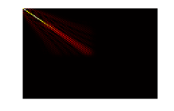
Figure 1: $\|A^{\mathbbm{J}}_{i,j}\|$ on the left and $\|A^{DFT}_{i,j}\|$ on the right in both case $1\leq i,j\leq 400$

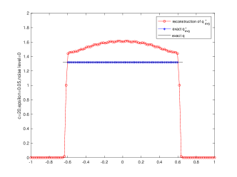
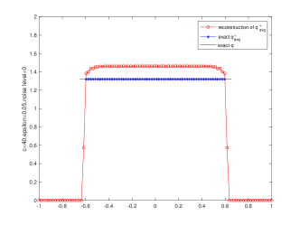
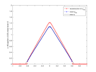
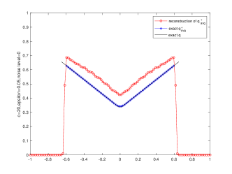
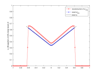
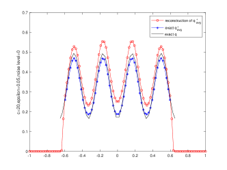
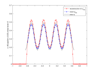
Figure 2: Plot of $I(z)$, $q_{avg}$, and $q$ for four different types of parameters with noiseless data and $\epsilon=5\times 10^{-2}$. Left column: $\dim(\mathbb{J})=37$. Right column: $\dim(\mathbb{J})=54$. Row $j$ corresponds to type $j$, j=1,2,3,4.

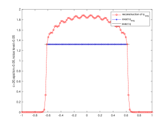
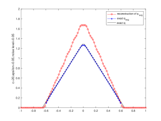
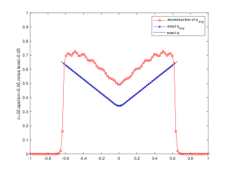
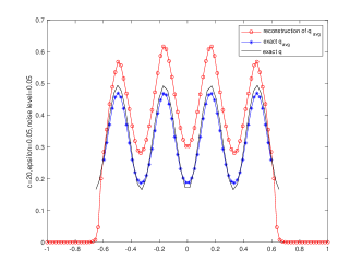
Figure 3: Plot of $I(z)$, $q_{avg}$, and $q$ for four different types of parameters with noisy level $5\%$. $\epsilon=5\times 10^{-2}$ and $c=20$.

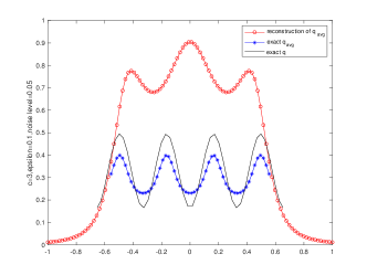
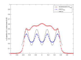
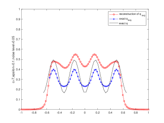
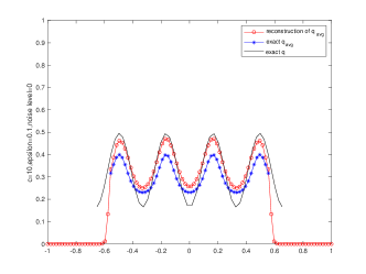
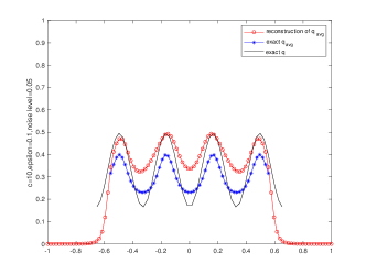
Figure 4: Plot of $I(z)$, $q_{avg}$, and $q$ for noiseless data (left column) and noisy data with noise level $\delta=5\%$ (right column). $\epsilon=1\times 10^{-1}$. From top to bottom $c=3,5,7,10$.

In the following we give details of the implementation of the prolate-Galerkin formulation of the linear sampling. The PSWFs are computed as detailed in Section 6.3 where we use the Matlab code developed in [8]. The prolate eigenvalues are then computed using the formulas (42) – (43) by adding a simple Matlab script to the existing code of [8]. The exact data are calculated analytically by hand using the four different $q$ given by (46)–(49). Given a noisy operator $\mathcal{N}^{\delta}$, we obtain a noisy data matrix $A^{\mathbbm{J},\delta}$ according to (45) so that

$$A^{\mathbbm{J},\delta}_{j\ell}=\langle\mathcal{N}^{\delta}\psi_{j}(\cdot,;c),\psi_{\ell}(\cdot,;c)\rangle,\quad j,\ell\in\mathbbm{J},$$

where the noisy data are given by adding Gaussian noise to the exact data which introduce $\delta$ noise level such that $\|A^{\mathbbm{J},\delta}-A^{\mathbbm{J}}\|_{2}=\delta$. We integrate the product of the data and the PSWFs using a Legendre-Gauss-Lobatto (LGL) quadrature rule. The right hand side is given by (45) and (33) where

$$\phi^{\mathbbm{J}}_{z\ell}=\lambda_{\ell}(c)\langle E_{z},\psi_{\ell}(\cdot,;c)\rangle_{B(z,\epsilon)},\quad\ell\in\mathbbm{J},$$

here we approximate the integral over $R(z,\epsilon)$ with $R(z,\epsilon)=B(z,\epsilon)=(z-\epsilon,z+\epsilon)$ using again the Legendre-Gauss-Lobatto (LGL) quadrature rule in this interval $(z-\epsilon,z+\epsilon)$. Having a regularized solution $\{g^{{\mathbbm{J}},\delta}_{z,\alpha,j}\}_{j\in{\mathbbm{J}}}$ computed from the noisy linear system (as is similar to the noiseless case (44))

$$\sum_{j\in\mathbbm{J}}A^{\mathbbm{J},\delta}_{j\ell}g^{\mathbbm{J},\delta}_{z,\alpha,j}\sim\phi^{\mathbbm{J}}_{z\ell},\quad\ell\in\mathbbm{J},$$

we then proceed by

$$\mathcal{S}g^{{\mathbbm{J}},\delta}_{z,\alpha}=\sum_{j\in\mathbbm{J}}\overline{\lambda_{j}(c)}g^{{\mathbbm{J}},\delta}_{z,\alpha,j}\psi_{j}(\cdot;c)\mbox{ so that }\langle\mathcal{S}g^{{\mathbbm{J}},\delta}_{z,\alpha},1_{B(z,\epsilon)}\rangle=\sum_{j\in\mathbbm{J}}\overline{\lambda_{j}(c)}g^{{\mathbbm{J}},\delta}_{z,\alpha,j}\langle\psi_{j}(\cdot;c),1_{B(z,\epsilon)}\rangle_{{}_{B(z,\epsilon)}}$$

and approximate each integral $\langle\psi_{j}(\cdot;c),1_{B(z,\epsilon)}\rangle_{{}_{B(z,\epsilon)}}$ over $(z-\epsilon,z+\epsilon)$ using again the Legendre-Gauss-Lobatto (LGL) quadrature rule. We further set the indicator function by

$$I(z):=\big{(}\langle\mathcal{S}g^{{\mathbbm{J}},\delta}_{z,\alpha},1_{B(z,\epsilon)}\rangle\big{)}^{-1},$$

which is an harmonic mean, as expected the numerical examples confirm the well known fact that harmonic mean are larger than the classical mean. We chose in this paper the spectral cut off regularization where we chose $\mathbbm{J}$ such that all the corresponding prolate eigenvalues (with indexes in $\mathbbm{J}$) are larger that the noise level $\delta$.

First we illustrate in figure 1 the fact that PSWFs compressed the data operator where we compare the operator expressed in PSWFs basis which is the matrix $A^{\mathbbm{J}}$ with the operator $\mathcal{N}$ discretize on a cartesian grid and computed using Discrete (fast) Fourrier Transform which is the matrix $A^{DFT}$.

Motivated by the particular example in Section 6.1, it is likely that we need a large index set ${\mathbb{J}}$ to achieve a sufficiently good approximation to the unknown. This first motivates us to perform a set of numerical examples with noiseless data where a large index set ${\mathbb{J}}$ can be available (the index set ${\mathbb{J}}$ cannot be too large since this means that we have to compute many prolate eigenvalues which is computationally challenging due to the super fast exponential decay of the prolate eigenvalues; see also the particular example studied in Section 6.1).

In figure 2, we plot the indicator function $I(z)=[\langle\mathcal{S}g^{{\mathbbm{J}},\delta}_{z,\alpha},1_{B(z,\epsilon)}\rangle]^{-1}$ with noiseless data, $\epsilon=0.05$, and two different $c$. Here $c=20$ (left column) allows us to have an index set ${\mathbbm{J}}$ of dimension $37$ and $c=40$ (right column) allows us to have an index set ${\mathbbm{J}}$ of dimension $54$. We approximate all integrals using a Legendre-Gauss-Lobatto (LGL) quadrature rule with $100$ quadrature nodes. The Matlab command “ro-” line represents the indicator function $I(z)$, which is an approximation (according to Theorem 4) to

$$q_{avg}(z):=\big{(}\langle 1/q,E_{z}\rangle_{L^{2}(B(z,\epsilon))}\big{)}^{-1}.$$

It is seen that $q_{avg}$ is an approximation of $q$, the Matlab command “b*-” line represents $q_{avg}(z)$ (plotted only in $(-r+\epsilon,r-\epsilon)$) and the Matlab command “k-” line represents the exact ${q}$ (plotted only in $(-r,r)$). The four types of parameters are given by setting $r=0.66$ (which is roughly $2/3$) in (46)–(49) and we set $m=4$ to have $4$ oscillations in the case of oscillatory $q$. It is observed that the larger the index set ${\mathbbm{J}}$, the better the convergence.

To further demonstrate its viability, we report the results in Figure 3 by changing the noise level to $5\%$ for the case when $c=20$. The robustness of LSM with respect to noises is observed.

The next set of examples in Figure 4 is devoted to testing the performance with respect to different $c$ for both noiseless and noisy data. We observe that larger $\epsilon$ is expected to give better convergence for parameter identification, thereby in order to observe a possible convergence for noisy data, we set $\epsilon=1\times 10^{-1}$ in this set of examples. In the case of noisy data we set noisy level $\delta=5\times 10^{-2}$. In these examples, we apply the LGL quadrature rule with $100$ quadrature nodes and we report that all the results hold similarly with $40$ quadrature nodes. In the case of noiseless data, we observe similar performance with respect to different $c$; in the case of noisy data, we observe that the performance becomes better as $c$ becomes larger.

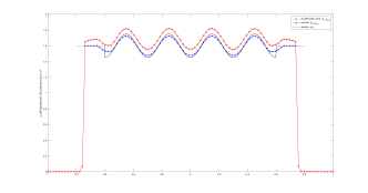
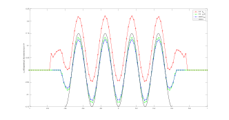
Figure 5: Plot of $I(z)$, $q+q_{inf}$ on the left and $I(z)-q_{inf}(z)$, $I(z)-I_{inf}(z)$, $q$ on the right and noiseless data with $\epsilon=5\times 10^{-1}$ and $c=40$.

To illustrate the case of sign changing parameter we report the results in Figure 5. First we show the reconstruction of $q+q_{inf}1_{D}$ for $D$ of radius 0.8 where $\Omega$ is of radius 0.6 which are similar to the one from the previous examples. Then we show the comparison between $I(z)-q_{inf}(z)$ and $I(z)-I_{inf}(z)$ and as expected by remark 6 the superiority of the second reconstruction similarly to our inspiration from [5].

To conclude this numerical section we would like to report the numerical results for disjoint supports. Figure 6 shows the results for the case of a constant $q$ with 2 connected component; the distance between the two connected components is from the set $\{1.16,0.08,0.06,0.04,0.02,0.01\}$. This case is covered by the theory but the results are very promising and theoretical analysis of the resolution limit of our method is an interesting subject for future work.

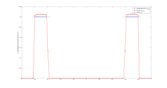
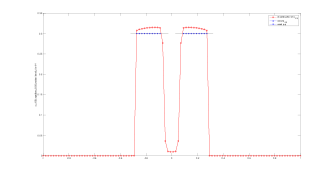
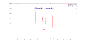
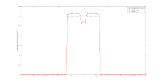
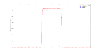
Figure 6: Plot of $I(z)$, $q_{avg}$, and $q$ for noiseless data and components getting closer and closer. $\epsilon=5\times 10^{-2}$ and $c=100$.

References

References

• [1] T Arens. Why linear sampling works, Inverse Problems 20, 163–173, 2004.
• [2] T Arens and A Lechleiter. The linear sampling method revisited, Jour. Integral Equations and Applications 21, 179–202, 2009.
• [3] T Arens and A Lechleiter. Indicator functions for shape reconstruction related to the linear sampling method, SIAM J. Imaging Sci. 8, no. 1, 513–535, 2015.
• [4] L Audibert. The Generalized Linear Sampling and factorization methods only depends on the sign of contrast on the boundary Inverse Probl. Imaging 11, no. 6, pp.  1107–1119, 2017.
• [5] L Audibert, A Girard and H  Haddar. Identifying defects in an unknown background using differential measurements Inverse Probl. Imaging 9, no. 3, pp.  625–643, 2015.
• [6] L Audibert and H Haddar. A generalized formulation of the linear sampling method with exact characterization of targets in terms of far field measurements, Inverse Problems 30, 035011, 2015.
• [7] L Bourgeois and E Lunéville. The linear sampling method in a waveguide: a modal formulation. Inverse problems 24(1), 015018, 2008.
• [8] J  Boyd. Algorithm 840: computation of grid points, quadrature weights and derivatives for spectral element methods using prolate spheroidal wave functions—prolate elements, ACM Trans. Math. Software 31, no. 1, 149–165, 2005.
• [9] F Cakoni and D Colton. Qualitative Approach to Inverse Scattering Theory, Springer, 2016.
• [10] F Cakoni, D Colton and H Haddar. Inverse Scattering Theory and Transmission Eigenvalues, CBMS-NSF, SIAM Publications 98, 2nd Edition, 2023.
• [11] D Colton and A Kirsch. A simple method for solving inverse scattering problems in the resonance region, Inverse Problems 12, pp. 383–393, 1996.
• [12] D Colton and R Kress. Inverse Acoustic and Electromagnetic Scattering Theory, Springer Nature, New York, 2019.
• [13] R Griesmaier and C Schmiedecke. A factorization method for multi-frequency inverse source problems with sparse far field measurements, SIAM J. Imag. Sci. 10, pp. 2119–2139, 2017.
• [14] M Isaev and R Novikov. Reconstruction from the Fourier transform on the ball via prolate spheroidal wave functions, Journal de Mathématiques Pures et Appliquées 163, pp.318–333, 2022.
• [15] C Kirisits, M Quellmalz, M Ritsch-Marte,O Scherzer, E Setterqvist, G Steidl. Fourier reconstruction for diffraction tomography of an object rotated into arbitrary orientations, Inverse Problems 11, 115002, 2021.
• [16] A Kirsch. Characterization of the shape of a scattering obstacle using the spectral data of the far-field operator, Inverse Problems 14, pp. 1489–1512, 1998.
• [17] A Kirsch. Remarks on the Born approximation and the Factorization Method, Applicable Analysis 96, no. 1, pp. 70–84, 2021.
• [18] A Kirsch. An Introduction to the Mathematical Theory of Inverse Problems, Springer Nature, Switzerland AG, 2021.
• [19] A Kirsch and N Grinberg. The Factorization Method for Inverse Problems, Oxford University Press, Oxford, 2008.
• [20] S Meng. A sampling type method in an electromagnetic waveguide. Inverse Probl. Imaging 15(4), 745–762, 2021.
• [21] S Meng. Single mode multi-frequency factorization method for the inverse source problem in acoustic waveguides, SIAM J. Appl. Math. 83 (2), 394–417, 2023.
• [22] S Meng. Data-driven basis for reconstructing the contrast in inverse scattering: Picard criterion, regularity, regularization, and stability, SIAM J. Appl. Math. 83 (5), 2003–2026, 2023.
• [23] S Moskow and J Schotland. Convergence and stability of the inverse Born series for diffuse waves, Inverse Problems 24, 065004, 2008.
• [24] F Natterer. The Mathematics of Computerized Tomography, SIAM, 2001.
• [25] A Quarteroni, R Sacco and F Saleri. Numerical Mathematics, Springer, 2000.
• [26] M Quellmalz, P Elbau, O Scherze and G Steidl. Motion Detection in Diffraction Tomography by Common Circle Methods, arXiv preprint, arXiv:2209/08086.
• [27] D Slepian and H  Pollak. Prolateate Spheroidal Wave Functions, Fourier Analysis and Uncertainty -I, Bell System Tech. J. 40, pp. 43–64, 1961.
• [28] D Simons, and D Wang. Spatiospectral concentration in the Cartesian plane, GEM - International Journal on Geomathematics 2, pp 1–36, 2011.
• [29] D Slepian. Prolateate Spheroidal Wave Functions, Fourier Analysis and Uncertainty -IV: Extensions to Many Dimensions; Generalized Prolate Spheroidal Functions, Bell System Tech. J. 43, pp. 3009–3057, 1964.
• [30] D Slepian. Prolate spheroidal wave functions, Fourier analysis, and uncertainty V: The discrete case, Bell System Tech. J. 57, pp.1371–1430, 1978.
• [31] L Wang. Analysis of spectral approximations using prolate spheroidal wave functions, Math. Comp. 79(270):807–827, 2010.
• [32] J Zhang, H Li, L-L Wang and Z Zhang. Ball prolate spheroidal wave functions in arbitrary dimensions, Appl. Comput. Harmon. Anal. 48, no. 2, pp.  539–569, 2020.