Generalized disorder averages and current fluctuations in run and tumble particles

Abstract

We present exact results for the fluctuations in the number of particles crossing the origin up to time $t$ in a collection of non-interacting run and tumble particles in one dimension. In contrast to passive systems, such active particles are endowed with two inherent degrees of freedom: positions and velocities, which can be used to construct density and magnetization fields. We introduce generalized disorder averages associated with both these fields and perform annealed and quenched averages over various initial conditions. We show that the variance $\sigma^{2}$ of the current in annealed versus quenched magnetization situations exhibits a surprising difference at short times: $\sigma^{2}\sim t$ versus $\sigma^{2}\sim t^{2}$ respectively, with a $\sqrt{t}$ behavior emerging at large times. Our analytical results demonstrate that in the strictly quenched scenario, where both the density and magnetization fields are initially frozen, the fluctuations in the current are strongly suppressed. Importantly, these anomalous fluctuations cannot be obtained solely by freezing the density field.

Introduction: One-dimensional diffusive systems are known to exhibit a surprising characteristic in which they retain memory of their initial conditions indefinitely, i.e. even at late times the behavior of the system is influenced by how it was set up Le Doussal and Machta (1989); Van Beijeren (1991); Derrida and Gerschenfeld (2009a); Ferrari (2010); Lizana et al. (2010); Leibovich and Barkai (2013); Krapivsky and Meerson (2012); Krapivsky et al. (2014); Banerjee et al. (2022). In analogy with disordered systems Mézard et al. (1987); Binder and Young (1986); Nishimori (2001); Bouchaud and Georges (1990), there are two main types of initial conditions that are commonly studied. In the first, referred to as “annealed”, averages are performed over all possible trajectories allowing for equilibrium fluctuations in the initial positions of particles while in the second, referred to as “quenched”, the initial positions of particles are held fixed Derrida and Gerschenfeld (2009a); Krapivsky and Meerson (2012); Cividini and Kundu (2017); Banerjee et al. (2022); Krapivsky et al. (2014). A quantity of central interest that is used to understand the effect of such initial conditions in one-dimensional stochastic systems is the integrated current i.e. the flux $Q$ of particles, across the origin up to time $t$. There have been several studies on the statistics of $Q$ for different systems such as a collection of non-interacting random walkers, symmetric simple exclusion process (SSEP), amongst others Derrida (2007); Derrida and Gerschenfeld (2009b, a); Krapivsky and Meerson (2012); Mallick et al. (2022); Dandekar et al. (2023); Dean et al. (2023). The mean of $Q$ which is a self-averaging quantity exhibits the same behavior for different initial conditions Krapivsky and Meerson (2012). However, the fluctuations of $Q$ strongly depend on how the system is set up at $t=0$, with annealed initial conditions displaying larger fluctuations Banerjee et al. (2022). Interestingly, the variance of $Q$ for these systems exhibits a $\sqrt{t}$ behavior at all times, with the coefficient determined by the type of initial conditions being employed. While there has been extensive research on current fluctuations in such passive systems Derrida (2007); Derrida and Gerschenfeld (2009b, a); Krapivsky and Meerson (2012); Mallick et al. (2022); Derrida et al. (2004); Bodineau and Derrida (2006, 2007); Dandekar et al. (2023); Krapivsky et al. (2015); Dandekar and Mallick (2022); Dean et al. (2023), there have been relatively few studies of fluctuations in active systems Banerjee et al. (2020); Agranov et al. (2023); Jose et al. (2023); Di Bello et al. (2023).

Active systems consist of particles that perform directed motion by consuming energy at the microscopic level, and represent an important paradigm in non-equilibrium physics Vicsek et al. (1995); Czirók et al. (1999); Tailleur and Cates (2008); Cavagna et al. (2010); Cates (2012); Ramaswamy (2010). Several microscopic models of active motion have been studied in detail in the literature Evans and Majumdar (2018); Malakar et al. (2018); Mori et al. (2020a, b); Angelani et al. (2014); Martens et al. (2012); Jose et al. (2022); Jose (2022); Lindner and Nicola (2008); Basu et al. (2018); Kumar et al. (2020); Romanczuk and Erdmann (2010); Romanczuk et al. (2012); Das et al. (2018); Caprini and Marconi (2019); Sevilla et al. (2019); Le Doussal et al. (2019). A theoretically appealing class of active motion is the run and tumble particle (RTP) motion Evans and Majumdar (2018); Malakar et al. (2018); Mori et al. (2020a, b); Angelani et al. (2014); Martens et al. (2012); Jose et al. (2022); Jose (2022), in which an organism moves in a straight line (run) for a certain period of time, and then randomly changes direction (tumbles), before resuming another run. Recently Banerjee et al. (2020), it was shown that for non-interacting RTPs in one dimension, the variance of $Q$ displays a linear $t$ behavior at short times and a $\sqrt{t}$ behavior at large times. Similar to the case of passive particles, the coefficients governing these fluctuations differ for quenched and annealed initial conditions associated with the positions of the particles. However, in contrast to passive particles, whose motion is governed solely by random thermal fluctuations, the self-propulsion of active particles endows them with an additional degree of freedom: their internal bias direction. This opens up an intriguing possibility of constructing annealed and quenched disorder averages associated with both the positions and velocities of active particles.

In this Letter, we introduce generalized disorder averages for active particle systems which can lead to surprising differences in transport properties including the distribution of the particle flux $Q$ across the origin. Focusing on the case of non-interacting run and tumble particles in one dimension, we derive exact results for the fluctuations in $Q$ for each of the four types of disorder averages (quenched or annealed initial conditions for the positions and velocities respectively). Our analytic results demonstrate that for quenched initial conditions associated with both the positions and velocities of the particles, the current fluctuations are anomalously suppressed at short times. This suppression is characterized by a $t^{2}$ behavior in the variance of $Q$, as opposed to a $t$ behavior displayed in the other cases. This peculiar difference in growth exponents for different initial conditions does not seem to have an analogue in passive systems, where the initial conditions only give rise to different prefactors. Crucially, this anomalous suppression of fluctuations cannot be achieved by quenching the initial positions alone, highlighting the importance of considering both the positions and velocities of active particles in defining disorder averages.

Microscopic model: We consider $N$ independent run and tumble particles evolving according to the Langevin equation

$$\frac{\partial x_{i}(t)}{\partial t}=vm_{i}(t),~{}v>0,~{}1<i<N,$$ (1)

in one dimension. Here, $m_{i}(t)$ is a stochastic variable that can switch values between $+1$ and $-1$ at a Poissonian rate $\gamma$. If $m_{i}(t)=+1$, the $i^{\text{th}}$ particle is in $+$ state at time $t$ and performs a biased motion towards the right. If $m_{i}(t)=-1$, the $i^{\text{th}}$ particle is in $-$ state at time $t$ and performs a biased motion towards the left.

Figure 1: Schematic diagram depicting the trajectories of non-interacting active particles in one dimension. The system is initiated using a step density profile, with all particles uniformly distributed to the left of the origin at time $t=0$. The initial positions and bias states of the particles are denoted by $\{x_{i}\}$ and $\{m_{i}\}$ respectively.

We consider a finite one-dimensional box bounded between $[-L,~{}0]$ with $N$ particles and then eventually take the infinite system size limit. The positions of the particles $x_{i}(t)$ can be used to construct a density field $\rho(x,t)=L^{-1}\sum_{i=1}^{N}\delta(x-x_{i}(t))$. Since the velocities resemble internal spin states, we construct a corresponding magnetization field $m(x,t)=L^{-1}\sum_{i=1}^{N}m_{i}(t)\delta(x-x_{i}(t))$ associated with the internal bias of the particles. For brevity, we denote the positions and bias states of particles at time $t=0$ by $\{x_{i}\}$ and $\{m_{i}\}$ respectively. Each position $x_{i}$ is drawn from a uniform distribution between $-L$ and $0$ with $0>x_{1}>x_{2}>x_{3}\ldots$. The initial bias state $m_{i}$ can be $+$ or $-$ with probability $1/2$. This corresponds to a step initial density profile, $\rho(x,0)=\rho\theta(-x)$, where $\rho=N/L$ and a zero initial magnetization, $m(x,0)=0$.

The number of particles $Q$, that cross the origin up to time $t$, can be computed as follows: when a particle crosses the origin from left to right, it contributes $+1$ to $Q$, and when a particle crosses from right to left, it contributes $-1$. Therefore, the integrated current up to time $t$ is exactly equal to the number of particles on the positive-half infinite line ($x>0$) at time $t$. The dynamics of a system of non-interacting RTPs is depicted in Fig. 1.

Summary of the main results: We compute the statistics of $Q$ for various initial conditions. We first consider an annealed density and annealed magnetization setting. This allows for equilibrium fluctuations in the positions and velocities of particles at time $t=0$. This is the specific case studied in Banerjee et al. (2020). As we show, another equivalent scenario is the annealed density and quenched magnetization setting where the positions are allowed to fluctuate, but the velocities are fixed at time $t=0$. The explicit expression for the variance of $Q$ for both these cases are the same and are given as Banerjee et al. (2020)

$$\sigma_{a,a}^{2}=\sigma_{a,q}^{2}=\frac{\rho v}{2}te^{-t\gamma}(\boldsymbol{I}_{0}(t\gamma)+\boldsymbol{I}_{1}(t\gamma)).$$ (2)

Here, $\boldsymbol{I}_{0}$ and $\boldsymbol{I}_{1}$ are modified Bessel functions. The first and second subscripts denote the type of averaging done for the density and the magnetization fields respectively ($``a"$ for annealed and $``q"$ for quenched). The above expression has the limiting behaviors

$$\sigma_{a,a}^{2}=\sigma_{a,q}^{2}\approx\begin{cases}\frac{\rho v}{2}t,&\text{for }t\rightarrow 0,\\ \rho\sqrt{\frac{{D_{\text{eff}}}~{}{t}}{{\pi}}},&\text{for }t\rightarrow\infty,\end{cases}$$ (3)

where $D_{\text{eff}}=v^{2}/(2\gamma)$ is the effective diffusion constant for RTP motion in one dimension. The mean of $Q$, which is a self-averaging quantity assumes the same form for all initial conditions, and is also given by Eq. (2).

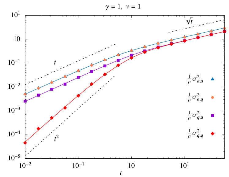
Figure 2: Variance of the integrated current plotted as a function of time for different initial conditions. The solid curves correspond to the theoretical results provided in Eqs. (2), (4) and (6) and the points are from numerical simulations of the microscopic model. For quenched density and quenched magnetization initial conditions, the fluctuations surprisingly exhibit a $t^{2}$ behavior at short times.

In the quenched density and quenched magnetization setting, the initial positions and velocities of the particles are held fixed. The variance $\sigma_{q,q}^{2}$ for this case can be computed as

$$\sigma_{q,q}^{2} = \frac{\rho v}{4}te^{-2\gamma t}\Big{[}(2+\pi\boldsymbol{L}_{0}(2t\gamma))\boldsymbol{I}_{1}(2t\gamma)$$ (4)

$$- \pi\boldsymbol{L}_{1}(2t\gamma)\boldsymbol{I}_{0}(2t\gamma)\Big{]},$$

where $\boldsymbol{L}_{0}$ and $\boldsymbol{L}_{1}$ are modified Struve functions. The above expression has the limiting behaviors

$$\sigma_{q,q}^{2}\approx\begin{cases}\frac{\rho v\gamma}{2}t^{2},&\text{for }t\rightarrow 0,\\ \rho\sqrt{\frac{{D_{\text{eff}}}~{}{t}}{2{\pi}}},&\text{for }t\rightarrow\infty.\end{cases}$$ (5)

We notice that for the case where both the fields are quenched initially, the fluctuations surprisingly exhibit a $t^{2}$ behavior at short times.

The final case we study is the quenched density and annealed magnetization setting where the initial positions of the particles are fixed, but the velocities are allowed to fluctuate. This non-trivial case is usually difficult to analyze, nevertheless we have exactly computed the variance $\sigma_{q,a}^{2}$ which has the explicit form

$$\sigma_{q,a}^{2} = \frac{\rho v}{8}te^{-2\gamma t}\Big{[}(4+\pi\boldsymbol{L}_{0}(2t\gamma))\boldsymbol{I}_{1}(2t\gamma)$$ (6)

$$+ (2-\pi\boldsymbol{L}_{1}(2t\gamma))\boldsymbol{I}_{0}(2t\gamma)\Big{]},$$

with the limiting behaviors

$$\sigma_{q,a}^{2}\approx\begin{cases}\frac{\rho v}{4}t,&\text{for }t\rightarrow 0,\\ \rho\sqrt{\frac{{D_{\text{eff}}}~{}{t}}{2{\pi}}},&\text{for }t\rightarrow\infty.\end{cases}$$ (7)

These asymptotic behaviors were also computed numerically in Ref. Banerjee et al. (2020). Our analytic expressions obtained in Eqs. (2), (4) and (6) are compared with direct numerical simulations in Fig. 2. We find excellent agreement between our theoretical predictions and the Monte Carlo simulation results.

In the calculations that follow, the angular bracket $\langle\cdots\rangle_{\{x_{i}\},\{m_{i}\}}$ denotes an average over the history (equivalent to a partition function), but with fixed initial positions $\{x_{i}\}$ and bias states $\{m_{i}\}$. We use $\overline{\cdots}$ to denote an average over initial positions and $\overbrace{\cdots}$ to denote an average over initial bias states. We consider different initial conditions separately.

Annealed density and annealed magnetization: We first consider annealed density and annealed magnetization initial conditions. The flux distribution for this case is denoted as $P_{a,a}(Q,t)$. The moment-generating function for this distribution is given as

$$\sum_{Q=0}^{\infty}e^{-pQ}P_{a,a}(Q,t)=\overbrace{\overline{\langle e^{-pQ}\rangle_{\{x_{i}\},\{m_{i}\}}}}.$$ (8)

The quantity $\langle e^{-pQ}\rangle_{\{x_{i}\},\{m_{i}\}}$ appears in the expressions for the moment and cumulant generating functions of the flux distributions for different initial conditions. This quantity has been computed in Banerjee et al. (2020) for the case where one field (density) is considered. We extend the definition to incorporate the magnetization field, which yields

$$\langle e^{-pQ}\rangle_{\{x_{i}\},\{m_{i}\}}=\prod_{i=1}^{N}\left[1-(1-e^{-p})U^{m_{i}}(-x_{i},t)\right],$$ (9)

where

$$U^{m_{i}}(-x_{i},t)=\int_{0}^{\infty}dx~{}G^{m_{i}}(x,x_{i},t),$$ (10)

is the integral of the single-particle Green’s function $G^{m_{i}}(x,x_{i},t)$. The Green’s function $G^{m_{i}}(x,x_{i},t)$ gives the probability density of finding a particle at the location $x$ at time $t$, starting from the location $x_{i}$ in the bias state $m_{i}$ at time $t=0$, and have not been derived previously. We present a detailed derivation of the Green’s functions $G^{m_{i}}(x,x_{i},t)$ for different initial bias states in the Supplemental Material SI .

To perform an average over initial positions, we consider the position of each particle to be distributed uniformly in the box $[-L,0]$, and eventually take a $L\rightarrow\infty,~{}N\rightarrow\infty$ limit with $N/L\rightarrow\rho$ fixed. After performing an average over the initial positions in Eq. (9), we obtain

$$\overline{\langle e^{-pQ}\rangle_{\{x_{i}\},\{m_{i}\}}} = \prod_{i=1}^{N}\left[1-(1-e^{-p})\overline{U^{m_{i}}(-x_{i},t)}\right]$$

$$= \left[1-\frac{1}{L}(1-e^{-p})\int_{0}^{L}dz~{}U^{m_{z}}(z,t)\right]^{N}.$$

Here, $m_{z}$ denotes the bias state of the particle located at $x_{i}=-z$ at time $t=0$. Next performing an average over initial bias states in the above equation, we obtain

$$\overbrace{\overline{\langle e^{-pQ}\rangle_{\{x_{i}\},\{m_{i}\}}}} = \left[1-\frac{1}{L}(1-e^{-p})\int_{0}^{L}dz~{}U^{0}(z,t)\right]^{N},$$

where

$$U^{0}(z,t)=\left(U^{+}(z,t)+U^{-}(z,t)\right)/2.$$ (13)

Taking the limit $N\to\infty$, $L\to\infty$ keeping $\rho=N/L$ fixed yields

$$\sum_{Q=0}^{\infty}e^{-pQ}P_{a,a}(Q,t) = \overbrace{\overline{\langle e^{-pQ}\rangle_{\{x_{i}\},\{m_{i}\}}}}$$ (14)

$$\rightarrow \exp\left[-\mu(t)~{}(1-e^{-p})\right],$$

where

$$\mu(t)=\rho\int_{0}^{\infty}dz~{}U^{0}(z,t).$$ (15)

The above expression is exactly the moment-generating function for a Poisson distribution. Therefore, $P_{a,a}(Q=N,t)$ is always a Poisson distribution Banerjee et al. (2020) with

$$P_{a,a}(Q=N,t)=e^{-\mu(t)}\frac{\mu(t)^{N}}{N!},~{}N~{}=0,1,2,\cdots~{},$$ (16)

and the mean and the variance are both given by $\mu(t)$. We thus obtain

$$\sigma_{a,a}^{2}(t)=\mu(t).$$ (17)

The explicit expression for $\sigma_{a,a}^{2}$ can be directly computed using Eq. (15) and we obtain the announced result in Eq. (2). The derivation of this expression is provided in the Supplemental Material SI .

Annealed density and quenched magnetization: We next consider annealed density and quenched magnetization initial conditions. The flux distribution for this case is denoted as $P_{a,q}(Q,t)$. The moment-generating function for this flux distribution is given as

$$\sum_{Q=0}^{\infty}e^{-pQ}P_{a,q}(Q,t)=\exp\left[\overbrace{\ln\overline{\langle e^{-pQ}\rangle_{\{x_{i}\},\{m_{i}\}}}}\right].$$ (18)

Using Eq. (LABEL:history_pos_av), we directly compute the cumulant generating function as

$$\overbrace{\ln\overline{\langle e^{-pQ}\rangle_{\{x_{i}\},\{m_{i}\}}}}=$$

$$\overbrace{\ln\left[1-\frac{1}{L}(1-e^{-p})\int_{0}^{L}dz~{}U^{m_{z}}(z,t)\right]^{N}}\rightarrow-\mu(t)(1-e^{-p}),$$

where $\mu(t)$ is defined in Eq. (15). In the large system size limit ($L\rightarrow\infty,~{}N\rightarrow\infty,~{}N/L\rightarrow\rho$), the distribution $P_{a,q}(Q,t)$ is equivalent to the distribution $P_{a,a}(Q,t)$. This is because keeping the velocities fixed or allowing them to fluctuate does not make a difference in the annealed density setting as the initial positions of particles are randomized. Thus we obtain the identity in Eq. (2).

Quenched density and quenched magnetization: The third case we study is the quenched density and quenched magnetization initial conditions. The flux distribution for this case is denoted as $P_{q,q}(Q,t)$. The moment-generating function is given as

$$\sum_{Q=0}^{\infty}e^{-pQ}P_{q,q}(Q,t)=\exp\left[\overbrace{\overline{\ln\langle e^{-pQ}\rangle_{\{x_{i}\},\{m_{i}\}}}}\right].$$ (20)

Taking the logarithm on both sides of Eq. (9) yields

$${\ln}\left[\langle e^{-pQ}\rangle_{\{x_{i}\},\{m_{i}\}}\right]=\sum_{i=1}^{N}{\ln}\left[1-(1-e^{-p})U^{m_{i}}(-x_{i},t)\right].$$ (21)

After performing an average over the initial positions and the velocities, we obtain the expression for the cumulant generating function as

$$\overbrace{\overline{\ln\left[\langle e^{-pQ}\rangle_{\{x_{i}\},\{m_{i}\}}\right]}} = \frac{\rho}{2}\int_{0}^{\infty}dz\ln\left[1-(1-e^{-p})U^{+}(z,t)\right]$$

$$+ \frac{\rho}{2}\int_{0}^{\infty}dz\ln\left[1-(1-e^{-p})U^{-}(z,t)\right].$$

The cumulants can be extracted by collecting terms that appear in the same powers of $p$. This yields the expressions for the mean and variance of $Q$ as

$$\langle Q\rangle_{q,q} = \mu(t),$$

$$\sigma_{q,q}^{2} = \langle Q^{2}\rangle_{q,q}-\langle Q\rangle^{2}_{q,q}$$ (23)

$$= \frac{\rho}{2}\int_{0}^{\infty}dz~{}\left[U^{+}(z,t)(1-U^{+}(z,t))\right]$$

$$+ \frac{\rho}{2}\int_{0}^{\infty}dz~{}\left[U^{-}(z,t)(1-U^{-}(z,t))\right],$$

where $\mu(t)$ is defined in Eq. (15) and the explicit expression for $\mu(t)$ is provided in Eq. (2). One can also derive the explicit expression for the variance using Eq. (23). Thus we obtain the announced result in Eq. (4). See SI for details related to the derivation of this expression.

Quenched density and annealed magnetization: Finally, we study quenched density and annealed magnetization initial conditions. The flux distribution for this case is denoted as $P_{q,a}(Q,t)$. The moment-generating function for this process is given as

$$\sum_{Q=0}^{\infty}e^{-pQ}P_{q,a}(Q,t)=\exp\left[\overline{\ln\overbrace{\langle e^{-pQ}\rangle_{\{x_{i}\},\{m_{i}\}}}}\right].$$ (24)

After performing an average over the initial velocities in Eq. (9), we obtain

$$\overbrace{\langle e^{-pQ}\rangle_{\{x_{i}\},\{m_{i}\}}} = \prod_{i=1}^{N}\left[1-(1-e^{-p})\overbrace{U^{m_{i}}(-x_{i},t)}\right]$$

$$= \prod_{i=1}^{N}\left[1-(1-e^{-p})U^{0}(-x_{i},t)\right],$$

where $U^{0}$ is defined in Eq. (13). Next, we compute the cumulant generating function as

$$\overline{\ln\overbrace{\langle e^{-pQ}\rangle_{\{x_{i}\},\{m_{i}\}}}}$$

$$=\frac{N}{L}\int_{-L}^{0}dx_{i}~{}{\ln}\left[1-(1-e^{-p})U^{0}(-x_{i},t)\right]$$

$$\longrightarrow\rho\int_{0}^{\infty}dz\ln\left[1-(1-e^{-p})U^{0}(z,t)\right].$$

Collecting terms that appear in the first and second powers of $p$, we obtain the expressions for the mean and variance of $Q$ as

$$\langle Q\rangle_{q,a} = \mu(t),$$

$$\sigma_{q,a}^{2} = \langle Q^{2}\rangle_{q,a}-\langle Q\rangle^{2}_{q,a}$$ (26)

$$= \rho\int_{0}^{\infty}dz~{}\left[U^{0}(z,t)\left(1-U^{0}(z,t)\right)\right],$$

where $\mu(t)$ is defined in Eq. (15) and the explicit expression for $\mu(t)$ is provided in Eq. (2). The explicit expression for the variance can also be computed using the single-particle Green’s functions SI and we obtain the announced result in Eq. (6).

Discussion: In this Letter, we have introduced generalized disorder averages for active systems that account for fluctuations in both the initial positions and velocities of particles. We illustrated these averages in a one-dimensional system of non-interacting RTPs, and derived exact results for the fluctuations in the integrated current across the origin up to time $t$. Surprisingly, these fluctuations display different growth exponents at short times for different initial conditions, a feature that does not seem to occur in passive systems. Specifically, we observed suppressed fluctuations for the case when both the positions and velocities are initially quenched, characterized by a $t^{2}$ growth in the variance, as opposed to a linear $t$ behavior observed in the other cases. At large times, a $\sqrt{t}$ behavior emerges, consistent with late time diffusive behavior, with the quenched and annealed density settings differing by a factor of $\sqrt{2}$ Leibovich and Barkai (2013); Banerjee et al. (2020); Derrida and Gerschenfeld (2009a); Krapivsky and Meerson (2012).

Such generalized disordered averages can also be extended to a variety of other models with multiple degrees of freedom at the particle level. While the exact results reported in this Letter are specific to non-interacting RTPs in one dimension, we expect the derived asymptotic behaviors to hold in other active systems as well. In particular, we expect other models of active motion such as active Brownian particles Lindner and Nicola (2008); Basu et al. (2018); Kumar et al. (2020); Romanczuk and Erdmann (2010); Romanczuk et al. (2012) as well as interacting active particles in the low-density limit Kourbane-Houssene et al. (2018); Agranov et al. (2021); Jose et al. (2023); Agranov et al. (2022) to display similarly suppressed fluctuations for quenched initial conditions. Additionally, we also expect the surprising differences in the growth exponents governing the current fluctuations for different initial conditions to appear in higher dimensions as well.

Several interesting directions for further research remain. It would be instructive to compute the higher-order cumulants of the current, in order to better understand the differences between quenched and annealed disorder in active systems. It would also be interesting to verify our predictions by implementing the different disorder averages within a fluctuating hydrodynamics framework or using Macroscopic Fluctuation Theory Bertini et al. (2005, 2006, 2007, 2009, 2015); Derrida et al. (2001); Bodineau and Derrida (2004); Derrida (2011), which have been shown to successfully predict fluctuations in many-particle systems Derrida and Gerschenfeld (2009a); Krapivsky and Meerson (2012); Krapivsky et al. (2015, 2014); Mallick et al. (2022); Derrida (2007); Rana and Sadhu (2023). Additionally, although we have considered the case of zero diffusion and symmetric initial conditions, our framework can also be extended to situations where the particles have a non-zero diffusion in their microscopic dynamics, and are initiated with asymmetric magnetization initial conditions. Finally, it would also be interesting to study the effect of generalized disorder averages on observables such as the magnetization current, which could lead to a better understanding of the differences between active and passive systems.

Acknowledgments: We thank R. Maharana, M. Barma, R. Dandekar, S. N. Majumdar and G. Schehr for useful discussions. The work of K. R. was partially supported by the SERB-MATRICS grant MTR/2022/000966. This project was funded by intramural funds at TIFR Hyderabad from the Department of Atomic Energy (DAE), Government of India.

Supplemental Material for
“Generalized disorder averages and current fluctuations in run and tumble particles”

In this document, we provide supplemental details related to the results presented in the main text. We provide expressions for single particle propagators for different initial conditions. We consider symmetric initial conditions where a Run and Tumble Particle (RTP) is initialized in $+$ and $-$ states with equal probability as well as asymmetric initial conditions where a RTP is initialized in either the $+$ or $-$ states. We also present detailed derivations of the exact expressions for the variance of the integrated current for quenched and annealed initial conditions involving both the density and magnetization fields.

I Single Particle Propagators

Consider an RTP starting its motion from the location $x=0$ at time $t=0$ in one dimension. Let $P_{m}(x,t)$ denote the probability density that the particle is at the location $x$ at time $t$ in the velocity state $m$, where $m=\pm$. The evolutions equations for the probability density read Malakar et al. (2018)

$$\frac{\partial P_{+}(x,t)}{\partial t} = -v\frac{\partial P_{+}(x,t)}{\partial x}-\gamma P_{+}(x,t)+\gamma P_{-}(x,t),$$

$$\frac{\partial P_{-}(x,t)}{\partial t} = +v\frac{\partial P_{-}(x,t)}{\partial x}-\gamma P_{-}(x,t)+\gamma P_{+}(x,t).$$ (27)

The total probability density to be at location $x$ at time $t$ is defined as

$$P(x,t)=P_{+}(x,t)+P_{-}(x,t).$$ (28)

Let us define the Fourier transform of the probability density $P_{m}(x,t)$ as

$$\tilde{P}_{m}(k,t)=\int_{-\infty}^{\infty}~{}dk{e}^{ikx}P_{m}(x,t),$$ (29)

and the inverse Fourier transform as

$$P_{m}(x,t)=\frac{1}{2\pi}\int_{-\infty}^{\infty}~{}dx{e}^{-ikx}\tilde{P}_{m}(k,t).$$ (30)

Taking a Fourier transform of Eq. (27) yields the matrix equation

$$\frac{\partial}{\partial t}\ket{\tilde{P}_{m}(k,t)}=\mathcal{A}(k)\ket{\tilde{P}_{m}(k,t)},$$ (31)

where the ket $\ket{\tilde{P}_{m}(k,t)}$ denotes the column vector ${\begin{pmatrix}\tilde{P}_{+}(k,t)\\ \tilde{P}_{-}(k,t)\end{pmatrix}}$, and the matrix $\mathcal{A}(k)$ is given as

$$\mathcal{A}(k)=\begin{pmatrix}-\gamma+ivk&\gamma\\ \gamma&-\gamma-ivk\end{pmatrix}.$$ (32)

We next define the Laplace transform of $P_{m}(x,t)$ as

$$\tilde{P}_{m}(x,s)=\int_{0}^{\infty}~{}dt{e}^{-st}P_{m}(x,t).$$ (33)

Taking a Laplace transform of Eq. (31) yields

$$\left[s\mathcal{I}-\mathcal{A}(k)\right]~{}\ket{\tilde{P}_{m}(k,s)}=\ket{\tilde{P}_{m}(k,t=0)},$$ (34)

where $\mathcal{I}$ is the two dimensional identity matrix.

I.1 Symmetric initial conditions

We first consider the case of a single RTP initiated symmetrically in the states, $+$ and $-$. At time $t=0$, the particle has an equal probability to be in the state $+$ or $-$. Therefore,

$$P_{+}(x,0)=P_{-}(x,0)=\frac{1}{2}\delta(x).$$ (35)

In Fourier space, these initial conditions translate to $\ket{\tilde{P}_{m}(k,t=0)}~{}=~{}{\begin{pmatrix}1/2~{}1/2\end{pmatrix}}^{T}$. Solving Eq. (34) along with these initial conditions yields the exact expression for the Fourier-Laplace transform of the total probability density as

$$\tilde{P}(k,s)=\frac{s+2\gamma}{s(s+2\gamma)+v^{2}k^{2}},$$ (36)

where $\tilde{P}(k,s)~{}=~{}\tilde{P}_{+}(k,s)+\tilde{P}_{-}(k,s)$. We next invert the Fourier transform in the above equation to obtain

$$\tilde{P}(x,s)={\rm e}^{-|x|\lambda}\frac{\lambda}{2s},$$ (37)

where $\lambda$ is defined as

$$\lambda=\frac{\sqrt{s(s+2\gamma)}}{v}.$$ (38)

Let us define the Green’s function $G^{0}(x,x_{i},t)$ as the probability density of finding an RTP at location $x$ at time $t$, starting from the location $x_{i}$ at time $t=0$ with equal probabilities to be in $+$ or $-$ state. Here, the superscript $``0"$ denotes the symmetric case where the particle has an equal probability to in $+$ or $-$ state at time $t=0$. Since the evolution equations for an RTP are translationally invariant, Eqs. (37) and (38) directly yield

$$\tilde{G}^{0}(x,-z,s) = \frac{e^{-\frac{\left|x+z\right|\sqrt{s(s+2\gamma)}}{v}}\sqrt{s(s+2\gamma)}}{2vs},\quad z=-x_{i},$$ (39)

where $G^{0}(x,-z,s)$ is the Laplace transform of the Green’s function for an RTP initialized symmetrically in $+$ and $-$ states. It is useful to compute certain quantities related to the Green’s function for the analytical calculations presented in the main text. Let us first define

$$U^{0}(z,t)=\int_{0}^{\infty}dx~{}G^{0}(x,-z,t),\quad z\geq 0,$$ (40)

as the integral of the Green’s function $G^{0}(x,-z,t)$ over the half-infinite line. Using the expression in Eq. (39), we obtain the exact expression for $U^{0}(z,t)$ in Laplace space as

$$\tilde{U}^{0}(z,s) = \frac{\exp\left(-z\frac{\sqrt{s(s+2\gamma)}}{v}\right)}{2s}.$$ (41)

The integral of the function $\tilde{U}^{0}(z,s)$ over $z$ can be easily computed as

$$\int_{0}^{\infty}dz~{}\tilde{U}^{0}(z,s)=\frac{v}{2s^{3/2}\sqrt{(s+2\gamma)}}.$$ (42)

We next define

$$\tilde{V}^{0}(z,s)=\mathcal{L}\left[{U^{0}(z,t)}^{2}\right],$$ (43)

as the Laplace transform of the square of the function $U^{0}(z,t)$. The integral of the function $\tilde{V}^{0}(z,s)$ is another useful quantity that enters into the computations presented in the main text. It can be shown that

$$\int_{0}^{\infty}dz~{}\tilde{V}^{0}(z,s)=\frac{v}{2s^{3/2}}\left(\frac{1}{\sqrt{s+2\gamma}}-\frac{\sqrt{s+4\gamma}}{2(s+2\gamma)}\right).$$ (44)

I.2 Asymmetric initial conditions

We next compute the Green’s functions for initial conditions where the particle is initialized in either of the two states $+$ or $-$. We analyze these cases separately.

I.2.1 Particle initialized in $+$ state:

We first consider asymmetric initial conditions of the form

$$P_{+}(x,0)=\delta(x),\quad P_{-}(x,0)=0.$$ (45)

Here, the particle starts from $+$ velocity state at time $t=0$. In Fourier space, these initial conditions assume the form $\ket{\tilde{P}_{m}(k,t=0)}~{}=~{}{\begin{pmatrix}1~{}0\end{pmatrix}}^{T}$. Solving Eq. (34) along with these initial conditions yields the exact expression for the Fourier-Laplace transform of the total probability density as

$$\tilde{P}(k,s)=\frac{s+2\gamma+ivk}{s(s+2\gamma)+v^{2}k^{2}},$$ (46)

where $\tilde{P}(k,s)~{}=~{}\tilde{P}_{+}(k,s)+\tilde{P}_{-}(k,s)$. We next invert the Fourier transform in the above equation and this yields

$$\tilde{P}(x,s)==\frac{{\rm e}^{-|x|\lambda}}{2s}\left(\lambda+\text{sgn}(x)\frac{s}{v}\right),$$ (47)

where sgn denote the sign function and the expression for $\lambda$ is provided in Eq. (38).

I.2.2 Particle initialized in $-$ state

We next consider asymmetric initial conditions of the form

$$P_{-}(x,0)=\delta(x),\quad P_{+}(x,0)=0.$$ (48)

Here, the particle starts from $-$ velocity state at time $t=0$. In Fourier space, we have $\ket{\tilde{P}_{m}(k,t=0)}~{}=~{}{\begin{pmatrix}0~{}1\end{pmatrix}}^{T}$. Solving Eq. (34) along with these initial conditions yields the exact expression for the Fourier-Laplace transform of the total probability density as

$$\tilde{P}(k,s)=\frac{s+2\gamma-ivk}{s(s+2\gamma)+v^{2}k^{2}},$$ (49)

where $\tilde{P}(k,s)~{}=~{}\tilde{P}_{+}(k,s)+\tilde{P}_{-}(k,s)$. After inverting the Fourier transform in the above equation, we directly obtain

$$\tilde{P}(x,s)=\frac{{\rm e}^{-|x|\lambda}}{2s}\left(\lambda-\text{sgn}(x)\frac{s}{v}\right),$$ (50)

where sgn denote the sign function and the expression for $\lambda$ is provided in Eq. (38).

Let us define the Green’s function $G^{\pm}(x,x_{i},t)$ as the probability density of finding an RTP at location $x$ at time $t$, starting from the location $x_{i}$ at time $t=0$ in the velocity state $\pm$. Here, the superscript $``\pm"$ denotes the asymmetric case where the particle starts from the $+$ or $-$ state at time $t=0$ with probability $1$. Since the evolution equations for an RTP are translationally invariant, Eqs. (47), (50) and (38) directly yield

$$\tilde{G}^{\pm}(x,-z,s) = \frac{e^{-\frac{\left|x+z\right|\sqrt{s(s+2\gamma)}}{v}}\left(\sqrt{s(s+2\gamma)}\pm s~{}\text{sgn}(x+z)\right)}{2vs},\quad z=-x_{i}.$$ (51)

Let us define

$$U^{\pm}(z,t)=\int_{0}^{\infty}dx~{}G^{\pm}(x,-z,t),\quad z\geq 0,$$ (52)

as the integral of the Green’s function $G^{\pm}(x,-z,t)$ over the half-infinite line. Using the expression in Eq. (51), we obtain the exact expression for the Laplace transform of $U^{\pm}(z,t)$ as

$$\tilde{U}^{\pm}(z,s) = \frac{e^{-\frac{z\sqrt{s(s+2\gamma)}}{v}}}{2s}\left(1\pm\frac{s}{\sqrt{s(s+2\gamma)}}\right).$$ (53)

The integral of the function $\tilde{U}^{\pm}(z,s)$ over $z$ yields

$$\int_{0}^{\infty}dz~{}\tilde{U}^{\pm}(z,s)=\frac{v\left(\sqrt{s(s+2\gamma)}\pm s\right)}{2s^{2}(s+2\gamma)}.$$ (54)

We next define

$$\tilde{V}^{\pm}(z,s)=\mathcal{L}\left[{U^{\pm}(z,t)}^{2}\right],$$ (55)

as the Laplace transform of the square of the function $U^{\pm}(z,t)$. It can be shown that

$$\int_{0}^{\infty}dz~{}\tilde{V}^{\pm}(z,s)=\frac{v}{s(s+2\gamma)}\left(\pm\frac{1}{4}+\frac{1}{2}\sqrt{\frac{s+2\gamma}{s}}-\frac{\gamma}{\sqrt{s(s+4\gamma)}}\pm\frac{K\left(-\frac{8\gamma(s+2\gamma)}{s^{2}}\right)}{2\pi}\right).$$ (56)

We also define

$$\tilde{V}^{\text{cross}}(z,s)=\mathcal{L}\left[U^{+}(z,t)U^{-}(z,t)\right],$$ (57)

as the Laplace transform of the product of the functions $U^{+}(z,t)$ and $U^{-}(z,t)$. Using Eq. (13) in the main text and the definitions provided in Eqs. (43) and (55) we obtain

$$\tilde{V}^{\text{cross}}(z,s)=2\tilde{V}^{0}(z,s)-\frac{1}{2}\left(\tilde{V}^{+}(z,s)+\tilde{V}^{-}(z,s)\right).$$ (58)

Integrating the above equation over $z$ and substituting the expressions provided in Eqs. (44) and (56) yield

$$\int_{0}^{\infty}dz~{}\tilde{V}^{\text{cross}}(z,s)=\frac{v}{\sqrt{s}(s+2\gamma)^{3/2}}\left(\frac{1}{2}+\frac{\gamma}{s}+\frac{\gamma\sqrt{\frac{s(s+2\gamma)}{s+4\gamma}}}{s^{3/2}}-\frac{\sqrt{s(s+2\gamma)(s+4\gamma)}}{2s^{3/2}}\right).$$ (59)

II Derivation of the expressions of the variance for different initial conditions

We next turn to the computation of the exact expression for $\mu(t)=\sigma_{a,a}^{2}=\sigma_{a,q}^{2}$ defined in Eq. (15) of the main text. This is equal to the mean of $Q$ for all initial conditions and the variance for annealed density and annealed or quenched magnetization initial conditions. In Laplace space, the expression in Eq. (15) of the main text translates to

$$\tilde{\mu}(s)=\rho\int_{0}^{\infty}dz~{}\tilde{U}^{0}(z,s).$$ (60)

Substituting Eq. (42) in the above equation and inverting the Laplace transform yields the exact expression for the variance for annealed density and annealed or quenched magnetization initial conditions. This expression is provided in Eq. (2) of the main text.

To compute the variance $\sigma_{q,q}^{2}$ for quenched density and quenched magnetization initial conditions, we rewrite the expression provided in Eq. (23) of the main text in Laplace space as

$$\tilde{\sigma}_{q,q}^{2}(s)=\frac{\rho}{2}\left(\tilde{T}_{1}(s)+\tilde{T}_{2}(s)\right),$$ (61)

where

$$\tilde{T}_{1}(s)=\mathcal{L}\left[\int_{0}^{\infty}dz~{}\left[U^{+}(z,t)(1-U^{+}(z,t))\right]\right]=\int_{0}^{\infty}dz~{}\left[\tilde{U}^{+}(z,s)-\tilde{V}^{+}(z,s)\right],$$ (62)

and

$$\tilde{T}_{2}(s)=\mathcal{L}\left[\int_{0}^{\infty}dz~{}\left[U^{-}(z,t)(1-U^{-}(z,t))\right]\right]=\int_{0}^{\infty}dz~{}\left[\tilde{U}^{-}(z,s)-\tilde{V}^{-}(z,s)\right],$$ (63)

where $\tilde{V}^{+}(z,s)$ and $\tilde{V}^{-}(z,s)$ are defined in Eq. (55). Substituting the expressions provided in equations (54) and (56) in the above equations, we obtain

$$\tilde{T}_{1}(s)=\frac{v}{4s(s+2\gamma)}+\frac{v\gamma}{s(s+2\gamma)\sqrt{s(s+4\gamma)}}-\frac{vK\left(-\frac{8\gamma(s+2\gamma)}{s^{2}}\right)}{2\pi s(s+2\gamma)},$$ (64)

and

$$\tilde{T}_{2}(s)=-\frac{v}{4s(s+2\gamma)}+\frac{v\gamma}{s(s+2\gamma)\sqrt{s(s+4\gamma)}}+\frac{vK\left(-\frac{8\gamma(s+2\gamma)}{s^{2}}\right)}{2\pi s(s+2\gamma)}.$$ (65)

Combining equations (61), (64) and (65) and inverting the resultant Laplace transform yields the result provided in Eq. (4) of the main text.

We next compute the explicit expression of the variance $\sigma_{q,a}^{2}$ for quenched density and annealed magnetization initial conditions. Using the definitions provided in Eqs. (13) and (26) of the main text, we obtain the expression for the variance in Laplace space as

$$\tilde{\sigma}_{q,a}^{2}(s)=\frac{\rho}{2}\int_{0}^{\infty}dz~{}\Big{[}\tilde{U}^{+}(z,s)+\tilde{U}^{-}(z,s)-\frac{1}{2}\tilde{V}^{+}(z,s)-\frac{1}{2}\tilde{V}^{-}(z,s)-\tilde{V}^{\text{cross}}(z,s)\Big{]}.$$ (66)

Each term in the above expression can be computed explicitly. Combining results from equations (54), (56) and (59), we directly obtain the expression for the variance in Laplace space inverting which yields the result in Eq. (6) of the main text.

References

- Le Doussal and Machta (1989) P. Le Doussal and J. Machta, Physical Review B 40, 9427 (1989).
- Van Beijeren (1991) H. Van Beijeren, Journal of Statistical Physics 63, 47 (1991).
- Derrida and Gerschenfeld (2009a) B. Derrida and A. Gerschenfeld, Journal of Statistical Physics 137, 978 (2009a).
- Ferrari (2010) P. L. Ferrari, Journal of Statistical Mechanics: Theory and Experiment 2010, P10016 (2010).
- Lizana et al. (2010) L. Lizana, T. Ambjörnsson, A. Taloni, E. Barkai, and M. A. Lomholt, Physical Review E 81, 051118 (2010).
- Leibovich and Barkai (2013) N. Leibovich and E. Barkai, Physical Review E 88, 032107 (2013).
- Krapivsky and Meerson (2012) P. Krapivsky and B. Meerson, Physical Review E 86, 031106 (2012).
- Krapivsky et al. (2014) P. Krapivsky, K. Mallick, and T. Sadhu, Physical Review Letters 113, 078101 (2014).
- Banerjee et al. (2022) T. Banerjee, R. L. Jack, and M. E. Cates, Physical Review E 106, L062101 (2022).
- Mézard et al. (1987) M. Mézard, G. Parisi, and M. A. Virasoro, Spin glass theory and beyond: An Introduction to the Replica Method and Its Applications, vol. 9 (World Scientific Publishing Company, 1987).
- Binder and Young (1986) K. Binder and A. P. Young, Reviews of Modern physics 58, 801 (1986).
- Nishimori (2001) H. Nishimori, Statistical physics of spin glasses and information processing: an introduction, 111 (Clarendon Press, 2001).
- Bouchaud and Georges (1990) J.-P. Bouchaud and A. Georges, Physics reports 195, 127 (1990).
- Cividini and Kundu (2017) J. Cividini and A. Kundu, Journal of Statistical Mechanics: Theory and Experiment 2017, 083203 (2017).
- Derrida (2007) B. Derrida, Journal of Statistical Mechanics: Theory and Experiment 2007, P07023 (2007).
- Derrida and Gerschenfeld (2009b) B. Derrida and A. Gerschenfeld, Journal of Statistical Physics 136, 1 (2009b).
- Mallick et al. (2022) K. Mallick, H. Moriya, and T. Sasamoto, Physical Review Letters 129, 040601 (2022).
- Dandekar et al. (2023) R. Dandekar, P. Krapivsky, and K. Mallick, Physical Review E 107, 044129 (2023).
- Dean et al. (2023) D. S. Dean, S. N. Majumdar, and G. Schehr, arXiv preprint arXiv:2303.08961 (2023).
- Derrida et al. (2004) B. Derrida, B. Douçot, and P.-E. Roche, Journal of Statistical Physics 115, 717 (2004).
- Bodineau and Derrida (2006) T. Bodineau and B. Derrida, Journal of Statistical Physics 123, 277 (2006).
- Bodineau and Derrida (2007) T. Bodineau and B. Derrida, Comptes Rendus Physique 8, 540 (2007).
- Krapivsky et al. (2015) P. L. Krapivsky, K. Mallick, and T. Sadhu, Journal of Statistical Physics 160, 885 (2015).
- Dandekar and Mallick (2022) R. Dandekar and K. Mallick, Journal of Physics A: Mathematical and Theoretical (2022).
- Banerjee et al. (2020) T. Banerjee, S. N. Majumdar, A. Rosso, and G. Schehr, Physical Review E 101, 052101 (2020).
- Agranov et al. (2023) T. Agranov, S. Ro, Y. Kafri, and V. Lecomte, SciPost Physics 14, 045 (2023).
- Jose et al. (2023) S. Jose, R. Dandekar, and K. Ramola, arXiv preprint arXiv:2301.10680 (2023).
- Di Bello et al. (2023) C. Di Bello, A. K. Hartmann, S. N. Majumdar, F. Mori, A. Rosso, and G. Schehr, arXiv preprint arXiv:2302.06696 (2023).
- Vicsek et al. (1995) T. Vicsek, A. Czirók, E. Ben-Jacob, I. Cohen, and O. Shochet, Physical Review Letters 75, 1226 (1995).
- Czirók et al. (1999) A. Czirók, A.-L. Barabási, and T. Vicsek, Physical Review Letters 82, 209 (1999).
- Tailleur and Cates (2008) J. Tailleur and M. Cates, Physical Review Letters 100, 218103 (2008).
- Cavagna et al. (2010) A. Cavagna, A. Cimarelli, I. Giardina, G. Parisi, R. Santagati, F. Stefanini, and M. Viale, Proceedings of the National Academy of Sciences 107, 11865 (2010).
- Cates (2012) M. E. Cates, Reports on Progress in Physics 75, 042601 (2012).
- Ramaswamy (2010) S. Ramaswamy, Annual Review of Condensed Matter Physics 1, 323 (2010).
- Evans and Majumdar (2018) M. R. Evans and S. N. Majumdar, Journal of Physics A: Mathematical and Theoretical 51, 475003 (2018).
- Malakar et al. (2018) K. Malakar, V. Jemseena, A. Kundu, K. V. Kumar, S. Sabhapandit, S. N. Majumdar, S. Redner, and A. Dhar, Journal of Statistical Mechanics: Theory and Experiment 2018, 043215 (2018).
- Mori et al. (2020a) F. Mori, P. Le Doussal, S. N. Majumdar, and G. Schehr, Physical Review Letters 124, 090603 (2020a).
- Mori et al. (2020b) F. Mori, P. Le Doussal, S. N. Majumdar, and G. Schehr, Physical Review E 102, 042133 (2020b).
- Angelani et al. (2014) L. Angelani, R. Di Leonardo, and M. Paoluzzi, The European Physical Journal E 37, 1 (2014).
- Martens et al. (2012) K. Martens, L. Angelani, R. Di Leonardo, and L. Bocquet, The European Physical Journal E 35, 1 (2012).
- Jose et al. (2022) S. Jose, D. Mandal, M. Barma, and K. Ramola, Physical Review E 105, 064103 (2022).
- Jose (2022) S. Jose, Journal of Statistical Mechanics: Theory and Experiment 2022, 113208 (2022).
- Lindner and Nicola (2008) B. Lindner and E. Nicola, The European Physical Journal Special Topics 157, 43 (2008).
- Basu et al. (2018) U. Basu, S. N. Majumdar, A. Rosso, and G. Schehr, Physical Review E 98, 062121 (2018).
- Kumar et al. (2020) V. Kumar, O. Sadekar, and U. Basu, Physical Review E 102, 052129 (2020).
- Romanczuk and Erdmann (2010) P. Romanczuk and U. Erdmann, The European Physical Journal Special Topics 187, 127 (2010).
- Romanczuk et al. (2012) P. Romanczuk, M. Bär, W. Ebeling, B. Lindner, and L. Schimansky-Geier, The European Physical Journal Special Topics 202 (2012).
- Das et al. (2018) S. Das, G. Gompper, and R. G. Winkler, New Journal of Physics 20, 015001 (2018).
- Caprini and Marconi (2019) L. Caprini and U. M. B. Marconi, Soft matter 15, 2627 (2019).
- Sevilla et al. (2019) F. J. Sevilla, A. V. Arzola, and E. P. Cital, Physical Review E 99, 012145 (2019).
- Le Doussal et al. (2019) P. Le Doussal, S. N. Majumdar, and G. Schehr, Physical Review E 100, 012113 (2019).
- (52) See Supplemental Material for details.
- Kourbane-Houssene et al. (2018) M. Kourbane-Houssene, C. Erignoux, T. Bodineau, and J. Tailleur, Physical Review Letters 120, 268003 (2018).
- Agranov et al. (2021) T. Agranov, S. Ro, Y. Kafri, and V. Lecomte, Journal of Statistical Mechanics: Theory and Experiment 2021, 083208 (2021).
- Agranov et al. (2022) T. Agranov, M. E. Cates, and R. L. Jack, Journal of Statistical Mechanics: Theory and Experiment 2022, 123201 (2022).
- Bertini et al. (2005) L. Bertini, A. De Sole, D. Gabrielli, G. Jona-Lasinio, and C. Landim, Physical Review Letters 94, 030601 (2005).
- Bertini et al. (2006) L. Bertini, A. D. Sole, D. Gabrielli, G. Jona-Lasinio, and C. Landim, Journal of Statistical Physics 123, 237 (2006).
- Bertini et al. (2007) L. Bertini, A. De Sole, D. Gabrielli, G. Jona-Lasinio, and C. Landim, Journal of Statistical Mechanics: Theory and Experiment 2007, P07014 (2007).
- Bertini et al. (2009) L. Bertini, A. De Sole, D. Gabrielli, G. Jona-Lasinio, and C. Landim, Journal of Statistical Physics 135, 857 (2009).
- Bertini et al. (2015) L. Bertini, A. De Sole, D. Gabrielli, G. Jona-Lasinio, and C. Landim, Reviews of Modern Physics 87, 593 (2015).
- Derrida et al. (2001) B. Derrida, J. Lebowitz, and E. Speer, Physical Review Letters 87, 150601 (2001).
- Bodineau and Derrida (2004) T. Bodineau and B. Derrida, Physical Review Letters 92, 180601 (2004).
- Derrida (2011) B. Derrida, Journal of Statistical Mechanics: Theory and Experiment 2011, P01030 (2011).
- Rana and Sadhu (2023) J. Rana and T. Sadhu, Physical Review E 107, L012101 (2023).