Adversarial Robustness Certification
for Bayesian Neural Networks

Abstract

We study the problem of certifying the robustness of Bayesian neural networks (BNNs) to adversarial input perturbations. Given a compact set of input points $T\subseteq\mathbb{R}^{m}$ and a set of output points $S\subseteq\mathbb{R}^{n}$, we define two notions of robustness for BNNs in an adversarial setting: probabilistic robustness and decision robustness. Probabilistic robustness is the probability that for all points in $T$ the output of a BNN sampled from the posterior is in $S$. On the other hand, decision robustness considers the optimal decision of a BNN and checks if for all points in $T$ the optimal decision of the BNN for a given loss function lies within the output set $S$. Although exact computation of these robustness properties is challenging due to the probabilistic and non-convex nature of BNNs, we present a unified computational framework for efficiently and formally bounding them. Our approach is based on weight interval sampling, integration, and bound propagation techniques, and can be applied to BNNs with a large number of parameters, and independently of the (approximate) inference method employed to train the BNN. We evaluate the effectiveness of our methods on various regression and classification tasks, including an industrial regression benchmark, MNIST, traffic sign recognition, and airborne collision avoidance, and demonstrate that our approach enables certification of robustness and uncertainty of BNN predictions.

I Introduction

While neural networks (NNs) regularly obtain state-of-the-art performance in many supervised machine learning problems [1, 2], they have been found to be vulnerable to adversarial attacks, i.e., imperceptible modifications of their inputs that trick the model into making an incorrect prediction [3]. Along with several other vulnerabilities [4], the discovery of adversarial examples has made the deployment of NNs in real-world, safety-critical applications – such as autonomous driving or healthcare – increasingly challenging. The design and analysis of methods that can mitigate such vulnerabilities of NNs, or provide guarantees for their worst-case behaviour in adversarial conditions, has thus become of critical importance [5, 6].

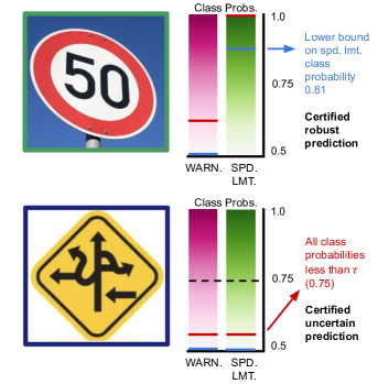
Figure 1: Certifications for a traffic sign recognition benchmark with two classes: speed limit (spd. lmt.) and warning sign (warn.). We plot original images, the upper and lower-bound class probabilities as red and blue horizontal lines, respectively, and a description of the result. Top Row: A 50 km/hr sign from the GTSRB dataset. As the lower bound class probability is 0.81, we certify that all images in the ball are classified correctly as speed limit signs and therefore no adversarial examples exist. Bottom Row: A nonsense traffic sign. As the upper bound probability for all classes is less than a threshold (0.75), we certify that the BNN is uncertain.

While retaining the advantages intrinsic to deep learning, Bayesian neural networks (BNNs), i.e., NNs with a probability distribution placed over their weights and biases [7], enable probabilistically principled evaluation of model uncertainty. Since adversarial examples are intuitively related to uncertainty [8], the application of BNNs is particularly appealing in safety-critical scenarios. In fact, model uncertainty of a BNN can, in theory, be taken into account at prediction time to enable safe decision-making [9, 10, 11, 12]. Various techniques have been proposed for the evaluation of their robustness, including generalisation of gradient-based adversarial attacks (i.e., non-Bayesian) [13], statistical verification techniques [14], as well as approaches based on pointwise (i.e., for a specific test point $x^{*}$) uncertainty evaluation [15]. However, to the best of our knowledge, a systematic approach for computing formal (i.e., with certified bounds) guarantees on the behaviour of BNNs and their decisions against adversarial input perturbations is still missing.

In this work, we develop a novel algorithmic framework to quantify the adversarial robustness of BNNs. In particular, following existing approaches for quantifying the robustness of deterministic neural networks [16, 17, 18], we model adversarial robustness as an input-output specification defined by a given compact set of input points $T\subseteq\mathbb{R}^{m}$ and a given convex polytope output set $S\subseteq\mathbb{R}^{n}$. A neural network satisfies this specification if all points in $T$ are mapped into $S$, called a safe set. Modelling specifications in this way encompasses many other practical properties such as classifier monotonicity [19] and individual fairness [20]. For a particular specification, we focus on two main properties of a BNN of interest for adversarial prediction settings: probabilistic robustness [21, 14] and decision robustness [18, 22]. The former, probabilistic robustness, is defined as the probability that a network sampled from the posterior distribution is robust (e.g., satisfies a robustness specification defined by a given $T$ and $S$). Probabilistic robustness attempts to provide a general measure of robustness of a BNN; in contrast, decision robustness focuses on the decision step, and evaluates the robustness of the optimal decision of a BNN. That is, a BNN satisfies decision robustness for a property if, for all points in $T$, the expectation of the output of the BNN in the case of regression, or the argmax of the expectation of the softmax w.r.t. the posterior distribution for classification, are contained in $S$.

Unfortunately, evaluating probabilistic and decision robustness for a BNN is not trivial, as it involves computing distributions and expectations of high-dimensional random variables passed through a non-convex function (the neural network architecture). Nevertheless, we derive a unified algorithmic framework based on computations over the BNN weight space that yields certified lower and upper bounds for both properties. Specifically, we show that probabilistic robustness is equivalent to the measure, w.r.t. the BNN posterior, of the set of weights for which the resulting deterministic NN is robust, i.e., it maps all points of $T$ to a subset of $S$. Computing upper and lower bounds for the probability involves sampling compact sets of weights according to the BNN posterior, and propagating each of these weight sets, $H$, through the neural network architecture, jointly with the input region $T$, to check whether all the networks instantiated by weights in ${H}$ are safe. To do so, we generalise bound propagation techniques developed for deterministic neural networks to the Bayesian settings and instantiate explicit schemes for Interval Bound Propagation (IBP) and Linear Bound Propagation (LBP) [23]. Similarly, in the case of decision robustness, we show that formal bounds can be obtained by partitioning the weight space into different weight sets, and for each weight set ${J}$ of the partition we again employ bound propagation techniques to compute the maximum and minimum of the decision of the NN for all input points in $T$ and different weight configurations in ${J}$. The resulting extrema are then averaged according to the posterior measure of the respective weight sets to obtain sound lower and upper bounds on decision robustness.

We perform a systematic experimental investigation of our framework on a variety of tasks. We first showcase the behaviour of our methodology on a classification problem from an airborne collision avoidance benchmark [24] and on two safety-critical industrial regression benchmarks [25]. We then consider image recognition tasks and illustrate how our method can scale to verifying BNNs on medium-sized computer vision problems, including MNIST and a two-class subset of the German Traffic Sign Recognition Benchmark (GTSRB) dataset [26]. On small networks, such as those used for airborne collision avoidance ($\sim 5000$ parameters), our method is able to verify key properties in under a second, thus enabling comprehensive certification over a fine partition of the entire state space. Moreover, when employed in conjunction with adversarial training [27], we are able to obtain non-trivial certificates for convolutional NNs (471,000 parameters) on full-colour GTSRB images (2,352 dimensions). As an example, we demonstrate the bounds on decision robustness in Figure 1, where we plot the upper and lower bound class probabilities (in red and blue respectively) for a BNN trained on a two-class traffic sign recognition benchmark. The bounds are computed for all images within a $\ell_{\infty}$ ball with radius 2/255 of the two images in the left column of the figure. For the top image of a speed limit sign, our lower bound allows us to verify that the all images within the 2/255 are correctly classified by the BNN as a 50 km/hr sign. For the bottom image of a nonsense traffic sign, our upper bound allows us to verify that the BNN is uncertain for this image and all images in the ball.

In summary, this paper makes the following contributions.

• We present an algorithmic framework based on convex relaxation techniques for the robustness analysis of BNNs in adversarial settings.

• We derive explicit lower- and upper-bounding procedures based on IBP and LBP for the propagation of input and weight intervals through the BNN posterior function.

• We empirically show that our method can be used to certify BNNs consisting of multiple hidden layers and with hundreds of neurons per layer.

A preliminary version of this paper appeared as [21]. This work extends [21] in several aspects. In contrast to [21], which focused only on probabilistic robustness, here we also tackle decision robustness and embed the calculations for the two properties in a common computational framework. Furthermore, while the method in [21] only computes lower bounds, in this paper we also develop a technique for upper bounds computation. Finally, we substantially extend the empirical evaluation to include additional datasets, evaluation of convolutional architectures and scalability analysis, as well as certification of out-of-distribution uncertainty.

II Related Work

Bayesian uncertainty estimates have been shown to empirically flag adversarial examples, often with remarkable success [28, 15]. These techniques are, however, empirical and can be circumvented by specially-tailored attacks that also target the uncertainty estimation [29]. Despite these attacks, it has been shown that BNN posteriors inferred by Hamiltonian Monte Carlo tend to be more robust to attacks than their deterministic counterparts [10]. Further, under idealised conditions of infinite data, infinitely-wide neural networks and perfect training, BNNs are provably robust to gradient-based adversarial attacks [11]. However, while showing that BNNs are promising models for defending against adversarial attacks, the arguments in [10] and [11] do not provide concrete bounds or provable guarantees for when an adversarial example does not exist for a given BNN posterior.

In [14, 9], the authors tackle similar properties of BNNs to those discussed in this paper. Yet these methods only provide bounds on probabilistic robustness and the bounds are statistical, i.e., only valid up to a user-defined, finite probability $1-\delta$, with $\delta>0$. In contrast, the method in this paper covers both probabilistic and decision robustness and computes bounds that are sound for the whole BNN posterior (i.e., hold with probability $1$). In [27], the authors incorporate worst-case information via bound propagation into the likelihood in order to train BNNs that are more adversarially robust; while that work develops a principled defense for BNNs against attack, it does not develop or study methods for analyzing or guaranteeing their robustness.

Since the publication of our preliminary work [21], the study of [30] has further investigated certifying the posterior predictive of BNNs. The definition in [30] corresponds to a subset of what we refer to as decision robustness, but their method only applies to BNNs whose posterior support has been clipped to be in a finite range. Here, we pose a more general problem of certifying decision and probabilistic robustness of BNNs, and can handle posteriors on continuous, unbounded support, which entails the overwhelming majority of those commonly employed for BNNs. Furthermore, following the preliminary version of this paper [21], [31] introduced a technique for probabilistic robustness certification implemented via a recursive algorithm the that operates over the state-space of a model-based control scenario. [32] uses similar methods to those presented in [21] to study infinite-time horizon robustness properties of BNN control policies by checking for safe weight sets and modifying the posterior so that only safe weights have non-zero posterior support.

Most existing certification methods in the literature are designed for deterministic NNs. Approaches studied include abstract interpretation [23], mixed integer linear programming [33, 34, 35, 36], game-based approaches [37, 38], and SAT/SMT [39, 24]. In particular, [40, 41, 18] employ relaxation techniques from non-convex optimisation to compute guarantees over deterministic neural network behaviours, specifically using Interval Bound Propagation (IBP) and Linear Bound Propagation (LBP) approaches. However, these methods cannot be used for BNNs because they all assume that the weights of the networks are deterministic, i.e., fixed to a given value, while in the Bayesian setting we need to certify the BNN for a continuous range of values for weights that are not fixed, but distributed according to the BNN posterior.

In the context of Bayesian learning, methods to compute adversarial robustness measures have been explored for Gaussian processes (GPs), both for regression [42] and classification tasks [43, 44]. However, because of the non-linearity in NN architectures, GP-based approaches cannot be directly employed for BNNs. Furthermore, the vast majority of approximate Bayesian inference methods for BNNs do not employ Gaussian approximations over latent space [45]. In contrast, our method is specifically tailored to take into account the non-linear nature of BNNs and can be directly applied to a range of approximate Bayesian inference techniques used in the literature.

III Background

In this section, we overview the necessary background and introduce the notation we use throughout the paper. We focus on neural networks (NNs) employed in a supervised learning scenario, where we are given a dataset of $n_{\mathcal{D}}$ pairs of inputs and labels, $\mathcal{D}=\{(x_{i},y_{i})\}_{i=1}^{n_{\mathcal{D}}}$, with $x_{i}\in\mathbb{R}^{m}$, and where each target output $y\in\mathbb{R}^{n}$ is either a one-hot class vector for classification or a real-valued vector for regression.

III-A Bayesian Deep Learning

Consider a feed forward neural network $f^{w}:\mathbb{R}^{m}\to\mathbb{R}^{n}$, parametrised by a vector $w\in\mathbb{R}^{n_{w}}$ containing all its weights and biases. We denote with $f^{w,1},...,f^{w,K}$ the $K$ layers of $f^{w}$ and take the activation function of the $i$th layer to be $\sigma^{(i)}$, abbreviated to just $\sigma$ in the case of the output activation. Throughout this paper, we will use $f^{w}(x)$ to represent pre-activation of the last layer.

Bayesian learning of deep neural network starts with a prior distribution, $p_{\mathbf{w}}(w)$, over the vector of random variables associated to the weights, $\mathbf{w}$. Placing a distribution over the weights defines a stochastic process indexed by the input space, which we denote as $f^{\mathbf{w}}$. After the data set $\mathcal{D}$ has been observed, the BNN prior distribution is updated according to the likelihood, $p(\mathcal{D}|w)=\prod_{i=1}^{n_{\mathcal{D}}}p(y_{i}|x_{i},w)$, which models how likely (probabilistically speaking) we are to observe an output under the stochasticity of our model parameters and observational noise [47]. The likelihood function, $p(y_{i}|x_{i},w)$, generally takes the shape of a softmax for multiclass classification and a multivariate Gaussian for regression. The posterior distribution over the weights given the dataset is then computed by means of the Bayes formula, i.e., $p(w|\mathcal{D})\propto p(\mathcal{D}|w)p(w)$. The cumulative distribution of $p(w|\mathcal{D})$ we denote as $P(\cdot)$, so that for $R\subseteq\mathbb{R}^{n_{w}}$ we have:

$$\int_{R}p(w|\mathcal{D})dw=P(R).$$ (1)

The posterior $p(w|\mathcal{D})$ is in turn used to calculate the output of a BNN on an unseen point, $x^{*}$. The distribution over outputs is called the posterior predictive distribution and is defined as:

$$p(y^{*}|x^{*},\mathcal{D})=\int p(y^{*}|x^{*},w)p(w|\mathcal{D})dw.$$ (2)

Equation (2) defines a distribution over the BNN output. When employing a Bayesian model, the overall final prediction is taken to be a single value, $\hat{y}$, that minimizes the Bayesian risk of an incorrect prediction according to the posterior predictive distribution and a loss function $\mathcal{L}$. Formally, the final decision of a BNN is computed as

$$\hat{y}=\operatorname*{arg\,min}_{y}\int_{\mathbb{R}^{n}}\mathcal{L}(y,y^{*})p(y^{*}|x^{*},\mathcal{D})dy^{*}.$$

This minimization is the subject of Bayesian decision theory [48], and the final form of $\hat{y}$ clearly depends on the specific loss function $\mathcal{L}$ employed in practice. In this paper, we focus on two standard loss functions widely employed for classification and regression problems.

Classification Decisions

The 0-1 loss, $\ell_{0-1}$, assigns a penalty of 0 to the correct prediction, and 1 otherwise. It can be shown that the optimal decision in this case is given by the class for which the predictive distribution obtains its maximum, i.e.:

$$\hat{y}=\operatorname*{arg\,max}_{i=1,\ldots,n}p_{i}(y^{*}|x^{*},\mathcal{D})=\operatorname*{arg\,max}_{i=1,\ldots,n}\mathbb{E}_{w\sim p(w|\mathcal{D})}\left[\sigma_{i}(f^{w}(x))\right],$$

where $\sigma_{i}$ represents the $i$th output component of the softmax function.

Regression Decisions

The $\ell_{2}$ loss assigns a penalty to a prediction according to its $\ell_{2}$ distance from the ground truth. It can be shown that the optimal decision in this case is given by the expected value of the BNN output over the posterior distribution, i.e.:

$$\hat{y}=\mathbb{E}_{w\sim p(w|\mathcal{D})}\left[f^{w}(x)\right].$$

Unfortunately, because of the non-linearity of neural network architectures, the computation of the posterior distribution over weights, $p(w|\mathcal{D})$, is generally intractable [7]. Hence, various approximation methods have been studied to perform inference with BNNs in practice. Among these methods, we will consider Hamiltonian Monte Carlo (HMC) [7] and Variational Inference (VI) [45], which we now briefly describe.

III-A1 Hamiltonian Monte Carlo (HMC)

HMC proceeds by defining a Markov chain whose invariant distribution is $p_{\mathbf{w}}(w|\mathcal{D}),$ and relies on Hamiltonian dynamics to speed up the exploration of the space. Differently from VI discussed below, HMC does not make parametric assumptions on the form of the posterior distribution, and is asymptotically correct [7]. The result of HMC is a set of samples that approximates $p_{\mathbf{w}}(w|\mathcal{D})$.

III-A2 Variational Inference (VI)

VI proceeds by finding a Gaussian approximating distribution over the weight space $q(w)\sim p_{\mathbf{w}}(w|\mathcal{D})$ in a trade-off between approximation accuracy and scalability. The core idea is that $q(w)$ depends on some hyperparameters that are then iteratively optimized by minimizing a divergence measure between $q(w)$ and $p_{\mathbf{w}}(w|\mathcal{D})$. Samples can then be efficiently extracted from $q(w)$.

For simplicity of notation, in the rest of the paper we will indicate with $p(w|\mathcal{D})$ the posterior distribution estimated by either of the two methods, and clarify the methodological differences when they arise.

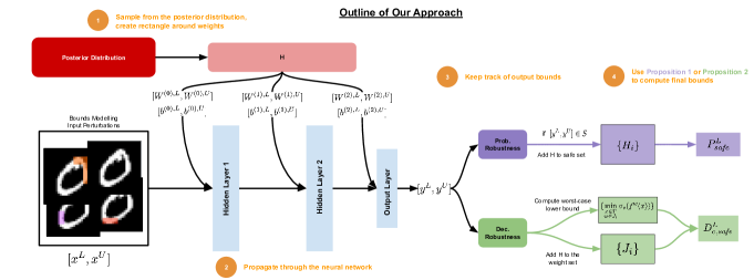
Figure 2: A diagram illustrating a single iteration of the computational flow for the certification process of a BNN w.r.t. decision robustness (green) and probabilistic robustness (purple). This process is summarised in Algorithm 1.

IV Problem Statements

We focus on local specifications defined over an input compact set $T\subseteq\mathbb{R}^{m}$ and output set $S\subseteq\mathbb{R}^{n}$ in the form of a convex polytope:

$$S=\{y\in\mathbb{R}^{n}\,|\,C_{S}y+d_{S}\geq 0\},$$ (3)

where $C_{S}\in\mathbb{R}^{n_{S}\times n}$ and $d_{S}\in\mathbb{R}^{n_{S}}$ are the matrix and vector encoding the polytope constraints, and $n_{S}$ is the number of output constraints considered. For simplicity of presentation, we assume that $T$ is defined as a box (axis-aligned linear constraints). However, we stress that all the methods in this paper can be extended to the more general case where $T$ is a convex polytope. Our formulation of input-output specifications can be used to capture important properties such as classifier monotonicity [49] and individual fairness [20], but in this work we focus exclusively on adversarial robustness. Targeted adversarial robustness, where one aims to force the neural network into a particular wrong classification, is captured in this framework by setting $T$ to be an over-approximation of an $\ell_{p}$ ball around a given test input, and setting $C_{S}$ to an $n_{S}\times n$ matrix of all zeros with a $-1$ entry in the diagonal entry corresponding to the true class and a $1$ on the diagonal entry corresponding to the target class or classes. For regression, one uses $C_{S}$ to encode the absolute deviation from the target value and $d_{S}$ to encode the maximum tolerable deviation. Throughout the paper we will refer to an input-output set pair, $T$ and $S$, as defined above as a robustness specification.

IV-A Probabilistic Robustness

Probabilistic robustness accounts for the probabilistic behaviour of a BNN in adversarial settings.

Definition 1 (Probabilistic robustness).

Given a Bayesian neural network $f^{\mathbf{w}}$, an input set $T\subseteq\mathbb{R}^{m}$ and a set $S\subseteq\mathbb{R}^{n}$ of safe outputs, then probabilistic robustness is defined as

$$P_{\text{safe}}(T,S):=Prob_{w\sim p(w|\mathcal{D})}(\forall x\in T,f^{{w}}(x)\in S).$$ (4)

Given $\eta\in[0,1]$, we then say that $f^{\mathbf{w}}$ is probabilistically robust, or safe, for specifications $T$ and $S$, with probability at least $\eta$ iff:

$$P_{\text{safe}}(T,S)\geq\eta$$

Probabilistic robustness considers the adversarial behaviour of the model while accounting for the uncertainty arising from the posterior distribution. $P_{\text{safe}}(T,S)$ represents the (weighted) proportion of neural networks sampled from $f^{\mathbf{w}}$ that satisfy a given input-output specification (captured by $T$ and $S$) and can be used directly as a measure of compliance for Bayesian neural networks. As such, probabilistic robustness is particularly suited to quantification of the robustness of a BNN to adversarial perturbations [22, 9, 50]. Exact computation of $P_{\text{safe}}(T,S)$ is hindered by both the size and non-linearity of neural networks. As $P_{\text{safe}}(T,S)$ cannot be computed exactly for general BNNs, in this work we tackle the problem of computing provable bounds on probabilistic robustness.

Problem 1 (Bounding probabilistic robustness).

Given a Bayesian neural network $f^{\mathbf{w}}$, an input set $T\subseteq\mathbb{R}^{m}$ and a set $S\subseteq\mathbb{R}^{n}$ of safe outputs, compute (non-trivial) $P_{\text{safe}}^{L}$ and $P_{\text{safe}}^{U}$ such that

$$P_{\text{safe}}^{L}\leq P_{\text{safe}}(T,S)\leq P_{\text{safe}}^{U}.$$ (5)

We highlight the difference between this problem definition and those discussed in prior works [14, 9]. In particular, prior works compute upper and lower bounds that hold with probability $1-\delta$ for some pre-specified $\delta$. While such statistical bounds can provide an estimation for $P_{\text{safe}}(T,S)$, these may not be sufficient in safety-critical contexts where strong, worst-case guarantees over the full behaviour of the BNN are necessary. The problem statement above holds with probability $1$ and represents sound guarantees on $P_{\text{safe}}(T,S)$.

IV-B Decision Robustness

While $P_{\text{safe}}$ attempts to measure the compliance of all functions in the support of a BNN posterior, we are often interested in evaluating robustness w.r.t. a specific decision. In order to do so, we consider decision robustness, which is computed over the final decision of the BNN. In particular, given a loss function and a decision $\hat{y}$ we have the following.

Definition 2 (Decision robustness).

Consider a Bayesian neural network $f^{\mathbf{w}}$, an input set $T\subseteq\mathbb{R}^{m}$ and a set $S\subseteq\mathbb{R}^{n}$ of safe outputs. Assume that the decision for a loss $\mathcal{L}$ for $x\in\mathbb{R}^{m}$ is given by $\hat{y}(x)$. Then, the Bayesian decision is considered to be robust if:

$$\forall x\in T\quad\hat{y}(x)\in S.$$ (6)

We notice that, since the specific form of the decision depends on the loss employed in practice, the definition of decision robustness takes different form depending on whether the BNN is used for classification or for regression. In particular, we instantiate the definition for the two cases of standard loss discussed in Section III.

In the regression case, using the mean square loss we have that $\hat{y}(x)=\mathbb{E}[f^{w}(x)]$, so that if we find upper and lower bounds on $\mathbb{E}[f^{w}(x)]$ for all $x\in T$, i.e., for $i=1,...,m$:

$$D_{\text{safe},i}^{L} \leq\min_{x\in T}\mathbb{E}\left[f^{w}_{i}(x)\right],\;D_{\text{safe},i}^{U}\geq\max_{x\in T}\mathbb{E}\left[f^{w}_{i}(x)\right],$$

we can then simply check whether these are within $S$.

For the classification case, where the decision is given by the $\operatorname*{arg\,max}$ of the predictive posterior, note that, in order to check the condition in Definition 2, it suffices to compute lower and upper bounds on the posterior predictive in $T$, i.e.:

$$D_{\text{safe},i}^{L} \leq\min_{x\in T}\mathbb{E}\left[\sigma_{i}(f^{w}(x))\right],\;D_{\text{safe},i}^{U}\geq\max_{x\in T}\mathbb{E}\left[\sigma_{i}(f^{w}(x))\right],$$

for $i=1,\ldots,m$. It is easy to see that the knowledge of $D_{\text{safe},i}^{L}$ and $D_{\text{safe},i}^{U}$ for all $i=1,\ldots,m$ can be used to provide guarantees of the model decision belonging to $S$, as defined in Equation (3), by simply propagating these bounds through the equations. Therefore, for both classification and regression we have to bound an expectation of the BNN output over the posterior distribution, with the additional softmax computations for classification. We thus arrive at the following problem for bounding decision robustness.

Problem 2 (Bounding decision robustness).

Let $f^{\mathbf{w}}$ be a BNN with posterior distribution $p(w|\mathcal{D})$. Consider an input-output specification ($T$, $S$) and assume $\mathcal{L}=\ell_{0-1}$ for classification or $\mathcal{L}=\ell_{2}$ for regression. We aim at computing (non-trivial) lower and upper bounds $D_{\text{safe}}^{L}$ and $D_{\text{safe}}^{U}$ such that:

$$D_{\text{safe}}^{L}\leq\mathbb{E}[s(f^{w}(x))]\leq D_{\text{safe}}^{U}\quad\forall x\in T,$$

where $s=\sigma$ for classification and $s=\mathbb{I}$ for regression.

Note that, while for regression we bound the decision directly, for classification we compute the bounds on the predictive posterior and use these to compute bounds on the final decision. This is similar to what is done for deterministic neural networks, where in the case of classification the bounds are often computed over the logit, and then used to provide guarantees for the final decision [18]. As with probabilistic robustness, our bounds on decision robustness are sound guarantees and do not have a probability of error as with statistical bounds.

IV-C Outline of our Approach:

We design an algorithmic framework for worst-case and best-case bounds on local robustness properties in Bayesian neural networks, taking account of both the posterior distribution ($P_{\text{safe}}^{L}$ and $P_{\text{safe}}^{U}$) and the overall model decision ($D_{\text{safe}}^{L}$ and $D_{\text{safe}}^{U}$). First, we show how the two robustness properties of Definitions 1 and 2 can be reformulated in terms of computation over weight intervals. This allows us to derive a unified approach to the bounding of the robustness of the BNN posterior (i.e., probabilistic robustness) and of the robustness of the overall model decision (i.e., decision robustness) that is based on bound propagation and posterior integral computation over hyper-rectangles. A visual outline for our framework is presented in Figure 2. We organise the presentation of our framework by first introducing a general theoretical framework for bounding the robustness quantities of interest (Section V). We will then show how the required integral computations can be achieved for Bayesian posterior inference techniques commonly used in practice (Section VI-A). Hence, we will show how to extend bound propagation techniques to deal with both input variable intervals and intervals over the weight space, and will instantiate approaches based on Interval and Linear Bound Propagation techniques (Section VI-B). Finally (Section VII), we will present an overall algorithm that produces the desired bounds.

V Formulating BNN Adversarial Robustness via Weight Sets

In this section, we show how a single computational framework can be leveraged to compute bounds on both definitions of BNN robustness. We start by converting the computation of robustness into weight space and then define a family of weight intervals that we leverage to bound the integrations required by both definitions. Interestingly, we find that the resulting theoretical bounds in both cases depend on the same quantities. Proofs for the main results in this section are presented in Appendix C.

V-A Bounding Probabilistic Robustness

We first show that the computation of $P_{\text{safe}}(T,S)$ is equivalent to computing a maximal set of safe weights $H$ such that each network associated to weights in $H$ is safe w.r.t. the robustness specification at hand.

Definition 3 (Maximal safe and unsafe sets).

We say that ${H}\subseteq\mathbb{R}^{n_{w}}$ is the maximal safe set of weights from $T$ to $S$, or simply the maximal safe set of weights, iff $H=\{w\in\mathbb{R}^{n_{w}}\,|\,\forall x\in T,f^{{w}}(x)\in S\}.$ Similarly, we say that ${K}\subseteq\mathbb{R}^{n_{w}}$ is the maximal unsafe set of weights from $T$ to $S$, or simply the maximal unsafe set of weights, iff $K=\{w\in\mathbb{R}^{n_{w}}\,|\,\exists\*x\in T,f^{{w}}(\*x)\not\in S\}.$

Intuitively, $H$ and $K$ simply encode the input-output specifications $S$ and $T$ in the BNN weight space. The following lemma, which trivially follows from Equation 4, allows us to directly relate the maximal sets of weights to the probability of robustness.

Lemma 1.

Let $H$ and $K$ be the maximal safe and unsafe sets of weights from $T$ to $S$. Assume that $w\sim p(w|\mathcal{D})$. Then, it holds that

$$P(H)=\int_{H}p(w|\mathcal{D})dw=P_{\text{safe}}(T,S)=$$ (7)

$$1-\int_{K}p(w|\mathcal{D})dw=1-P(K).$$

Lemma 1 simply translates the robustness specification from being concerned with the input-output behaviour of the BNN to an integration on the weight space.

An exact computation of sets $H$ and $K$ is infeasible in general. However, we can easily compute subsets of $H$ and $K$. Such subsets can then be used to compute upper and lower bounds on the value of $P_{\text{safe}}(T,S)$ by considering subsets of the maximal safe and unsafe weights.

Definition 4 (Safe and unsafe sets).

Given a maximal safe set ${H}$ or a maximal unsafe set $K$ of weights, we say that $\hat{H}$ and $\hat{K}$ are a safe and unsafe set of weights from $T$ to $S$ iff $\hat{H}\subseteq H$ and $\hat{K}\subseteq K$, respectively.

$\hat{H}$ and $\hat{K}$ can include any safe and unsafe weights, respectively, without requiring they are maximal. Without maximality, we no longer have strict equality in Lemma 1, but instead we arrive at bounds on the value of probabilistic robustness.

We proceed by defining $\hat{H}$ and $\hat{K}$ as the union of a family of disjoint weight intervals, as these can provide flexible approximations of $H$ and $K$. That is, we consider $\mathcal{H}=\{H_{i}\}_{i=1}^{n_{H}}$, with $H_{i}=[w^{L,H}_{i},w^{U,H}_{i}]$ and $\mathcal{K}=\{K_{i}\}_{i=1}^{n_{K}}$, with $K_{i}=[w^{L,K}_{i},w^{U,K}_{i}]$ such that $H_{i}\subset H$ and $K_{i}\subset K$, $\hat{H}=\bigcup_{i=1}^{n_{H}}H_{i}$, $\hat{K}=\bigcup_{i=1}^{n_{K}}K_{i}$, and $H_{i}\cap H_{j}=\emptyset$ and $K_{i}\cap K_{j}=\emptyset$, for any $i\neq j$. Hence, as a consequence of Lemma 1, and by the fact that $\hat{H}=\bigcup_{i=1}^{n_{H}}H_{i}\subset H$ and $\hat{K}=\bigcup_{i=1}^{n_{K}}K_{i}\subset K$, we obtain the following.

Proposition 1 (Bounds on probabilistic robustness).

Let $H$ and $K$ be the maximal safe and unsafe sets of weights from $T$ to $S$. Consider two families of pairwise disjoint weight intervals $\mathcal{H}=\{H_{i}\}_{i=1}^{n_{H}}$, $\mathcal{K}=\{K_{i}\}_{i=1}^{n_{K}}$ , where for all $i$:

$$H_{i}\subseteq H,\quad K_{i}\subseteq K.$$ (8)

Let $\hat{H}\subseteq H$ and $\hat{K}\subseteq K$ be non-maximal safe and unsafe sets of weights, with $\hat{H}=\bigcup_{i=1}^{n_{H}}H_{i}$ and $\hat{K}=\bigcup_{i=1}^{n_{K}}K_{i}$. Assume that $w\sim p(w|\mathcal{D})$. Then, it holds that

$$P_{\text{safe}}^{L}:=\sum_{i=1}^{n_{H}}P(H_{i})\leq P_{\text{safe}}(T,S,\mathbf{w})\leq 1-\sum_{i=1}^{n_{K}}P(K_{i})=:P_{\text{safe}}^{U},$$ (9)

that is, $P_{\text{safe}}^{L}$ and $P_{\text{safe}}^{U}$ are, respectively, lower and upper bounds on probabilistic robustness.

Through the use of Proposition 1 we can thus bound probabilistic robustness by performing computation over sets of safe and unsafe intervals. Note that the bounds are given in the case where $\mathcal{H}$ and $\mathcal{K}$ are families of pairwise disjoint weight sets. The general case can be tackled by using the Bonferroni bound, which is discussed in Appendix D-D for hyper-rectangular weight sets.

Before explaining in detail how such bounds can be explicitly computed, first, in the next section, we show how a similar derivation leads us to analogous bounds and computations for decision robustness.

V-B Bounding Decision Robustness

The key difference between our formulation of probabilistic robustness and that of decision robustness is that, for the former, we are only interested in the behaviour of neural networks extracted from the BNN posterior that satisfy the robustness requirements (hence the distinction between $H$- and $K$-weight intervals), whereas for the computation of bounds on decision robustness we need to take into account the overall worst-case behaviour of an expected value computed for the BNN predictive distribution in order to compute sound bounds. As such, rather than computing safe and unsafe sets, we only need a family of weight sets, $\mathcal{J}=\{J_{i}\}_{i=1}^{n_{J}}$, and rely on that for bounding $D_{\text{safe}}(T,S)$. We explicitly show how this can be done for classification with likelihood $\sigma$. The bound for regression follows similarly by using the identity function as $\sigma$.

Proposition 2 (Bounding decision robustness).

Let $\mathcal{J}=\{J_{i}\}_{i=1}^{n_{J}}$, with $J_{i}\subset\mathbb{R}^{n_{w}}$ be a family of disjoint weight intervals. Let $\sigma^{L}$ and $\sigma^{U}$ be vectors that lower and upper bound the co-domain of the final activation function, and $c\in\{1,\ldots,m\}$ an index spanning the BNN output dimension. Define:

$$D_{\text{safe},c}^{L}:=\sum_{i=1}^{n_{J}}P(J_{i})\min_{\begin{subarray}{c}x\in T\\ w\in J_{i}\end{subarray}} \sigma_{c}(f^{w}(x))+\sigma^{L}\left(1-\sum_{i=1}^{n_{J}}P(J_{i})\right)$$ (10)

$$D_{\text{safe},c}^{U}:=\sum_{i=1}^{n_{J}}P(J_{i})\max_{\begin{subarray}{c}x\in T\\ w\in J_{i}\end{subarray}} \sigma_{c}(f^{w}(x))+\sigma^{U}\left(1-\sum_{i=1}^{n_{J}}P(J_{i})\right).$$ (11)

Consider the vectors $D_{\text{safe}}^{L}=[D_{\text{safe},1}^{L},\ldots,D_{\text{safe},m}^{L}]$ and $D_{\text{safe}}^{U}=[D_{\text{safe},1}^{U},\ldots,D_{\text{safe},m}^{U}]$, then it holds that:

$$D_{\text{safe}}^{L}\leq\mathbb{E}_{p(w|\mathcal{D})}[\sigma(f^{w}(x))]\leq D_{\text{safe}}^{U}\quad\forall x\in T,$$

that is, $D_{\text{safe}}^{L}$ and $D_{\text{safe}}^{U}$ are lower and upper bounds on the predictive distribution in $T$.

Intuitively, the first terms in the bounds of Equations (10) and (11) consider the worst-case output for the input set $T$ and each interval $J_{i}$, while the second term accounts for the worst-case value of the posterior mass not captured by the family of intervals $\mathcal{J}$ by taking a coarse, overall bound on that region. The provided bound is valid for any family of intervals $\mathcal{J}$. Ideally, however, the partition should be finer around regions of high probability mass of the posterior distribution, as these make up the dominant term in the computation of the posterior predictive. We will discuss in Section VI how we select these intervals in practice so as to empirically obtain non-vacuous bounds.

V-C Computation of the Bounds

We now propose a unified approach to computing these lower and upper bounds. We first observe that the bounds in Equations (9), (10) and (11) require the integration of the posterior distribution over weight intervals, i.e., $P(H_{i})$, $P(K_{i})$ and $P(J_{i})$. While this is in general intractable, we have built the bound so that $H_{i}$, $K_{i}$ and $J_{i}$ are axis-aligned hyper-rectangles, and so the computation can be done exactly for approximate Bayesian inference methods used in practice. This will be the topic of Section VI-A, where, given a rectangle in weight space of the form $R=[w^{L},w^{U}]$, we will show how to compute $P(R)=\int_{R}p(w|\mathcal{D})dw$.

For the explicit computation of decision robustness, the only missing ingredient is then the computation of the minimum and maximum $\sigma(f^{w}(x))$ for $x\in T$ and $w\in J_{i}$. We do this by bounding the BNN output for any given rectangle in the weight space $R$. That is, we will compute upper and lower bounds $y^{L}$ and $y^{U}$ such that:

$$y^{L}\leq\min_{\begin{subarray}{c}x\in T\\ w\in R\end{subarray}}f^{w}(x)\quad y^{U}\geq\max_{\begin{subarray}{c}x\in T\\ w\in R\end{subarray}}f^{w}(x),$$ (12)

which can then be used to bound $\sigma(f^{w}(x))$ by simple propagation over the softmax (if needed). The derivation of such bounds will be the subject of Section VI-B.

Finally, observe that, whereas for decision robustness we can simply select any weight interval $J_{i}$, for probabilistic robustness one needs to make a distinction between safe sets ($H_{i}$) and unsafe sets ($K_{i}$). It turns out that this can be done by bounding the output of the BNN in each of these intervals. For example, in the case of the safe sets, by definition we have that $\forall w\in H_{i},\forall x^{\prime}\in T$ it follows that $f^{w}(x^{\prime})\in S$. By defining $y^{L}$ and $y^{U}$ as in Equation (12), we can see that it suffices to check whether $[y^{L},y^{U}]\subseteq S$. Hence, the computation of probabilistic robustness also depends on the computation of such bounds (again, discussed in Section VI-B).

Therefore, once we have shown how the computation of $P(R)$ for any weight interval and $y^{L}$ and $y^{U}$ can be done, the bounds in Proposition 1 and Proposition 2 can be computed explicitly, and we can thus bound probabilistic and decision robustness. Section VII will assemble these results together into an overall computational flow of our methodology.

VI Explicit Bound Computation

In this section, we provide details on the specific computations needed to calculate the theoretical bound presented in Section V for probabilistic and decision robustness. We start by discussing how a weight intervals family can be generated in practice, and how to integrate over them in Section VI-A. In Section VI-B, we then derive a scheme based on convex-relaxation techniques for bounding the output of BNNs.

VI-A Integral Computation over Weight Intervals

Key to the computation of the bounds derived in Section V is the ability to compute the integral of the posterior distribution over a combined set of weight intervals. Crucially, the shape of the weight sets $\mathcal{H}=\{H_{i}\}_{i=1}^{n_{H}}$, $\mathcal{K}=\{K_{i}\}_{i=1}^{n_{K}}$ and $\mathcal{J}=\{J_{i}\}_{i=1}^{n_{J}}$ is a parameter of the method, so that it can be chosen to simplify the integral computation depending on the particular form of the approximate posterior distribution used. We build each weight interval as an axis-aligned hyper-rectangle of the form $R=[w^{L},w^{U}]$ for $w^{L}$ and $w^{U}\in\mathbb{R}^{n_{w}}$.

Weight Intervals for Decision Robustness

In the case of decision robustness it suffices to sample any weight interval $J_{i}$ to compute the bounds we derived in Proposition 2. Clearly, the bound is tighter if the $\mathcal{J}$ family is finer around the area of high probability mass for $p(w|\mathcal{D})$. In order to obtain such a family we proceed as follows. First, we define a weight margin $\gamma>0$ that has the role of parameterising the radius of the weight intervals we define. We then iteratively sample weight vectors $w_{i}$ from $p(w|\mathcal{D})$, for $i=1,\ldots,n_{J}$, and finally define $J_{i}=[w^{L}_{i},w^{U}_{i}]=[w_{i}-\gamma,w_{i}+\gamma]$. As such, thus defined weight intervals naturally hover around the area of greater density for $p(w|\mathcal{D})$, while asymptotically covering the whole support of the distribution.

Weight Intervals for Probabilistic Robustness

On the other hand, for the computation of probabilistic robustness one has to make a distinction between safe weight intervals $H_{i}$ and unsafe ones $K_{i}$. As explained in Section V-C, this can be done by bounding the output of the BNN in each of these intervals. For example, in the case of the safe sets, by definition, $H_{i}$ is safe if and only if $\forall w\in H_{i},\forall x^{\prime}\in T$ we have that $f^{w}(x^{\prime})\in S$. Thus, in order to build a family of safe (respectively unsafe) weight intervals $H_{i}$ ($K_{i}$), we proceed as follows. As for decision robustness, we iteratively sample weights $w_{i}$ from the posterior used to build hyper-rectangles of the form $R_{i}=[w_{i}-\gamma,w_{i}+\gamma]$. We then propagate the BNN through $R$ and check whether the output of the BNN in $R$ is (is not) a subset of $S$. The derivation of such bounds on propagation will be the subject of Section VI-B.

Once the family of weights is computed, there remains the computation of the cumulative distribution over such sets. The explicit computations depend on the particular form of Bayesian approximate inference that is employed. We discuss explicitly the case of Gaussian variational approaches, and of sample-based posterior approximation (e.g., HMC), which entails the majority of the approximation methods used in practice [51].

Variational Inference

For variational approximations, $p(w|\mathcal{D})$ takes the form of a multi-variate Gaussian distribution over the weight space. The resulting computations reduce to the integral of a multi-variate Gaussian distribution over a finite-sized axis-aligned rectangle, which can be computed using standard methods from statistics [52]. In particular, under the common assumption of variational inference with a Gaussian distribution with diagonal covariance matrix [53], i.e., $p(w|\mathcal{D})=\mathcal{N}(\mu,\Sigma)$, with $\Sigma=\textrm{diag}(\Sigma_{1},\ldots,\Sigma_{n_{w}})$, we obtain the following result for the posterior integration:

$$P(R)=\int_{R} p(w|\mathcal{D})dw=$$ (13)

$$\prod_{j=1}^{n_{w}}\frac{1}{2}\left(\text{erf}\left(\frac{\mu_{j}-w^{L}_{i}}{\sqrt{2\Sigma_{j}}}\right)-\text{erf}\left(\frac{\mu_{j}-w^{u}_{i}}{\sqrt{2\Sigma_{j}}}\right)\right).$$

By plugging this into the bounds of Equation (9) for $P(H_{i})$ and $P(K_{i})$ for probabilistic robustness and in Equations (10) and (11) for decision robustness, one obtains a closed-form formula for the bounds given weight set interval families $\mathcal{H}$, $\mathcal{K}$ and $\mathcal{J}$.

Sample-based approximations

In the case of sample-based posterior approximation (e.g., HMC), we have that $p(w|\mathcal{D})$ defines a distribution over a finite set of weights. In this case we can simplify the computations by selecting the weight margin $\gamma=0$, so that each sampled interval will be of the form $R=[w_{i},w_{i}]$ and its probability under the discrete posterior will trivially be:

$$P(R_{i})=p(w_{i}|\mathcal{D}).$$ (14)

VI-B Bounding Bayesian Neural Networks’ Output

Given an input specification, $T$, and a weight interval, $R=[w^{L},w^{U}]$, the second key step in computing probabilistic and decision robustness is the bounding of the output of the BNN over $R$ given $T$. That is, we need to derive methods to compute $[y^{L},y^{U}]$ such that, by construction, $\forall w\in[w^{L},w^{U}],\forall x^{\prime}\in T$ it follows that $f^{w}(x^{\prime})\in[y^{L},y^{U}]$.

In this section, we discuss interval bound propagation (IBP) and linear bound propagation (LBP) as methods for computing the desired output set over-approximations. Before discussing IBP and LBP in detail, we first introduce common notation for the rest of the section. We consider feed-forward neural networks of the form:

$$z^{(0)} =x$$ (15)

$$\zeta^{(k+1)}_{i} =\sum_{j=1}^{n_{k}}W^{(k)}_{ij}z^{(k)}_{j}+b^{(k)}_{i}\quad i=0,\ldots,n_{k+1}$$ (16)

$$z^{(k)}_{i} =\sigma(\zeta^{(k)}_{i})\qquad\qquad\qquad i=0,\ldots,n_{k}$$ (17)

for $k=1,\ldots,K$, where $K$ is the number of hidden layers, $\sigma(\cdot)$ is a pointwise activation function, $W^{(k)}\in\mathbb{R}^{n_{k}\times n_{k-1}}$ and $b^{(k)}\in\mathbb{R}^{n_{k}}$ are the matrix of weights and vector of biases that correspond to the $k$th layer of the network and $n_{k}$ is the number of neurons in the $k$th hidden layer. Note that, while Equations (15)–(17) are written explicitly for fully-connected layers, convolutional layers can be accounted for by embedding them in fully-connected form [41].

We write $W^{(k)}_{i:}$ for the vector comprising the elements from the $i$th row of $W^{(k)}$, and similarly $W^{(k)}_{:j}$ for that comprising the elements from the $j$th column. $\zeta^{(K+1)}$ represents the final output of the network (or the logit in the case of classification networks), that is, $\zeta^{(K+1)}=f^{w}(x)$. We write $W^{(k),L}$ and $W^{(k),U}$ for the lower and upper bound induced by $R$ for $W^{(k)}$ and $b^{(k),L}$ and $b^{(k),U}$ for those of $b^{(k)}$, for $k=0,\ldots,K$. Observe that $z^{(0)}$, $\zeta^{(k+1)}_{i}$ and $z^{(k)}_{i}$ are all functions of the input point $x$ and of the combined vector of weights $w=[W^{(0)},b^{(0)},\ldots,W^{(K)},b^{(K)}]$. We omit the explicit dependency for simplicity of notation. Finally, we remark that, as both the weights and the input vary in a given set, Equation (16) defines a quadratic form.

Interval Bound Propagation (IBP)

IBP has already been employed for fast certification of deterministic neural networks [18]. For a deterministic network, the idea is to propagate the input box around $x$, i.e., $T=[x^{L},x^{U}]$, through the first layer, so as to find values $z^{(1),L}$ and $z^{(1),U}$ such that $z^{(1)}\in[z^{(1),L},z^{(1),U}]$, and then iteratively propagate the bound through each consecutive layer for $k=1,\ldots,K$. The final box constraint in the output layer can then be used to check for the specification of interest [18]. The only adjustment needed in our setting is that at each layer we also need to propagate the interval of the weight matrix $[W^{(k),L},W^{(k),U}]$ and that of the bias vector $[b^{(k),L},b^{(k),U}]$. This can be done by noticing that the minimum and maximum of each term of the bi-linear form of Equation (16), that is, of each monomial $W^{(k)}_{ij}z^{(k)}_{j}$, lies in one of the four corners of the interval $[W^{(k),L}_{ij},W^{(k),U}_{ij}]\times[z^{(k),L}_{j},z^{(k),U}_{j}]$, and by adding the minimum and maximum values respectively attained by $b^{(k)}_{i}$. As in the deterministic case, interval propagation through the activation function proceeds by observing that generally employed activation functions are monotonic, which permits the application of Equation (17) to the bounding interval. Where monotonicity does not hold, we can bound any activation function that has finitely many inflection points by splitting the function into piecewise monotonic functions. This is summarised in the following proposition.

Proposition 3.

Let $f^{w}(x)$ be the network defined by the set of Equations (15)–(17), let for $k=0,\ldots,K$:

$$t_{ij}^{(k),L}=\min \{W_{ij}^{(k),L}z_{j}^{(k),L},W_{ij}^{(k),U}z_{j}^{(k),L},$$

$$W_{ij}^{(k),L}z_{j}^{(k),U},W_{ij}^{(k),U}z_{j}^{(k),U}\}$$

$$t_{ij}^{(k),U}=\max \{W_{ij}^{(k),L}z_{j}^{(k),L},W_{ij}^{(k),U}z_{j}^{(k),L},$$

$$W_{ij}^{(k),L}z_{j}^{(k),U},W_{ij}^{(k),U}z_{j}^{(k),U}\}$$

where $i=1,\ldots,n_{k+1}$, $j=1,\ldots,n_{k}$, and $z^{(k),L}=\sigma(\zeta^{(k),L})$, $z^{(k),U}=\sigma(\zeta^{(k),U})$ and:

$$\zeta^{(k+1),L} =\sum_{j}t_{:j}^{(k),L}+b^{(k),L}$$

$$\zeta^{(k+1),U} =\sum_{j}t_{:j}^{(k),U}+b^{(k),U}.$$

Then we have that $\forall x\in T$ and $\forall w\in R$:

$$f^{w}(x)=\zeta^{(K+1)}\in\left[\zeta^{(K+1),L},\zeta^{(K+1),U}\right].$$

The proposition above, whose proof is Appendix C-C (Appendix C subsection C), yields a bounding box for the output of the neural network in $T$ and $R$.

Linear Bound Propagation (LBP)

We now discuss how LBP can be used to lower-bound the BNN output over $T$ and $R$ as an alternative to IBP. In LBP, instead of propagating bounding boxes, one finds lower and upper Linear Bounding Functions (LBFs) for each layer and then propagates them through the network. As the bounding function has an extra degree of freedom w.r.t. the bounding boxes obtained through IBP, LBP usually yields tighter bounds, though at an increased computational cost. Since in deterministic networks non-linearity comes only from the activation functions, LBFs in the deterministic case are computed by bounding the activation functions, and propagating the bounds through the affine function that defines each layer.

Similarly, in our setting, given $T$ in the input space and $R$ for the first layer in the weight space, we start with the observation that LBFs can be obtained and propagated through commonly employed activation functions for Equation (17), as discussed in [41].

Lemma 2.

Let $f^{w}(x)$ be defined by Equations (15)–(17). For each hidden layer $k=1,\ldots,K$, consider a bounding box in the pre-activation function, i.e. such that $\zeta^{(k)}_{i}\in[\zeta^{(k),L}_{i},\zeta^{(k),U}_{i}]$ for $i=1,\ldots,n_{k}$. Then there exist coefficients $\alpha^{(k),L}_{i}$, $\beta^{(k),L}_{i}$, $\alpha^{(k),U}_{i}$ and $\beta^{(k),U}_{i}$ of lower and upper LBFs on the activation function such that for all $\zeta^{(k)}_{i}\in[\zeta^{(k),L}_{i},\zeta^{(k),U}_{i}]$ it holds that:

$$\alpha^{(k),L}_{i}\zeta^{(k)}_{i}+\beta^{(k),L}_{i}\leq\sigma(\zeta^{(k)}_{i})\leq\alpha^{(k),U}_{i}\zeta^{(k)}_{i}+\beta^{(k),U}_{i}.$$

The lower and upper LBFs can thus be minimised and maximised to propagate the bounds of $\zeta^{(k)}$ in order to compute a bounding interval $[z^{(k),L},z^{(k),U}]$ for $z^{(k)}=\sigma(\zeta^{(k)})$. Then, LBFs for the monomials of the bi-linear form of Equation (16) can be derived using McCormick’s inequalities [54]:

$$W_{ij}^{(k)}z_{j}^{(k)}\geq W_{ij}^{(k),L}z^{(k)}_{j}+W_{ij}^{(k)}z^{(k),L}_{j}-W_{ij}^{(k),L}z^{(k),L}_{j}$$ (18)

$$W_{ij}^{(k)}z_{j}^{(k)}\leq W_{ij}^{(k),U}z^{(k)}_{j}+W_{ij}^{(k)}z^{(k),L}_{j}-W_{ij}^{(k),U}z^{(k),L}_{j}$$ (19)

for every $i=1,\ldots,n_{k}$, $j=1,\ldots,n_{k-1}$ and $k=1,\ldots,K$. The bounds of Equations (18)–(19) can thus be used in Equation (16) to obtain LBFs on the pre-activation function of the following layer, i.e. $\zeta^{(k+1)}$. The final linear bound can be obtained by iterating the application of Lemma 2 and Equations (18)–(19) through every layer. This is summarised in the following proposition, which is proved in Appendix C along with an explicit construction of the LBFs.

Proposition 4.

Let $f^{w}(x)$ be the network defined by the set of Equations (15)–(17). Then for every $k=0,\ldots,K$ there exists lower and upper LBFs on the pre-activation function of the form:

$$\zeta^{(k+1)}_{i}\geq\mu_{i}^{(k+1),L}\cdot x+\sum_{l=0}^{k-1}\langle\nu_{i}^{(l,k+1),L},W^{(l)}\rangle+$$

$$\nu_{i}^{(k,k+1),L}\cdot W^{(k)}_{i:}+\lambda_{i}^{(k+1),L}\quad\textrm{for}\;i=1,\ldots,n_{k+1}$$

$$\zeta^{(k+1)}_{i}\leq\mu_{i}^{(k+1),U}\cdot x+\sum_{l=0}^{k-1}\langle\nu_{i}^{(l,k+1),U},W^{(l)}\rangle+$$

$$\nu_{i}^{(k-1,k+1),U}\cdot W^{(k)}_{i:}+\lambda_{i}^{(k+1),U}\quad\textrm{for}\;i=1,\ldots,n_{k+1}$$

where $\langle\cdot,\cdot\rangle$ is the Frobenius product between matrices, $\cdot$ is the dot product between vectors, and the explicit formulas for the LBF coefficients, i.e., $\mu_{i}^{(k+1),L}$, $\nu_{i}^{(l,k+1),L}$, $\lambda_{i}^{(k+1),L}$, $\mu_{i}^{(k+1),U}$, $\nu_{i}^{(l,k+1),U}$, are given in Appendix C-D.

Now let $\zeta^{(k),L}_{i}$ and $\zeta^{(k),U}_{i}$, respectively, be the minimum and the maximum of the right-hand side of the two equations above; then we have that $\forall x\in T$ and $\forall w\in R$:

$$f^{w}(x)=\zeta^{(K+1)}\in\left[\zeta^{(K+1),L},\zeta^{(K+1),U}\right].$$

Algorithm 1 Lower Bounds for BNN Probabilistic Robustness

Input: $T$ – Input Region, $f^{\mathbf{w}}$ – Bayesian Neural Network, $p(w|\mathcal{D})$ – Posterior Distribution with variance $\Sigma$, $N$ – Number of Samples, $\gamma$ – Weight margin.
Output: A sound lower bound on $P_{\text{safe}}(T,S)$.  

1:   # $\mathcal{H}$ is a set of known safe weight intervals

2:  $\mathcal{H}\leftarrow\emptyset$

3:   # Elementwise product to obtain width of weight margin

4:  $v\leftarrow\gamma\cdot I\cdot\Sigma$

5:  for $i\leftarrow 0$ to $N$ do

6:     $w^{(i)}\sim p(w|\mathcal{D})$

7:      # Assume weight intervals are built to be disjoint

8:     $[w^{(i),L},w^{(i),U}]\leftarrow[w_{i}-v,w_{i}+v]$

9:      # Interval/Linear Bound Propagation, Section VI-B

10:     $\*y^{L},\*y^{U}\leftarrow\texttt{Propagate}(f,T,[w^{(i),L},w^{(i),U}]$)

11:     if $[\*y^{L},\*y^{U}]\subset S$ then

12:        $\mathcal{H}\leftarrow\mathcal{H}\bigcup\{[w^{(i),L},w^{(i),U}]\}$

13:     end if

14:  end for

15:  $P_{\text{safe}}^{L}\leftarrow 0.0$

16:  for $[w^{(i),L},w^{(i),U}]\in\mathcal{H}$ do

17:      # Compute safe weight probs, Section VI-A

18:     $P_{\text{safe}}^{L}=P_{\text{safe}}^{L}+P([w^{(i),L},w^{(i),U}])$

19:  end for

20:  return $P_{\text{safe}}^{L}$

VII Complete Bounding Algorithm

Using the results presented in Section VI, it is possible to explicitly compute the bounds on probabilistic and decision robustness derived in Section V. In this section, we bring together all the results discussed so far, and assemble complete algorithms for the computation of bounds on $P_{\text{safe}}(T,S)$ and $D_{\text{safe}}(T,S)$. We discuss the procedure to lower bound $P_{\text{safe}}(T,S)$ in Algorithm 1. We then discuss the details of upper bounds and bounds on $D_{\text{safe}}(T,S)$, leaving the algorithms and their description for these bounds to Appendix D.

VII-A Lower Bounding Algorithm

We provide a step-by-step outline for how to compute lower bounds on $P_{\text{safe}}(T,S)$ in Algorithm 1. We start on line 2 by initializing the family of safe weight sets $\mathcal{H}$ to be the empty set and by scaling the weight margin with the posterior weight scale (line 4). We then iteratively (line 5) proceed by sampling weights from the posterior distribution (line 6), building candidate weight boxes (line 8), and propagate the input and weight box through the BNN (line 10). We next check whether the propagated output set is inside the safe output region $S$, and if so update the family of weights $\mathcal{H}$ to include the weight box currently under consideration (lines 11 and 12). Finally, we rely on the results in Section VI-A to compute the overall probabilities over all the weight sets in $\mathcal{H}$, yielding a valid lower bound for $P_{\text{safe}}(T,S)$. For clarity of presentation, we assume that all the weight boxes that we sample in lines 6–8 are pairwise disjoint, as this simplifies the probability computation. The general case with overlapping weight boxes relies on the Bonferroni bound and is given in Appendix D-D. The algorithm for the computation of the lower bound on $D_{\text{safe}}(T,S)$ (listed in the Appendix D as Algorithm 2) proceeds in an analogous way, but without the need to perform the check in line 11, and by adjusting line 18 to the formula from Proposition 2.

VII-B Upper Bounding Algorithm

Upper bounding $P_{\text{safe}}(T,S)$ and $D_{\text{safe}}(T,S)$ follows the same computational flow as Algorithm 1. The pseudocode outlines computation of probabilistic and decision robustness are listed respectively in Algorithm 3 and 4 in Appendix D subsection A and Appendix D subsection B. We again proceed by sampling a rectangle around weights, propagate bounds through the NN, and compute the probabilities of weight intervals. The key change to the algorithm to allow upper bound computation involves computing the best case, rather than the worst case, for $y$ in for decision robustness (line 12 in Algorithm 3) and ensuring that the entire interval $[y^{L},y^{U}]\notin S$ (line 18) for probabilistic robustness. In Appendix D subsection B we also discuss how adversarial attacks can be leveraged to improve the upper bounds.

VII-C Computational Complexity

Calculations for probabilistic robustness and decision robustness follow the same computational flow and include: bounding of the neural network output, sampling from the posterior distribution, and computation of integrals over boxes on the input and weight space.

Regarding Algorithm 1 (or equivalently Algorithm 2 for decision robustness), it is clear that the computational complexity scales linearly with the number of samples, $N$, taken from the posterior distribution. Observe that, in order to obtain a tight bound on the integral computation, $N$ needs to be large enough such that $N$ samples of the posterior with width $\gamma$ span an area of high probability mass for $p(w|\mathcal{D})$. Unfortunately, this means that, for a given approximation error magnitude, $N$ needs to scale quadratically on the number of hidden neurons. Given the sampling of the hyper-rectangles, computation of the integral over the weight boxes is done through Equations (13) and (14). The integration over the weight boxes is done in constant time for HMC (though a good quality HMC posterior approximation scales with the number of parameters) and $\mathcal{O}(n_{w})$ for VI. The final step needed for the methodology is that of bound propagation, which clearly differs when using IBP or LBP. In particular, the cost of performing IBP is $\mathcal{O}(K\hat{n}\hat{m})$, where $K$ is the number of hidden layers and $\hat{n}\times\hat{m}$ is the size of the largest weight matrix $W^{(k)}$, for $k=0,\ldots,K$. LBP is, on the other hand, $\mathcal{O}(K^{2}\hat{n}\hat{m})$. Overall, the time complexity for certifying a VI BNN with IBP is therefore $\mathcal{O}(Nn_{w}K\hat{n}\hat{m})$, and similar formulas can be obtained for alternative combinations of inference and propagation techniques that are employed. We remark that, while sound, the bounds we compute are not guaranteed to converge to the true values of $P_{\text{safe}}(T,S)$ and $D_{\text{safe}}(T,S)$ in the limit of the number of sample $N$ because of the introduction of over-approximation errors due to bound propagation.

VIII Experiments

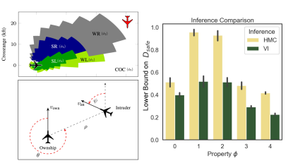
Figure 3: Top Left: Encounter geometry, ground truth and property labels: Clear of Conflict (COC), Strong Left/Right (SL/R), Weak Left/Right (WL/R), for a collision scenario. Diagrams modified from [24]. Bottom Left: Encounter geometry labelled with features used for collision avoidance prediction. Right: Bounds on decision robustness obtained for HMC and VI trained BNNs for each property.

In this section, we empirically investigate the suitability of our certification framework for the analysis of probabilistic and decision robustness in BNNs. We focus our analysis on four different case studies. First, we provide a comprehensive evaluation of an airborne collision avoidance system [24]. To do so, we partition the entire input space into 1.8 million different specifications and bound $P_{\text{safe}}(T,S)$ and $D_{\text{safe}}(T,S)$ by computing the bounds for each specification. We then turn our attention to an industrial regression benchmark [25] and demonstrate how our analysis can provide tight characterization of the worst-case error of predictions in adversarial settings in relation to the magnitude of the maximum attack allowed. Next, we analyse the scalability of our method in the well-known MNIST dataset for handwritten digits recognition [55], along with its behaviour on out-of-distribution input samples. Finally, we we study a two-class subset of the German Traffic Sign Recognition Benchmark (GTSRB) dataset [26], whose input space is 1500 dimensions larger than what has previously been studied for BNN certification against adversarial examples, showcasing that we are still able to compute non-trivial guarantees in this setting. For each dataset, we first describe the problem setting and BNN used to solve it, along with its hyperparameters. We then discuss the properties of interest for each dataset. Finally, we provide discussion and illustration of our bounds performance. All the experiments have been run on 4 NVIDIA 2080Ti GPUs in conjunction with 4 24-core Intel Core Xeon 6230.

VIII-A Airborne Collision Avoidance

Our first case study is the Horizontal airborne Collision Avoidance System (HCAS) [24], a dataset composed of millions of labelled examples of intruder scenarios.

VIII-A1 Problem Setting

The task of the BNN is to predict a turn advisory for an aircraft given another oncoming aircraft, including clear of conflict (COC), weak left (WL), weak right (WR), strong left (SL), and strong right (SR). These are depicted in the top left of Figure 3. We follow the learning procedure described in [24], where encounter scenarios are partitioned into 40 distinct datasets. We then learn a BNN to predict the correct advisories for each dataset, resulting in 40 different BNNs which need to be analysed.

To analyze the system of 40 BNNs, we first discretize the entire state-space into 1.8 million mutually exclusive input specifications. The input specifications are sized according to the spacing of the ground truth labels supplied by [24]. Namely, we consider an $\ell_{\infty}$ norm ball with different widths for each input dimension. Those widths are $[0.016,0.025,0.025,0.05]$. The output specification is taken to be the set of all softmax vectors such that the argmax of the softmax corresponds to the true label. We separate these output specifications into 5 different properties, which we termed $\phi_{j}$ for $j=0,\ldots,4$ corresponding to each of the possible advisories. For all properties in this section we use LBP with 5 samples with a weight margin of 2.5 standard deviations.

We train BNNs with Variational Online Gauss Newton (VOGN), where the posterior approximation is a diagonal covariance Gaussian, and wih Hamiltonian Monte Carlo (HMC). The BNN architecture has a single hidden layer with 125 hidden units, the same size as the original system proposed in [24]. We use a diagonal covariance Gaussian prior with variance 0.5 for VOGN and a prior variance of 2.5 for HMC.

TABLE I: Certification of airborne collision avoidance over a complete partition of the input space. Each state is either certified safe, unsafe, or not certifiable with the chosen thresholds. Number of states and proportions are reported along with the number of BNNs involved in the system for each property.

	Total Inputs	# Certified Safe ($P_{\text{safe}}(T,S)>0.98$)	# Certified Unsafe ($P_{\text{safe}}(T,S)<0.05$)	# Uncertifiable	# BNNs
$\phi_{0}$	795,853	620,158 (77.9%)	168,431 (21.1%)	7,313 (0.9%)	35
$\phi_{1}$	324,443	257,453 (79.3%)	34,379 (10.5%)	32,639 (10.0%)	21
$\phi_{2}$	323,175	257,724 (79.7%)	36,839 (11.3%)	28,612 (8.8%)	21
$\phi_{3}$	178,853	101,346 (53.4%)	64,618 (34.0%)	23,799 (12.5%)	31
$\phi_{4}$	189,991	104,546 (55.0%)	70,310 (37.0%)	15,135 (7.9%)	31
Total:	1,812,315	1,341,227 (74.0%)	374,577 (20.6%)	107,498 (5.9%)	40

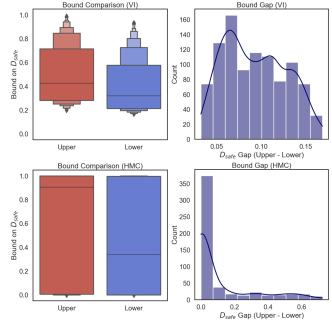
Figure 4: Left: Box plots showing the distribution of upper and lower bounds for VI (top) and HMC (bottom). Right: Histograms showing gap between upper and lower bounds for VI (top) and HMC (bottom).

VIII-A2 Analysis with $P_{\text{safe}}(T,S)$ Certification

For each of the 1.8 million disjoint input specification, we compute both upper and lower bounds on $P_{\text{safe}}(T,S)$. Given that probabilistic robustness is a real-valued probability and not a binary predicate, practitioners must select thresholds that reflect a strong belief that a value is safe or unsafe. We call these thresholds $\tau_{\text{safe}}$ and $\tau_{\text{unsafe}}$. Once one has computed bounds on $P_{\text{safe}}(T,S)$, the proportions of safe and unsafe states (as reported in Table I) can be computed by checking thresholds. We check our bounds against strict safety and unsafety thresholds $\tau_{\text{safe}}=0.98,\tau_{\text{unsafe}}=0.05$.

For the selected threshold values, Table I reports the certified performance of the BNN system. Such a report can be used by regulators and practitioners to determine the if the system is safe for deployment. In this case, we find that across all properties 74% of the states are certified to be safe while 20% are certified to be unsafe. The remaining 6% fall somewhere in between the two safety thresholds. These statistics indicate that roughly 18% of the decisions issued by the system were correct but not robust, thus the systems accuracy of 92% does not paint the complete story of its performance. Moreover, we break down each of the properties of the system, represented by each row of Table I, to understand where the most common failure modes occur. We find that the most unsafe indicators are the strong left, $\phi_{3}$, and for strong right, $\phi_{4}$, the system has the lowest certified safety at 53.4% and 55.0% respectively. They also have the highest certified unsafety at 34.0% and 37.0%, respectively. We conjecture that these these specifications are less safe due to the fact that their is less labeled data representing them in the dataset. Less data has been shown to be correlated with less robustness for BNNs [10]. If the results in Table I are deemed to be insufficient for deployment, then practitioners can collect more data for unsafe properties e.g., $\phi_{3}$ and $\phi_{4}$, or could resort to certified safe training for BNNs as suggested in [27].

VIII-A3 Analysis with $D_{\text{safe}}(T,S)$ Certification

In order to analyze the decision robustness of the BNNs, we again discretize the input space. For these results, we use a coarser discretization, with the input specification being an $\ell_{\infty}$ ball radius of $0.125$ over each input dimension, and for the sake of computational efficiency we allow some gaps between the input specifications. For each specification, we compute upper and lower bounds on $D_{\text{safe}}(T,S)$. We plot the result of our bounds on decision robustness in Figures 3 and 4. In the right hand portion of Figure 3 we visualize the average lower bound on decision robustness for two BNNs, one trained with HMC (yellow) and the other trained with VI (green). We find that we are able to certify a higher lower bound, indicating heightened robustness, for the HMC-trained BNN. This corroborates previous robustness studies that highlight that HMC is more adversarially robust [10, 11]. In Figure 4 we analyze the tightness of our bounds in this scenario by comparing the lower and upper bounds provided by our method. For VI, the gap, plotted in purple in the upper right, is tightly centered around a mean of $0.08$, with maximum gap observed in these experiments being approximately $0.16$ and a minimum $0.035$. For HMC, on the other hand, the mean gap is $0.11$, which is higher than VI, but this mean is affected by a small proportion of inputs that have a very high gap between upper and lower bounds, with the highest gap being $0.72$. We further highlight the higher variance bound distribution for the HMC-trained BNN (plotted as blue and red box plots). We hypothesize that this arises due to the higher uncertainty predictive of the HMC in areas of little data [7]

VIII-A4 Computational Requirements

For VI certification, we can compute upper and lower bounds in an average of 0.544 seconds. Thus, when run in serial mode, the 3.6 million probabilistic bound computations needed for Table I takes an estimated 11.347 computational days. However, our parallelized certification procedure produces Table I in under 3 days of computational time (61 hours). These computations include the 1.8 million lower bound runs and 1.8 million upper bound runs. For HMC, on the other hand, certification can be done in a fraction of the time, with bounds being computed in 0.073 seconds. This is due to the fact that weight intervals for HMC necessarily satisfy the pairwise disjoint precondition of Proposition 1, thus no Bonferroni correction is needed.

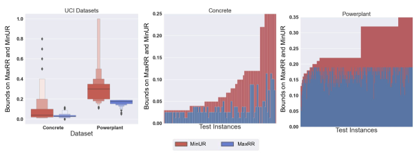
Figure 5: Computation of the minimum (MinUR) and maximum (MaxRR) safe radius for Concrete and Powerplant datasets. Left: Boxplots for the empirical distribution of MinUR and MaxRR computed over all test inputs. Centre: Per-test-instance certified radii for the Concrete dataset. Right: Per-test-instance certified radii for the Powerplant dataset.

VIII-B Industrial Benchmarks

We now focus our analyses on two safety-critical industrial regression problems taken from the UCI database [25], and widely employed for benchmarking of Bayesian inference methods [56, 57, 53].

VIII-B1 Problem Setting

The Concrete dataset involves predicting the compressive strength of concrete, based on 8 key factors including its ingredients and age. The Powerplant dataset uses six years worth of observations from combined cycle power plants and poses the problem of predicting energy output from a plant given a range of environmental and plant parameters. For each dataset we learn a BNN by using the architecture (i.e., a single hidden layer with 100 hidden units) and inference settings proposed in [53]. The BNNs are inferred using VOGN with a diagnonal covariance prior over the weights with variance 0.5 for the Concrete dataset and 0.25 for the Powerplant dataset. We use a Gaussian likelihood corresponding to a mean squarred error loss function. In this setting we use IBP with 10 samples and a weight margin of 2 standard deviations.

VIII-B2 Analysis with $P_{\text{safe}}(T,S)$ Certification

In industrial applications it is useful to understand the maximum amount of adversarial noise that a learned system can tolerate, as failures can be costly and unsafe [58]. To this end, we introduce the maximum and minimum robust radius. Given a threshold $\tau_{\text{safe}}$ (as before) the maximum robust radius (MaxRR) is the largest $\ell_{\infty}$ radius for which we can certify the BNN satisfies $P_{\text{safe}}(T,S)>\tau_{\text{safe}}$. Similarly, the minimum unrobust radius (MinUR) is the smallest radius such that we can certify $P_{\text{safe}}(T,S)<\tau_{\text{unsafe}}$. The MaxRR gives us a safe lower bound on the amount of adverarial noise a BNN is robust against, whereas the MinUR gives us a corresponding upper bound.

In our experiments on these datasets we considered $\tau_{\text{safe}}=\tau_{\text{unsafe}}=0.7$, meaning that we request that over $70\%$ of the BNN probability mass is certifiably safe; however, we stress that similar results can be obtained for different values of $\tau_{\text{safe}}$ similarly to what is discussed in our previous analysis of the HCAS dataset. In order to compute the MaxRR we start with $\epsilon=0$, check that $P_{\text{safe}}(T,S)>\tau_{\text{safe}}$ using our lower bound, and if the inequality is satisfied we increase epsilon by 0.01 and continue this process until the inequality no longer holds. Similarly for the MinUR, we start with $\epsilon=0.5$ and iteratively decrease the value of $\epsilon$ until the upper bound no longer certifies that $P_{\text{safe}}(T,S)<\tau_{\text{unsafe}}$; if the property does not hold at $0.5$ one can increase the value of $\epsilon$ until the bound holds.

The result of computing the MaxRR and MinUR over the test datasets for the Concrete and Powerplant datasets are plotted in Figure 5. We highlight that in the overwhelming majority of the cases our methods is able to return non-vacuous bounds on MinUR (i.e., strictly less than $1$) and on MaxRR (i.e., strictly greater than $0$). As expected we observe the MaxRR is strictly smaller than MinUR. Encouragingly, as MinUR grows, MaxRR tends to increase indicating that our bounds track the true value of $P_{\text{safe}}(T,S)$. We see that the Concrete dataset is typically guaranteed to be robust for radius $\epsilon\approx 0.03$ and is typically guaranteed to be unsafe for $\epsilon\approx 0.06$. For the Powerplant posterior we compute a MaxRR of roughly $0.18$ for most inputs and a MinUR lower than $0.32$. Notice how the results for the Concrete datasets systematically display more robustness than those for Powerplant and the gap between MaxRR and MinUR is significantly smaller in the former datasets than in the latter.

VIII-B3 Computational Requirements

On average, it takes 1.484 seconds to compute a certified upper or lower bound on $P_{\text{safe}}(T,S)$ for the Powerplant dataset and 1.718 seconds for the Concrete dataset. We use a linear search in order to compute the MaxRR and MinUR which require, on average, 5 certifications for both MaxRR and MinUR computations. We compute these values over the entire test datasets for both Powerplant and Concrete, which requires tens of thousands of certifications and each input can be done in parallel.

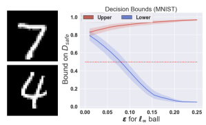
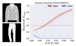
Figure 6: Left: Mean and standard deviation of upper and lower bounds obtained on $D_{\text{safe}}$ on 1000 images taken from the MNIST test set. Right: Mean and standard deviation on upper and lower bound on decision robustness on out-of-distribution samples taken from the FashionMNIST dataset.

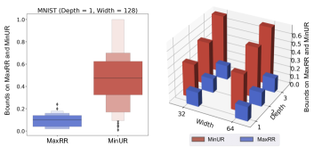
Figure 7: Left: Boxplots for the empirical distribution of the maximum safe radius and minimum unsafe radius for a BNN with 128 hidden units and a single hidden layer. Right: For a range of architectures, we plot the mean certified safe and unsafe radius.

VIII-C MNIST

We investigate the suitability of our methods in providing certifications for BNNs on larger input domains, specifically BNNs learnt for MNIST, a standard benchmark for the verification of deterministic neural networks whose inputs are 784-dimensional. In this setting we use IBP with 5 weight samples with a weight margin of 2.5 standard deviations.

VIII-C1 Problem Setting

MNIST poses the problem of handwritten digit recognition. Given handwritten digits encoded as a 28 by 28 black and white image, the task is to predict which digit – 0 through 9 – is depicted in the image (two images randomly sampled from the dataset are reproduced in the far left of Figure 6). We learn BNNs using the standard 50,000/10,000 train/test split that is provided in the original work [55]. For our experimental analysis, we use one-layer neural network with 128 hidden neurons, each of which uses rectified linear unit activation functions. The BNN has 10 output neurons that use a softmax activation function. We train the network using VOGN with a diagonal covariance Gaussian prior that has variance 2.0. We use a sparse categorical cross-entropy loss modified with the method presented in [27] to promote robustness in the BNN posteriors.

VIII-C2 Analysis using $D_{\text{safe}}(T,S)$ Certification

We analyze the trained BNN using decision robustness on 1000 images taken from the MNIST test dataset. We compute bounds on $D_{\text{safe}}(T,S)$ for increasing widths of an $\ell_{\infty}$ input region $\epsilon$. We plot the mean and standard deviation obtained for the upper ($D_{\text{safe}}^{U}$, in red) and lower bound ($D_{\text{safe}}^{L}$, in blue) on decision robustness for the ground truth label of each image in the left hand portion of Figure 6. As greater $\epsilon$ implies a larger input specification $T$, increasing values of $\epsilon$ leads to a widening of the gap between the lower and upper bounds, and hence an increased vulnerability of the network. Notice that even for $\epsilon=0.25$, i.e., half of the whole input space, our method still obtains on average non-vacuous bounds (i.e., strictly within $(0,1)$). In order to get a rough estimation of the adversarial robustness of the network, we observe that, for lower bound values above $0.5$, the BNN is guaranteed to correctly classify all the inputs in the region $T$ (however, as MNIST has 10 classes, even values of the lower bound lower than $0.5$ could still result in correct classification). Using the $0.5$ threshold, we notice that our method guarantees that the BNN is still robust on average for $\epsilon=0.075$. Notice that this is on par with results obtained for verification of deterministic neural networks, where $\epsilon=0.05$ leads to adversarial attack robustness of around $70\%$ [17].

VIII-C3 Certification of Uncertainty Behaviour

In this section we study how to certify the uncertainty behavior of a BNN in the presence of adversarial noise. We assume we have an out-of-distribution input, i.e., an input whose ground-truth does not belong to any of the classes in the range of the learned model. As with previous specifications, we build the set $T$ around such an input with an $\ell_{\infty}$ ball of radius $\epsilon$. Unlike for the previous specifications, we build $S$ as the set of all softmax vectors such that no entry in the vector is larger than a specified value $\tau_{\text{uncertain}}$. The function of $\tau_{\text{uncertain}}$ is to determine the confidence at which a classification is ruled to be uncertain. For example, in Figure 6 we have set $\tau_{\text{uncertain}}=0.4$, thus any classification that is made with confidence $<0.4$ will be ruled uncertain. By certifying that all values of $T$ are mapped into $S$, we guarantee that the BNN is uncertain on all points around the out-of-distribution input.

In the right half of Figure 6, we plot two example images from the FashionMNIST dataset, which are considered out-of-distribution for the BNN trained on MNIST. In our experiments we use 1000 test set images from the FashionMNIST dataset. On the right of the out-of-distribution samples in Figure 6, we plot the bounds on decision robustness with various values of $\epsilon$ for the $\ell_{\infty}$ ball. We start by noticing that the BNN never outputs a confidence of more than $\sim 0.25$ on the clean Fashion-MNIST dataset, which indicates that the network has good calibrated uncertainty on these samples. We notice that up to $\epsilon=0.06$ we certify that no adversary can perturb the image to force a confident classification; however, at $\epsilon=0.10$ no guarantees can be made.

VIII-C4 Architecture Width and Depth

We now analyse the behaviour of our method when computing bounds on the certified radius on MNIST while varying the width and depth of the BNN architecture. The results of this analysis are given in Figure 7. Notice that we are able to obtain non-vacuous bounds in all the cases analysed. However, as could be expected, we see that the gap between MinUR and MaxRR widens as we increase the depth and/or the width of the neural network. This inevitably arises from the fact that the tightness of bound propagation techniques decreases as we need to perform more boundings and/or propagations, and because increasing the number of weights in the network renders the bounds obtained by Proposition 2 more coarse, particularly as we increase the number of layers of the BNN, as explained in Section VII-C. In particular, we observe that MinRR increases drastically as we increase the number of layers in the BNN architecture, while, empirically, the bounding for MaxRR is more stable w.r.t. the architecture parameters.

VIII-C5 Computational Requirements

On average, it takes 24.765 seconds to verify an MNIST image on a single CPU core. Each of the images in our experiments is run in parallel across 96 cores which allows us to compute all of the results for Figure 6 in less than an hour.

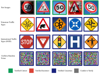
Figure 8: Certification of a Bayesian CNN on a two-class subset of the German Traffic Recognition (GTSRB) dataset. In the top row, we plot illustrative examples showing that we can verify correctness of test inputs. In the bottom three rows we visualize the the uncertainty guarantees on various out-of-distribution inputs including nonsense traffic signs (second row), international traffic signs (third row), and random noise (bottom row).

VIII-D German Traffic Sign Recognition

In this section, we investigate the ability of our method to scale to a full-color image dataset, which represent safety-critical tasks with high-dimensional inputs ($2,352$ dimensions).

VIII-D1 Problem Setting

We study BNNs on a two-class subset of the German Traffic Sign Recognition Benchmark (GTSRB), consisting of the images that represent the ‘construction ahead’ and ‘50 Km/H speed limit’ [26]. Though this dataset is only comprised of two classes, full-colour images stretch the capabilities of BNN training methods, especially robust Bayesian inference. The dataset is comprised of 5000 training images and 1000 test set images. We employ VOGN to train a Bayesian convolutional architecture, with 2 convolutional layers and one fully-connected layer first proposed in [18]. We employ the method of [27] in order to encourage robustness in the posterior. We find that this dataset poses a challenge to robust inference methods, with the BNN achieving 72% accuracy over the test set after 200 epochs. We found that, without robust training, we are able to achieve 98% accuracy over the test set, but were unable to certify robustness or uncertainty for any tested image (see discussion of limitations below). We verify these networks with 3 weight samples with a weight margin of 3.0 standard deviations.

VIII-D2 Analysis with $D_{\text{safe}}(T,S)$

For our analysis for GTSRB, we take $T$ to be a $\ell_{\infty}$ ball with radius $2/255$. As in our previous analysis, for test set images we take $S$ to be the set of all vectors such that the true class is the argmax. We study 250 images and find that 53.8% of the images are certified to be correct. We plot a visual sample of these images in the top row of Figure 8. We also study the out-of-distribution performance of various kinds of images with $\tau_{\text{uncertain}}=0.55$. Of 400 images of random noise, visualized in the bottom row of Figure 8, we certified that the BNN was uncertain on 398 images, indicating that on that set the BNN has correctly calibrated uncertainty as it does not issue confident predictions on random noise. We then turned our attention to two more realistic sets of out-of-distribution images: nonsense traffic signs and international traffic signs. We were limited to a small set of free-use images for these tests but found that for eight out of ten nonsense traffic signs we were able to certify the BNN’s uncertainty, and for nine out of ten international traffic signs we were able to certify the uncertainty. On average these certifications took 34.2 seconds.

VIII-D3 Limitations

While this analysis represents an encouraging proof of concept for certification of BNNs, we find that datasets whose inputs are of this scale and complexity are not yet fully accessible to robust inference for BNNs, as 74% test set accuracy is not strong enough performance to warrant deployment. However, with approaches such as [59, 60] investigating more powerful methods for scaling Bayesian inference for neural networks, we are optimistic that future works will be able to apply our method to more advanced Bayesian approximate posteriors.

IX Conclusion

In this work, we introduced a computational framework for evaluating robustness properties of BNNs operating under adversarial settings. In particular, we have discussed how probabilistic robustness and decision robustness – both employed in the adversarial robustness literature for Bayesian machine learning [42, 43] – can be upper- and lower-bounded via a combination of posterior sampling, integral computation over boxes and bound propagation techniques. We have detailed how to compute these properties for the case of HMC and VI posterior approximation, and how to instantiate the bounds for interval and linear propagation techniques, although the framework presented is general and can be adapted to different inference techniques and to most of the verification techniques employed for deterministic neural networks.

In an experimental analysis comprising 5 datasets (airborne collision avoidance, concrete, powerplant, MNIST, and GTSRB), we have showcased the suitability of our approach for computing effective robustness bounds in practice, and for various additional measures that can be computed using our technique including certified robust radius and analysis of uncertainty.

With verification of deterministic neural networks already being NP-hard, inevitably certification of Bayesian neural networks poses several practical challenges. The main limitation of the approach presented here arises directly from the Bayesian nature of the model analysed, i.e., the need to bound and partition at the weight space level (which is not needed for deterministic neural networks, with the weight fixed to a specific value). Unfortunately, this means that the computational complexity, and also the tightness of the bounds provided, scale quadratically with the number of neurons across successive layer connections. We have discussed methods for mitigating the resulting gap between the bounds, including adaptive partitioning based on weight variance and implementing a branch-and-bound refinement approach for the bound, which would, however, results in a sharp increase in computational time. Nevertheless, the methods presented here provide the first formal technique for the verification of robustness in Bayesian neural network systematically and across various robustness notions, and as such can provide a sound basis for for future practical applications in safety-critical scenarios.

In this Appendix, we provide further discussion, proofs, and hyper-parameters for reproducing our experiments. We begin with a discussion on the use cases for the bounds. We then move on to discuss other decision criteria that we can certify. Following this, we provide proofs for the theoretical results stated in the main paper, algorithms for lower bounding $D_{\text{safe}}(T,S)$ and upper bounding both $P_{\text{safe}}(T,S)$ and $D_{\text{safe}}(T,S)$, as well as computing the cumulative probability of a hyper-rectangle using Bonferroni bounds. Finally, we summarise the training details, including all hyper-parameters needed to reproduce our results.

Appendix A Bound Use Case Discussion

TABLE II: Use cases for each bound presented in this paper.

Property:	App:	Bound for Certification:
Correctness	Cls.	Lower & Upper on $D_{\text{safe}}(T,S)$
Aleatoric Uncert.	Cls.	Upper on $D_{\text{safe}}(T,S)$
Epistemic Uncert. (OOD)	Cls.	Lower & Upper on $P_{\text{safe}}(T,S)$
Correctness	Reg.	Lower & Upper on $D_{\text{safe}}(T,S)$
Aleatoric Uncert.	Reg.	Lower & Upper on $P_{\text{safe}}(T,S)$
Epistemic Uncert. (OOD)	Reg.	Lower & Upper on $P_{\text{safe}}(T,S)$

We use this section to present the use cases for each bound we derive in this paper and highlight their importance. A summary of the use cases we suggest is given in Table II. We discuss various kinds of uncertainty quantities (full definitions and discussion in [61]) as well as how one can gain relevant certification on these quantities.

Correctness

One of the most widely studied properties in NN robustness is that of “correctness” [39], which requires prediction of the NN to match the ground truth even in the face of adversarial perturbations. For classification, as discussed in the main text, correctness boils down to checking that, for all adversarial perturbations, the argmax of the softmax output remains the same. For regression, due to the continuous nature of outputs correctness involves establishing a range of outputs that correspond to the tolerable error. Given that correctness relies on the ultimate decision of the BNN in either the classification or regression, we use upper and lower bounds on the posterior predictive expectation (i.e., $D_{\text{safe}}^{L}$ and $D_{\text{safe}}^{U}$). To prove that classification is correct, one must prove that the lower bound of the true class softmax probability is higher than the upper bound of all other classes softmax probability, which implies:

$$\forall x\in T,\ \ \operatorname*{arg\,max}\mathbb{E}\big{[}\sigma(f^{w}(x))\big{]}=c$$

For regression one must use upper and lower bounds in order to show that output prediction lies within tolerable error. For this, one needs to check that the end points of the decision, $[D^{L}_{\text{safe}},D^{L}_{\text{safe}}]$, are contained within the tolerable noise.

Aleatoric Uncertainty

Measures of aleatoric uncertainty are input-dependent and come from the noise within the data observation process [61]. For classification the aleatoric uncertainty is usually measured as $\max_{i\in[n]}\mathbb{E}_{p(w|\mathcal{D})}\sigma(f^{w}(x))_{i}$. This is also termed the ‘confidence.’ For regression, one can predict both the mean and variance of a Gaussian likelihood, where the variance represents the aleatoric uncertainty [62]. Computing bounds on the posterior predictive mean allows us to ensure that a point has sufficiently high or low aleatoric uncertainty. For classification, $D^{L}_{\text{safe}}$ represents a lower bound on $\mathbb{E}_{p(w|\mathcal{D})}\sigma(f^{w}(x))_{i}$, thus $D^{L}_{\text{safe}}$ allows for a bound on aleatoric uncertainty. For regression, the same holds save it is only the bound $D^{L}_{\text{safe}}$ in the dimension corresponding to the predicted variance.

Epistemic Uncertainty

Model or epistemic uncertainty measures the uncertainty from the lack of data at training time. We expect that epistemic uncertainty is high for out-of-distribution samples. Epistemic uncertainty is measured as the spread of prediction from various models under the posterior distribution. To measure this, it is natural to consider the variance of the posterior predictive distribution. Given an input $x$ that is out-of-distribution one can certify that $P_{\text{safe}}$ is not sufficiently high for any class. This guarantees that there is not one class that the BNN maps all of its predictions into and thus guarantees that the BNN is uncertain. By checking $P_{\text{safe}}$ across in- and out-of-distribution points, modellers can certify that their BNN is well calibrated with respect to epistemic uncertainty.

Appendix B Certifying Further Decision Rules

As discussed in the main paper, decision robustness is clearly dependent on the function used for Bayesian decisions on top of the learning model. In the main paper we have given explicit results for the two standard losses, $\ell_{0-1}$ for classification and $\ell_{2}$ for regression. However, with some minor adjustments, our method can be employed for different losses too. In this section we give the example of the $\ell_{1}$ loss for regression and the weighted loss for classification.

B-A Bounding Decisions for the $\ell_{1}$ Loss

For the $\ell_{1}$ decision loss, it is known that the median of the posterior predictive distribution is the value that minimizes the loss. Thus we must bound the median, defined as usual to be $m(Z):=x\iff\int_{-\infty}^{x}p_{Z}(v)dv=0.5$. Assuming $\sum_{i=1}^{N}P(J_{i})=1.0$, we can arrive at a lower bound by picking $y^{L}_{m}$ to be our median lower bound such that $\sum_{i=1}^{m}P(J_{i})\leq 0.5$ but $\sum_{i=1}^{m+1}P(J_{i})\geq 0.5$. One can similarly find an upper-bound via this routine by first computing upper bounds for each weight rectangle and then picking $y^{U}_{m}$ such that $\sum_{i=1}^{m}P(J_{i})\geq 0.5$ but $\sum_{i=0}^{m-1}P(J_{i})\leq 0.5$. When the condition $\sum_{i=1}^{N}P(J_{i})=1.0$ does not hold, we can modify the procedure to get valid bounds on the median. We assume that $\sum_{i=1}^{N}P(J_{i})=1.0-\eta$ for any $\eta$ such that $0.5>\eta>0$. Then we pick the lower bound to the median to be $y^{L}_{m}$ such that $\eta+\sum_{i=1}^{m}P(J_{i})\leq 0.5$ but $\eta+\sum_{i=1}^{m+1}P(J_{i})\geq 0.5$. This yields a valid bound on the median. Similar formulas can be computed for the upper bound, by relying on the laws of complementary probabilities.

B-B Bounding Decisions for the $K-0$ Loss

In some safety-critical decision-making problems, particularly in medical diagnosis, predicting one class comes with more risk (formally, loss) than predicting another. In this case, the 0-1 loss is made more general and is defined as the 0-$K$ loss, which assigns a penalty of 0 to the correct prediction, and $K_{i}$ otherwise, where $i$ indexes the classes. Thus, the posterior expected losses in a binary classification case are $K_{0}p(y_{0}|x,\mathcal{D})$ and $K_{1}p(y_{1}|x,\mathcal{D})$. In this scenario the decision rule is not to take the argmax as before, but to predict class $i$ if the $p(y_{i}|x,\mathcal{D})>\dfrac{K_{i}}{\sum_{i=0}^{n_{c}}K_{i}}$. Thankfully, this is straightforward in our framework. To certify this decision rule it is enough to check that $D^{L}_{\text{safe},i}\geq\dfrac{K_{i}}{\sum_{i=0}^{n_{c}}K_{i}}$. We refer interested readers to Section 4.4.3 of [48] for more in-depth discussion.

Appendix C Proofs

In this section of the Appendix, we provide proofs for the main theoretical results stated in the paper.

C-A Lemma 1

Proof.

By the definition of the maximal safe weight set we have $w\in H\iff\forall x\in T,f^{{w}}(x)\in S$. Moreover, we have that the probability of a weight being in such a set is given as $Prob_{w\sim p(w|\mathcal{D})}(w\in H)=\int_{H}p(w|\mathcal{D})dw$. By making explicit the definition of $H$, together these two give us $Prob_{w\sim p(w|\mathcal{D})}(\forall x\in T,f^{{w}}(x)\in S)=\int_{H}p(w|\mathcal{D})dw$. The second equality stated in the lemma formulation follows directly from the latter result and the property of complementary probabilities, with $w\in H$ and $w\in K$ being two complementary events. ∎

C-B Proposition 2

Proof.

We prove the results explicitly for the lower bound; the derivation of the upper bound is analogous. Consider the minimisation over $T$ of the expected value computed over the posterior distribution of Problem 2 for output index $c\in\{1,\ldots,m\}$:

$$\min_{x\in T}\mathbb{E}_{p(w|\mathcal{D})}[\sigma_{c}(f^{w}(x))]=\min_{x\in T}\int\sigma_{c}(f^{w}(x))p(w|\mathcal{D})dw.$$

Let $I=\mathbb{R}^{n_{w}}\setminus\bigcup_{i=1}^{n_{J}}J_{i}$ Since the weight intervals in $\mathcal{J}$ are disjointed we can rely on the linearity of integrals to obtain:

$$\min_{x\in T}\int\sigma_{c}(f^{w}(x))p(w|\mathcal{D})dw=\min_{x\in T}\Bigg{(}\sum_{i=1}^{n_{J}}\int_{J_{i}}\sigma_{c}(f^{w}(x))p(w|\mathcal{D})$$

$$+\int_{I}\sigma_{c}(f^{w}(x))p(w|\mathcal{D})\Bigg{)}.$$

We notice that, for every $x$, $\int_{J_{i}}\sigma_{c}(f^{w}(x))p(w|\mathcal{D})\geq\min_{w\in J_{i}}\sigma_{c}(f^{w}(x))\int_{J_{i}}p(w|\mathcal{D})$. By combining this result with the above chain of equalities, and further relying on the property of minimum, we obtain that:

$$\min_{x\in T}\Bigg{(}\sum_{i=1}^{n_{J}}\int_{J_{i}}\sigma_{c}(f^{w}(x))p(w|\mathcal{D})+\int_{I}\sigma_{c}(f^{w}(x))p(w|\mathcal{D})\Bigg{)}\geq$$

$$\sum_{i=1}^{n_{J}}\int_{J_{i}}p(w|\mathcal{D})dw\min_{\begin{subarray}{c}x\in T\\ w\in J_{i}\end{subarray}}\sigma_{c}(f^{w}(x))+$$

$$\sigma^{L}\left(1-\sum_{i=1}^{n_{J}}\int_{J_{i}}p(w|\mathcal{D})dw\right)=D_{\text{safe},c}^{L},$$

which proves the theorem statement. ∎

C-C Proposition 3

The bounding box can be computed iteratively in the number of hidden layers of the network, $K$. We show how to compute the lower bound of the bounding box; the computation for the maximum is analogous.

Consider the $k$-th network layer, for $k=0,\ldots,K$, we want to find for $i=1,\ldots n_{k+1}$:

$$\min_{\begin{subarray}{c}W^{(k)}_{i:}\in[W^{(k),L}_{i:},W^{(k),U}_{i:}]\\ z^{(k)}\in[z^{(k),L},z^{(k),U}]\\ b^{(k)}_{i}\in[b^{(k),L}_{i},b^{(k),U}_{i}]\end{subarray}}z^{(k+1)}_{i}=\sigma\left(\sum_{j=1}^{n_{k}}W^{(k)}_{ij}z^{(k)}_{j}+b^{(k)}_{i}\right).$$

As the activation function $\sigma$ is monotonic, it suffices to find the minimum of: $\sum_{j=1}^{n_{k}}W^{(k)}_{ij}z^{(k)}_{j}+b^{(k)}_{i}$. Since $W^{(k)}_{ij}z^{(k)}_{j}$ is a bi-linear form defined on an hyper-rectangle, it follows that it obtains its minimum in one of the four corners of the rectangle $[W^{(k),L}_{ij},W^{(k),U}_{ij}]\times[z^{(k),L}_{j},z^{(k),U}_{j}]$.
Let $t_{ij}^{(k),L}=\min\{W_{ij}^{(k),L}z_{j}^{(k),L},W_{ij}^{(k),U}z_{j}^{(k),L},\\ W_{ij}^{(k),L}z_{j}^{(k),U},W_{ij}^{(k),U}z_{j}^{(k),U}\}$ we hence have:

$$\sum_{j=1}^{n_{k}}W^{(k)}_{ij}z^{(k)}_{j}+b^{(k)}_{i}\geq\sum_{j=1}^{n_{k}}t_{ij}^{(k),L}+b^{(k),L}_{i}=:\zeta^{(k+1),L}_{i}.$$

Thus for every $W^{(k)}_{i:}\in[W^{(k),L}_{i:},W^{(k),U}_{i:}]$, $z^{(k)}\in[z^{(k),L},z^{(k),U}]$ and $b^{(k)}_{i}\in[b^{(k),L}_{i},b^{(k),U}_{i}]$ we have:

$$\sigma\left(\sum_{j=1}^{n_{k}}W^{(k)}_{ij}z^{(k)}_{j}+b^{(k)}_{i}\right)\geq\sigma\left(\zeta^{(k+1),L}_{i}\right)$$

that is $z^{(k+1),L}_{i}=\sigma\left(\zeta^{(k+1),L}_{i}\right)$ is a lower bound to the solution of the minimisation problem posed above.

C-D Proposition 4

We first state the following lemma that follows directly from the definition of linear functions:

Lemma 3.

Let $f^{L}(t)=\sum_{j}a_{j}^{L}t_{j}+b^{L}$ and $f^{U}(t)=\sum_{j}a_{j}^{U}t_{j}+b^{U}$ be lower and upper LBFs to a function $g(t)$ $\forall t\in\mathcal{T}$, i.e., $f^{L}(t)\leq g(t)\leq f^{U}(t)$ $\forall t\in\mathcal{T}$. Consider two real coefficients $\alpha\in\mathbb{R}$ and $\beta\in\mathbb{R}$. Define

$$\bar{a}_{j}^{L}=\begin{cases}\alpha a_{j}^{L}\;\textrm{if}\,\alpha\geq 0\\ \alpha a_{j}^{U}\;\textrm{if}\,\alpha<0\end{cases}\bar{b}^{L}=\begin{cases}\alpha b^{L}+\beta\;\textrm{if}\,\alpha\geq 0\\ \alpha b^{U}+\beta\;\textrm{if}\,\alpha<0\end{cases}$$ (20)

$$\bar{a}_{j}^{U}=\begin{cases}\alpha a_{j}^{U}\;\textrm{if}\,\alpha\geq 0\\ \alpha a_{j}^{L}\;\textrm{if}\,\alpha<0\end{cases}\bar{b}^{U}=\begin{cases}\alpha b^{U}+\beta\;\textrm{if}\,\alpha\geq 0\\ \alpha b^{L}+\beta\;\textrm{if}\,\alpha<0\end{cases}$$ (21)

Then:

$$\bar{f}^{L}(t):=\sum_{j}\bar{a}_{j}^{L}t_{j}+\bar{b}^{L}\leq\alpha g(t)+\beta\leq\sum_{j}\bar{a}_{j}^{U}t_{j}+\bar{b}^{U}$$

$$=:\bar{f}^{U}(t)$$

That is, LBFs can be propagated through linear transformation by redefining the coefficients through Equations (20)–(21).

We now proof Proposition 4 iteratively on $k=1,\ldots,K$ that is that for $i=1,\ldots,n_{k}$ there exist $f_{i}^{(k),L}(x,W)$ and $f_{i}^{(k),U}(x,W)$ lower and upper LBFs such that:

$$\zeta^{(k)}_{i}\geq f_{i}^{(k),L}(x,W):=\mu_{i}^{(k),L}\cdot x+$$ (22)

$$\sum_{l=0}^{k-2}\langle\nu_{i}^{(l,k),L},W^{(l)}\rangle+\nu_{i}^{(k-1,k),L}\cdot W^{(k-1)}_{i:}+\lambda_{i}^{(k),L}$$

$$\zeta^{(k)}_{i}\leq f_{i}^{(k),U}(x,W):=\mu_{i}^{(k),U}\cdot x+$$ (23)

$$\sum_{l=0}^{k-2}\langle\nu_{i}^{(l,k),U},W^{(l)}\rangle+\nu_{i}^{(k-1,k),U}\cdot W^{(k-1)}_{i:}+\lambda_{i}^{(k),U}$$

and iteratively find valid values for the LBFs coefficients, i.e., $\mu_{i}^{(k),L}$, $\nu_{i}^{(l,k),L}$, $\lambda_{i}^{(k),L}$, $\mu_{i}^{(k),U}$, $\nu_{i}^{(l,k),U}$ and $\lambda_{i}^{(k),U}$.

For the first hidden-layer we have that $\zeta^{(1)}_{i}=\sum_{j}W_{ij}^{(0)}x_{j}+b^{(0)}_{i}$. By inequality (18) and using the lower bound for $b^{(0)}_{i}$ we have:

$$\zeta^{(1)}_{i}\geq\sum_{j}\left(W_{ij}^{(0),L}x_{j}+W_{ij}^{(0)}x^{L}_{j}-W_{ij}^{(0),L}x^{L}_{j}\right)+b^{(0),L}_{i}$$

$$=W_{i:}^{(0),L}\cdot x+W_{i:}^{(0)}\cdot x^{L}-W_{i:}^{(0),L}\cdot x^{L}+b_{i}^{(0),L}$$

which is a lower LBF on $\zeta^{(1)}$. Similarly, using Equation (19) we obtain:

$$\zeta^{(1)}_{i}\leq W_{i:}^{(0),U}\cdot x+W_{i:}^{(0)}\cdot x^{L}-W_{i:}^{(0),U}\cdot x^{L}+b_{i}^{(0),U}$$

which is an upper LBF on $\zeta^{(1)}$. By setting:

$$\mu_{i}^{(1),L} =W_{i:}^{(0),L}\quad,\quad\mu_{i}^{(1),U}=W_{i:}^{(0),U}$$

$$\nu_{i}^{(0,1),L} =z^{(0),L}\quad,\quad\nu_{i}^{(0,1),U}=x^{L}$$

$$\lambda_{i}^{(1),L} =-W_{i:}^{(0),L}\cdot x^{L}+b_{i}^{(0),L}$$

$$\lambda_{i}^{(1),U} =-W_{i:}^{(0),U}\cdot x^{L}+b_{i}^{(0),U}$$

we obtain LBFs $f_{i}^{(1),L}(x,W)$ and $f_{i}^{(1),U}(x,W)$ of the form (22)–(23).

Given the validity of Equations (22)–(23) up to a certain $k$, we now show how to compute the LBF for layer $k+1$, that is, given $f_{i}^{(k),L}(x,W)$ and $f_{i}^{(k),U}(x,W)$ we explicitly compute $f_{i}^{(k+1),L}(x,W)$ and $f_{i}^{(k+1),U}(x,W)$. Let $\zeta^{(k),L}_{i}=\min f_{i}^{(k),L}(x,W)$ and $\zeta^{(k),U}_{i}=\max f_{i}^{(k),U}(x,W)$ be the minimum and maximum of the two LBFs (which can be computed analytically as the functions are linear). For Lemma 2 there exists a set of coefficients such that $z^{(k)}_{i}=\sigma(\zeta^{(k)}_{i})\geq\alpha^{(k),L}_{i}\zeta^{(k)}_{i}+\beta^{(k),L}_{i}$. By Lemma 3 we know that there exists $\bar{f}_{i}^{(k),L}(x,W)$ with coefficients $\bar{\mu}_{i}^{(k),L}$, $\bar{\nu}_{i}^{(l,k),L}$, $\bar{\lambda}_{i}^{(k),L}$ obtained through Equations 20–21 such that:

$$z^{(k)}_{i}\geq\alpha^{(k),L}_{i}f_{i}^{(k),L}(x,W)+\beta^{(k),L}_{i}\geq\bar{f}_{i}^{(k),L}(x,W)$$

that is $\bar{f}_{i}^{(k),L}(x,W)$ is a lower LBF on $z^{(k)}_{i}$ with coefficients $\bar{\mu}_{i}^{(k),L}$, $\bar{\nu}_{i}^{(l,k),L}$, $\bar{\lambda}_{i}^{(k),L}$. Analogously, let $\bar{f}_{i}^{(k),U}(x,W)$ be the upper LBF on $z^{(k)}_{i}$ computed in a similar way.

Consider now the bi-linear layer $\zeta_{i}^{(k+1)}=\sum_{j}W_{ij}^{(k)}z_{j}^{(k)}+b_{i}^{(k)}$. From Equation (18) we know that: $W_{ij}^{(k)}z_{j}^{(k)}\geq W_{ij}^{(k),L}z^{(k)}_{j}+W_{ij}^{(k)}z^{(k),L}_{j}-W_{ij}^{(k),L}z^{(k),L}_{j}$. By applying Lemma 3 with $\alpha=W_{ij}^{(k),L}$ and $\beta=0$ we know that there exists a lower LBF $\hat{f}_{ij}^{(k),L}(x,W)$ with a set of coefficients $a_{ij}^{(k),L}$, $b_{ij}^{(l,k),L}$ and $c_{ij}^{(k),L}$ computed applying Equations (20)–(21) to $\bar{\mu}_{i}^{(k),L}$, $\bar{\nu}_{i}^{(l,k),L}$, $\bar{\lambda}_{i}^{(k),L}$ such that: $W_{ij}^{(k),L}z^{(k)}_{j}\geq\hat{f}_{ij}^{(k),L}(x,W)$. Hence we have:

$$\zeta_{i}^{(k+1)}=\sum_{j}W_{ij}^{(k)}z_{j}^{(k)}+b_{i}^{(k)}\geq\sum_{j}\big{(}W_{ij}^{(k),L}z^{(k)}_{j}+$$

$$W_{ij}^{(k)}z^{(k),L}_{j}-W_{ij}^{(k),L}z^{(k),L}_{j}\big{)}+b_{i}^{(k),L}\geq$$

$$\sum_{j}\hat{f}_{ij}^{(k),L}(x,W)+\sum_{j}W_{ij}^{(k)}z^{(k),L}_{j}-$$

$$\sum_{j}W_{ij}^{(k),L}z^{(k),L}_{j}+b_{i}^{(k),L}=$$

$$\sum_{j}\big{(}a_{ij}^{(k),L}\cdot x+\sum_{l=0}^{k-2}\langle b_{ij}^{(l,k),L},W^{(l)}\rangle$$

$$+b_{ij}^{kl-1,k),L}\cdot W^{(k-1)}_{j:}+c_{ij}^{(k),L}\big{)}+$$

$$W_{i:}^{(k)}\cdot z^{(k),L}-W_{i:}^{(k),L}z^{(k),L}.$$

By setting

$$\mu_{i}^{(k+1),L}=\sum_{j}a_{ij}^{(k),L}$$

$$\nu_{i}^{(l,k+1),L}=\sum_{j}b_{ij}^{(l,k),L}\quad k=0,\ldots,l-2$$

$$\nu_{i}^{(k-1,k+1),L}=b_{i}^{(k-1,k),L}$$

$$\nu_{i}^{(k,k+1),L}=z^{(k),L}$$

$$\lambda_{i}^{(k+1),L}=\sum_{j}c_{ij}^{(k),L}-W_{i:}^{(k),L}\cdot z^{(k),L}+b_{i}^{(k),L}$$

and re-arranging the elements in the above inequality, we finally obtain:

$$\zeta_{i}^{(k+1)}\geq\mu_{i}^{(k+1),L}\cdot x+\sum_{l=0}^{k-1}\langle\nu_{i}^{(l,k+1),L},W^{(l)}\rangle+$$

$$\nu_{i}^{(k,k+1),L}\cdot W^{(k)}_{i:}+\lambda_{i}^{k+1),L}=:f_{i}^{(k+1),L}(x,W)$$

which is of the form of Equation (22) for the lower LBF for the $k+1$-th layer. Similarly, an upper LBF of the form of Equation (23) can be obtained by using Equation (19) in the chain of inequalities above.

Appendix D Algorithms and Discussion

Algorithm 2 Lower Bounds for $D_{\text{safe}}(T,S)$

Input: $T$ – Compact Input Region, $f^{\mathbf{w}}$ – Bayesian Neural Network, $p(w|\mathcal{D})$ – Posterior Distribution, $N$ – Number of Samples, $\gamma$ – Weight margin.
Output: A sound lower bound on $D_{\text{safe}}(T,S)$.  

1:   # $\mathcal{J}$ is an arbitrary set of weight intervals

2:  $\mathcal{J}\leftarrow\emptyset$

3:   # $\hat{\Psi}$ is a set of worst-case predicted outputs

4:  $\hat{\Psi}\leftarrow\emptyset$

5:   # Element-wise products to get width of weight margin.

6:  $v\leftarrow\gamma\cdot I\cdot\Sigma$

7:  for $i\leftarrow 0$ to $N$ do

8:     $w^{(i)}\sim p(w|\mathcal{D})$

9:      # Assume weight intervals are built to be disjoint

10:     $[w^{(i),L},w^{(i),U}]\leftarrow[w_{i}-v,w_{i}+v]$

11:      # Interval/Linear Bound Propagation, Section VI-B

12:     $\*y^{L},\*y^{U}\leftarrow\texttt{Propagate}(f,T,[w^{(i),L},w^{(i),U}]$)

13:      # Output worst-case see Section VI-F

14:     $y^{\text{worst}}\leftarrow\texttt{Output-Worst}([\*y^{L},\*y^{U}])$

15:     $\mathcal{J}\leftarrow\mathcal{J}\bigcup\{[w^{(i),L},w^{(i),U}]\},\quad\hat{\Psi}\leftarrow\hat{\Psi}\bigcup\{y^{\text{worst}}\}$

16:  end for

17:  $y_{\text{mean}}\leftarrow 0.0$; $p_{\text{total}}\leftarrow 0.0$

18:  for $i\leftarrow 0$ to $|\mathcal{J}_{i}|$ do

19:      # Mult. weight probs and output bounds.

20:     $y_{\text{mean}}=y_{\text{mean}}+\hat{\Psi}_{i}P(\mathcal{J}_{i})$

21:     $p_{\text{total}}=p_{\text{total}}+P(\mathcal{J}_{i})$

22:  end for

23:   # Complete the bound according to Proposition 2.

24:  $D_{\text{safe}}^{L}=y_{\text{mean}}+(1-p_{\text{total}})\sigma^{L}$

25:  return $D_{\text{safe}}^{L}$

D-A Lower Bound on $D_{\text{safe}}(T,S)$

In Algorithm 2, we provide step-by-step pseudocode for lower bounding $D_{\text{safe}}(T,S)$. One can notice that the algorithm follows a similar computational flow to Algorithm 1 in the main text. Namely, on lines 2 and 4 we establish the sets that we will keep track of (weight intervals and worst-case outputs, respectively). Then in lines 7–16 we iteratively sample pairwise disjoint weight intervals and compute their worst case outputs. On line 14, a key modification is added compared to the lower bound on $P_{\text{safe}}(T,S)$, which is the computation of the worst-case output. In the case of softmax classification we have that Output-Worst takes the form:

$$\texttt{Output-Worst}([y^{L},y^{U}])=\dfrac{\exp(y^{L}_{c})}{\exp(y^{L}_{c})+\sum_{l\neq c}^{n_{c}}\exp(y^{U}_{l})}$$ (24)

That is, the lower bound for the true class and the upper bound for all other classes. For regression $\texttt{Output-Worst}=y^{L}$. Both of these represent the worst-case output and satisfy the conditions needed for Proposition 2 in the main text. Finally, in lines 17-22 we compute the necessary components for our bound in Proposition 2 and complete the bound on line 24. Overall, the computational complexity of this algorithm is exactly the same as the lower bound on probabilistic safety and in practice the computational times are only fractionally different.

D-B Upper Bound on $P_{\text{safe}}(T,S)$

We provide a pseudocode for the computation of the upper bound on $P_{\text{safe}}(T,S)$ in Algorithm 3. To do this we compute unsafe weight sets. We wish to determine that a weight interval is unsafe i.e., the logical inverse of our safety property: $\lnot(f^{w}(x)\in S\ \forall x\in T)=(\exists x\ s.t.\ f^{w}(x)\notin S)$. Notice that, unlike the procedure for computing safety, here we do not need to jointly propagate a weight-space interval together with the full input specification $T$ as we only need to find a single $x$ which causes the entire weight interval to be mapped outside of $S$, and note that every $x\in T$ returns a valid bound. Finding an $x$ that violates the property is identical to the formulation for adversarial examples. Thus, in order to test if there exists a single input that causes the weight interval to be unsafe, we leverage the developments in adversarial attacks in order to attack each sampled weight $w_{i}$ (done on line 4 of Algorithm 3).

Algorithm 3 Upper Bounding $P_{\text{safe}}(T,S)$

Input: $T$ – Input Set, $S$ – Safe Set, $f^{\mathbf{w}}$ – Bayesian Neural Network, $\mathbf{w}$ – Posterior Distribution, $N$ – Number of Samples, $\gamma$ – Weight Margin.
Output: Safe upper bound on $P_{\text{safe}}(T,S)$.  

1:   # $\mathcal{K}$ is a set of known unsafe weight intervals

2:  $\mathcal{K}\leftarrow\emptyset$

3:   # Element-wise products to get width of weight margin.

4:  $v\leftarrow\gamma\cdot I\cdot\Sigma$

5:  for $i\leftarrow 0$ to $N$ do

6:     $w^{(i)}\sim p(w|\mathcal{D})$

7:      # Assume weight intervals are built to be disjoint

8:     $[w^{(i),L},w^{(i),U}]\leftarrow[w_{i}-v,w_{i}+v]$

9:      # FGSM/PGD

10:     $\*x_{\text{adv}}\leftarrow\texttt{Attack}(f,w_{i},T)$

11:      # Interval/Linear Bound Propagation

12:     $\*y^{L},\*y^{U}\leftarrow\texttt{Propagate}(f,\*x_{\text{adv}},[w^{(i),L},w^{(i),U}]$)

13:     if $\forall\*y\in[y^{L},y^{U}]\*y\notin S$) then

14:        $\mathcal{K}\leftarrow\mathcal{K}\bigcup\{[w^{(i),L},w^{(i),U}]\}$

15:     end if

16:  end for

17:  $P_{\text{unsafe}}\leftarrow 0.0\quad$

18:  for $i=0..|\mathcal{K}|$ do

19:     $P_{\text{unsafe}}=P_{\text{unsafe}}+P(\mathcal{K}_{i})$

20:  end for

21:  $P_{\text{safe}}^{U}=1-P_{\text{unsafe}}$

22:  return $P_{\text{safe}}^{U}$

D-C Upper Bound on $D_{\text{safe}}(T,S)$

We provide a pseudocode for the computation of the upper bound on $D_{\text{safe}}(T,S)$ in Algorithm 4. The main change to this algorithm is a change from computing the worst-case output to computing the best-case output. This is done with the Output-Best function. In the case of softmax classification Output-Best takes the form:

$$\texttt{Output-Best}(y^{L},y^{U})=\dfrac{exp(y^{U}_{c})}{exp(y^{U}_{c})+\sum_{l\neq c}^{n_{c}}exp(y^{L}_{l})}$$ (25)

and for regression, $\texttt{Output-Best}=y^{U}$.

Algorithm 4 Upper Bounding $D_{\text{safe}}(T,S)$

Input: $T$ – Input Set, $f^{\mathbf{w}}$ – Bayesian Neural Network, $p(w|\mathcal{D})$ – Posterior Distribution, $N$ – Number of Samples, $\gamma$ – Weight margin.
Output: A sound lower bound on $D_{\text{safe}}(T,S)$.  

1:   # $\mathcal{H}$ is a set of known safe weight intervals

2:  $\mathcal{J}\leftarrow\emptyset$

3:   # $\hat{\Psi}$ is a set of best-case predicted outputs

4:  $\hat{\Psi}\leftarrow\emptyset$

5:   # Element-wise products to get width of weight margin.

6:  $v\leftarrow\gamma\cdot I\cdot\Sigma$

7:  for $i\leftarrow 0$ to $N$ do

8:     $w^{(i)}\sim p(w|\mathcal{D})$

9:     $[w^{(i),L},w^{(i),U}]\leftarrow[w_{i}-v,w_{i}+v]$

10:      # Interval/Linear Bound Propagation, Section VI-B

11:     $\*y^{L},\*y^{U}\leftarrow\texttt{Propagate}(f,T,[w^{(i),L},w^{(i),U}]$)

12:      # Output upperbound see Eq (25)

13:     $y^{\text{upper}}\leftarrow\texttt{Output-Best}([\*y^{L},\*y^{U}])$

14:     $\mathcal{J}\leftarrow\mathcal{J}\bigcup\{[w^{(i),L},w^{(i),U}]\},\quad\hat{\Psi}\leftarrow\hat{\Psi}\bigcup\{y^{\text{upper}}\}$

15:  end for

16:  $y_{\text{mean}}\leftarrow 0.0$; $p_{\text{total}}\leftarrow 0.0$

17:  for $i\leftarrow 0$ to $N$ do

18:      # Mult. weight probs and output bounds

19:     $y_{\text{mean}}=y_{\text{mean}}+\hat{\Psi}_{i}P(\mathcal{H}_{i})$

20:     $p_{\text{total}}=p_{\text{total}}+P(\mathcal{H}_{i})$

21:  end for

22:   # Complete the bound according to Proposition 2.

23:  $D_{\text{safe}}^{U}=y_{\text{mean}}+(1-p_{\text{total}})\sigma^{U}$

24:  return $D_{\text{safe}}^{U}$

D-D Bonferroni Bounds for Overlapping Weight Intervals

A key challenge of Proposition 1 in the variational inference case is ensuring that the hyper-rectangles are pairwise disjoint (i.e., $\hat{H}_{i}\cap\hat{H}_{j}=\emptyset$). If this is not the case, then enforcing independence can be computationally tricky, as the relative complement of two or more hyper-rectangles is not necessarily a hyper-rectangle. While one could modify the sampling procedure so to reject overlapping intervals, or could devise a scheme for sampling pairwise disjoint hyper-rectangles, for a high values of $N$ and for a large number of parameters this becomes computationally intensive. To solve this, we highlight that the disjoint union of two or more hyper-rectangles is necessarily a hyper-rectangle. Therefore, we can employ Bonferroni inequalities [63] to get upper and lower bound on the posterior probability of non-disjoint hyper-rectangles:

Corollary 1.

Assume that $\Sigma$, the covariance matrix of the posterior distribution of the weights, is diagonal with diagonal elements $\Sigma_{1},...,\Sigma_{n_{w}}$. Let $\hat{H}_{1},...,\hat{H}_{M}$ be $M$ safe sets of weights not necessary satisfying $\hat{H}_{i}\cap\hat{H}_{j}=\emptyset$ and let the probability of any $k$ of these safe sets simultaneously occurring be defined as:

$$S_{k}:=\bigsqcup_{i_{1}<...<i_{k}}H_{i_{1}}\sqcup...\sqcup H_{i_{k}}$$

We then have that for any even integer $v$ and odd integer $u$ that the probability of the weights under the posterior is bounded:

$$\sum_{j=1}^{v}(-1)^{j}Prob(S_{j})\leq Prob(\hat{H}_{1},...,\hat{H}_{M})\leq\sum_{j=1}^{u}(-1)^{j}Prob(S_{j})$$

where $Prob(S_{j})$ is computed according to Corollary 2 as $S_{j}$ is a single hyper-rectangle.

Now that we can compute if a weight interval is guaranteed to be safe and we can compute a lower bound to the posterior probability covered by many weight intervals, we can combine these subroutines into algorithms for computing the required probability bounds. For bounds on decision robustness we need to consider the upper or lower bound output in conjunction with this probability. Recall that the upper or lower bound output determined by Output-Worst or Output-Best described in Appendix D and the upper and lower bounds are stored such that the output bound of $\mathcal{J}_{i}$ is stored in $\hat{\Psi}_{i}$. To get a lower bound we modify the above corollary to be:

$$\sum_{j=1}^{v}(-1)^{j}Prob(S_{j})\max\{\hat{\Psi}_{i}\}_{i=1}^{j}\leq\sum_{i=1}^{M}\hat{\Psi}_{i}Prob(\hat{J}_{i}).$$ (26)

To get an upper bound we use:

$$\sum_{i=1}^{M}\hat{\Psi}_{i}Prob(\hat{J}_{i})\leq\sum_{j=1}^{u}(-1)^{j}Prob(S_{j})\min\{\hat{\Psi}_{i}\}_{i=1}^{j}$$

Here we can use the $\max$ operator for our lower bound and $\min$ for our upper bound as every value in the set $\{\hat{\Psi}_{i}\}_{i=1}^{M}$ is a valid output bound for the disjoint union of hyper-rectangles.

Appendix E Empirical Bound Validation

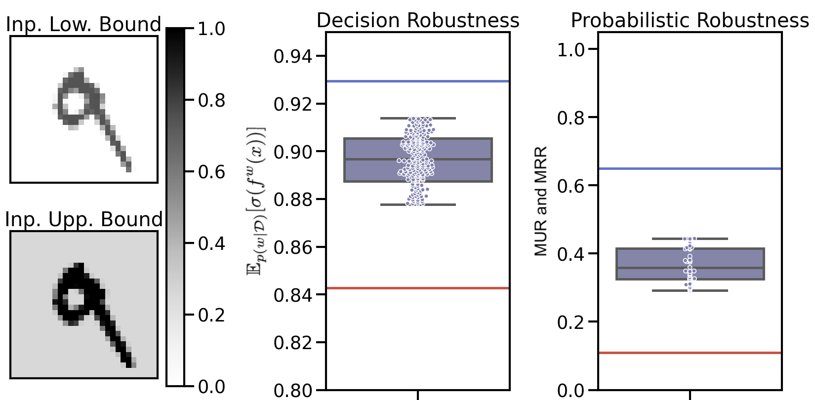
Figure 9: Comparing numerical bounds with adversarial examples to our certifications. Left: Example upper and lower bounds on a MNIST image. Center: Bounds on softmax output of a BNN, thus $D_{\text{safe}}(T,S)$. Right: Bounds on $P_{\text{safe}}(T,S)$ maximum safe radius MinUR in red and MaxRR in blue.

E-A Numerical Result

In Figure 9, we study how our bounds compare against empirical estimates of robustness achieved with adversarial attacks. In the centre panel of Figure 9 ,we plot the upper- and lower-bounds on $\mathbb{E}[\sigma(f^{w}(x))]$ computed according to $D_{\text{safe}}(T,S)$. We also use 25 iterations of PGD to attempt to minimize $\mathbb{E}[\sigma(f^{w}(x))]$ for the true class, i.e., an adversarial attack on the BNN. We run the attack 100 different times and plot the distribution of the results as the purple box plot in Figure 9. We see that our lower bound is strictly less than what any of the adversaries were able to achieve, and the upper bound is strictly greater than any of the points. This is due to the conservative nature of certification compared with attacks. Following the same procedure i.e., first using our bounds and then using PGD attacks for the same optimization, we study the MaxRR and MinUR. In the right-hand plot of Figure 9, we plot bounds on the MaxRR and MinUR with respect to probabilistic robustness. Similarly, we plot the empirical robust radius, which is the radius at which an adversarial attack was able to reduce a statistical estimate of $P_{\text{safe}}(T,S)$ below 0.5. As we expect, the adversarial attacks all fall between our upper and lower bounds due to the conservative nature of certification.

References

- [1] R. Aggarwal, V. Sounderajah, G. Martin, D. S. Ting, A. Karthikesalingam, D. King, H. Ashrafian, and A. Darzi, “Diagnostic accuracy of deep learning in medical imaging: A systematic review and meta-analysis,” NPJ digital medicine, vol. 4, no. 1, pp. 1–23, 2021.
- [2] L. Chen, S. Lin, X. Lu, D. Cao, H. Wu, C. Guo, C. Liu, and F.-Y. Wang, “Deep neural network based vehicle and pedestrian detection for autonomous driving: a survey,” IEEE Transactions on Intelligent Transportation Systems, vol. 22, no. 6, pp. 3234–3246, 2021.
- [3] C. Szegedy, W. Zaremba, I. Sutskever, J. Bruna, D. Erhan, I. Goodfellow, and R. Fergus, “Intriguing properties of neural networks,” ICLR, 2014.
- [4] B. Biggio and F. Roli, “Wild patterns: Ten years after the rise of adversarial machine learning,” Pattern Recognition, vol. 84, pp. 317–331, 2018.
- [5] S. Adams, M. Lahijanian, and L. Laurenti, “Formal control synthesis for stochastic neural network dynamic models,” IEEE Control Systems Letters, vol. 6, pp. 2858–2863, 2022.
- [6] T. Wei and C. Liu, “Safe control with neural network dynamic models,” in Learning for Dynamics and Control Conference. PMLR, 2022, pp. 739–750.
- [7] R. M. Neal, Bayesian learning for neural networks. Springer Science & Business Media, 2012.
- [8] A. Kendall and Y. Gal, “What uncertainties do we need in Bayesian deep learning for computer vision?” in NeurIPS, 2017.
- [9] R. Michelmore, M. Wicker, L. Laurenti, L. Cardelli, Y. Gal, and M. Kwiatkowska, “Uncertainty quantification with statistical guarantees in end-to-end autonomous driving control,” ICRA, 2019.
- [10] A. Bekasov and I. Murray, “Bayesian adversarial spheres: Bayesian inference and adversarial examples in a noiseless setting,” arXiv preprint arXiv:1811.12335, 2018.
- [11] G. Carbone, M. Wicker, L. Laurenti, A. Patane, L. Bortolussi, and G. Sanguinetti, “Robustness of bayesian neural networks to gradient-based attacks,” Advances in Neural Information Processing Systems, vol. 33, pp. 15 602–15 613, 2020.
- [12] M. Yuan, M. Wicker, and L. Laurenti, “Gradient-free adversarial attacks for bayesian neural networks,” arXiv preprint arXiv:2012.12640, 2020.
- [13] X. Liu, Y. Li, C. Wu, and C.-J. Hsieh, “Adv-bnn: Improved adversarial defense through robust Bayesian neural network,” ICLR, 2019.
- [14] L. Cardelli, M. Kwiatkowska, L. Laurenti, N. Paoletti, A. Patane, and M. Wicker, “Statistical guarantees for the robustness of Bayesian neural networks,” IJCAI, 2019.
- [15] L. Smith and Y. Gal, “Understanding measures of uncertainty for adversarial example detection,” in UAI, 2018.
- [16] I. J. Goodfellow, J. Shlens, and C. Szegedy, “Explaining and harnessing adversarial examples,” arXiv preprint arXiv:1412.6572, 2014.
- [17] A. Madry, A. Makelov, L. Schmidt, D. Tsipras, and A. Vladu, “Towards Deep Learning Models Resistant to Adversarial Attacks,” arXiv e-prints, Jun. 2017.
- [18] S. Gowal, K. Dvijotham, R. Stanforth, R. Bunel, C. Qin, J. Uesato, R. Arandjelovic, T. Mann, and P. Kohli, “On the effectiveness of interval bound propagation for training verifiably robust models,” SecML 2018, 2018.
- [19] K. Dvijotham, R. Stanforth, S. Gowal, T. A. Mann, and P. Kohli, “A dual approach to scalable verification of deep networks.” in UAI, vol. 1, no. 2, 2018, p. 3.
- [20] E. Benussi, A. Patane, M. Wicker, L. Laurenti, and M. Kwiatkowska, “Individual fairness guarantees for neural networks,” arXiv preprint arXiv:2205.05763, 2022.
- [21] M. Wicker, L. Laurenti, A. Patane, and M. Kwiatkowska, “Probabilistic safety for bayesian neural networks,” in Conference on uncertainty in artificial intelligence. PMLR, 2020, pp. 1198–1207.
- [22] L. Berrada, S. Dathathri, K. Dvijotham, R. Stanforth, R. R. Bunel, J. Uesato, S. Gowal, and M. P. Kumar, “Make sure you’re unsure: A framework for verifying probabilistic specifications,” Advances in Neural Information Processing Systems, vol. 34, 2021.
- [23] T. Gehr, M. Mirman, D. Drachsler-Cohen, P. Tsankov, S. Chaudhuri, and M. Vechev, “Ai2: Safety and robustness certification of neural networks with abstract interpretation,” in 2018 IEEE S&P. IEEE, 2018, pp. 3–18.
- [24] K. D. Julian and M. J. Kochenderfer, “Guaranteeing safety for neural network-based aircraft collision avoidance systems,” DASC, 2019.
- [25] D. Dua and C. Graff, “UCI machine learning repository,” 2017. [Online]. Available: http://archive.ics.uci.edu/ml
- [26] J. Stallkamp, M. Schlipsing, J. Salmen, and C. Igel, “Man vs. computer: Benchmarking machine learning algorithms for traffic sign recognition,” Neural networks, vol. 32, pp. 323–332, 2012.
- [27] M. Wicker, L. Laurenti, A. Patane, Z. Chen, Z. Zhang, and M. Kwiatkowska, “Bayesian inference with certifiable adversarial robustness,” in International Conference on Artificial Intelligence and Statistics. PMLR, 2021, pp. 2431–2439.
- [28] A. Rawat, M. Wistuba, and M.-I. Nicolae, “Adversarial phenomenon in the eyes of Bayesian deep learning,” arXiv preprint arXiv:1711.08244, 2017.
- [29] N. Carlini and D. Wagner, “Towards Evaluating the Robustness of Neural Networks,” arXiv e-prints, p. arXiv:1608.04644, Aug 2016.
- [30] L. Berrada, S. Dathathri, K. Dvijotham, R. Stanforth, R. R. Bunel, J. Uesato, S. Gowal, and M. P. Kumar, “Make sure you’re unsure: A framework for verifying probabilistic specifications,” Advances in Neural Information Processing Systems, vol. 34, pp. 11 136–11 147, 2021.
- [31] M. Wicker, L. Laurenti, A. Patane, N. Paoletti, A. Abate, and M. Kwiatkowska, “Certification of iterative predictions in bayesian neural networks,” in Uncertainty in Artificial Intelligence. PMLR, 2021, pp. 1713–1723.
- [32] M. Lechner, D. Žikelić, K. Chatterjee, and T. Henzinger, “Infinite time horizon safety of bayesian neural networks,” Advances in Neural Information Processing Systems, vol. 34, pp. 10 171–10 185, 2021.
- [33] V. Tjeng, K. Xiao, and R. Tedrake, “Evaluating robustness of neural networks with mixed integer programming,” arXiv preprint arXiv:1711.07356, 2017.
- [34] A. Raghunathan, J. Steinhardt, and P. S. Liang, “Semidefinite relaxations for certifying robustness to adversarial examples,” Advances in Neural Information Processing Systems, vol. 31, 2018.
- [35] K. Dvijotham, M. Garnelo, A. Fawzi, and P. Kohli, “Verification of deep probabilistic models,” arXiv preprint arXiv:1812.02795, 2018.
- [36] E. Wong and Z. Kolter, “Provable defenses against adversarial examples via the convex outer adversarial polytope,” in International Conference on Machine Learning. PMLR, 2018, pp. 5286–5295.
- [37] M. Wicker, X. Huang, and M. Kwiatkowska, “Feature-guided black-box safety testing of deep neural networks,” in TACAS. Springer, 2018, pp. 408–426.
- [38] M. Wu, M. Wicker, W. Ruan, X. Huang, and M. Kwiatkowska, “A game-based approximate verification of deep neural networks with provable guarantees,” Theoretical Computer Science, vol. 807, pp. 298–329, 2020.
- [39] G. Katz, C. Barrett, D. L. Dill, K. Julian, and M. J. Kochenderfer, “Reluplex: An efficient SMT solver for verifying deep neural networks,” in CAV, 2017.
- [40] T.-W. Weng, H. Zhang, H. Chen, Z. Song, C.-J. Hsieh, D. Boning, I. S. Dhillon, and L. Daniel, “Towards fast computation of certified robustness for relu networks,” ICML, 2018.
- [41] H. Zhang, T.-W. Weng, P.-Y. Chen, C.-J. Hsieh, and L. Daniel, “Efficient neural network robustness certification with general activation functions,” in NeurIPS, 2018, pp. 4939–4948.
- [42] L. Cardelli, M. Kwiatkowska, L. Laurenti, and A. Patane, “Robustness guarantees for Bayesian inference with Gaussian processes,” in AAAI, 2018.
- [43] M. T. Smith, K. Grosse, M. Backes, and M. A. Alvarez, “Adversarial vulnerability bounds for Gaussian process classification,” arXiv preprint arXiv:1909.08864, 2019.
- [44] A. Patane, A. Blaas, L. Laurenti, L. Cardelli, S. Roberts, and M. Kwiatkowska, “Adversarial robustness guarantees for gaussian processes,” Journal of Machine Learning Research, vol. 23, 2022.
- [45] C. Blundell, J. Cornebise, K. Kavukcuoglu, and D. Wierstra, “Weight uncertainty in neural networks,” ICML, 2015.
- [46] I. Goodfellow, Y. Bengio, and A. Courville, Deep Learning. MIT Press, 2016, http://www.deeplearningbook.org.
- [47] C. Bishop, Neural networks for pattern recognition. Oxford University Press, USA, 1995.
- [48] J. O. Berger, Statistical decision theory and Bayesian analysis. Springer Science & Business Media, 2013.
- [49] R. Stanforth, S. Gowal, T. Mann, P. Kohli et al., “A dual approach to scalable verification of deep networks,” arXiv preprint arXiv:1803.06567, 2018.
- [50] G. De Palma, B. Kiani, and S. Lloyd, “Adversarial robustness guarantees for random deep neural networks,” in International Conference on Machine Learning. PMLR, 2021, pp. 2522–2534.
- [51] E. T. Nalisnick, On priors for Bayesian neural networks. University of California, Irvine, 2018.
- [52] S.-H. Chang, P. C. Cosman, and L. B. Milstein, “Chernoff-type bounds for the gaussian error function,” IEEE Transactions on Communications, vol. 59, no. 11, pp. 2939–2944, 2011.
- [53] M. Khan, D. Nielsen, V. Tangkaratt, W. Lin, Y. Gal, and A. Srivastava, “Fast and scalable bayesian deep learning by weight-perturbation in adam,” in International Conference on Machine Learning. PMLR, 2018, pp. 2611–2620.
- [54] G. P. McCormick, “Computability of global solutions to factorable nonconvex programs: Part I convex underestimating problems,” Mathematical programming, pp. 147–175, 1976.
- [55] Y. LeCun, “The mnist database of handwritten digits,” http://yann. lecun. com/exdb/mnist/, 1998.
- [56] J. M. Hernández-Lobato and R. Adams, “Probabilistic backpropagation for scalable learning of Bayesian neural networks,” in International Conference on Machine Learning, 2015, pp. 1861–1869.
- [57] Y. Gal and Z. Ghahramani, “Dropout as a Bayesian approximation: Representing model uncertainty in deep learning,” in ICML, 2016, pp. 1050–1059.
- [58] F. M. Shakiba, M. Shojaee, S. M. Azizi, and M. Zhou, “Robustness analysis of generalized regression neural network-based fault diagnosis for transmission lines,” in 2022 IEEE International Conference on Systems, Man, and Cybernetics (SMC). IEEE, 2022, pp. 131–136.
- [59] K. Osawa, S. Swaroop, M. E. E. Khan, A. Jain, R. Eschenhagen, R. E. Turner, and R. Yokota, “Practical deep learning with bayesian principles,” Advances in neural information processing systems, vol. 32, 2019.
- [60] P. Izmailov, S. Vikram, M. D. Hoffman, and A. G. G. Wilson, “What are bayesian neural network posteriors really like?” in International conference on machine learning. PMLR, 2021, pp. 4629–4640.
- [61] Y. Gal, “Uncertainty in deep learning,” Ph.D. dissertation, University of Cambridge, 2016.
- [62] D. A. Nix and A. S. Weigend, “Estimating the mean and variance of the target probability distribution,” in Proceedings of 1994 ieee international conference on neural networks (ICNN’94), vol. 1. IEEE, 1994, pp. 55–60.
- [63] C. Bonferroni, “Teoria statistica delle classi e calcolo delle probabilita,” Pubblicazioni del R Istituto Superiore di Scienze Economiche e Commericiali di Firenze, vol. 8, pp. 3–62, 1936.