Fast radio bursts trigger aftershocks resembling earthquakes, but not solar flares

Abstract

The production mechanism of repeating fast radio bursts (FRBs) is still a mystery, and correlations between burst occurrence times and energies may provide important clues to elucidate it. While time correlation studies of FRBs have been mainly performed using wait time distributions, here we report the results of a correlation function analysis of repeating FRBs in the two-dimensional space of time and energy. We analyze nearly 7,000 bursts reported in the literature for the three most active sources of FRB 20121102A, 20201124A, and 20220912A, and find the following characteristics that are universal in the three sources. A clear power-law signal of the correlation function is seen, extending to the typical burst duration ($\sim$ 10 msec) toward shorter time intervals ($\Delta t)$. The correlation function indicates that every single burst has about a 10–60% chance of producing an aftershock at a rate decaying by a power-law as $\propto(\Delta t)^{-p}$ with $p=$ 1.5–2.5, like the Omori-Utsu law of earthquakes. The correlated aftershock rate is stable regardless of source activity changes, and there is no correlation between emitted energy and $\Delta t$. We demonstrate that all these properties are quantitatively common to earthquakes, but different from solar flares in many aspects, by applying the same analysis method for the data on these phenomena. These results suggest that repeater FRBs are a phenomenon in which energy stored in rigid neutron star crusts is released by seismic activity. This may provide a new opportunity for future studies to explore the physical properties of the neutron star crust.

1 Introduction

Fast radio bursts (FRBs) are extragalactic transient phenomena that shine in radio wavelengths for short durations lasting only 1–10 milliseconds (see Cordes & Chatterjee, 2019; Platts et al., 2019; Zhang, 2020; Petroff et al., 2022, for reviews). Some FRB sources are known to produce many bursts repeatedly. Repeaters are thought to be neutron stars, but the causes of bursts and the radiation mechanism are not well understood.

More than several thousand bursts have already been detected from a few repeaters, and a detailed statistical analysis of their occurrence times and energies may provide some information on the burst production mechanism. Previous studies on time correlations of repeating FRBs have been conducted using the distribution of wait times between two successive bursts (Wang & Yu, 2017; Oppermann et al., 2018; Wang et al., 2018; Zhang et al., 2018; Li et al., 2019; Gourdji et al., 2019; Wadiasingh & Timokhin, 2019; Oostrum et al., 2020; Tabor & Loeb, 2020; Aggarwal et al., 2021; Cruces et al., 2021; Li et al., 2021; Zhang et al., 2021; Hewitt et al., 2022; Xu et al., 2022; Zhang et al., 2022; Du et al., 2023; Jahns et al., 2023; Sang & Lin, 2023; Wang et al., 2023; Zhang et al., 2023a; Zhang et al., 2023b). The wait time distribution is known to be bimodal with a boundary of about 1 second, and the distribution on the long time side can be described by an uncorrelated Poisson process (Cruces et al., 2021; Hewitt et al., 2022; Jahns et al., 2023). The short-side distribution is thought to reflect a time scale related to the physical activity of the source or radiative processes, but its origin is unknown.

The wait time distribution does not take full advantage of time-related statistics, because time correlations may exist not only between consecutive bursts but also across other bursts. Therefore in this study, we directly calculate the two-point correlation function in two-dimensional space of occurrence time $t$ and emission energy $E$ of FRBs, using the method widely used in cosmology to study large-scale structures. We collected a wide range of reported observations including a large number of repeating FRB events from the three most active sources of FRB 20121102A, 20201124A, and 20220912A (Li et al., 2021; Hewitt et al., 2022; Xu et al., 2022; Zhang et al., 2022; Jahns et al., 2023; Zhang et al., 2023a), and nearly 7,000 bursts in total are analyzed to compute the correlation function.

At least some FRBs are known to occur in magnetars (neutron stars with extremely strong magnetic fields of $\gtrsim 10^{14}$ G) (Bochenek et al., 2020; The CHIME/FRB Collaboration, 2020), and explosive phenomena in magnetars are believed to be triggered by starquakes in neutron star crusts, which is induced by magnetic energy (Kaspi & Beloborodov, 2017). For this reason, various phenomena of neutron stars have been compared to earthquakes and solar flares, and similarities are often discussed (Cheng et al., 1996; GöǧüŞ et al., 1999). Therefore we will use the same method to analyze the time-energy correlation function of earthquake and solar flare data, and examine the similarities with the statistical properties of repeating FRBs.

Table 1: Summary of the FRB data sets

Data set name	Telescope	Period	Daysa	${t_{\rm obs}}^{b}$	Events	${r_{m}}^{c}$	${C_{\mathrm{best}}}^{d}$	$p_{\mathrm{best}}$	$\tau_{\mathrm{best}}$	$n^{e}$
		(MJD)		(day)		(day-1)	$C_{-1\sigma}$	$p_{-1\sigma}$	$\tau_{-1\sigma}$
							$C_{+1\sigma}$	$p_{+1\sigma}$	$\tau_{+1\sigma}$
FRB 20121102A (L21)	FAST	58724.87–58776.88	39	1.76	1651	1500	5100	1.6	0.0020	0.28
							3100	1.4	0.0009
							9700	1.8	0.0033
FRB 20121102A (H22)	Arecibo	57510.80–57666.42	18	0.733	475	870	490	9.1	0.28	0.17
							280	2.1	0.019
							1200	$>30$	$>$1.4
FRB 20121102A (J23)	Arecibo	58409.35–58450.28	8	0.272	1027	4900	770	2.3	0.012	0.40
					(849)f		500	1.8	0.0063
							1100	3.5	0.028
FRB 20201124A (X22)	FAST	59307.33–59360.18	45	3.13	1863	840	340	28.3	1.3	0.16
							250	4.5	0.13
							500	$>30$	$>$1.5
FRB 20201124A (Z22 D3)	FAST	59484.81–59484.86	1	0.040	232	5800	270	3.4	0.071	0.54
							83	1.5	0
							$\infty$	$>30$	$>$1.7
FRB 20201124A (Z22 D4)	FAST	59485.78–59485.83	1	0.040	542	14000	54	4.2	0.19	0.50
							35	2.1	0.058
							60	$>30$	$>$1.9
FRB 20220912A (Z23)	FAST	59880.49–59935.39	17	0.32	1076	6900	70	5.7	0.26	0.30
							50	2.4	0.043
							170	$>30$	$>$1.8

^aTotal number of days on which observations were made
^bTotal observation time
^cMean event rate weighted by the number of pairs for all observation dates
^dThe best-fit value, 68% confidence level (CL) lower and upper limits of the parameters in the fitting of $\xi(\Delta t)=C(\Delta t+\tau)^{-p}/\tau^{-p}$, where $\tau$ in [s]
^eThe branching ratio $n=\int r_{m}\,\xi(\Delta t)d(\Delta t)$
^fWhen only independent events are counted by grouping sub-bursts together

2 Correlation function study on FRBs

2.1 The FRB data sets

We compute correlation functions for the seven data sets (Table 1) of FRBs observed by the two radio telescopes (Arecibo and FAST) from the following three FRB repeaters.

FRB 20121102A is the first discovered (Spitler et al., 2014, 2016), highly active, and most well-studied repeater located in a star-forming dwarf galaxy at redshift $z=0.193$ (Bassa et al., 2017; Chatterjee et al., 2017; Tendulkar et al., 2017). The solar system barycentric time $t$ and emitted energy $E$ of bursts were taken from tables given in the original papers of the L21 (Li et al., 2021), H22 (Hewitt et al., 2022), and J23 (Jahns et al., 2023) data sets. The observation logs (start and end times of each observation) are given in the papers of H22 and J23, and we obtained that for the L21 data directly from the authors. In the J23 data, all 1,027 sub-bursts in the 849 independent events are listed in their table, and we used all sub-bursts in the main analysis.

FRB 20201124A (The CHIME/FRB Collaboration, 2021) is another repeater known for its high activity. It is in a Milky Way-like, barred spiral galaxy at $z=0.0979$ (Xu et al., 2022). Barycentric times of the X22 (Xu et al., 2022) and Z22 (Zhang et al., 2022) data are from the tables in the original papers. Burst energies of X22 were calculated from fluence and signal bandwidth given in their table, using $z$ and the corresponding luminosity distance, while for Z22 we used “the energies calculated with the central frequency” given in their table. We obtained the observation logs of the X22 data set directly from the authors. This repeater was extremely active in the Z22 data, with the highest event rate detected from a single FRB source. Particularly large numbers of bursts were detected on days three and four, and therefore, we analyzed the third and fourth days as independent data sets (Z22 D3 and Z22 D4, respectively) to examine the dependence on activity level.

FRB 20220912A (McKinven & Chime/FRB Collaboration, 2022) is located at a position that is consistent with a likely host galaxy of stellar mass $\sim 10^{10}M_{\odot}$ at $z=0.0771$ (Ravi et al., 2022). We took barycentric times and energies of the 1,076 bursts as the Z23 (Zhang et al., 2023a) data from the table in the original paper.

The redshifts of these FRB sources are not large enough for cosmological effects to be significant, and hence no correction for the cosmological time dilation is made.

2.2 Correlation function calculations

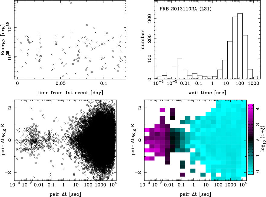
Figure 1: Time-energy space correlation analysis for the FRB 20121102A L21 data. The $t$-$E$ plot of events on the day with the highest event rate (upper-left), the wait time distribution (upper-right), the $\Delta t$-$\Delta\lg E$ plot of pairs (lower-left), and the correlation function in $\Delta t$-$\Delta\lg E$ space (lower-right) are shown.

For the difference of time ($\Delta t\equiv t_{2}-t_{1}$, $t_{2}>t_{1}$) and energy ($\Delta\lg E\equiv\lg E_{2}-\lg E_{1}$, where $\lg=\log_{10}$) of a burst pair (burst 1 and 2), the two-point correlation function $\xi(\Delta t,\Delta\lg E)$ is defined as the excess of the number of pairs $N_{p}$ over the uncorrelated case:

$$dN_{p}=(1+\xi)\,\bar{n}_{p}\,d(\Delta t)\,d(\Delta\lg E)\ ,$$ (1)

where $\bar{n}_{p}$ is the expected pair number density in the uncorrelated case.

The method of estimating the correlation function is widely used in cosmology to study the spatial correlation of galaxies, and has been described in many references [e.g. §16.7 of Peacock (1999)]. The two-point correlation function is estimated by counting the number of pairs consisting of two objects and comparing them to a random sample made up of uncorrelated objects. To reduce statistical error, random data are usually generated with a much larger number of objects than the observed data, and in this study, the random sample is 100 times larger ($10^{4}$ times larger in terms of the number of pairs). The number of all possible pairs involved in a given bin of $\Delta t$-$\Delta\lg E$ space is denoted as $DD$ for the real data sample and $RR$ for the random sample, where $DD$ and $RR$ are appropriately normalized for different sample sizes. Then the correlation function can be estimated as

$$\xi(\Delta t,\Delta\lg E)=\frac{DD}{RR}-1\ ,$$ (2)

but here we use

$$\xi(\Delta t,\Delta\lg E)=\frac{DD-2DR+RR}{RR}\ ,$$ (3)

which is an estimator that has less variance and is most widely used (Landy & Szalay, 1993), where $DR$ is the number of cross-pairs between the data and random samples. (We confirmed that using the former “natural” estimator has little effect on the conclusions of this paper.) The time correlation function $\xi(\Delta t)$ is estimated in the same way, but without binning to the energy direction.

The random data to calculate $\bar{n}_{p}$ were generated as follows. The observation period for a single FRB data set spans multiple days, but a continuous observation is only a few hours per day. Therefore, we assume that it is a Poisson process with a constant rate and a constant energy distribution within a day. There are occasional interruptions during one day of observation, and these were taken into account in the random data generation according to the observation logs. The energy $E$ of the random data was generated assuming a cumulative distribution $f({<}E)$, which was empirically constructed from the observed energies as $f({<}E_{i})=i/(1+N)$ ($i=0,\dots,N+1$), where $f({<}E)$ is linearly interpolated between $E_{i}<E<E_{i+1}$. Here, $E_{i}$ are the energies (in increasing order) of the observed $N$ event in one day for $i=1,\dots,N$, and we set $E_{0}=E_{1}-\delta E$ and $E_{N+1}=E_{N}+\delta E$, where $\delta E=(E_{N}-E_{1})/(N-1)$ is the mean energy separation. Pairs across different days were not considered. Then pair counts within a day were added up for all observed days to compute the correlation function for a single data set.

The simplest way to estimate the correlation function errors is by Poisson error for the pair counts. However, if the correlation is nonzero, the Poisson error is a lower bound to the real error, and furthermore, errors between different bins are correlated. We, therefore, computed the covariance matrix $C_{ij}$ of $\xi(\Delta t)$ using the jackknife method (Norberg et al., 2009) by dividing the observation time of each day into 20 segments, where $i$ and $j$ denote the bins of $\Delta t$. The error $C_{ii}^{1/2}$ for the $i$-th $\Delta t$ bin determined by this method is not significantly different from that evaluated by Poisson statistics. Jackknife errors are sometimes smaller than Poisson errors, which is probably due to a sampling bias. Therefore, the larger of Poisson and jackknife errors are conservatively shown at each data point when errors of $\xi(\Delta t)$ are presented.

The catalog of time and energy obtained from observations is subject to bias due to selection effects. The most obvious effect is that bursts of weak radio fluxes are below the detection limit and do not enter the sample. However, since we are empirically constructing the energy distribution function for the random samples from the observed data, the incompleteness with respect to energy is correctly taken into account here. Another important effect is that when two independent events occur in close proximity in time, they are indistinguishable from sub-bursts within a single event, or the detection sensitivity to fainter bursts is reduced. This effect is, in fact, important in the FRB samples analyzed here, and it will be discussed in detail in the next section.

2.3 Results

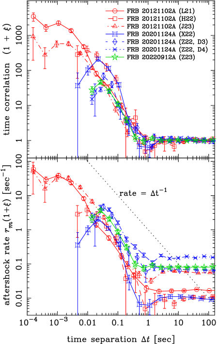
Figure 2: The time correlation function $\xi(\Delta t)$ of the seven FRB data sets. The upper panel shows $(1+\xi)$, while the lower panel shows $r_{m}(1+\xi)$, the aftershock rate occurring $\Delta t$ after an event, where $r_{m}$ is the mean event rate.

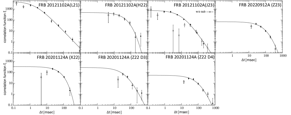
Figure 3: Model fits to the time correlation functions of FRBs. To avoid the effects of removing sub-bursts, open-circle data points were not used for fitting. For the FRB 20121102A (J23) data, two cases are plotted: one in which all sub-bursts are considered (filled and open circles, the fit is to this case), and the other in which only the first sub-burst of a single independent event is considered (crosses).

Figure 1 shows the event distribution in $t$-$E$ space, the wait time distribution, and the pair distribution and correlation function $\xi$ in $\Delta t$-$\Delta\lg E$ space for the FRB 20121102A L21 data set (the other six are shown in Figs. 10–15 in Appendix A).

The time correlation functions $\xi(\Delta t)$ for the seven data sets are shown together in Fig. 2 and separately in Fig. 3. No clear signal in the $\Delta t>1$ s region indicates that the uncorrelated Poisson process can describe the data, which confirms previous studies. On the other hand, clear correlation signals are detected for all the data sets at $\Delta t\lesssim 1$ s, corresponding to the shorter side of the bimodal wait time distribution. These signals exhibit power-law behavior in $\Delta t\sim$ 0.01–1 s, but are flatter in the shortest $\Delta t$ region. In the region of $\Delta t\lesssim$ 0.01 s, the signal behavior differs among the seven data sets, likely due to different treatments about sub-bursts in a single event. In general, if the radio flux rises again before falling to noise levels, it is considered a sub-structure within a single event. However, the exact criteria and whether to include sub-bursts in the catalog are not standardized (Hewitt et al., 2022; Jahns et al., 2023). This effect is clearly seen in the FRB 20121102A (J23) data set, where every sub-burst is explicitly listed in the catalog. When only the first sub-burst of an independent event (849 in total) is used in the analysis, $\xi$ becomes flat below 30 msec, whereas $\xi$ continues to increase smoothly with decreasing $\Delta t$ until 1 ms when all 1,027 sub-bursts are used (Fig. 3). This suggests that even those classified as sub-bursts might be better treated as independent events.

We fit these signals with the function

$$\xi(\Delta t)=C\,\frac{(\Delta t+\tau)^{-p}}{\tau^{-p}}\ ,$$ (4)

by minimizing $\chi^{2}$. Ideally, $\chi^{2}$ should be calculated using the inverse of the covariance matrix (Norberg et al., 2009), $C^{-1}_{ij}$, but it is known that when the sample size is limited, inverting $C_{ij}$ estimated by jackknife can be numerically unstable (Okumura et al., 2008; Pope & Szapudi, 2008). In fact, we found that $\chi^{2}$ using $C_{ij}^{-1}$ varies sensitively with changes in the analysis parameters (e.g. binning), and reliable results could not be obtained. Since a precise determination of the model parameter values is not the main purpose of this study, error correlations between different $\Delta t$ bins were not considered, and the larger of the Poisson and jackknife errors were employed for the error of the $i$-th $\Delta t$ bin. Perhaps the best way to properly incorporate error correlation is to perform Monte Carlo simulations with realistic theoretical modeling, which is beyond the scope of this study. The upper and lower 1$\sigma$ (68% CL) limits for the three model parameters ($C$, $p$, and $\tau$) were determined by the excess $\Delta\chi^{2}$ from the minimum, which is expected to follow a $\chi^{2}$ distribution with three degrees of freedom.

As seen in the case of FRB 20121102A (J23) (Fig. 3), the artificial effect of sub-burst removal results in a sharp drop of $\xi(\Delta t)$ in the smallest $\Delta t$ region. The drops seen in other data sets are also likely due to this effect, and fitting the functional form of eq. (4) to such a data set may produce biased results. Therefore, we excluded data points at $\Delta t$ smaller than the peak of $\xi(\Delta t)$ from the fit. In the large $\Delta t$ region ($\gtrsim$ 1 s), no significant correlation signals are found. However, because of the large number of available pairs in this region, the statistical errors are very small, and consequently the fit becomes sensitive to systematic uncertainties. In particular, our analysis assumes that the burst rate is constant within a day, but if the actual rate is slowly changing on a time scale of about a day, it may appear as a non-zero signal in the correlation function. We are interested in the $\xi$ signal clearly detected at $\Delta t<1$ s, and since it decreases rapidly as $\Delta t$ increases, the signal is hidden by noise in large $\Delta t$ regions. Therefore, data at $\Delta t$ larger than the point at which $\xi$ first becomes negative were excluded from the fit.

The best-fit parameter values and their errors of $C$, $p$, and $\tau$ are shown in Table 1, and the best-fit curves are shown in Fig. 3. The power law fits are particularly good for the two data sets (FRB 20121102A L21 and J23) extending to small $\Delta t$ comparable with typical FRB durations (1–10 msec), with the index $p\sim$ 1.6 or 2.3. The fact that $p$ is restricted to a relatively narrow range indicates that these data cannot be fitted by other function forms, such as the exponential function. For the FRB 20201124A (Z22 D3) data, pure power-law without the effect of non-zero $\tau$ is also consistent with the data within 68% CL, and no lower bound on $\tau$ (and corresponding upper bound on $C$) can be placed.

The data sets other than FRB 20121102A (L21) and (J23) are likely biased toward larger $\tau$ because small $\Delta t$ pairs have been removed as sub-bursts, thus making the power-law features less clear. However, the power-law with $p\sim 2$ is within the 1$\sigma$ error range for all FRB data sets except for FRB 20201124A (X22). The $p$ value of the X22 data may be significantly larger than those in other sets, but it is due to the only data point with a large error at $\Delta t=$ 230 msec (Fig. 3), and hence the possibility of statistical fluctuation cannot be ruled out. The lower limits of 2 and 3$\sigma$ are $p=$ 3.0 and 2.1, respectively, for the X22 data. It should also be noted that $p$ tends to be larger when $\tau$ is large due to degeneracy in the fit (see the next paragraph), and both $\tau$ and $p$ may be biased to a greater value because of sub-burst removal.

As for the upper limits on $p$, the data sets other than FRB 20121102A (L21) and (J23) are consistent with extremely large values of $p>30$ within $1\sigma$. This means that $\xi(\Delta t)$ can also be fitted with an exponential function, because the fitting function converges into $\exp(-\Delta t/\tau^{\prime})$ in the limit of $\tau\rightarrow\infty$ and $p\rightarrow\infty$ with $\tau^{\prime}=\tau/p$, which can be shown as

$$\frac{\xi(\Delta t)}{C}=\left(1+\frac{\Delta t}{\tau}\right)^{-p}=\left(1+\frac{1}{\alpha}\right)^{-\alpha(\Delta t/\tau)p}\rightarrow\exp\left(-\frac{\Delta t}{\tau^{\prime}}\right)\ ,$$ (5)

where $\alpha\equiv\tau/\Delta t$. Our parameter search is limited to $p\leq 30$, and if $p=30$ falls within the 1$\sigma$ error region, “$p>30$” and the corresponding value of $\tau$ are indicated in Table 1 as 1$\sigma$ upper bounds, but this is essentially an exponential fit with $\exp[-\Delta t/(\tau/p)]$.

In summary, at least two of the data sets show clear power laws of $p\sim 2$, and the other data sets are consistent with similar power laws. The power law feature indicates that there is no characteristic time scale for the correlation. It is then natural to assume that the shorter peak of the bimodal wait-time distribution does not reflect the activity duration, but rather correlated aftershocks like earthquakes. In fact, it is known that the aftershock occurrence rate of earthquakes follows a power-law $\propto(\Delta t+\tau)^{-p}$ with $p\sim 1$ (the Omori-Utsu law) (Omori, 1894; Utsu, 1957, 1961; Utsu et al., 1995; de Arcangelis et al., 2016). This consideration provides a good motivation to investigate the similarity of correlation functions between FRBs and earthquakes.

3 Comparison with earthquakes and solar flares

3.1 The earthquake data sets

Table 2: Summary of the earthquake data sets

Name	Longitude	Latitude	Period	${t_{\rm obs}}^{a}$	Events	${r_{m}}^{b}$	${C_{\mathrm{best}}}^{c}$	$p_{\mathrm{best}}$	$\tau_{\mathrm{best}}$	$n^{d}$
	(deg)	(deg)	(MJD)	(day)		(day-1)	$C_{-1\sigma}$	$p_{-1\sigma}$	$\tau_{-1\sigma}$
							$C_{+1\sigma}$	$p_{+1\sigma}$	$\tau_{+1\sigma}$
Narita b311e	140.10–140.70	35.70–36.10	52500–53500	1000	938	1.1	42	0.88	112	0.31
							22	0.73	20	0.60
							110	1.1	460
Narita a311e	140.10–140.70	35.70–36.10	55700–55900	200	997	5.2	5.8	1.1	270	0.15
							3.2	0.75	80	0.32
							12	2.3	1800
Choshi	140.81–140.96	35.74–35.86	52500–55600	3100	800	0.35	130	1.0	180	0.37
							62	0.87	20	0.51
							370	1.37	740
Kanto	139.30–141.10	35.00–36.00	53000–53500	500	1399	2.9	34	0.75	16	0.17
							16	0.7	2.0	0.44
							152	0.87	64
Izumo	132.20–132.60	34.70–35.50	52500–55500	3000	1596	0.57	380	0.82	5.0	0.18
							140	0.72	0.6	0.34
							1800	0.98	24

^aTotal observation time
^bMean event rate weighted by the number of pairs for all 10 partial periods
^cThe best-fit value, 68% CL lower and upper limits of the parameters $C$, $p$, and $\tau$ (in [s])
^dThe branching ratio with the integration upper bound of $\Delta t_{u}$ where $\xi(\Delta t_{u})=1$ (top) or 0.1 (bottom)
^eBefore and after the Tohoku earthquake on March 11, 2011.

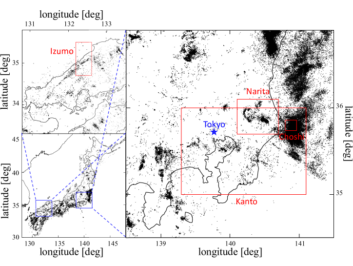
Figure 4: Map of regions from which the earthquake data were extracted. Distributions of epicenters during a period (May 6, 2010 – December 31, 2012) are shown by dots.

To quantify the similarity to earthquakes, we used the same analysis method to examine time-energy correlations of earthquakes. The earthquake data used in this study were extracted from the Japan Unified hI-resolution relocated Catalog for Earthquakes (JUICE, Yano et al. 2017). Five data sets of similar sample sizes to FRBs ($\sim$ 1,000 events for each data set) were extracted from various regions, area sizes, and time periods (Table 2). The three regions of Choshi, Narita, and Izumo were selected to see the regional dependences, and data from the greater Kanto region (including Choshi and Narita) were also analyzed to see the dependence on area size (Fig. 4). To keep the sample size similar to that of FRBs, the time period was adjusted so that the number of events in each data set is approximately 1,000. The rate of earthquakes changed dramatically before and after the huge Tohoku earthquake on March 11, 2011. We analyzed data from Narita before and after this to see the impact of the change in activity. The other three data sets are all before the earthquake.

The energy of earthquakes was calculated from the magnitude by the formula $E=10^{11.8+1.5M}$ erg. Magnitudes in the catalog are discretized with an accuracy of 0.1, and they are shifted randomly with an amplitude of less than $\pm$0.05 to avoid creating pairs with exactly zero energy differences. Unlike FRBs, observations of earthquakes and solar flares were made continuously 24 hours a day. However, to make the analysis as similar as possible to FRBs, we divided a data set into 10 equal partial periods, with each corresponding to a single date of FRB observations. As with FRBs, pairs were looked for only within partial periods, and pair counts were added up over the entire period to compute $\xi$. Results for the Narita b311 data are shown in Fig. 5, and those of the other four sets are in Figs. 16-19 in Appendix A.

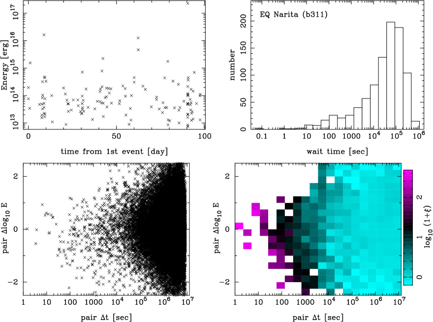
Figure 5: The same as Fig. 1, but for the Narita (before 311) earthquake data.

3.2 FRBs versus earthquakes

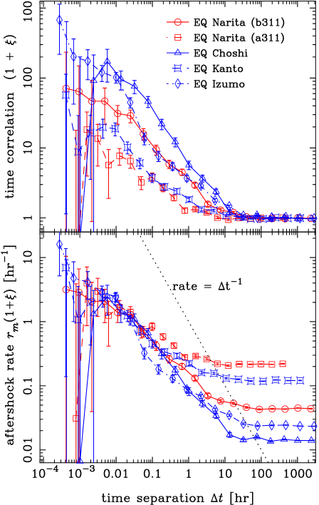
Figure 6: The same as Fig. 2, but for the earthquake data.

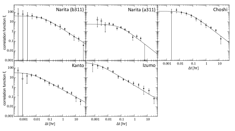
Figure 7: The same as Fig. 3, but for the earthquake data.

The time correlation functions of the earthquake data sets are shown in Figs. 6 and 7. They are similar to FRBs in that $\xi(\Delta t)$ is a power law of $\propto(\Delta t+\tau)^{-p}$ at small $\Delta t$ but uncorrelated events at a constant rate become dominant in the large $\Delta t$ region. Denoting $r_{m}$ as the mean event rate including uncorrelated events (shown in Table 1 and Table 2), $(1+\xi)\,r_{m}$ becomes the aftershock rate, i.e., the rate of events occurring $\Delta t$ after an event, by definition of the correlation function. This is shown in the bottom panel of Figs. 2 (FRBs) and 6 (earthquakes). Since FRB event rates vary on different observation dates within a single data set, we calculated $r_{m}$ for the entire data set by taking an average weighted by the number of pairs on each date (or partial period in earthquake data).

The expected number of correlated aftershocks to an event (called “the branching ratio” in earthquake studies) is given by $n\equiv\int r_{m}\,\xi(\Delta t)\,d(\Delta t)$, and if $n$ is less than 1, the effect of a single event causing multiple aftershocks is small. The condition for $n<1$ is roughly $r_{m}\,\xi<(\Delta t)^{-1}$, which is satisfied in both the FRB and earthquake data, as seen in Figs. 2 and 6. The branching ratio $n$ was calculated using the best-fit parameter values of $\xi(\Delta t)$, and shown in Tables 1 and 2. Since $p$ is smaller than 1 in some of the earthquake data sets, the upper bound $\Delta t_{u}$ of the integration for $n$ was set to the point where $\xi(\Delta t_{u})=1$ or 0.1 to avoid divergence. The values of $n$ are indeed less than 1, but of order unity ($\gtrsim$ 0.1) for all FRB and earthquake data sets.

Then these results can be interpreted as each event produces at most one aftershock at a rate consistent with the Omori-Utsu law, $r_{m}\,\xi\propto(\Delta t+\tau)^{-p}$, where all events are treated on the same footing and there is no distinction between mainshocks and aftershocks. Such a model is called ETAS (epidemic-type aftershock sequence) in earthquake studies and is known to explain earthquake data well (Ogata, 1999; Saichev & Sornette, 2006; de Arcangelis et al., 2016).

Further similarities between FRBs and earthquakes can be pointed out. The branching ratio $n$ is about 0.1–0.5 for both FRBs and earthquakes (Tables 1 and 2), which is also similar to those found in past earthquake studies (Saichev & Sornette, 2006; de Arcangelis et al., 2016). The power law flattens at $\Delta t\lesssim\tau$, and $\tau$ is about 1–10 msec for FRBs and 0.3–3 min for earthquakes, which are close to the typical duration of the respective phenomena. It should also be noted that the correlated aftershock rate ($r_{m}\,\xi$) is stable both in FRBs and earthquakes (bottom panels of Figs. 2 and 6), even though the mean event rate $r_{m}$ of uncorrelated events varies widely with changes of source activity (and also with the choice of region and its area size for earthquakes). The aftershock rates of the three different FRB sources are not significantly different, but the rate fluctuations are even smaller within each source. This indicates that aftershocks are not caused by the activity of the source as a whole, but by the changes induced by each individual event. Finally, there is little correlation between $\Delta t$ and $\Delta\lg E$ in either FRBs or earthquakes ($\xi$ almost constant against $\Delta\lg E$ in Figs. 1, 5, and 10–19).

In fact, a slight time-magnitude correlation has been reported by detailed statistical tests for earthquakes (Lippiello et al., 2008; de Arcangelis et al., 2016; Zhang et al., 2023b). Asymmetry with respect to $\Delta\lg E$ (more negative $\Delta\lg E$ pairs, i.e., aftershock energy smaller than mainshock) may also be evident in some of our earthquake data sets: Narita (b311, Fig. 5), Choshi (Fig. 17), and Izumo (Fig. 19). Similar asymmetry about $\Delta\lg E$ is not visible in the FRB data, but it may be due to a narrow dynamic range of $E$ caused by detection limits. Careful verification by future studies would be desirable.

The only difference between the two phenomena is the value of the Omori-Utsu index, $p$: FRBs have a larger $p$ resulting in the bimodal wait-time distribution, while bimodality is not clearly visible in the earthquake data. It should be noted, however, that $p$ of earthquake data varies widely depending on regions, and those of FRBs are marginally within the range for earthquakes ($p=$ 0.6–1.9) reported by past studies (Utsu et al., 1995; Ogata, 1999; Wiemer & Katsumata, 1999; de Arcangelis et al., 2016).

3.2.1 Notes on previous studies on the Omori-Utsu law in neutron star phenomena

Wang et al. (2018) found that the rate evolution of 14 bursts detected during an observation of about 60 minutes from FRB 20121102A is consistent with the Omori-Utsu law. This result is likely unrelated to the correlations found in this study because the correlation time scale of Wang et al. (2018) is much larger than $\Delta t\sim$ 1 s, where we did not find significant correlations. It is difficult to draw strong conclusions from the sample of Wang et al. (2018), not only because of the small statistics but also because of the arbitrariness of where to separate mainshocks and aftershocks. It is possible that the rate variation observed by Wang et al. (2018) does not reflect a systematic aftershock sequence, but rather a change in the source activity during that observation period.

Enoto et al. (2017) analyzed the light curves of X-ray outbursts in three magnetars and found that they can be fitted by the Omori-Utsu law, and proposed the possibility that X-ray luminosity is superpositions of many small starquakes. However, the plateau time scale $\tau$ is longer than 10 days, which is many orders of magnitude larger than the time correlations found in this work, suggesting that there is no direct relationship between the two. It should be noted that continuous luminosity evolution can also be explained by continuous evolution of energy release in a single system, rather than by the superposition of many discrete aftershocks. In general, in systems where the energy loss rate $\dot{E}$ is proportional to the power of the system energy $E$ ($\dot{E}\propto E^{q}$), the evolution of $\dot{E}$ takes the form of the Omori-Utsu formula with $p=q/(q-1)$ (e.g., $q=2$ for a rotation-powered pulsar with a constant magnetic field strength).

3.3 Comparison with solar flares

The solar flare data were taken from the Hinode catalog (Watanabe et al., 2012). To see the dependence on activity level, data were extracted from two periods (200 days from 2012 Apr. to Oct., and 1,200 days from 2017 Oct. to 2021 Jan.) of high and low solar activity, adjusting the time period so that each period includes about 1,000 events (1,422 and 1,207 events, respectively). The X-ray flux was calculated from the flare class in the catalog, and this was used as a proxy for energy $E$. Flare classes are given as two significant digits and, as with the earthquake data, they were randomly shifted by the precision of the significant digits [e.g., X-ray flux of a B4.2 class flare is randomly chosen from the range of $(4.15$–$4.25)\times 10^{-4}\ \rm erg\ cm^{-2}\ s^{-1}$]. These data sets were analyzed in the same way as earthquakes, and the results for the low activity set is shown in Fig. 8 (and the high activity set in Fig. 20 in Appendix A). Time correlation functions for the two sets are shown in Fig. 9.

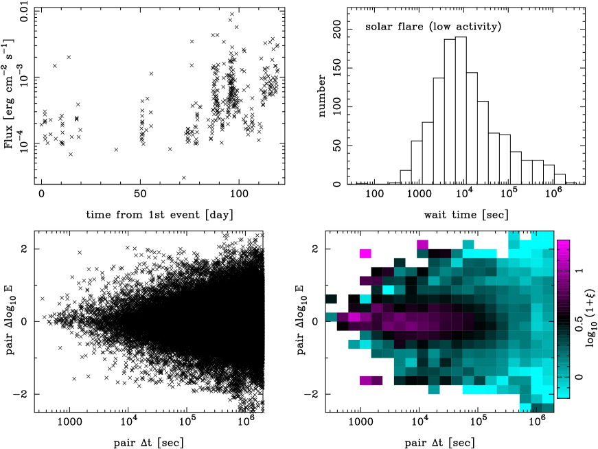
Figure 8: The same as Fig. 1, but for the solar flare (low activity) data.

Figure 9 shows that a significant time correlation signal is detected in the region of $\Delta t\lesssim 100$ hr. It is known that flares occurring in different active regions on the solar surface are uncorrelated (Benz, 2017), and hence the correlated signals are thought to be between flares occurring in a common active region. We can convert $\xi$ into the correlated aftershock rate $r_{m}\,\xi$, and it is stable regardless of the level of solar activity ($r_{m}$), which is similar to the behaviors of FRBs and earthquakes. However, $\xi$ reaches at most 5 without showing a clear power law, in sharp contrast to FRBs and earthquakes. The correlated rate $r_{m}\,\xi$ is well above $(\Delta t)^{-1}$, which indicates that the branching ratio $n$ is larger than 1 and multiple aftershocks are generated from a single event. Another difference from FRBs or earthquakes is the strong correlation not only in time but also in energy, with $\xi$ peaking at $\Delta t\sim 10^{3}$–$10^{4}$ s and $\Delta\lg E\sim 0$ (lower-right panels of Figs. 8 and 20). This strong time-energy clustering nature is evident in the $t$-$E$ distribution shown in these figures (upper-left panels), which are not seen in FRB or earthquake data.

Though similarities between solar flares and magnetars are often discussed, these results indicate a different nature of the time-energy correlation of solar flares compared to FRBs and earthquakes. Interpretation of these results in comparison with the physics and theory of solar flares is outside the scope of this study. Time and/or energy correlations of solar flares have been discussed by analyzing the wait time distributions and cross-correlations between energy and time (either since the last event or to the next event) (Wheatland, 2000; Lippiello et al., 2010; Hudson, 2020; Carlin et al., 2023). It is not straightforward to compare our results with these, because $\Delta t$ in our analysis is not wait time but time separation for arbitrary pairs, and we are looking at the energy difference $\Delta\lg E$ of an event pair, rather than the energy itself of one event. Careful comparison of these results to elicit information about the physics of solar flares is an interesting subject for future research. In such studies, it is important to take into account observational biases in the solar flare catalog, such as the obscuration effect (lower detection efficiency for faint flares after a giant flare, Wheatland 2001).

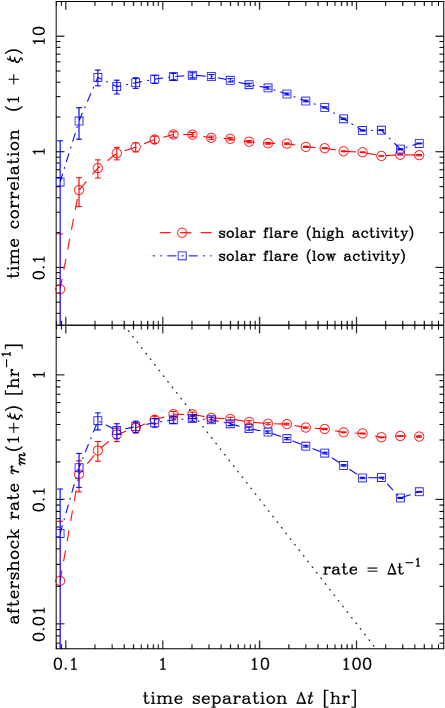
Figure 9: The same as Fig. 2, but for the solar flare data.

4 Conclusions and Discussion

By examining the correlation functions in time-energy space, we found remarkable similarities between the statistical properties of FRBs and earthquakes, especially the laws on aftershock occurrence. Listing the similarities, (1) the aftershock rate follows a power law of $\propto(\Delta t+\tau)^{-p}$ (the Omori-Utsu law), (2) $\tau$ is about the same as the typical event duration, (3) the branching ratio (expected number of aftershocks associated with a single event) is $n=0.1$–0.6 for both phenomena, (4) the correlated aftershock rates remain stable regardless of the change in the source activity or mean event rate, and (5) there is little correlation between energy and time.

In contrast, the correlation functions for solar flares differ significantly from those of FRBs and earthquakes. The correlation function cannot be fitted by a power law, and the branching ratio is significantly greater than unity, which means that a single event causes multiple aftershocks. There is also a strong correlation in the direction of energy, with flares of similar energy tending to occur in succession. It is well known that the energy distribution of solar flares follows a power law, which is often noted to be similar to that of earthquakes (the Wadati-Gutenberg-Richter law, Wadati 1932; Gutenberg & Richter 1944). However, with respect to correlations in the time-energy space, solar flares do not resemble earthquakes, and by comparison, the similarity between FRBs and earthquakes is remarkable.

Both solar flares and magnetars are caused by magnetic energy, but unlike the Sun, neutron stars are thought to have solid crusts on their surfaces. Therefore, the most natural interpretation of the present results is that FRBs are earthquake-like phenomena that suddenly release the energy stored in neutron star crusts. Other models of FRB repeaters are not immediately dismissed, but any model must be consistent with this time-energy correlation, placing strong constraints on possible models.

In the case of earthquakes, differences in the index $p$ are thought to reflect the physical properties of crust and seismic processes (Ogata, 1999; Wiemer & Katsumata, 1999; de Arcangelis et al., 2016). Then relatively large $p$ values of FRBs may provide information about the physical properties of neutron star crusts, and energy production mechanism by seismic processes in them. This suggests a new possibility for future studies to probe the physics of dense nuclear matter by using repeater FRBs.

Two FRB repeaters, including 20121102A, are known to periodically change their activity in cycles of 16 or 160 days (Amiri et al., 2020; Rajwade et al., 2020; Cruces et al., 2021). If these are neutron stars in a binary system, the activity may be increased when the crust is deformed by tidal forces from the companion star at the pericenter. Models of binary origin have been proposed for the periodic FRB activities (Ioka & Zhang, 2020; Lyutikov et al., 2020; Barkov & Popov, 2022), but most have assumed that the periodicity is due to the absorption of FRB radiation (e.g. by stellar winds from the companion star), rather than intrinsic change of the FRB production activity. A repeater FRB has been found in a globular cluster of the nearby galaxy M81 (Kirsten et al., 2022), and the FRB activity may be stimulated by close encounters with other stars in the cluster.

As far as we know, most previous studies on the time correlation of earthquakes or solar flares have also been based on wait times rather than correlation function (de Arcangelis et al., 2016; Saichev & Sornette, 2006; Wheatland, 2000). The correlation function method adopted here fully exploits the temporal information of the sample, and the time dependence of the correlated aftershock rate can be seen more directly. This is why the two phenomena (FRBs and earthquakes), that appear to be different in the wait time distribution, turn out to have essentially the same properties when viewed in terms of the correlation function. Applying this method to a wider range of earthquake and solar flare data may provide new insights into these phenomena.

Data Availability

The data newly derived in this article (e.g., correlation function values) will be shared on reasonable request to the corresponding author.

Appendix A Figures of detailed results for the data sets not presented in the main part

Figures of detailed results ($t$-$E$ scatter plot, wait-time distribution, pair distribution and correlation function in $\Delta t$-$\Delta\lg E$ space) for each data set were presented only for FRB 20121102A (L21, Fig. 1), earthquake Narita (b311, Fig. 5), and solar flare (low activity, Fig. 8) in the main part. Here figures for other data sets are presented as Figs. 10–20.

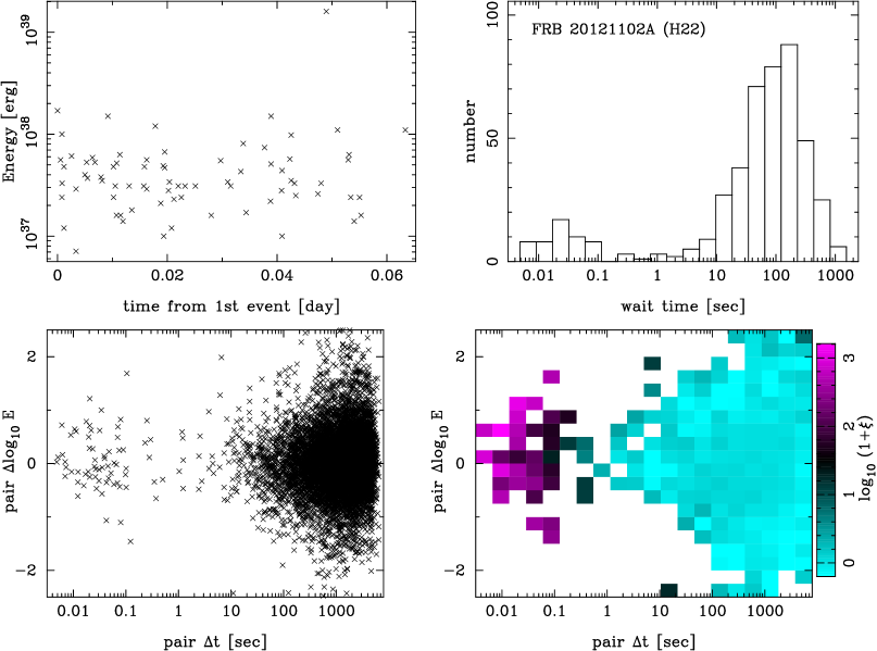
Figure 10: The same as Fig. 1, but for the FRB 20121102A (H22) data.

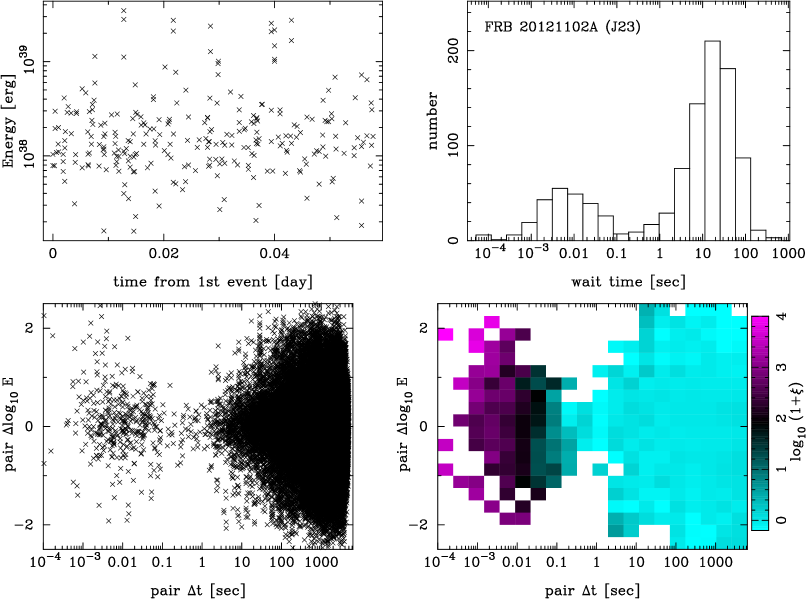
Figure 11: The same as Fig. 1, but for the FRB 20121102A (J23) data.

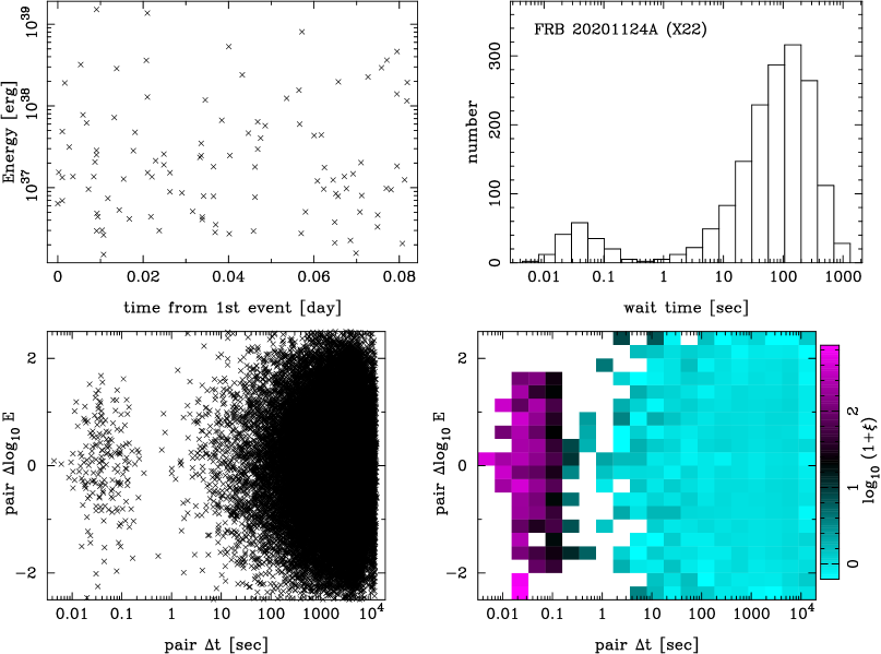
Figure 12: The same as Fig. 1, but for the FRB 20201124A (X22) data.

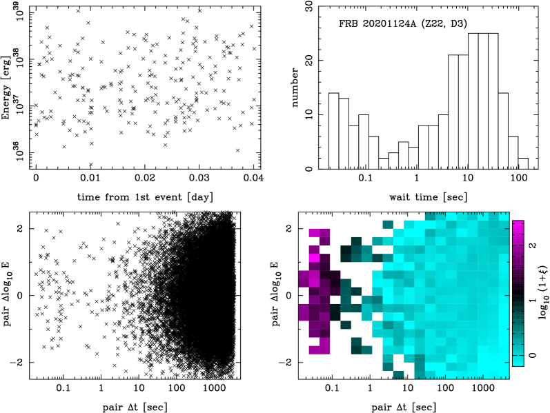
Figure 13: The same as Fig. 1, but for the FRB 20201124A (Z22, D3) data.

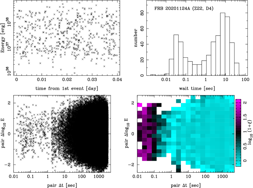
Figure 14: The same as Fig. 1, but for the FRB 20201124A (Z22, D4) data.

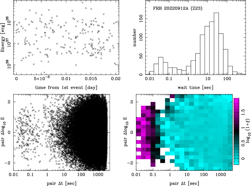
Figure 15: The same as Fig. 1, but for the FRB 20220912A (Z23) data.

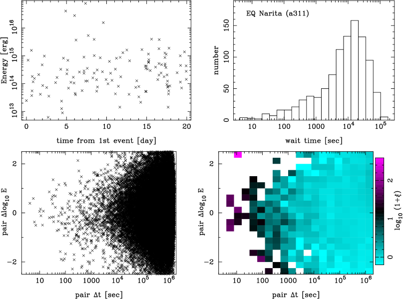
Figure 16: The same as Fig. 1, but for the Narita (after 311) earthquake data.

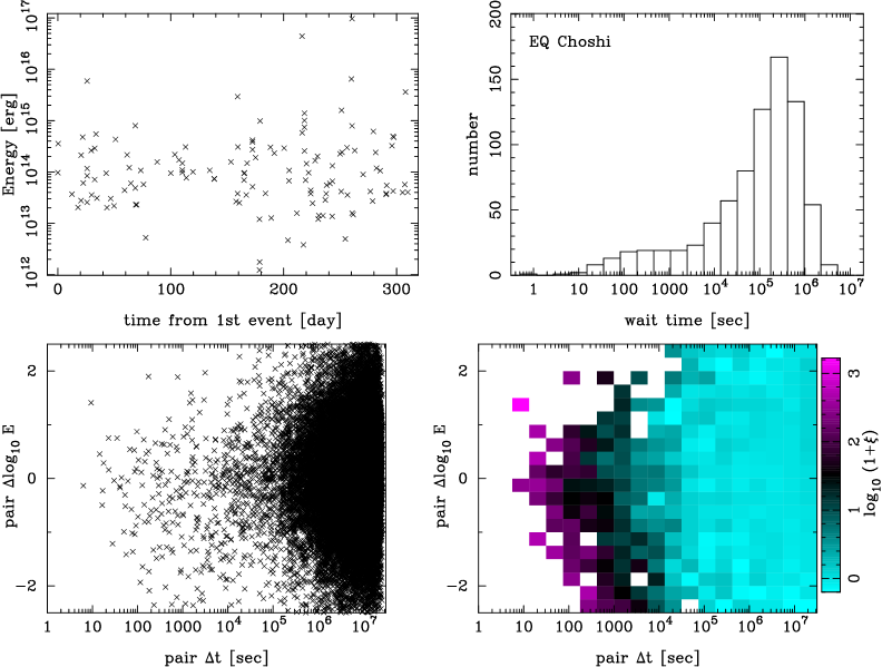
Figure 17: The same as Fig. 1, but for the Choshi earthquake data.

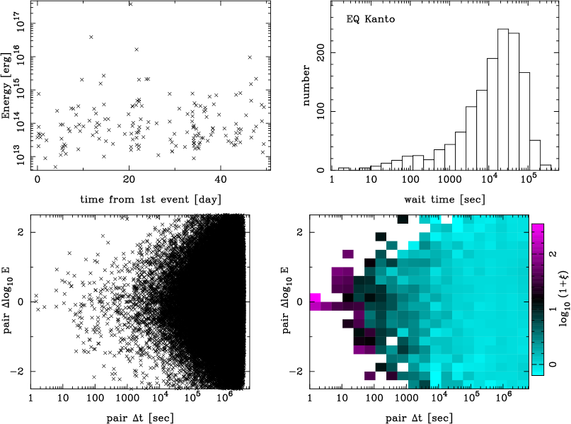
Figure 18: The same as Fig. 1, but for the Kanto earthquake data.

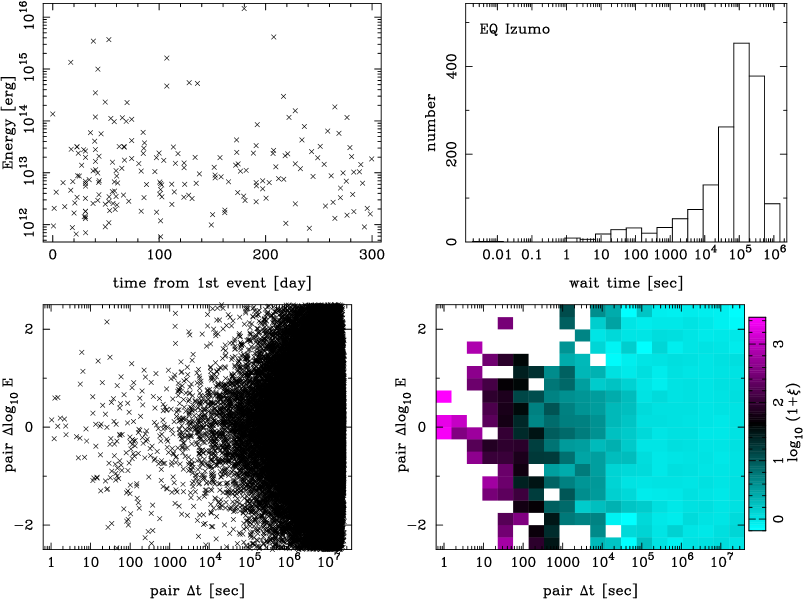
Figure 19: The same as Fig. 1, but for the Izumo earthquake data.

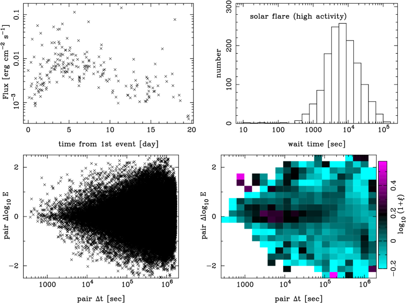
Figure 20: The same as Fig. 1, but for the solar flare (high activity) data.

References

- Aggarwal et al. (2021) Aggarwal K., Agarwal D., Lewis E. F., Anna-Thomas R., Tremblay J. C., Burke-Spolaor S., McLaughlin M. A., Lorimer D. R., 2021, ApJ, 922, 115
- Amiri et al. (2020) Amiri M., et al., 2020, Nature, 582, 351
- Barkov & Popov (2022) Barkov M. V., Popov S. B., 2022, MNRAS, 515, 4217
- Bassa et al. (2017) Bassa C. G., et al., 2017, The Astrophysical Journal, 843, L8
- Benz (2017) Benz A. O., 2017, Living Reviews in Solar Physics, 14, 2
- Bochenek et al. (2020) Bochenek C. D., Ravi V., Belov K. V., Hallinan G., Kocz J., Kulkarni S. R., McKenna D. L., 2020, Nature, 587, 59
- Carlin et al. (2023) Carlin J. B., Melatos A., Wheatland M. S., 2023, ApJ, 948, 76
- Chatterjee et al. (2017) Chatterjee S., et al., 2017, Nature, 541, 58
- Cheng et al. (1996) Cheng B., Epstein R. I., Guyer R. A., Young A. C., 1996, Nature, 382, 518
- Cordes & Chatterjee (2019) Cordes J. M., Chatterjee S., 2019, Annual Review of Astronomy and Astrophysics, 57, 417
- Cruces et al. (2021) Cruces M., et al., 2021, Monthly Notices of the Royal Astronomical Society, 500, 448
- Du et al. (2023) Du Y., Wang P., Song L., Xiong S., 2023, arXiv e-prints, p. arXiv:2305.04738
- Enoto et al. (2017) Enoto T., et al., 2017, The Astrophysical Journal Supplement Series, 231, 8
- Gourdji et al. (2019) Gourdji K., Michilli D., Spitler L. G., Hessels J. W. T., Seymour A., Cordes J. M., Chatterjee S., 2019, ApJ, 877, L19
- GöǧüŞ et al. (1999) GöǧüŞ E., Woods P. M., Kouveliotou C., van Paradijs J., Briggs M. S., Duncan R. C., Thompson C., 1999, ApJ, 526, L93
- Gutenberg & Richter (1944) Gutenberg B., Richter C. F., 1944, Bulletin of the Seismological Society of America, 34, 185
- Hewitt et al. (2022) Hewitt D. M., et al., 2022, Monthly Notices of the Royal Astronomical Society, 515, 3577
- Hudson (2020) Hudson H. S., 2020, MNRAS, 491, 4435
- Ioka & Zhang (2020) Ioka K., Zhang B., 2020, ApJ, 893, L26
- Jahns et al. (2023) Jahns J. N., et al., 2023, Monthly Notices of the Royal Astronomical Society, 519, 666
- Kaspi & Beloborodov (2017) Kaspi V. M., Beloborodov A. M., 2017, Annual Review of Astronomy and Astrophysics, 55, 261
- Kirsten et al. (2022) Kirsten F., et al., 2022, Nature, 602, 585
- Landy & Szalay (1993) Landy S. D., Szalay A. S., 1993, The Astrophysical Journal, 412, 64
- Li et al. (2019) Li B., Li L.-B., Zhang Z.-B., Geng J.-J., Song L.-M., Huang Y.-F., Yang Y.-P., 2019, International Journal of Cosmology, Astronomy and Astrophysics, 1, 22
- Li et al. (2021) Li D., et al., 2021, Nature, 598, 267
- Lippiello et al. (2008) Lippiello E., de Arcangelis L., Godano C., 2008, Phys. Rev. Lett., 100, 038501
- Lippiello et al. (2010) Lippiello E., de Arcangelis L., Godano C., 2010, Astronomy and Astrophysics, 511, L2
- Lyutikov et al. (2020) Lyutikov M., Barkov M. V., Giannios D., 2020, ApJ, 893, L39
- McKinven & Chime/FRB Collaboration (2022) McKinven R., Chime/FRB Collaboration 2022, The Astronomer’s Telegram, 15679, 1
- Norberg et al. (2009) Norberg P., Baugh C. M., Gaztañaga E., Croton D. J., 2009, Monthly Notices of the Royal Astronomical Society, 396, 19
- Ogata (1999) Ogata Y., 1999, pure and applied geophysics, 155, 471
- Okumura et al. (2008) Okumura T., Matsubara T., Eisenstein D. J., Kayo I., Hikage C., Szalay A. S., Schneider D. P., 2008, The Astrophysical Journal, 676, 889
- Omori (1894) Omori F., 1894, The journal of the College of Science, Imperial University, Japan, 7, 111
- Oostrum et al. (2020) Oostrum L. C., et al., 2020, A&A, 635, A61
- Oppermann et al. (2018) Oppermann N., Yu H.-R., Pen U.-L., 2018, MNRAS, 475, 5109
- Peacock (1999) Peacock J. A., 1999, Cosmological Physics. Cambridge University Press, Cambridge, England
- Petroff et al. (2022) Petroff E., Hessels J. W. T., Lorimer D. R., 2022, A&ARv, 30, 2
- Platts et al. (2019) Platts E., Weltman A., Walters A., Tendulkar S. P., Gordin J. E. B., Kandhai S., 2019, Phys. Rep., 821, 1
- Pope & Szapudi (2008) Pope A. C., Szapudi I., 2008, Monthly Notices of the Royal Astronomical Society, 389, 766
- Rajwade et al. (2020) Rajwade K. M., et al., 2020, Monthly Notices of the Royal Astronomical Society, 495, 3551
- Ravi et al. (2022) Ravi V., et al., 2022, arXiv e-prints, p. arXiv:2211.09049
- Saichev & Sornette (2006) Saichev A., Sornette D., 2006, Phys. Rev. Lett., 97, 078501
- Sang & Lin (2023) Sang Y., Lin H.-N., 2023, Monthly Notices of the Royal Astronomical Society, 523, 5430
- Spitler et al. (2014) Spitler L. G., et al., 2014, The Astrophysical Journal, 790, 101
- Spitler et al. (2016) Spitler L. G., et al., 2016, Nature, 531, 202
- Tabor & Loeb (2020) Tabor E., Loeb A., 2020, The Astrophysical Journal, 902, L17
- Tendulkar et al. (2017) Tendulkar S. P., et al., 2017, The Astrophysical Journal, 834, L7
- The CHIME/FRB Collaboration (2020) The CHIME/FRB Collaboration 2020, Nature, 587, 54
- The CHIME/FRB Collaboration (2021) The CHIME/FRB Collaboration 2021, The Astrophysical Journal Supplement Series, 257, 59
- Utsu (1957) Utsu T., 1957, Zisin, Ser. 2 (in Japanese), 10, 35
- Utsu (1961) Utsu T., 1961, Geophysical magazine, 30, 521
- Utsu (1999) Utsu T., 1999, pure and applied geophysics, 155, 509
- Utsu et al. (1995) Utsu T., Ogata Y., S R., Matsu'ura 1995, Journal of Physics of the Earth, 43, 1
- Wadati (1932) Wadati K., 1932, Journal of the Meteorological Society of Japan. Ser. II (in Japanese), 10, 559
- Wadiasingh & Timokhin (2019) Wadiasingh Z., Timokhin A., 2019, The Astrophysical Journal, 879, 4
- Wang & Yu (2017) Wang F. Y., Yu H., 2017, J. Cosmology Astropart. Phys., 2017, 023
- Wang et al. (2018) Wang W., Luo R., Yue H., Chen X., Lee K., Xu R., 2018, The Astrophysical Journal, 852, 140
- Wang et al. (2023) Wang F. Y., Wu Q., Dai Z. G., 2023, ApJ, 949, L33
- Watanabe et al. (2012) Watanabe K., Masuda S., Segawa T., 2012, Solar Physics, 279, 317
- Wheatland (2000) Wheatland M. S., 2000, The Astrophysical Journal, 536, L109
- Wheatland (2001) Wheatland M., 2001, Solar Physics, 203, 87
- Wiemer & Katsumata (1999) Wiemer S., Katsumata K., 1999, Journal of Geophysical Research: Solid Earth, 104, 13135
- Xu et al. (2022) Xu H., et al., 2022, Nature, 609, 685
- Yano et al. (2017) Yano T. E., Takeda T., Matsubara M., Shiomi K., 2017, Tectonophysics, 702, 19
- Zhang (2020) Zhang B., 2020, Nature, 587, 45
- Zhang et al. (2018) Zhang Y. G., Gajjar V., Foster G., Siemion A., Cordes J., Law C., Wang Y., 2018, ApJ, 866, 149
- Zhang et al. (2021) Zhang G. Q., Wang P., Wu Q., Wang F. Y., Li D., Dai Z. G., Zhang B., 2021, ApJ, 920, L23
- Zhang et al. (2022) Zhang Y.-K., et al., 2022, Research in Astronomy and Astrophysics, 22, 124002
- Zhang et al. (2023a) Zhang Y.-K., et al., 2023a, arXiv e-prints, p. arXiv:2304.14665
- Zhang et al. (2023b) Zhang Y.-K., Li D., Feng Y., Wang P., Niu C.-H., Dai S., Yao J.-M., Tsai C.-W., 2023b, arXiv e-prints, p. arXiv:2305.18052
- de Arcangelis et al. (2016) de Arcangelis L., Godano C., Grasso J. R., Lippiello E., 2016, Physics Reports, 628, 1