Tart: A plug-and-play Transformer module for
task-agnostic reasoning

Abstract

Large language models (LLMs) exhibit in-context learning abilities which enable the same model to perform several tasks without any task-specific training. In contrast, traditional adaptation approaches, such as fine-tuning, modify the underlying models for each specific task. In-context learning, however, consistently underperforms task-specific tuning approaches even when presented with the same examples. While most existing approaches (e.g., prompt engineering) focus on the LLM’s learned representations to patch this performance gap, our analysis actually reveal that LLM representations contain sufficient information to make good predictions. As such, we focus on the LLM’s reasoning abilities and demonstrate that this performance gap exists due to their inability to perform simple probabilistic reasoning tasks. This raises an intriguing question: Are LLMs actually capable of learning how to reason in a task-agnostic manner? We answer this in the affirmative and propose Tart which generically improves an LLM’s reasoning abilities using a synthetically trained Transformer-based reasoning module. Tart trains this reasoning module in a task-agnostic manner using only synthetic logistic regression tasks and composes it with an arbitrary real-world pre-trained model without any additional training. With a single inference module, Tart improves performance across different model families (GPT-Neo, Pythia, Bloom), model sizes (100M - 6B), tasks (14 NLP binary classification tasks), and even across different modalities (audio and vision). Additionally, on the RAFT Benchmark, Tart improves GPT-Neo (125M)’s performance such that it outperforms Bloom (176B), and is within $4\%$ of GPT-3 (175B).

1 Introduction

Large language models (LLMs) show in-context learning capabilities which enable them to perform a task given only a few examples, without updating the model parameters [Bro+20, Bom+21]. This task-agnostic capability allows for a single model to be applied to a wide range of tasks [Agr+22, Wei+22, Nar+22]. In contrast, traditional task adaptation approaches, such as fine-tuning, update the model parameters for each specific task.

Despite being task-agnostic, in-context learning is seldom the practitioner’s method of choice since it consistently underperforms task-specific adaptation approaches [LAC21, Bro+20]. Most existing works attribute this performance gap to the limited context window of LLMs which can only accommodate a few task examples [Koc+23, Huy23, Liu+22]. However, we show that this gap between in-context learning and fine-tuning approaches exists even when presented with the same task examples.

This observation raises the question whether this performance gap is a generic limitation of task-agnostic methods for adaptation or is it specific to in-context learning? Specifically, can we design adaptation approaches which satisfy the following desiderata:

• Task-agnostic: The same model generalizes across several different tasks.

• Quality: Achieves accuracy competitive with task-specific methods across these different tasks.

• Data-scalable: Learning ability improves with increasing number of task examples.

We first investigate why this quality gap exists. We decompose an LLM’s in-context learning capability into two abilities: learning good representations for the task and performing probabilistic inference, or reasoning, over these representations [03]. Is the gap because the representations do not contain sufficient information or because the LLMs are unable to reason over them?

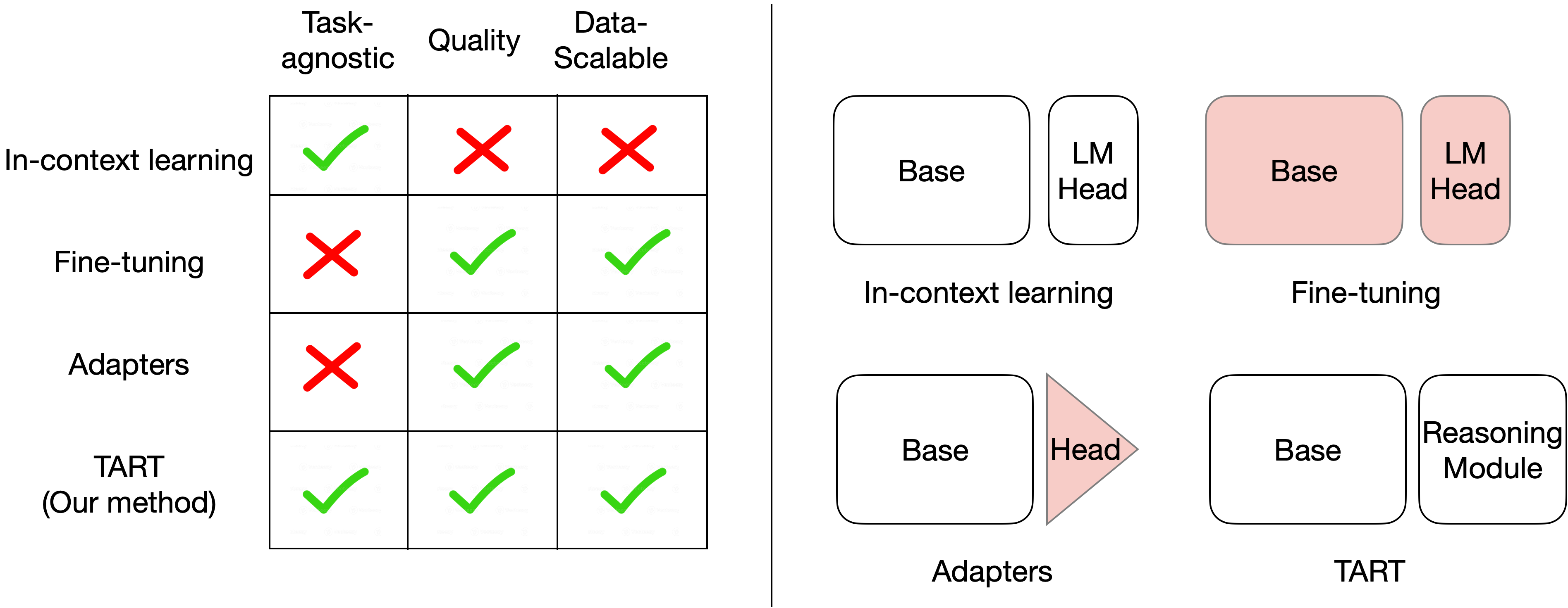
Figure 1: Taxonomy of task adaptation strategies. (Left) Comparison of different adaptation strategies across three desiderata: task-agnostic, quality, scalability. (Right) Parameter updates across adaptations strategies, colored regions represent parameter changes as a result of the adaptation strategy.

We explore this hypothesis experimentally in Section 3 by measuring both the reasoning and the representation gaps across a variety of LLM families (GPT-Neo [Bla+21], Pythia [Bid+23], Bloom [Sca+22]) over a suite of binary classification tasks. We conclude that LLMs possess good representations, and the majority of the quality gap (up to $79$%) can be attributed to their insufficient reasoning ability. We further find that fine-tuning improves the base model on both these axes, but primarily improve the task specific reasoning ability which accounts for $72$% of the gained performance.

Rather surprisingly, most existing techniques for improving the performance gap, such as prompt engineering or active example selection, focus entirely on the LLM’s learned representations. In contrast, our work explores the orthogonal direction of improving the LLM’s reasoning abilities. As a first step, we fine-tune LLMs using synthetically generated probabilistic inference tasks to improve their reasoning capabilities. While this approach provides an improvement over the model’s base in-context learning performance (up to $19$%, see Figure 8 in App. A), this approach requires one to fine-tune each LLM individually. Taking a step further, we consider the possibility of whether one can improve the reasoning capabilities in a manner that is agnostic to both tasks and models.

We show that it is indeed possible to improve the reasoning capabilities in a completely agnostic manner. We propose Tart which improves upon an LLM’s reasoning abilities using a synthetically trained reasoning module (see Figure 2). Tart trains a Transformer-based reasoning module using only synthetically generated logistic regression tasks independent of the downstream task or the base LLM. This inference module can be composed, without any additional training, with the embeddings of an LLM to improve upon its reasoning abilities. Notably, Tart satisfies the desired objectives:

• Task-agnostic: Tart’s inference module is only trained once using synthetic data.

• Quality: Outperforms base LLM on all tasks and closes gap to task specific fine-tuning methods.

• Data-scalable: Can accommodate 10x more examples than in-context learning.

Tart is task, model, and domain agnostic. Using a single inference module trained on synthetic data, we exhibit that Tart not only generalizes across three model families (GPT-Neo, Pythia, Bloom) over 14 NLP classification tasks, but even across different domains (vision and speech; see Figure 7). In terms of quality, we show that Tart’s performance is 18.4% better than in-context learning, 3.4% better than task-specific adapters, and is within 3.1% of full task-specific fine-tuning across a suite of NLP tasks. On the RAFT Benchmark [Ale+21], Tart improves GPT-Neo (125M)’s performance such that it outperforms Bloom (176B), and is within $4\%$ of GPT-3 (175B). Tart is data-scalable and overcomes the limited context length bottleneck of in-context learning. While each example spans multiple tokens in an LLM, often spanning hundreds of tokens, Tart’s reasoning module encodes each example using only two tokens – one for the context and the other for the label. This data-scalability can lead to improvements of up to $6.8\%$ (see Figure 6(c)).

From a theoretical standpoint, we show that the generalization abilities of Tart depends mainly on the distribution shift between the natural text embedding distribution produced by the LLM and the synthetic data distribution, measured in terms of the Wasserstein-1 metric (Theorem 1).

To summarize, our main contributions are as follows:

• Study why in-context learning does not perform as well as task-specific fine-tuning despite having access to the same information, via a representation-reasoning decomposition.

• Propose a new task-agnostic method, Tart, which bridges the performance gap to task-specific methods and is trained using only synthetic data.

• Demonstrate that Tart works across different NLP tasks for a range of model families. The same inference module generalizes to vision and speech domains as well.

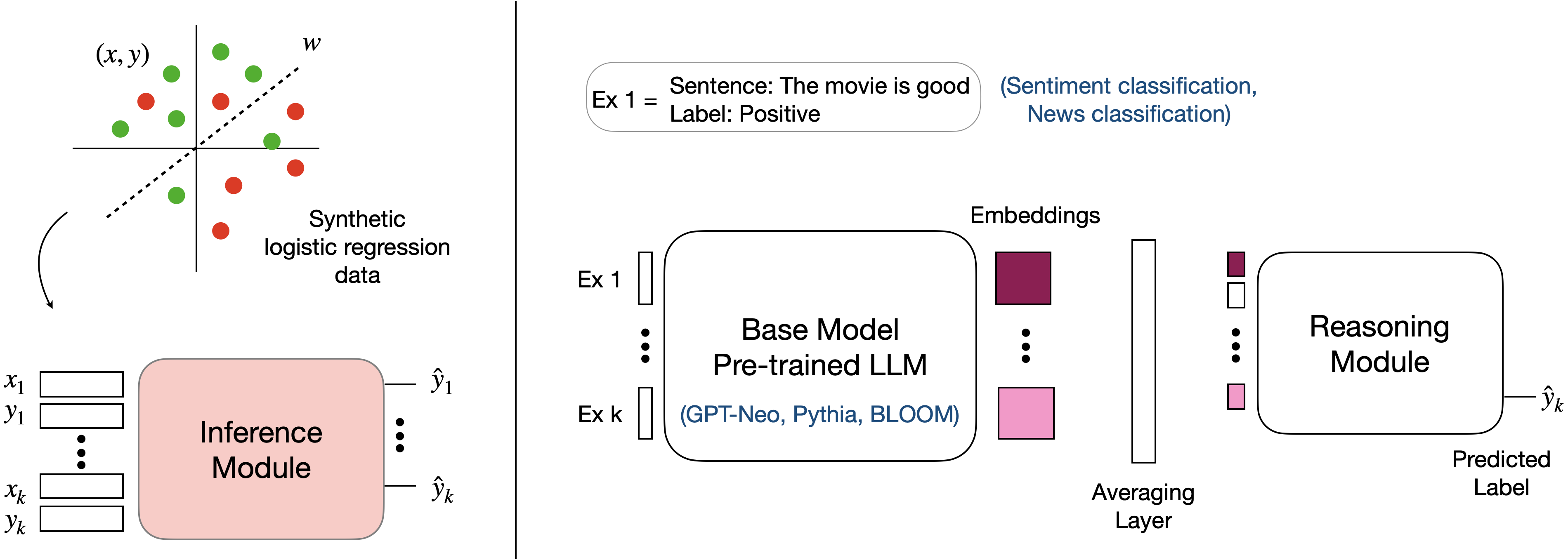
Figure 2: Tart. (Left) Inference module training procedure: The inference module is trained on sequences of synthetically generated logistic regression tasks. (Right) End-to-end framework: Tart composes a pre-trained LLM with the inference module. Tart uses the LLM to embed the input text. These embeddings, along with the train labels, are passed as a sequence to the inference module which generates a final prediction.

2 Related work

Prompt engineering focuses on improving the in-context task adaptation abilities of LLMs by modifying prompts. A line of work improves performance by carefully designing the natural language task specifications  [Aro+23, Wei+22a] while others improve performance by optimizing the examples chosen for the prompt [Dia+23, Liu+22a], encouraging the models to sequentially reason [Koj+22, Wei+22a, Zel+22] and aggregating prompts [Wan+22a, Wan+22]. Unfortunately, prompt-based task adaptation is noisy [Lu+22]. Alternatively, prompt tuning improves the in-context abilities of models by training a small amounts of learnable vectors [LL21, LAC21, Liu+22b] for specific tasks. While these methods have been shown to improve in-context learning performance, they require task-specific fine-tuning and are not task-agnostic.

Recent works seek to understand the in-context learning property of LLMs by presenting mechanistic interpretations of in-context learning [Osw+22], performing exploratory analysis of in-context learning behaviors [Wei+23], and explaining it as implicit Bayesian inference [Xie+21]. Existing literature demonstrates that LLMs can learn simple function classes in-context [Gar+22] and propose that LLMs are performing gradient descent when learning tasks in-context [Osw+22]. Complementary to these, our work provides insights on the mechanisms of in-context learning and its deficiencies. Furthermore, task transfer strategies adapt LLMs to a pre-specified target task. Strategies range from parameter efficient finetuning (PEFT) [Hou+19, Zha+23] to Low-Rank adaptation (LoRA) [Hu+22] which introduces trainable rank decomposition matrices into each layer to combining linear probing and fine-tuning [Kum+22]. While they have good performance, these methods require training models on a task-by-task basis in contrast to Tart.

3 Task adaptation strategies: Taxonomy and evaluation

We begin by describing the problem of adapting pre-trained language models for a collection of downstream tasks while being task-agnostic, competent in performance, and data-scalable. Given these criteria, we evaluate existing task adaptation approaches and propose a representation-reasoning decomposition to understand their relative performances.

3.1 Problem statement and evaluation criteria

Our focus is on methods for adapting pre-trained large language models (LLMs) for downstream tasks. Specifically, given an LLM and limited labeled data for a task, how does one adapt the model to the task? When evaluating a task adaptation strategy, we care about the following properties:

Task-agnostic.

Given the general capabilities of pre-trained LLMs, we strive to utilize the same model across different tasks without requiring any task-specific training. With the increase in model sizes, the cost of deploying task-specific models increase both during training (expensive hyper-parameter search) as well as during inference (deploying several models). In general, task-agnostic methods will scale better with increasing model sizes by side-stepping both these costs.

Performance quality.

We would like the adaptation approaches to be competitive in performance when compared with task-specific approaches across a wide range of tasks. For the binary classification tasks, the method should have accuracy comparable with task-specific approaches.

Data-scalable.

The task adaptation method should be scalable with the number of labeled task examples. In particular, the method should be capable of learning from large datasets, and continually improve its performance quality.

3.2 Taxonomy of task adaptation strategies

We can broadly taxonomize the existing task adaptation strategies for LLMs as in-context learning, fine-tuning the model, and training task-specific adapters (see Figure 1).

In-context learning.

In-context learning allows for adapting the model without updating any model parameters, by simply providing a few demonstrations of the task in the LLM prompt. In-context learning is completely task-agnostic since the same model can be used across tasks since no weights are updated at inference time. However, its performance is usually not at par when compared with task-specific methods and it does not scale well with data since the number of examples that can be utilized is bottlenecked by the context length of the model.

Fine-tuning.

This traditional class of methods update the model weights to adapt it specifically for the task, typically by performing gradient descent over the labeled dataset. Fine-tuning methods are not task-agnostic since they change the underlying model significantly but usually achieve state-of-the-art performance for any given task and are data scalable.

Adapters.

Adapters adapt the underlying LLM to a specific task by composing the LLM base model with an additional set of parameters which are optimized for the task. In contrast to fine-tuning which performs updates to the base model, adapters keep the base model frozen and only update the additional parameters. Performance of adapters is usually competitive with full fine-tuning.

3.3 Understanding performance via Representation-Reasoning decomposition

From the taxonomy of task adaptation approaches, only in-context learning satisfies the task-agnostic property but it consistently underperforms the task-specific tuning approaches. This section investigates why this performance gap exists. We hypothesize that it is either because (a) the representations learned by the LLM are insufficient to learn a good predictor for the specific task, or (b) the LLM lacks the capability to reason over these representations to make good predictions for the task.

To understand whether the representations have sufficient information, we train a task-specific linear classifier using these representations, also known as linear probing, and evaluate its accuracy. Let $\text{Acc}_{{\sf FT}}$, $\text{Acc}_{{\sf ICL}}$, and $\text{Acc}_{{\sf LR}}$ denote the accuracies obtained by fine-tuning, in-context learning, and by linear probing respectively. Using this as an intermediate, we decompose the performance gap

$$\Delta_{{\sf perf}}:\,=\text{Acc}_{{\sf FT}}-\text{Acc}_{{\sf ICL}}=\underbrace{\text{Acc}_{{\sf FT}}-\text{Acc}_{{\sf LR}}}_{\Delta_{{\sf rep}}}+\underbrace{\text{Acc}_{{\sf LR}}-\text{Acc}_{{\sf ICL}}}_{\Delta_{{\sf reas}}}$$ (1)

where $\Delta_{{\sf rep}}$ represents the gap in performance which can be attributed to insufficient representation capacity and $\Delta_{{\sf reas}}$ is the performance gap due to insufficient reasoning abilities. Using this decomposition, we consider the following hypotheses:

1. LLM representations have enough information to perform the task in-context, but they lack the reasoning abilities to perform the task well.

2. Fine-tuning affects both the representations and reasoning but the improvement in reasoning abilities primarily leads to better performance.

3. Fine-tuning and adapters are not task-agnostic because the task-specific training hurts their ability to transfer reasoning.

We now analyze each of the task adaptation approaches through the lens of the above hypotheses. We perform all experiments with three different classes of language models (GPT-Neo, Pythia, Bloom) across a collection of 6 binary classification tasks. See Appendix B for further details.

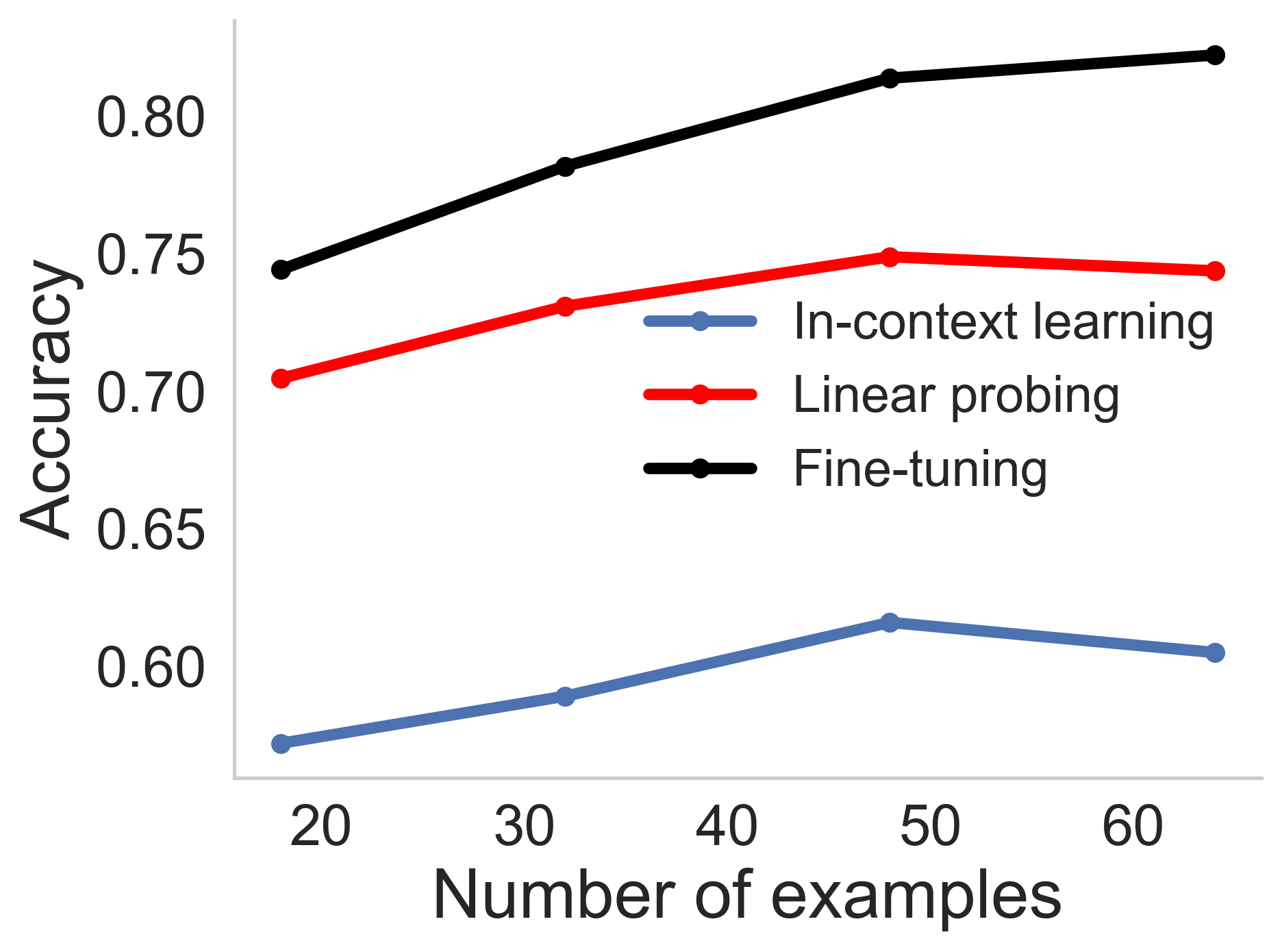
(a)

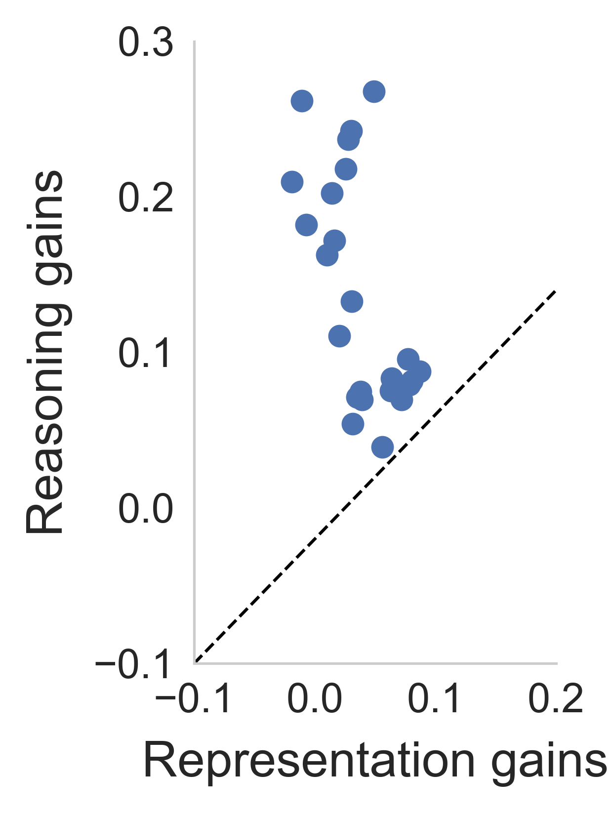
(b)

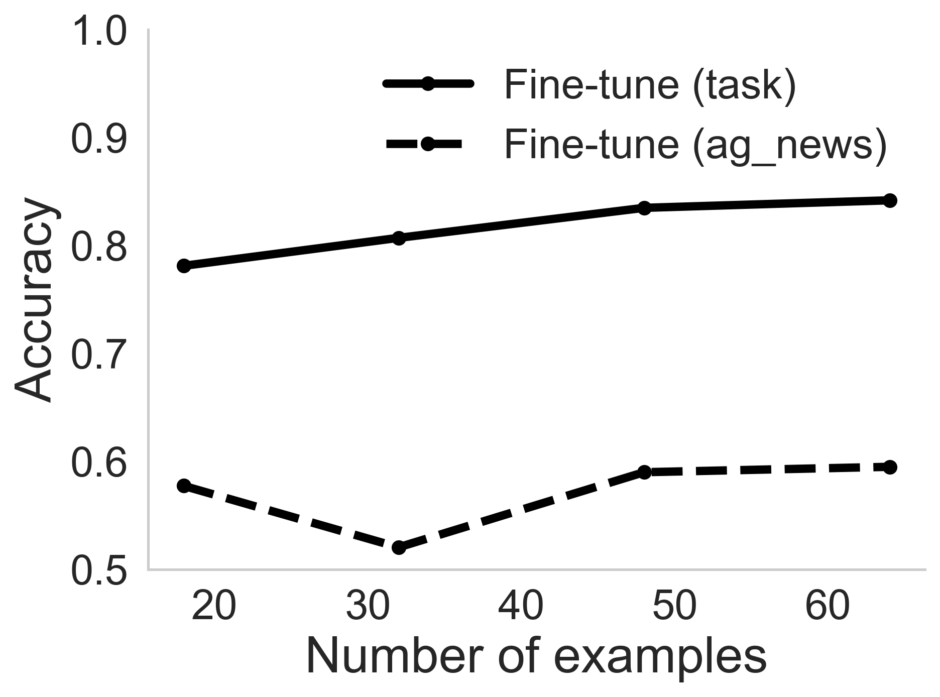
(c)

Figure 3: All results for GPT-Neo (125M). (a) Accuracy of in-context learning vs. linear probing on model embeddings: representations have sufficient information. (b) Scatter plot showing the representation and reasoning gains (see eq. (1)) across different NLP datasets for a fine-tuned model when compared to base in-context learning. Fine-tuning majorly improves task-specific reasoning across datasets. (c) Accuracy (averaged across $6$ datasets) of model fine-tuned on AGNews and tested on a separate task X vs model fine-tuned on task X and tested on the same task X. On average, fine-tuning hurts task-agnosticity can can be up to $25\%$ off from fine-tuning for the specific task.

In-context learning: LLMs lack reasoning abilities.

We begin by studying the representation and reasoning gaps, as defined in eq. (1), for in-context learning. In Figure 3(a), we plot the average accuracy across datasets for in-context learning, task-specific fine-tuning, and linear probing. We see that across models and different numbers of in-context examples, the reasoning gap $\Delta_{{\sf reas}}$ accounts for up to $79.11$% of the performance gap between in-context learning and fine-tuning. This indicates that the LLM representations have sufficient information but lack the ability to reason over them.

Fine-tuning: Improves task-specific reasoning.

We next investigate how fine-tuning for a specific task affects the performance of the base model. In Figure 3(b), we show a scatter plot of the gains that can be attributed to improved representations against the reasoning gains. We see that, across models, reasoning improvements accounts for $73.06$% of the improvements. This indicates that while fine-tuning improves both reasoning and representations of the LLM, the gains are predominantly due to improvements in task-specific reasoning. Furthermore, this task-specific fine-tuning of the LLM hurts its performance on other tasks. In Figure 3(c), we show that the accuracy of a model fine-tuned on the AGNews dataset [ZZL15], leads to an average decrease of $25.77$% on other tasks. Furthermore, this drop in accuracy can be attributed to the drop in task-specific reasoning capabilities—these account for $72.58$% of the drop (see Appendix B for more details).

Adapters: Impairs task-agnosticity via reasoning.

Task-specific adapters do not change the underlying representation ability of the model. To study their ability to generalize across tasks, we train an adapter for the AGNews dataset and evaluate it on other tasks. In Appendix B, we show that the performance drops across tasks by an average of $19.8$%, indicating that adapters only learn task-specific reasoning abilities.

4 Tart: Task-Agnostic Reasoning Transformers

The above analysis showed how it is the effective reasoning capabilities of the LLMs which limits its performance when compared with task-specific adaptation approaches. Building on this insight, we propose Tart, which learns a general-purpose reasoning module completely agnostic to the underlying base LLM and when composed with any LLM via its embeddings, generically improves upon its reasoning abilities. Tart is a completely task-agnostic method which works across a suite of tasks without any task-specific training.

Tart comprises of two components: a generic task-agnostic reasoning module, and embeddings from the base LLM. The reasoning module is trained using only synthetic data (Gaussian logistic regression problems), agnostic of the auto-regressively trained language model, with the objective of learning to perform probabilistic inference (Section 4.1). This learned transformer module is then composed with the base LLM, without any training, by simply aggregating the output embedding and using those as an input along with the class label (Section 4.2). Together, these components make Tart task-agnostic, boost performance quality by improving reasoning, and make the approach data-scalable by aggregating input embeddings into a single vector.

Intuitively, the Gaussian logistic regression task is a simple probabilistic reasoning task wherein the objective is to regress a given feature vector to a discrete binary label. Teaching an independent module to perform a family of these tasks and composing them with pre-trained language models can be seen as a way to generically improve upon the LLM’s reasoning abilities by making them perform such regression better.

4.1 Reasoning module: Can Transformers learn probabilistic inference?

Tart’s reasoning module is a Transformer-based model which is trained to perform probabilistic inference in-context using only synthetically generated data.

4.1.1 Training the reasoning module

The reasoning module is a Transformer model which is auto-regressively trained on a family of logistic regression tasks, with each input sequence corresponding to a different logistic regression problem. We next describe the model architecture and the training procedure.

Model architecture.

The reasoning module is based on the standard decoder-only Transformer architecture from the GPT-2 family (see Appendix C.1 for details). The architecture takes as input a sequence of vectors and is trained to predict the next vector in the sequence. The input sequence consists of $k$ pairs of labeled examples $(x_{1},y_{1}),(x_{2},y_{2}),\ldots,(x_{k},y_{k})$, with each example $z_{i}=(x_{i},y_{i})$ using only two input positions of the transformer – one for the covariates $x$ and the other for the label $y$. This is in contrast to standard LLMs where each example is spread over multiple tokens which limits how many examples can be put in the context. For example, with a context window of 2048, our module can support 1024 examples while the base model can support only 10 examples, assuming each demonstration comprises 200 natural language tokens.

Training procedure.

This module is trained using gradient descent to minimize the population loss

$$\ell(T_{\theta}):\,=\mathbb{E}_{x,y}\left[\frac{1}{k}\sum_{i=1}^{k}\ell_{{\sf CE}}(T_{\theta}(z_{1:i-1},x_{i}),y_{i})\right]\;,$$ (2)

where $z_{1:i-1}$ corresponds to the first $i-1$ examples and $\ell_{{\sf CE}}$ is the cross-entropy loss evaluated on the transformer prediction and the true $y_{i}$. Each training sequence $s_{t}$ used to update the parameters $w$ comprises a different $d$-dimensional logistic regression problem, sampled as

$$\text{Sequence }s_{t}:w_{t}\sim\mathcal{N}(0,I_{d}),\quad x_{i,t}\sim\mathcal{N}(0,I_{d}),\quad y_{i,t}\sim\sigma(\alpha\langle x_{i,t},w_{t}\rangle)\qquad\text{for }i\in[k]\;,$$ (3)

where $\sigma$ represents the sigmoid function and the multiplier $\alpha$ determines the noise level of the problem. We train our model with $d=16$ and $k=256$. Observe that the loss is only computed on the predicted output of the features $x$ in the sequence. We describe the model hyper-parameters and the training procedure in more detail in Appendix C.1.

We trained the reasoning module with input dimension set to 16 with the labels $y$ encoded in this space using a one-hot encoding by appending the true label with zeros. While most base models produce representations which are much higher dimensional (ranging from 784 to 2048). In order to reduce the dimensionality of these representations, we perform PCA on the output embeddings of the base model, learning the components using only the training points available for that specific task. The test examples are then projected onto these principal components to produce 16 dimensional input representations.

4.1.2 Properties of reasoning module

The task-agnostic reasoning module described above is trained to perform well on a family of logistic regression tasks. We study some properties of the reasoning module, in particular how well it learns to perform the task at an instance level and how robust is it to variations in the noise level $\alpha$.

Accuracy of probabilistic inference.

For understanding the instance level performance of our reasoning module, we evaluate it on a sample of $64$ different logistic regression problems, sampled according to eq. (3). For each problem, we train task-specific linear classifiers using logistic regression and compare them with our task-agnostic reasoning module. In Figure 4(a) we plot the deviation of the predicted probabilities (averaged over the $64$ problems) from the true probabilities for our reasoning module and the task-specific logistic solvers as a function of the number of examples used for predictions. We observe that the error for our reasoning module decreases as a function of the number of in-context examples and is within $2\%$ of the task-specific logistic function.

Robustness to noise level.

We study the robustness of the learned module to the noise levels, $\alpha$, of the logistic regression problem. Recall that we trained our inference module by fixing the noise level $\alpha=10$. At inference time, we vary the noise level to $[0.5,1,10,20]$, where lower values corresponds to noisier problem. The reasoning module generalizes to easier problem without any drop in accuracy but as we make the problem harder $(\alpha=[0.5,1])$, the error increases progressively (see Figure 4(b)).

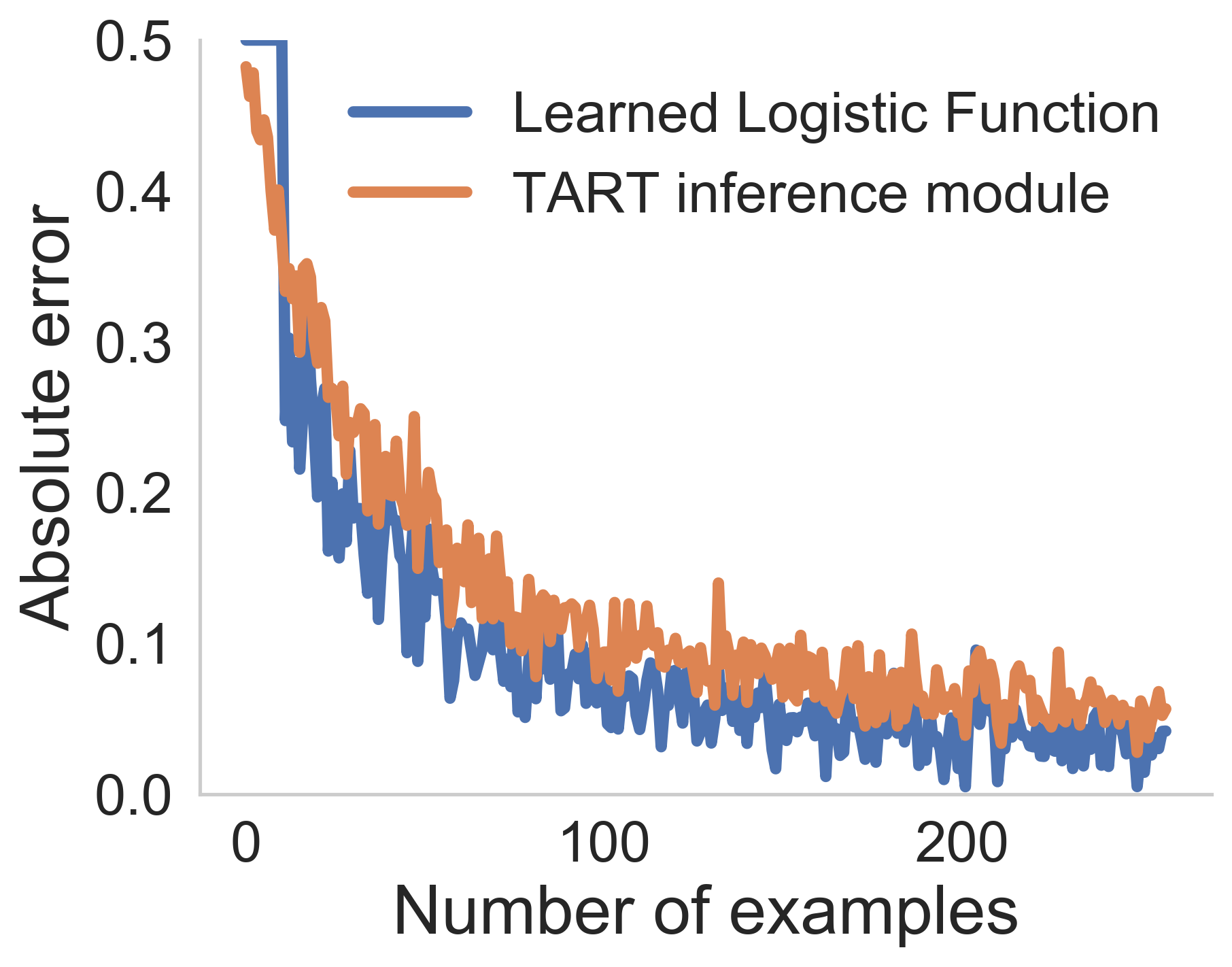
(a)

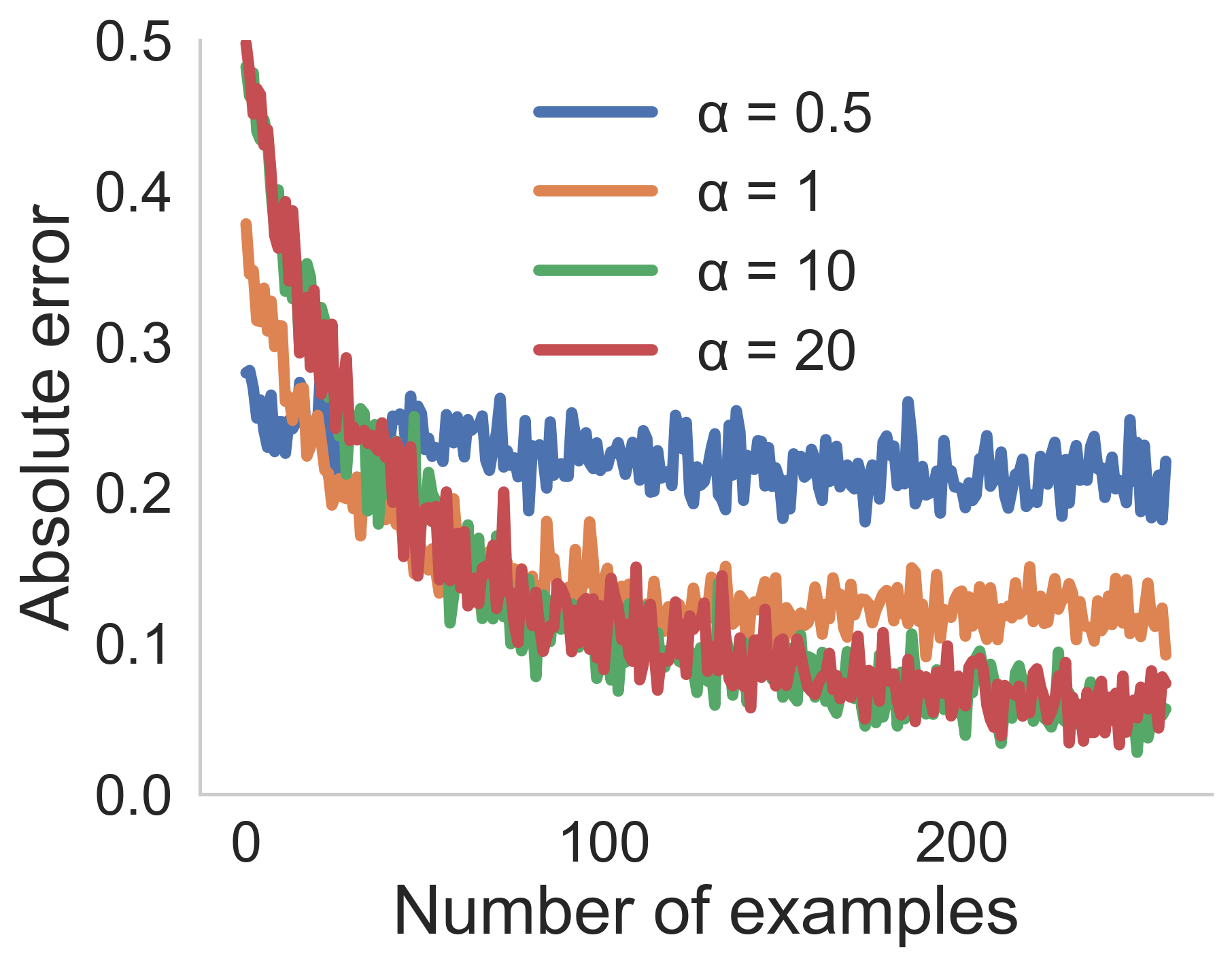
(b)

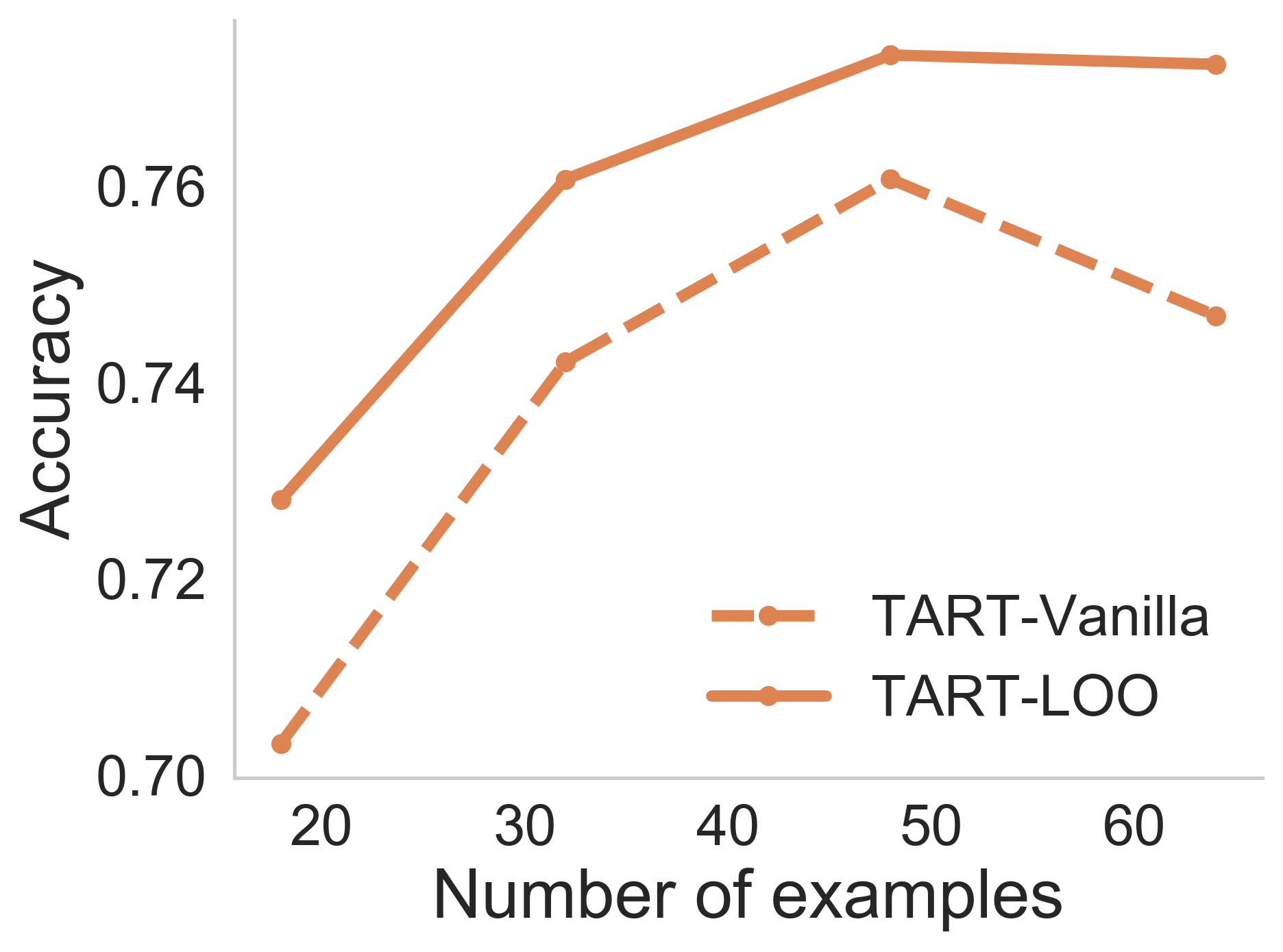
(c)

Figure 4: Properties of Tart’s inference module. (a) Comparison with learned logistic function: inference module recovers underlying probabilities. (b) Variation in error with different noise levels for model trained on $\alpha=10$. (c) Comparison of Tart performance when using LOO embeddings and vanilla embeddings.

4.2 Role of representations: Which embeddings to take?

The reasoning module composes with a base LLM through its final layer embeddings. A natural way to produce these embeddings is to place all the train examples in-context and then average the embedding vectors corresponding to the particular example (see Figure 5(a)). At inference time, we append the test example to the training set, and average the embeddings corresponding to this example. We call these vanilla embeddings. Our experiments reveal that these embeddings seem to saturate (or even hurt performance) beyond a certain number of in-context examples (see Figure 4(c)). One reason can be that the causal nature of the model causes these embeddings to have asymmetric information—the embeddings of each example is influenced by its preceding examples.

To counter this asymmetry, we propose leave-one-out (LOO) embeddings where the embeddings for each training point is formed by placing all the other train examples before it in the prompt such that all the embedding are formed with the same information content (see Figure 5(b)). In Figure 4(c), changing the embedding style from vanilla to LOO consistently improves performance across models and tasks. The LOO-embeddings help Tart be data-scalable by enabling it to embed a much larger number of points than the context window can support. To do so, we use only a subset of the train examples as the in-context prompt. The reasoning module, by its architecture design, can already accommodate many more examples than supported by the context window of the base LLM.

(a) Vanilla Embeddings

(b) LOO Embeddings

Figure 5: Tart Embedding Protocols. (a) For the vanilla embeddings, the test example is appended to the training set and the sequence is passed to the base model. The representation for each train example in this sequence is taken as the average embedding across all its tokens. (b) For the LOO embeddings, we generate embeddings for each train example separately by placing all the other train examples before it in the prompt and averaging the embeddings over the final example’s tokens. The figure shows how to compute the embedding for the $i^{\text{th}}$ training example.

4.3 Theoretical analysis: Generalization of Tart to language tasks

We study the generalization properties of the proposed task-agnostic method Tart. Note that that the inference module is trained completely on synthetic data while at evaluation time, our input is the embeddings from a natural language task. In Theorem 1 we show that its performance on the natural language task depends on the distribution shift from the synthetic to the true distribution (see Appendix C.3 for a formal statement and proof).

Theorem 1 (Informal).

Let $\mathcal{T}$ represent the class of transformer models and $T_{S}\in\mathcal{T}$ denote the trained reasoning module on set $S$ of synthetic regression with $n_{{\sf syn}}$ sequences sampled from distribution $P_{{\sf syn}}$ in eq. (3). The error of the transformer $T_{S}$ when evaluated on a distribution $P_{{\sf NL}}$ over natural language sequences is

$${\sf err}_{P_{{\sf NL}}}\lesssim W_{1}(P_{{\sf NL}},P_{{\sf syn}})+\sqrt{\frac{\text{Comp}(\mathcal{T})}{n_{{\sf syn}}}}+\hat{{\sf err}}_{P_{{\sf syn}}}(T_{S})\;,$$ (4)

where $W_{1}$ denotes the Wasserstein-1 metric, $\text{Comp}(\mathcal{T})$ represents the complexity of class $\mathcal{T}$, and $\hat{{\sf err}}$ represents the error on the empirical distribution.

A few comments are in order: The first term represents the distribution shift error between the true natural language task and the synthetic task. The second term corresponds to the generalization error on the logistic regression task, which can be made arbitrarily small since it scales with $n_{{\sf syn}}$, the number of synthetic datapoints which can be generated without any cost. The third term is the optimization error indicating how well has the reasoning module $T_{S}$ fit to the synthetic training set.

5 Experimental evaluation

We evaluate Tart on a wide range of binary classification tasks across three domains: language, vision and audio. We demonstrate that Tart improves base in-context performance and closes the gap with standard task-specific strategies. We also conduct ablations to demonstrate that Tart scales with model size and can support 10x more samples than in-context learning.

5.1 Experimental setup

Datasets.

We briefly describe the datasets used, with details available in Appendix D.1. We consider $14$ different binary classification tasks ranging from sentiment classification, news article categorization to spam detection. The evaluation datasets include: SST [Soc+13], Rotten Tomatoes [PLV02], SMS Spam [AHY11], IMDB [Maa+11], Civil Comments [Bor+19], AGNews [ZZL15], DBPedia [ZZL15], and the Youtube dataset [Zha+21]. Since AGNews and DBPedia14 are multi-class datasets, we construct 4 binary classification tasks from each dataset respectively. For each dataset, we truncate the input text to be at most 100 characters to enable us to fit sufficient number of samples in-context.

Model families.

We evaluate our method across three different families of models: GPT-Neo [Bla+21], Pythia [Bid+23], and Bloom [Sca+22]. For our evaluations across 14 datasets, we use GPT-Neo (125M), Pythia (160M) and Bloom (560M). For ablations on larger models, we evaluate models with 1B parameters across each of the model families (i.e., GPT-Neo (1.3B), Pythia (1.4B) and Bloom (1.7B)) and models with 3B parameters (i.e., GPT-Neo (2.7B), Pythia (2.8B) and Bloom (3B)). We additionally evaluate on GPT-J (6B) [WK21].

Baselines.

We evaluate our models against all types of task-adaptation strategies described in Section 3.2: 1) in-context learning, 2) full fine-tuning, 3) last layer fine-tuning, 4) LM head fine-tuning, and 5) adapters. For each baseline, we perform an extensive hyper-parameter search over number of epochs and learning rate for each dataset in order to optimize performance (see Appendix D.1 for hyperparameter details). For Tart, we chose a base default set of parameters and use the same inference module with the exact same weights for all the experiments in this section.

5.2 Natual language benchmark evaluations

For this section, all reported accuracies are averaged over $5$ independent random seeds. A complete set of results with standard deviations can be found in Appendix D.2.

Performance with respect to baselines.

As shown in Appendix D.2, averaged across all tasks and model families, Tart improves upon the base in-context learning performance by an average of $18.4$ points, improves upon adapter heads by $3.4$ points, and is within $3.1$ points of full fine-tuning. We also observe that Tart consistently outperforms the task specific strategies of LM head fine-tuning and last layer fine-tuning.

Model	Tart	GPT-J (6B)	OPT (175B)	Bloom (176B)	GPT-3 (175B)
Accuracy	0.634	0.608	0.637	0.595	0.673

Table 1: RAFT (HELM) Binary Classification Performance (Average Accuracy). Tart is used with GPT-Neo (125M) model which is $1000$x smaller than the corresponding 175B parameter models. Tart outperforms Bloom (176B) and is competitive with OPT (175B) and GPT-3 (175B).

Performance on RAFT Benchmark

We evaluate Tart on all binary classification tasks in the RAFT Benchmark, following the protocol used in HELM [Lia+22]. When applied with GPT-Neo (125M), Tart outperforms Bloom (176B), and is within $4\%$ points of GPT-3 (175B), both of which are $1000$x larger in size. See Table 1 for exact accuracies.

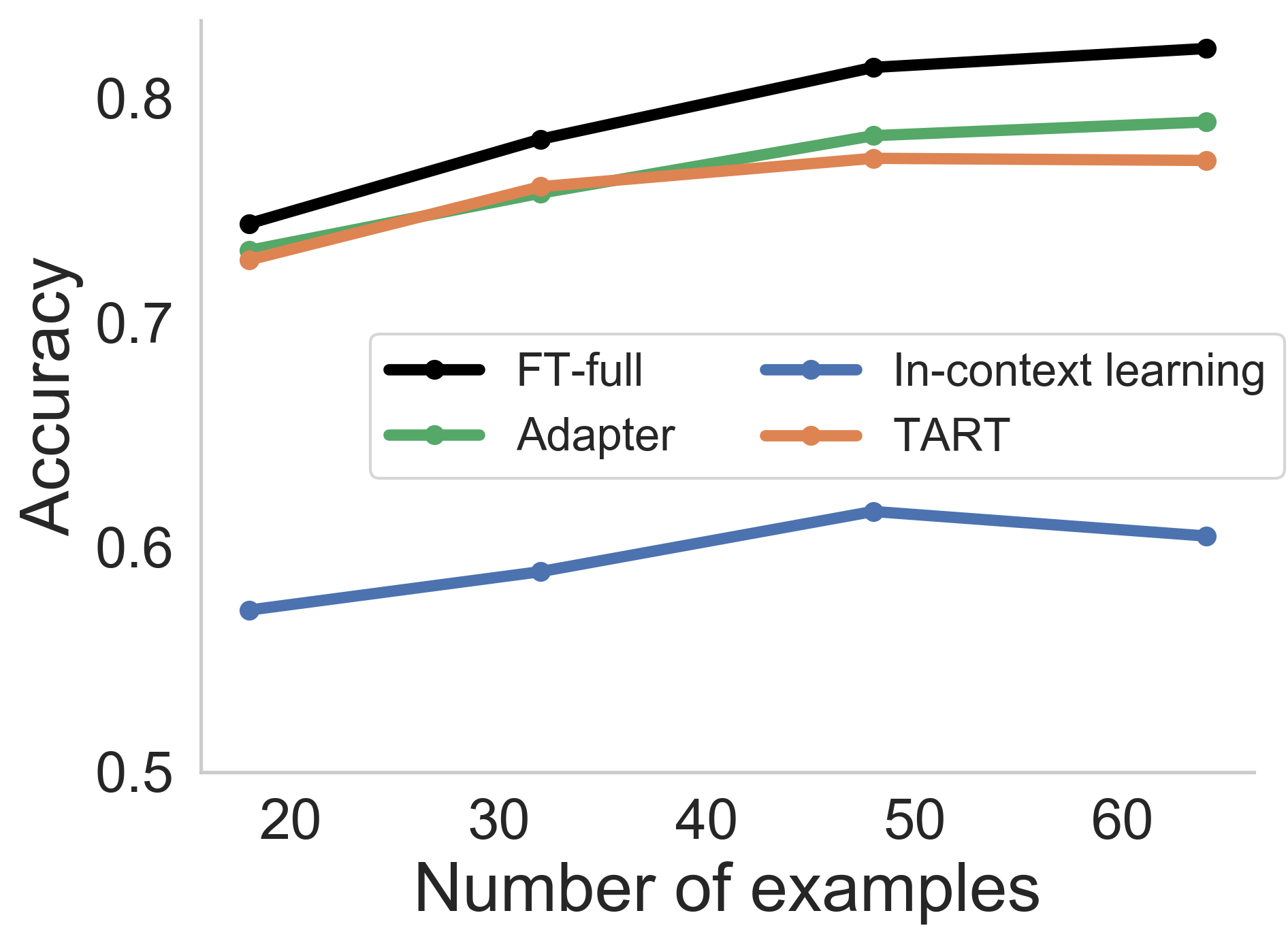
(a)

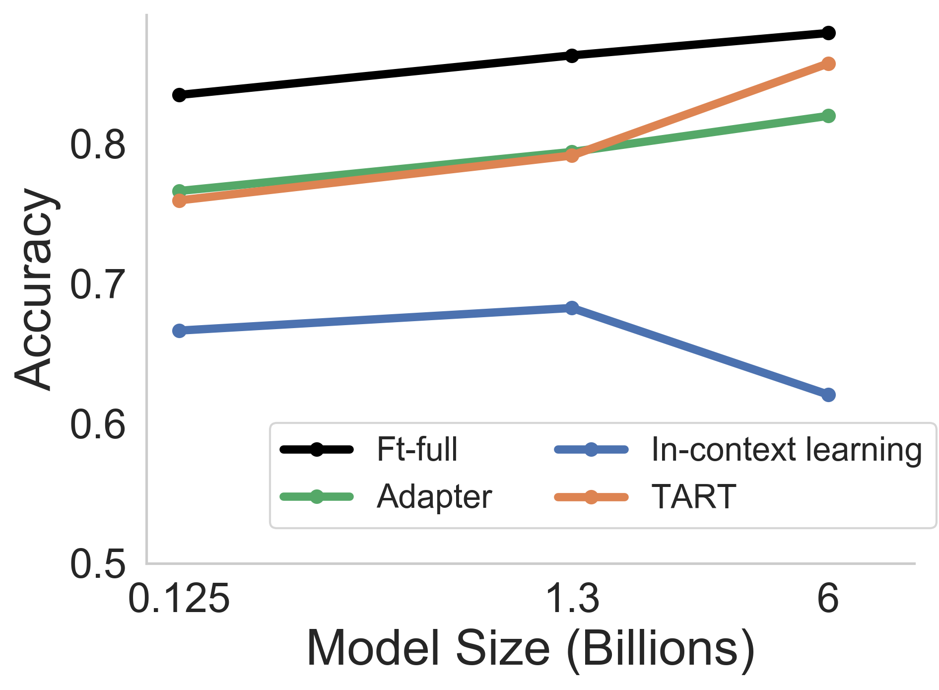
(b)

(c)

Figure 6: Effects of scale. (a) Effect of number of in-context examples on performance for different task adaptation strategies. (b) Effect of model size on the performance of different task adaptation strategies. (c) Beyond context length limitations, performance comparison with respect to number of in-context examples.

Performance with number of in-context examples.

Our results demonstrate that performance of Tart scales with number of in-context examples (see Figure 6(a)). Across $14$ tasks and $3$ model families, when scaling from $18$ to $64$ examples, Tart improves performance by an average of $4.8$%. Correspondingly, full fine-tuning improves performance by $9.0$%.

Scaling with base model size.

We analyze how different task-adaptation strategies scale with respect to model size using the GPT-Neo family: GPT-Neo (125M), GPT-Neo (1.3B) and GPT-J (6B). Figure 6(b) shows that when scaling from 100M to 6B parameters, performance of task-specific methods and Tart increases as a function scale. For Tart, the performance increases by $9.8\%$ while using the same inference module across model sizes. Furthermore, the difference in performance between Tart and fine-tuning baseline reduces from $7.5\%$ to $2.2\%$ from the 100M scale to 6B scale.

Beyond context length.

We evaluate the data-scaling properties for both in-context learning and Tart (Figure 6(c)). To demonstrate the scaling property, we do not truncate the input text to $100$ characters and utilize the entire text sequences. For Tart, we observe that accuracy continues to improve when scaling from $18$ to $256$ in-context examples with $6.8$% lift in performance. In comparison, ICL, which is bottlenecked by context length, supports $10$x less samples, with the context window saturating at $24$ examples only and lags Tart by an average of $19.1$%.

5.3 Extensions to other modalities

(a) MNIST

(b) CIFAR-10

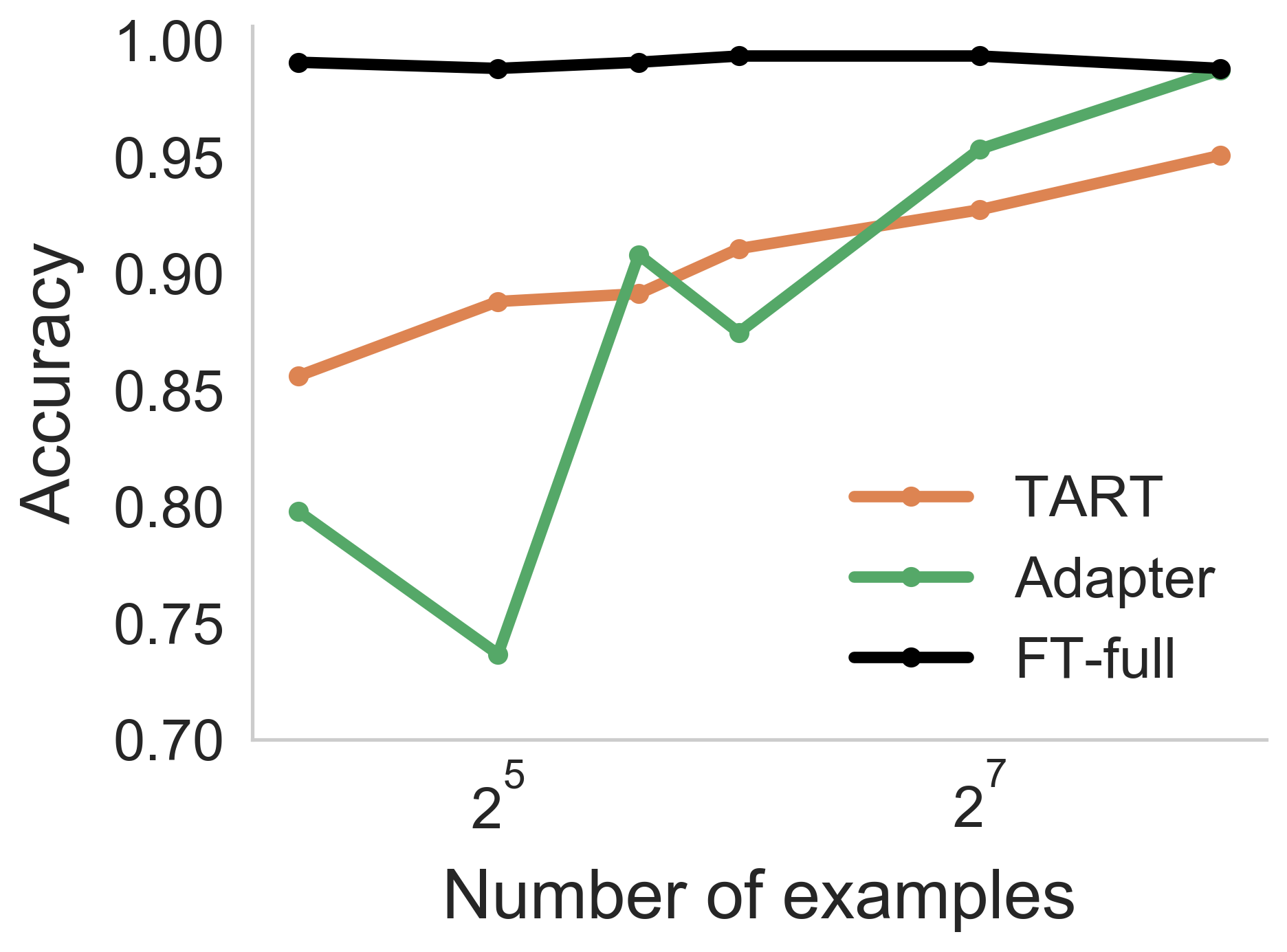
(c) Speech Commands

Figure 7: Tart can generalize across domains using the same inference module that was used for language benchmarks: Performance across vision tasks (MNIST, CIFAR-10) and an audio task (Speech Commands).

We demonstrate that Tart is not only agnostic to models and tasks, but also modalities. We extend Tart to classification tasks on modalities beyond language: vision and audio. For vision tasks, we use representations from Google’s 307M parameter pretrained Vision Transformer (ViT) model [Wu+20]: ViT-large-patch16-224-in21k. For audio tasks, we use representations from OpenAI’s 1.5B parameter pretrained Whisper model [Rad+22]: Whisper-large. In applying Tart to the representations from these models, we provide a way for performing in-context learning in modalities beyond text. We refer the reader to Appendix D.3 for further details on the experiment setup.

Vision application.

We evaluate the performance of Tart on binary classification versions of CIFAR-10 [Kri09] (classes plane and bird) and MNIST [LCB10] (classes 0 and 8). As shown in Figure 7(a) and 7(b), performance of Tart is competitive with task-specific adaptation approaches.

Audio application.

We evaluate Tart on a binary classification version of the Speech Commands dataset [War18], where the task is to classify “stop” and “go” utterances. As shown in Figure 7(c), performance of Tart is competitive with task-adaptation approaches.

6 Discussion

We look at the problem of task-agnostic learning with LLMs. We show that LLMs lack the ability to perform simple reasoning over their learned representations and introduce Tart, a task, model and domain agnostic method for improving their reasoning abilities. In this work, we focus on binary classification tasks, showing that synthetic, logistic regression task data can be used to train a generic reasoning module capable of completing this class of tasks. Extensions to multi-class classification tasks are possible either using a one-vs-all approach or by training Tart’s reasoning module using multi-class synthetic data. In future work, we seek to understand whether synthetic tasks exist for training other generic reasoning modules, capable of improving base LLM performance on tasks such as generation or summarization.

Acknowledgements

We are grateful to Simran Arora, Rishi Bommasani, Niladri Chatterji, Arjun Desai, Sabri Eyuboglu, Neha Gupta, Karan Goel, Erik Jones, Ananya Kumar, Cassidy Laidlaw, Megan Leszczynski, Piero Molino, Laurel Orr, Michael Poli, Dimitris Tsipras, Michael Wornow, Ce Zhang, and Michael Zhang for their helpful comments and feedback, and discussions which helped shape this project.

We gratefully acknowledge the support of NIH under No. U54EB020405 (Mobilize), NSF under Nos. CCF1763315 (Beyond Sparsity), CCF1563078 (Volume to Velocity), and 1937301 (RTML); US DEVCOM ARL under No. W911NF-21-2-0251 (Interactive Human-AI Teaming); ONR under No. N000141712266 (Unifying Weak Supervision); ONR N00014-20-1-2480: Understanding and Applying Non-Euclidean Geometry in Machine Learning; N000142012275 (NEPTUNE); NXP, Xilinx, LETI-CEA, Intel, IBM, Microsoft, NEC, Toshiba, TSMC, ARM, Hitachi, BASF, Accenture, Ericsson, Qualcomm, Analog Devices, Google Cloud, Salesforce, Total, the HAI-GCP Cloud Credits for Research program, the Stanford Data Science Initiative (SDSI), and members of the Stanford DAWN project: Facebook, Google, and VMWare. CDS was supported by a NSF CAREER (award 2046760).

The U.S. Government is authorized to reproduce and distribute reprints for Governmental purposes notwithstanding any copyright notation thereon. Any opinions, findings, and conclusions or recommendations expressed in this material are those of the authors and do not necessarily reflect the views, policies, or endorsements, either expressed or implied, of NIH, ONR, or the U.S. Government.

Appendix A Fine-tuning model with NL-based Probabilistic Inference Tasks

As highlighted in Section 1, we describe the details for directly fine-tuning an LLM on synthetically generated probabilistic inference tasks to improve reasoning capabilities. For the following experiments, we use GPT-Neo (125M) as the base model.

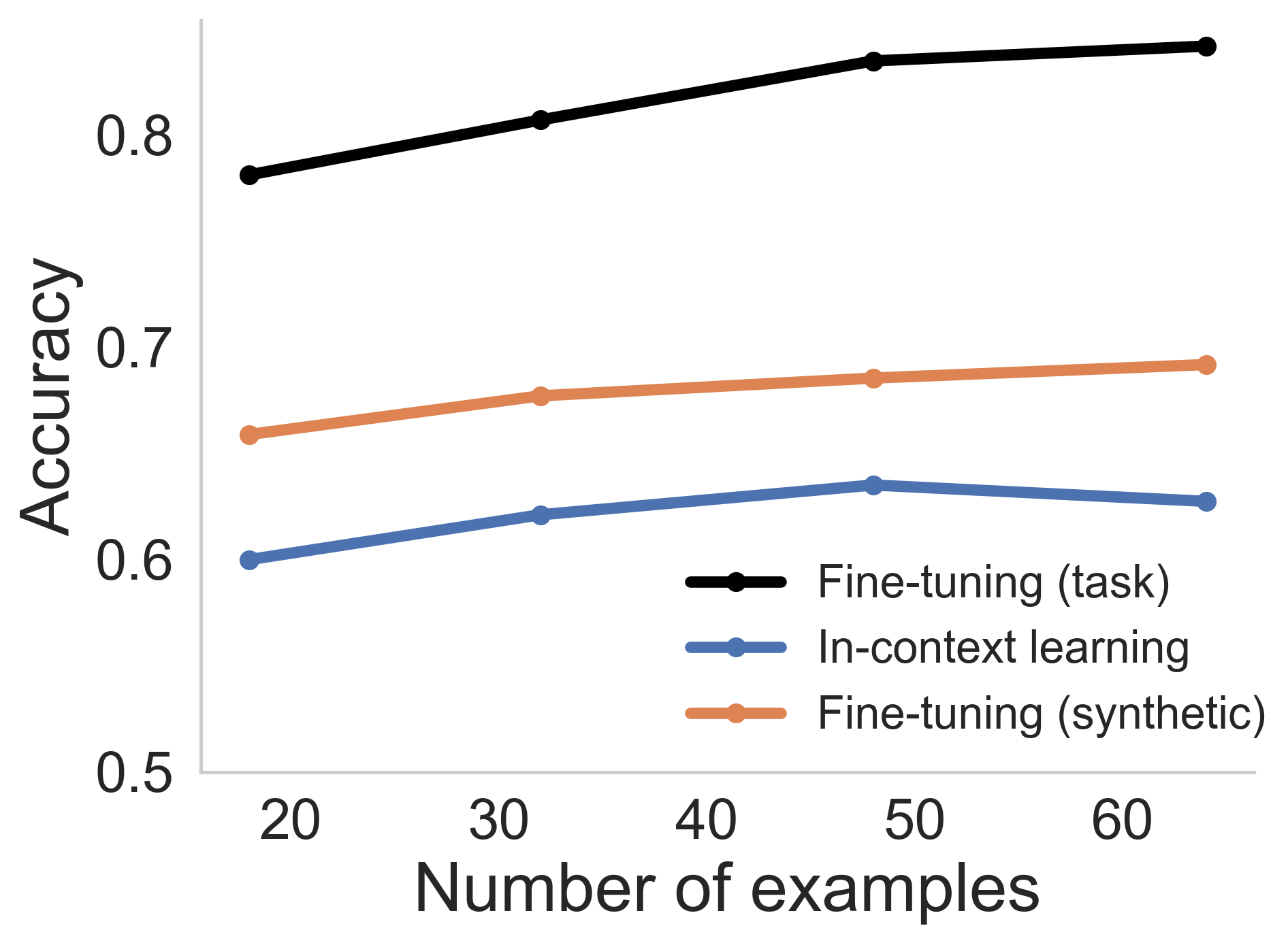
(a)

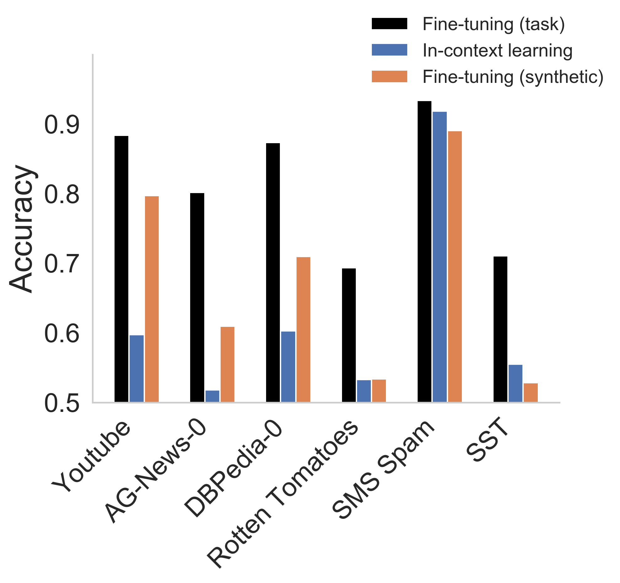
(b)

Figure 8: Fine-tuning with NL synthetic task. (Left) Averaged over 6 different tasks, fine-tuning with the NL synthetic task provides a lift over base in-context learning, and scales with number of examples. (Right) Dataset level comparisons between task-specific fine-tuning, in-context learning and synthetic fine-tuning: synthetic fine-tuning outperforms base in-context learning on 4 out of 6 datasets, but lags task-specific tuning.

A.1 Training Task

We fine-tune the base model using a sequence of $k$ pairs of synthetically generated labeled natural language examples $(x,y)$. Each example $x$ in the sequence $s=(x_{1},y_{1}),\ldots,(x_{k},y_{k})$ consists of a list of strings constructed from a fixed $V$ size of dimension $d=30$ . We use the following fixed vocabulary: [ “sports”, “love”, “hate”, “car”, “school”, “family”, “work”, “sleep”, “water”, “tree”, “fox”, “train”, “random”, “movie”, “music”, “book”, “play”, “house”, “spell”, “bar”, “jump”, “park”, “run”, “hill”, “fast”, “slow”, “talk”, “wallet”, “orange”, “apple”, “ball”, “cat” ].

To generate a particular example $x_{i}$, we sample each coordinate $x_{i,j}$ uniformly from the set $\{-1,+1\}$. If the sampled value is $+1$, we set the value to be the corresponding word in the vocabulary, that is, $x_{i,j}=V_{j}$. Otherwise, the word $x_{i,j}$ is set to “null”. For a given sequence $s$, we generate each of the labels $\{y_{i}\}$ as:

$$w_{t}\sim\mathcal{N}(0,I_{d}),\quad y_{i}\sim\sigma(\alpha\langle x_{i},w\rangle),\text{for }i\in[k]\;,$$ (5)

where we set noise parameter $\alpha=5$. If the sampled output is 0, we set the $y_{i}$ to “negative” and “positive” otherwise.

Finally, the inputs are formatted with following template: “$x_{1}$ : $y_{1}$ , $x_{2}$ : $y_{2}$ , … , $x_{k}$ : $y_{k}$” and the model is trained using gradient descent on the loss

$$\ell(T_{\theta}):\,=\mathbb{E}_{x,y}\left[\frac{1}{k}\sum_{i=1}^{k}\ell_{{\sf CE}}(T_{\theta}(z_{1:i-1},x_{i}),y_{i})\right]\;,$$ (6)

where $z_{1:i-1}$ corresponds to the first $i-1$ examples and $\ell_{{\sf CE}}$ is the cross-entropy loss evaluated on the transformer prediction and the true $y_{i}$.

More concretely, a sample input sample sequence $s$ to be used for training looks like:

"sports love null car ... cat: positive,
null love null car ... null: negative,
...
sports null hat null ... cat : positive"

A.2 Training Parameters

We train GPT-Neo (125M) on this synthetic task with a learning rate of 0.0001 and a batch size of 4. For each sequence we sampled a total of $k=60$ examples and trained the model for 10000 steps.

A.3 Evaluation

We evaluate on 6 datasets: AG News [ZZL15], DBPedia [ZZL15], SST [Soc+13], SMS Spam [AHY11], Youtube [Zha+21] and Rotten Tomatoes [PLV02]. We truncate the input texts to 100 characters to fit more in-context examples. We evaluate over a range of context sizes ($k$=[18, 32, 48, 60]). At evaluation time, we use the same “sentence : label” format that was used to train the model. We evaluate over 3 random seeds. In Figure 8, we compare the performance of the model fine-tuned on probabilistic inference tasks and the base in-context learning performance. While the performance of the fine-tuned model is better than the base in-context learning capabilities, task-specific fine-tuning still outperforms it by an average of $16.87\%$ (see Figure 8).

Appendix B Details for Representation-Reasoning decomposition evaluations

In this section, we provide details for the experimental evaluation and additional results for the representation-reasoning decomposition introduced in Section 3.3.

B.1 Experimental setup

For these experiments, we evaluate three different language models: GPT-Neo (125M), Pythia (160M), and Bloom (560M) on a collection of 6 binary classification datasets: AG News [ZZL15], DBPedia [ZZL15], SST [Soc+13], SMS Spam [AHY11], Youtube [Zha+21] and Rotten Tomatoes [PLV02]. For each model, we run evaluations for three different random seeds, where the randomness was in the set of datapoints chosen for the training task. For the hyperparameters, we performed an extensive search for all models across datasets. For details on these hyperparameters and the adapter architecture we evaluate over, see Appendix D.1.

To conduct linear probing over the embeddings, we perform logistic regression over the output embeddings of each model and the given labels in the training set using the built-in logistic regression solver from the scikit-learn python library, utilizing the lbgfs solver.

B.2 Detailed results

For each class of methods in the task-adaptation taxonomy from Section 3.2, we now describe the details of the experimental evaluation and present additional results.

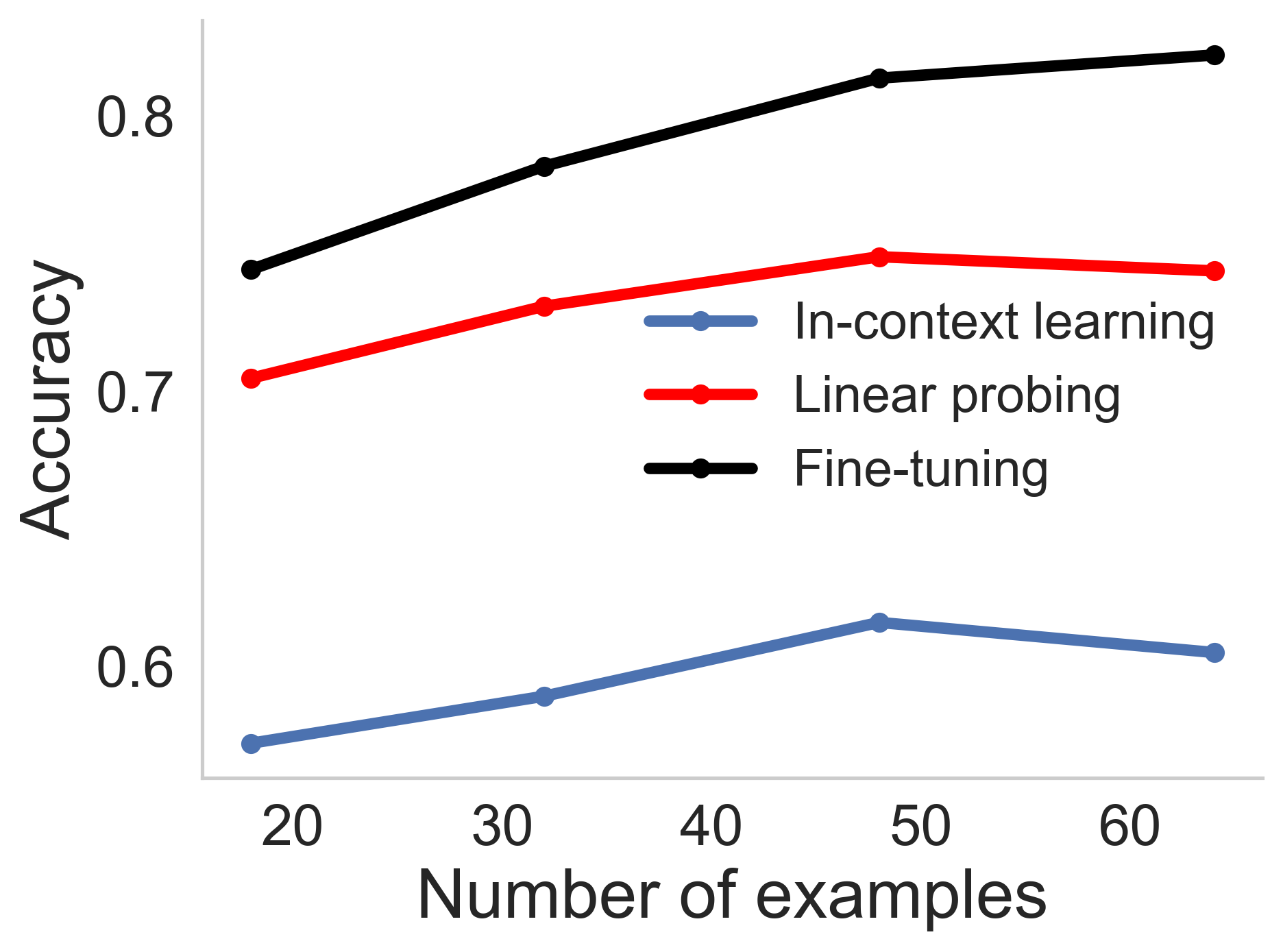
(a) GPT-Neo (125M)

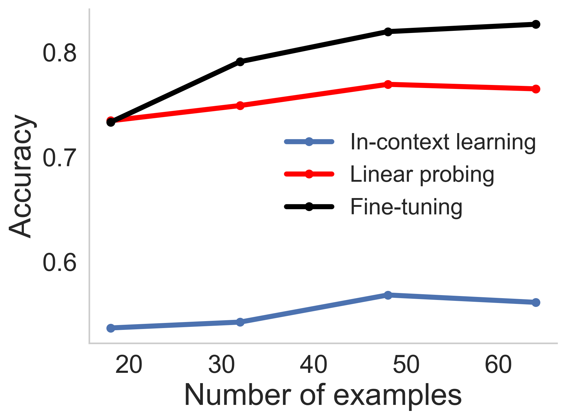
(b) Pythia (160M)

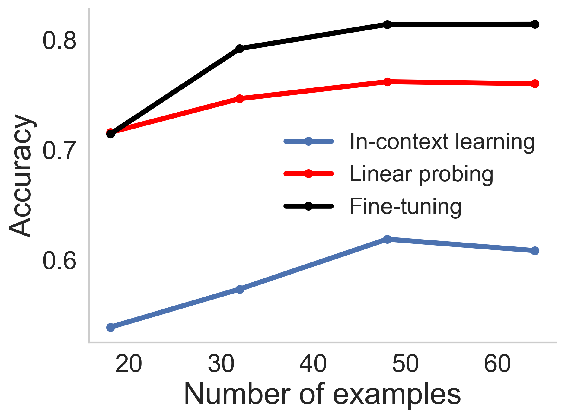
(c) Bloom (560M)

Figure 9: Comparison of linear probing, in-context learning, and fine-tuning. Accuracy of in-context learning vs. linear probing on model embeddings across three model families: representations have sufficient information.

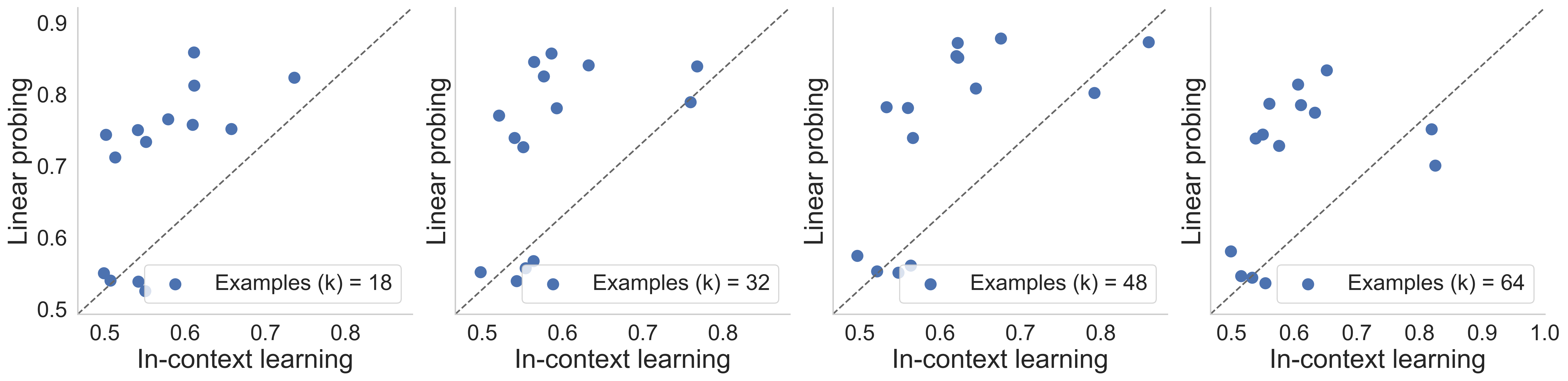
(a) GPT-Neo (125M)

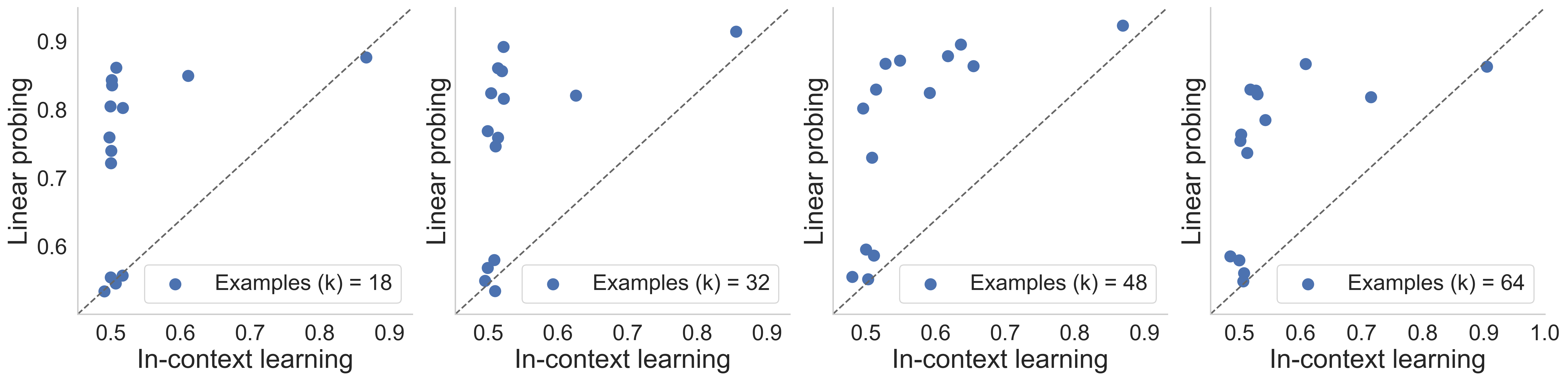
(b) Pythia (160M)

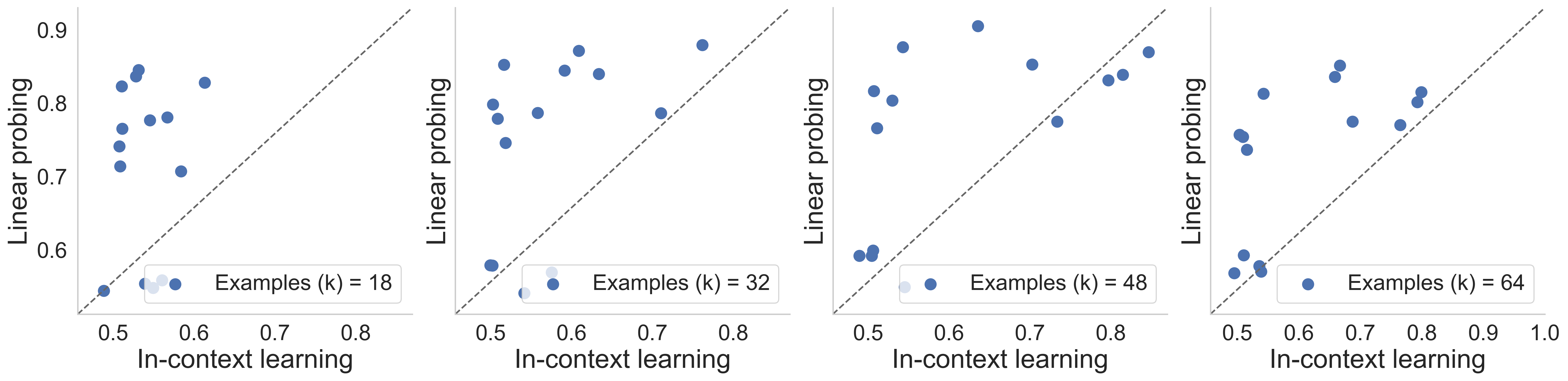
(c) Bloom (560M)

Figure 10: Linear probing vs. in-context learning. Scatter plot of accuracy of in-context learning vs. linear probing on model embeddings across model families and different number of in-context examples: linear probing consistently outperforms in-context learning indicating that the learned representations have sufficient information. Each point in the plot represents a dataset.

In-context learning.

To understand the representation and reasoning gaps for in-context learning, we evaluated three accuracies: a) using in-context learning with base models, b) fine-tuning the model for the task, and c) linear probing the model specifically for the task. The gap due to representation was taken to be the difference between the fine-tuning and linear probing accuracies while the reasoning gap was the gap between linear probing and in-context learning, as described in eq. (1).

In Figure 9, we show the average accuracies of in-context learning, linear probing, and fine-tuning across the 6 tasks. Linear probing closes the gap between in-context learning and fine-tuning, while being task-specific. In Figure 10, we show a scatter plot of the accuracies of linear probing vs. the accuracies of base in-context learning. Linear probing consistently out performs in-context learning showing that the learned representations across these models have sufficient information to complete the tasks but lack reasoning abilities.

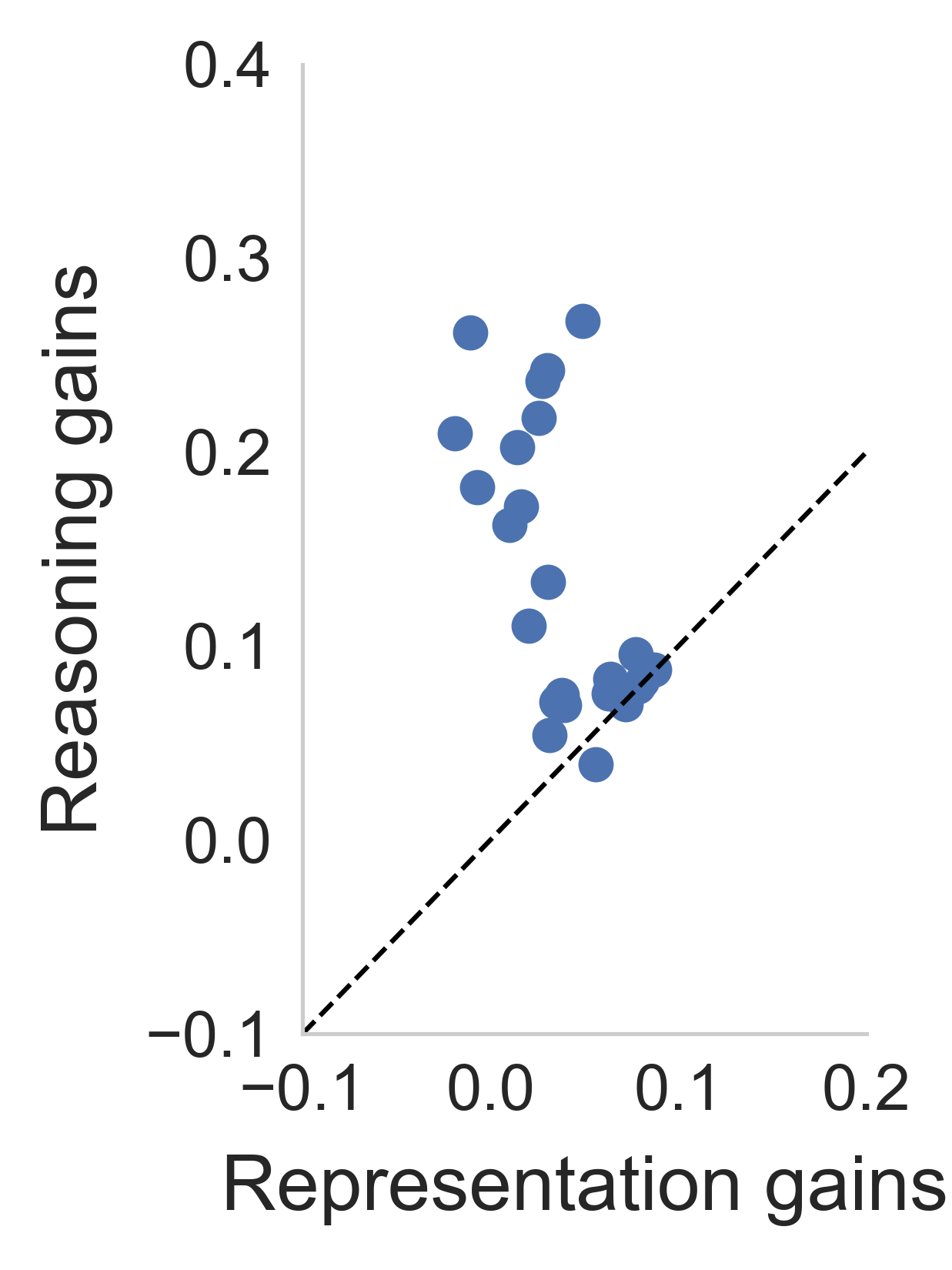
(a) GPT-Neo (125M)

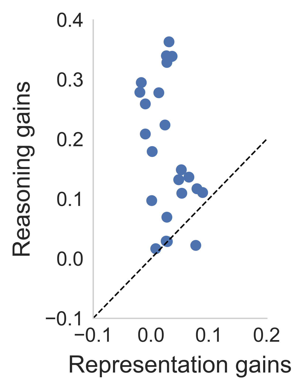
(b) Pythia (160M)

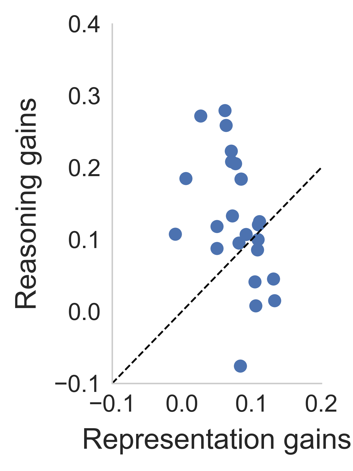
(c) Bloom (560M)

Figure 11: Effects of fine-tuning on reasoning. Across datasets (each point in plot represents a dataset) and model families, fine-tuning improves task-specific reasoning which improves it performance over base in-context learning.

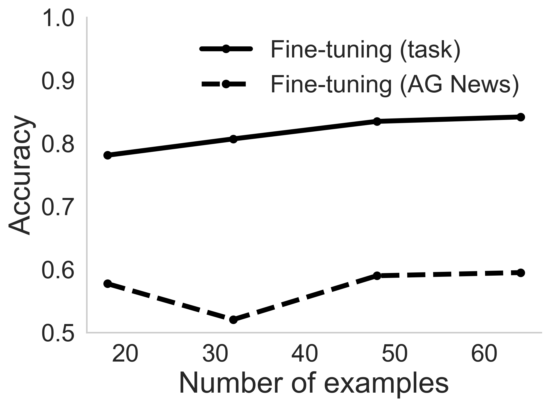
(a) GPT-Neo (125M)

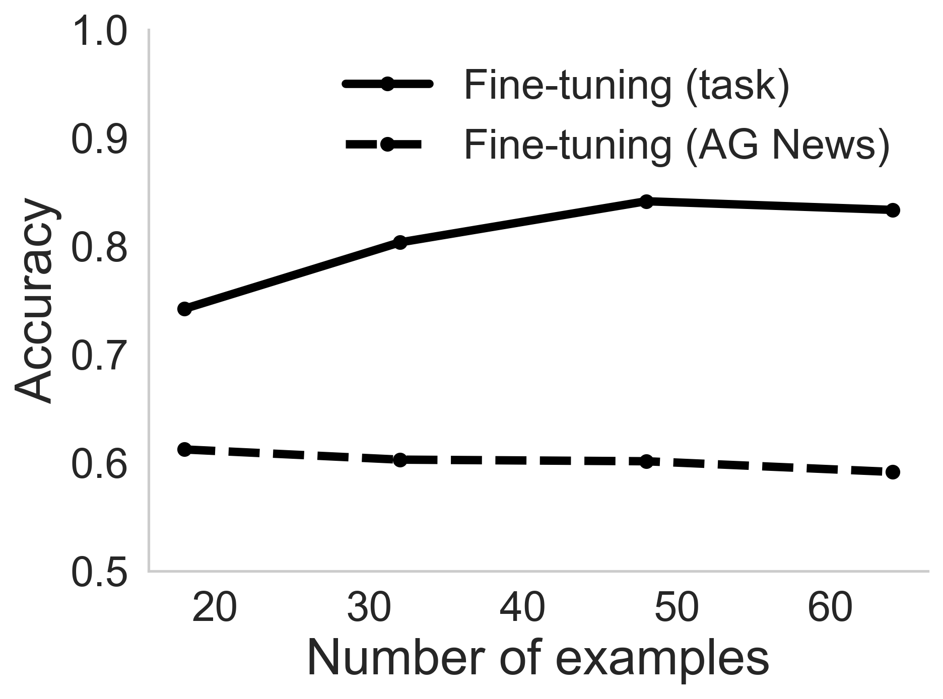
(b) Pythia (160M)

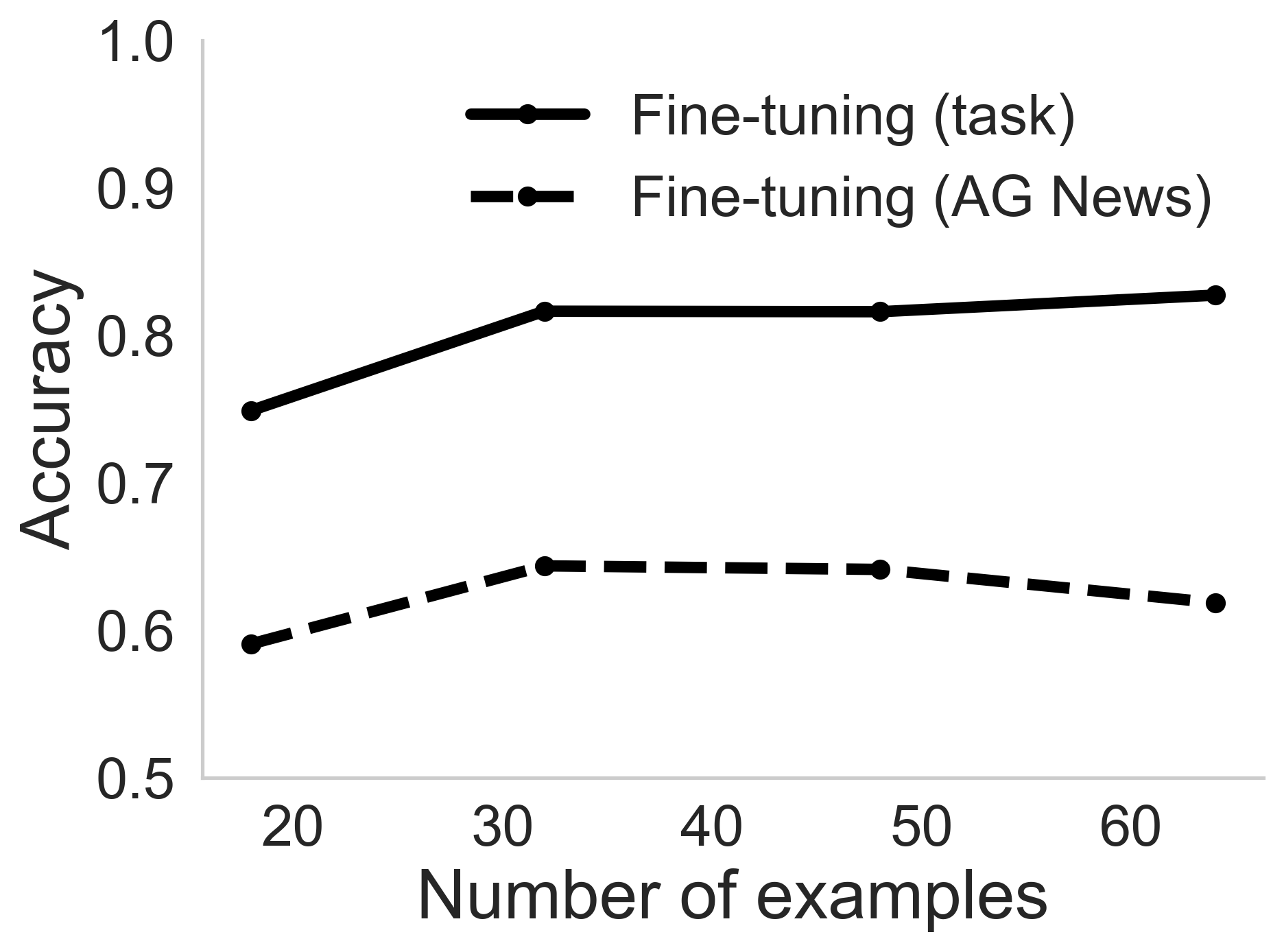
(c) Bloom (560M)

Figure 12: Effects of fine-tuning on task-agnosticity Accuracy of task-specific fine-tuned model vs. accuracy of model fine-tuned on AG-News-0 and evaluated on task. Fine-tuning hurts task-agnosticity across all three model families.

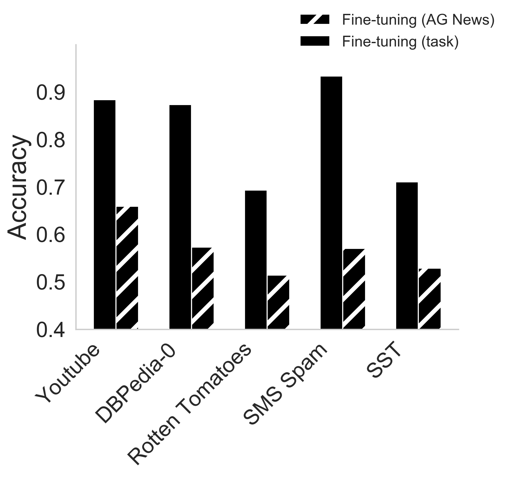
(a) GPT-Neo (125M)

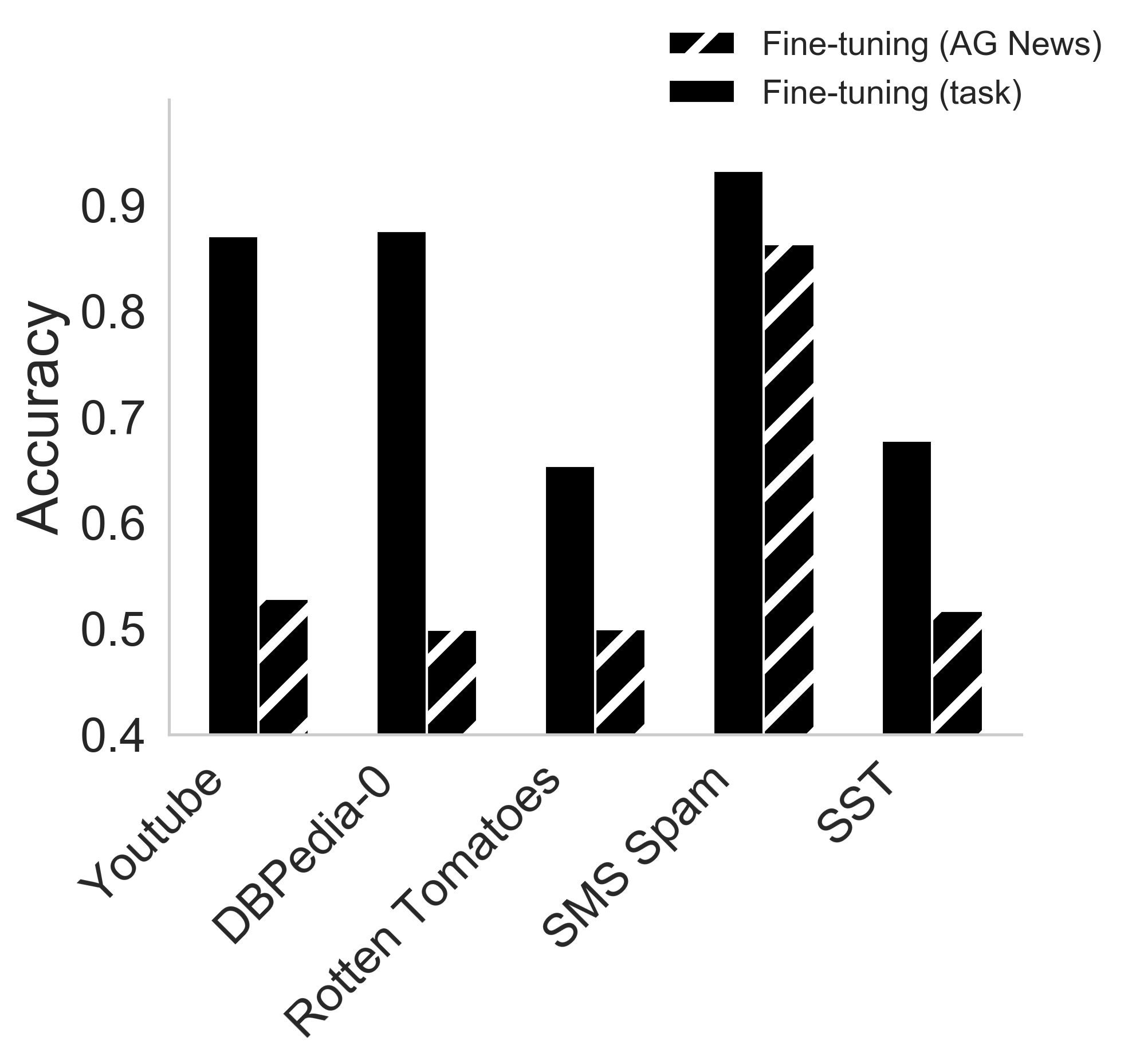
(b) Pythia (160M)

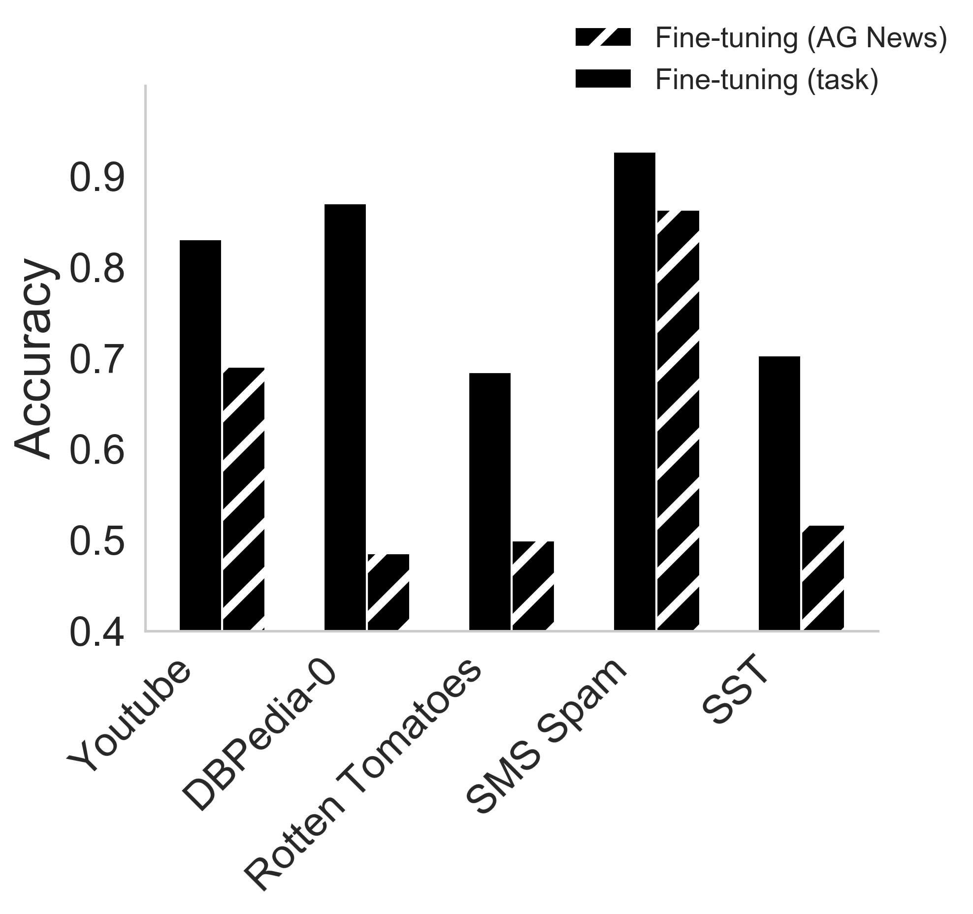
(c) Bloom (560M)

Figure 13: Effects of fine-tuning on task-agnosticity (dataset level) Accuracy of task-specific fine-tuned model vs. accuracy of model fine-tuned on AG-News-0 and evaluated on task. Fine-tuning consistently hurts task-agnosticity across all three model families and datasets.

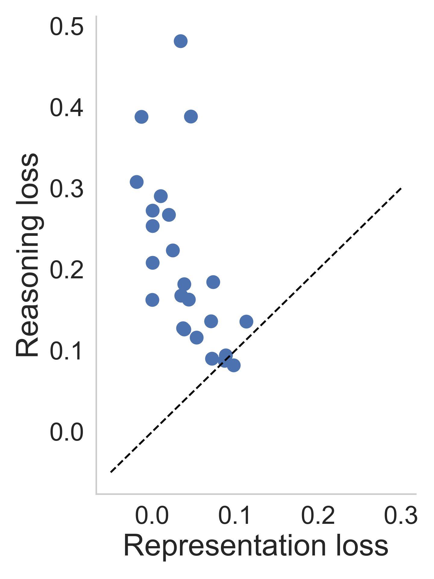
(a) GPT-Neo (125M)

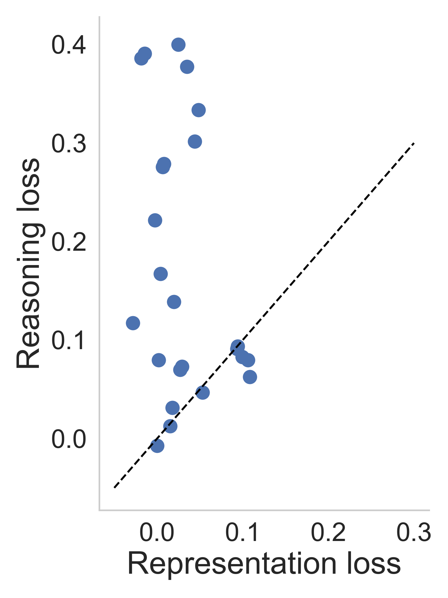
(b) Pythia (160M)

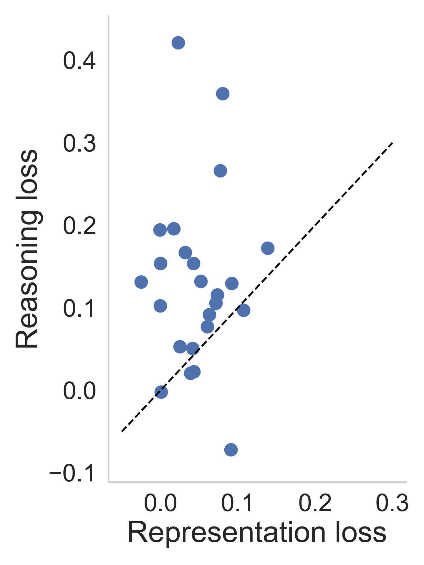
(c) Bloom (560M)

Figure 14: Effects of fine-tuning on task agnosticity. Scatter plot of reasoning loss against representation loss when the base model is trained on AG-News-0 and evaluated on other tasks. Across datasets (each point in plot represents a dataset), fine-tuning majorly impairs reasoning when transferring to tasks outside the specific fine-tuned task.

Fine-tuning.

For the fine-tuning approach, we are interested in understanding two hypotheses: a) how does fine-tuning improve the model performance, and b) whether fine-tuning hurts task-agnosticity of the base model and if yes, what is the underlying reason for it.

For the first hypothesis, we evaluate the proportion of gains that can be attributed to improved representations of the the underlying model. This is computed as the difference in performance of linear probing over the base model and over the fine-tuned model — this evaluates how much the representations have changed specifically for this task. The reasoning gains are then computed by subtracting the representation gains from the total gain (fine-tuning accuracy minus in-context accuracy). Figure 11 shows a scatter plot of these representation gains and reasoning gains, plotted across different datasets and number of examples ($k$). Most of the gains which are realized by fine-tuning are because of improved task-specific reasoning capabilities across the model families.

For the second hypothesis, we first evaluate whether fine-tuning hurts task-agnosticity. For this we evaluate two sets of accuracies: accuracy of a model fine-tuned for the specific task and the accuracy of a model on the task but fine-tuned on the AG News dataset. From Figures 12 and 13, we see that there is a drop in accuracy—over $25.77\%$ across models and datasets. For the second part, we again decompose the drop in accuracy into a representation drop and a reasoning drop. The representation drop is computed by training a linear probe over the two models (task-specific fine-tuned and AG News fine-tuned) and looking at the difference between them. The reasoning drop, as before, is computed by subtracting this representation drop from the total drop. Figure 14 shows that most of this drop in task-agnosticity can be attributed to over-fitting of the reasoning abilities over the task for which the models are fine-tuned.

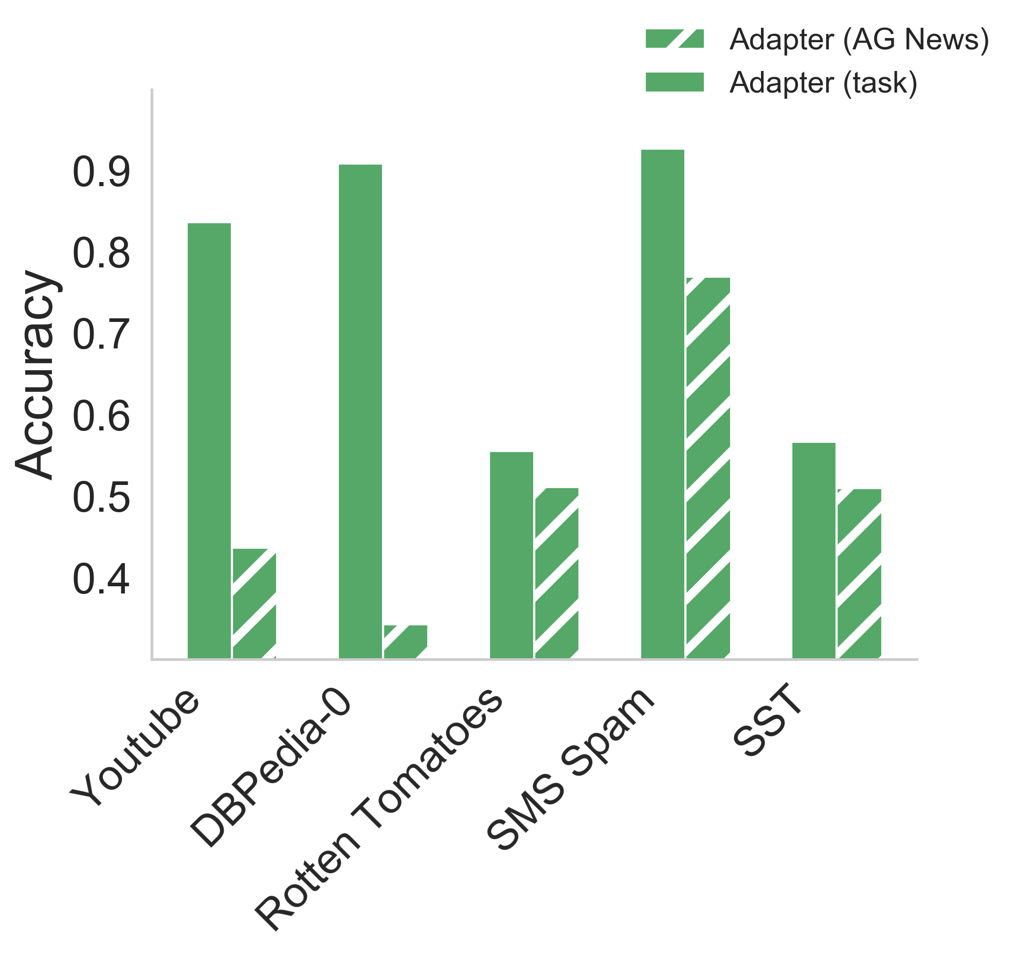
(a) GPT-Neo (125M)

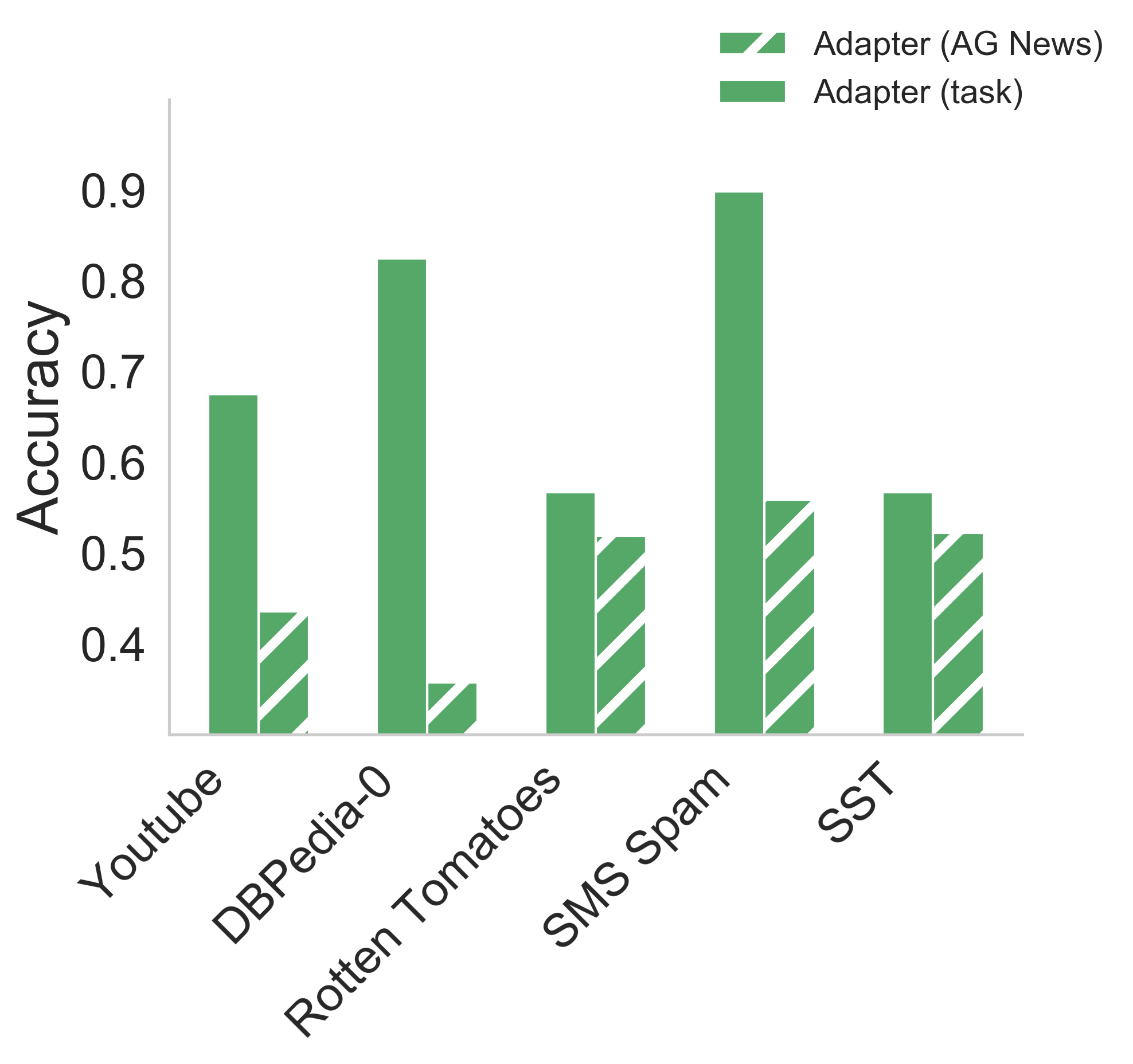
(b) Pythia (160M)

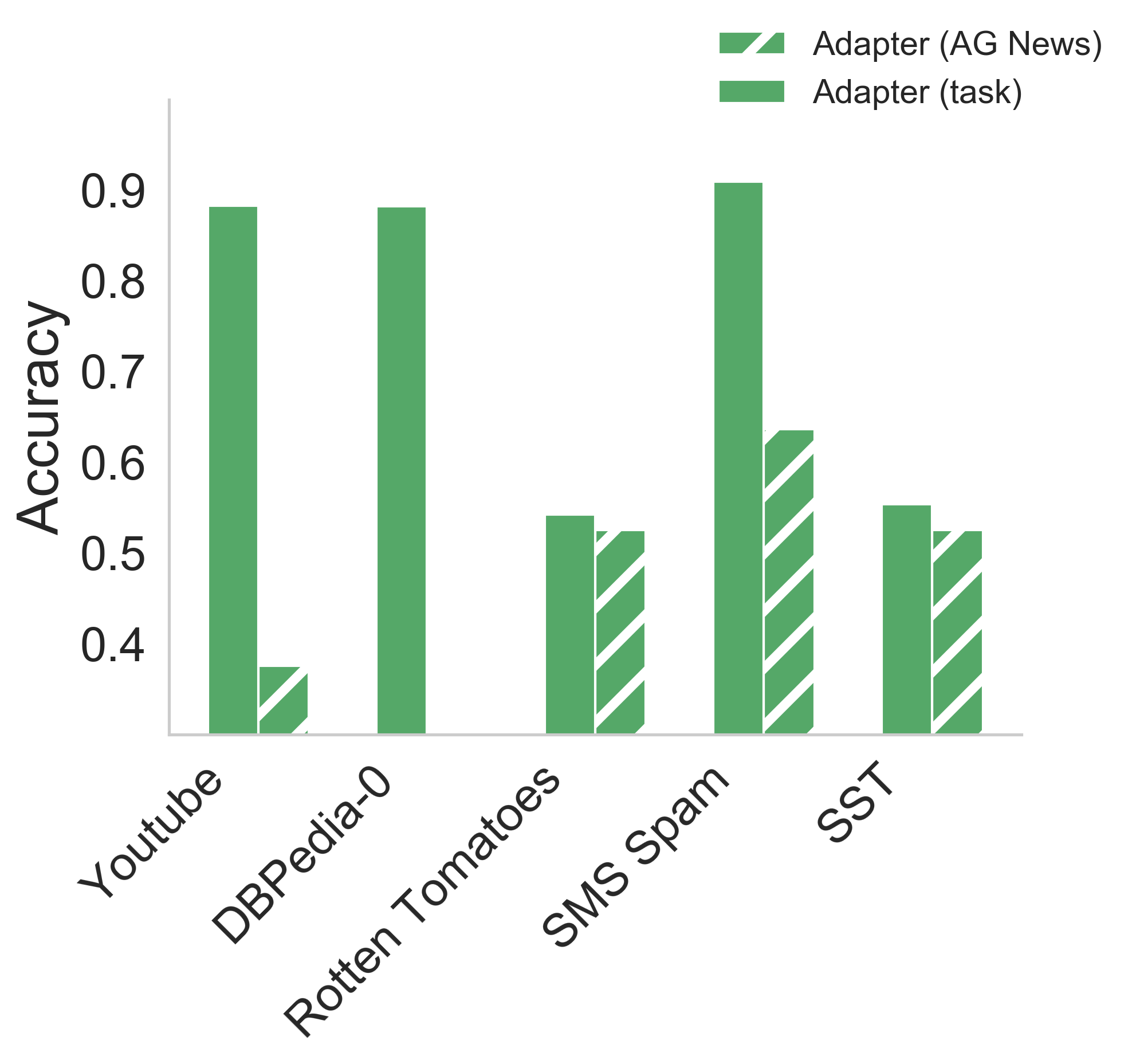
(c) Bloom (560M)

Figure 15: Effects of fine-tuning on task-agnosticity of adapters. Accuracy of task-specific fine-tuned adapter vs. accuracy of adapter fine-tuned on AG-News-0 and evaluated on task. Fine-tuning consistently hurts the generalization ability of adapters across datasets.

Adapters.

Since adapters do not modify the underlying representations of the model, we look at how a single adapter generalizes across tasks. For this we train an adapter on the AG News dataset and evaluate it on the other datasets. We compare this set of accuracies with those obtained by task-specific adapters in Figure 15. The main conclusion is that task-specific adapters are not agnostic learners and over-fit to the task for which they are fine-tuned.

Appendix C Details for Tart implementation

This section contains the details on training Tart’s reasoning module and extended results on the choice of embeddings from Section 4.

C.1 Tart’s reasoning module

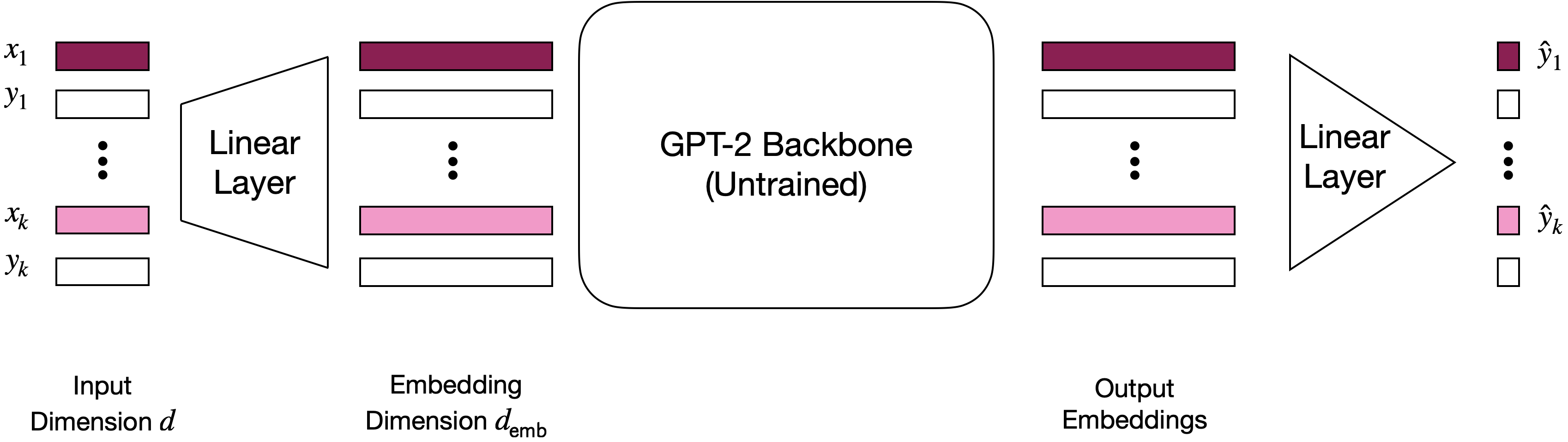
Figure 16: Tart reasoning module architecture. The reasoning module takes as input sequences of $(x,y)$ pairs of dimension $d$. A linear layer is used to project $d$ to the hidden dimension size of the GPT-2 backbone. Finally, a linear layer is applied to the outputs of the backbone to generate predictions for each $x_{k}$ in the input sequence.

Architecture details.

We use the standard GPT-2 architecture [Rad+18] for training our reasoning module. We set the embedding size to 256, number of decoder layers to 12, and number of heads to 8 for a total of 22 million parameters. Since the GPT-2 backbone outputs a sequence of embeddings, we additionally add a linear layer in the end to convert the output to scalar values (see Figure 16). Additionally, the binary labels $y$ are encoded as a one-hot vector to match the input dimension $d$ of the corresponding covariates $x$.

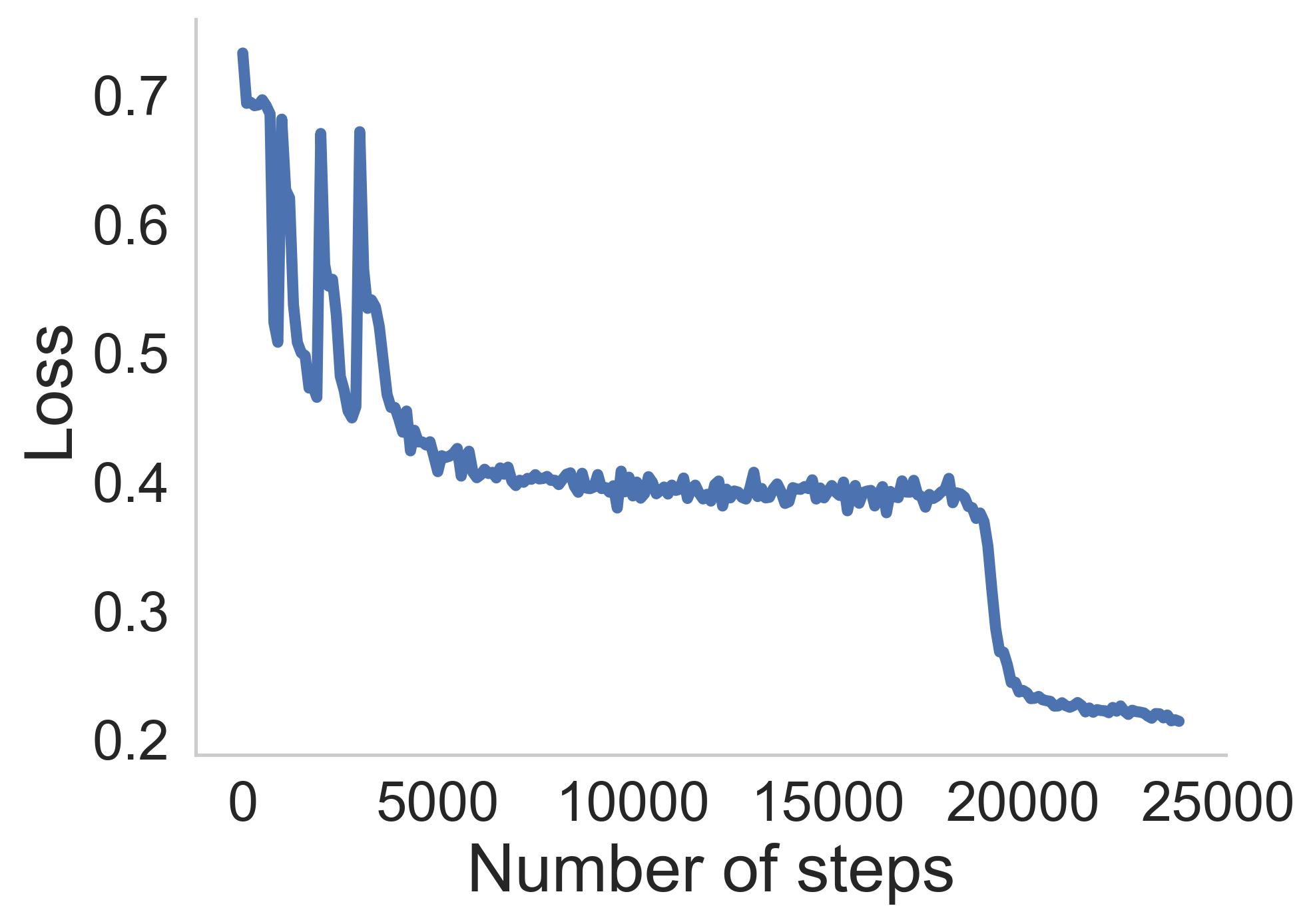
Figure 17: Training loss vs. number of steps. The plot shows the variation in training loss as a function of the number of steps of gradient descent for Tart’s reasoning module.

Training procedure.

We trained Tart’s reasoning module with a context length of 258 (allowing for up to 256 in-context examples). The batch size was set to 64, learning rate to 0.0001 and the model was trained for a total of 24000 epochs. Each batch of training data consists of sampling a sequence of 258 examples using eq. (3). In addition to these hyperparameters, we used a curriculum on the input dimensions and on the number of examples in the sequence to train our module—the input dimensions started from a value of 4 and were incremented by 4 every 1000 epochs while the number of examples started from 18 and were incremented by 30 every 1000 epochs.

Combining reasoning module with base LLM.

We trained the reasoning module with input dimension set to 16. However, most base models produce representations which are much higher dimensional (ranging from 784 to 2048). In order to reduce the dimensionality of these representations, we perform PCA on the output embeddings of the base model, learning the components using only the training points available for that specific task. The test examples are then projected onto these principal components to produce 16 dimensional input representations.

(a) GPT-Neo (125M)

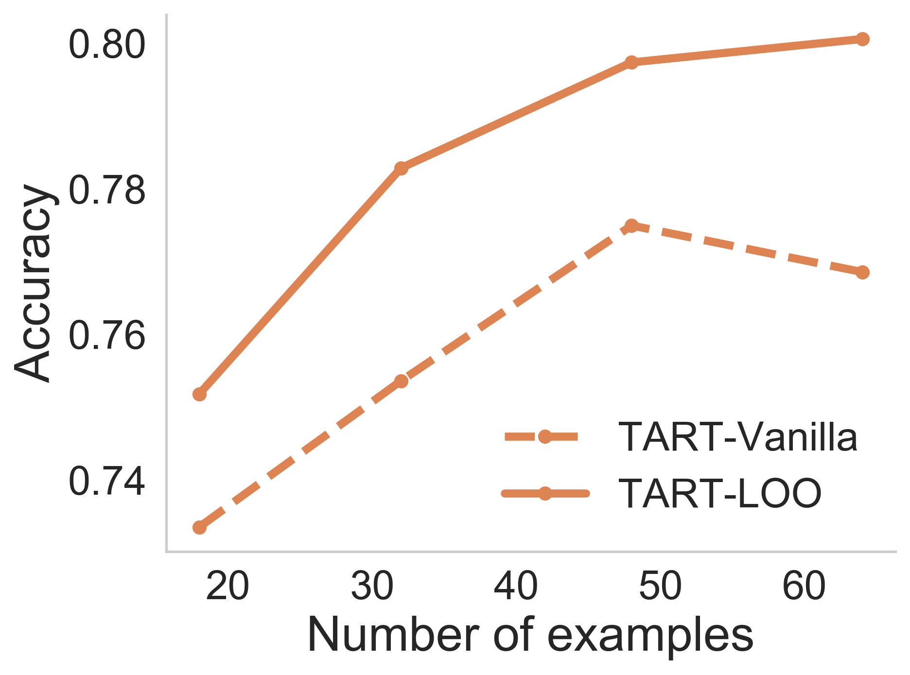
(b) Pythia (160M)

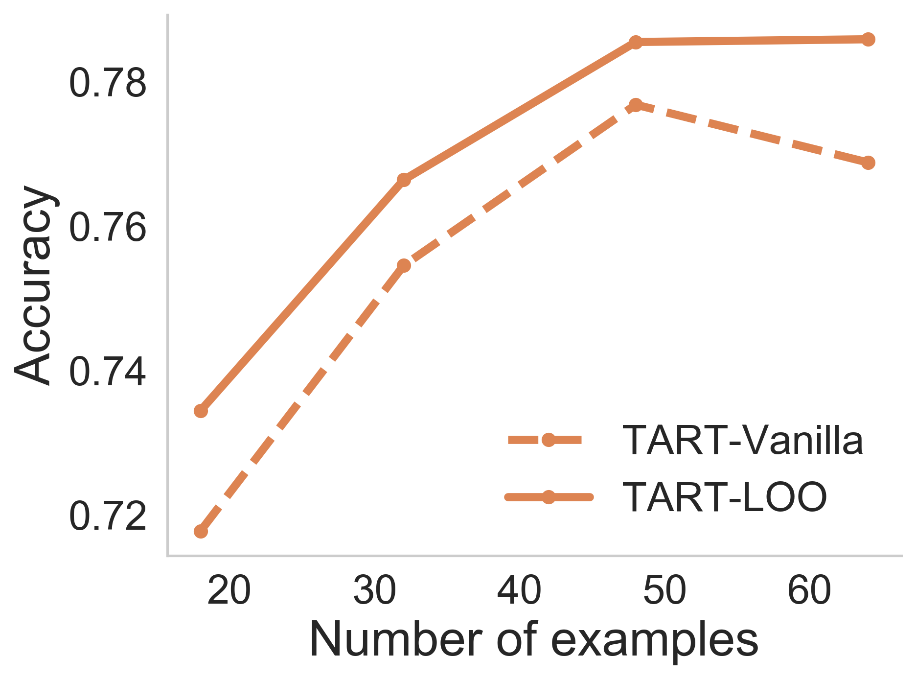
(c) Bloom (560M)

Figure 18: LOO embeddings vs. Vanilla Embeddings. Comparison of Tart performance when using LOO embeddings and vanilla embeddings. Vanilla embeddings see a performance collapse, but LOO embeddings do not.

(a) Vanilla embeddings

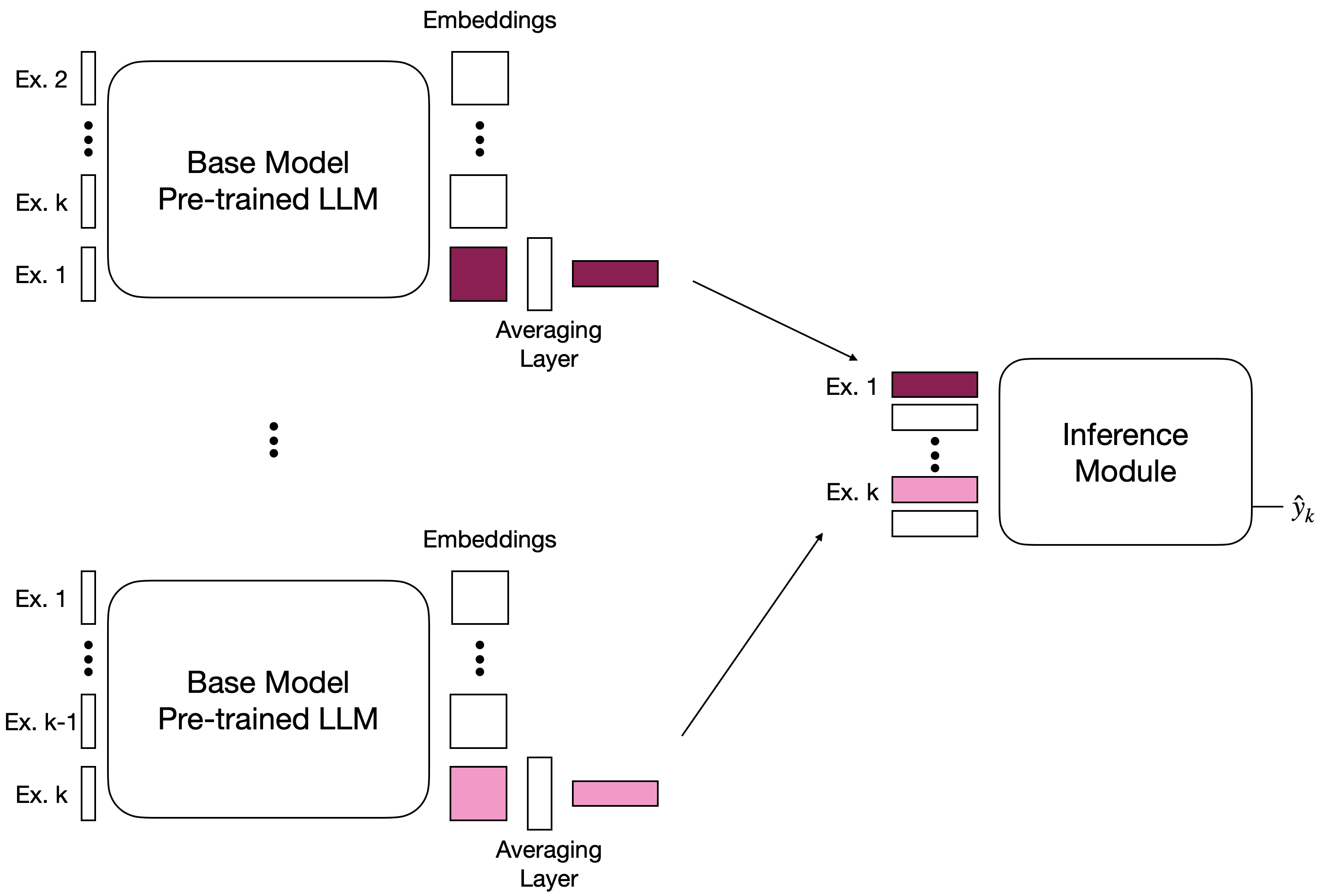
(b) LOO embeddings

Figure 19: Tart Embedding Protocols. (a) For the vanilla embeddings, the test example is appended to the training set and the sequence is passed to the base model. The representation for each train example in this sequence is taken as the average embedding across all its tokens. (b) For the LOO embeddings, we generate embeddings for each train example separately by placing all the other train examples before it in the prompt and averaging the embeddings over the final example’s tokens.

C.2 Choice of representations

As discussed in Section 4.2 there are two possible options for forming the representations, the vanilla embeddings and the leave-one-out (LOO) embeddings. Figure 19 shows the schematic differences between the two style of embedding. In Figure 18, we plot the average accuracies across different datasets for both vanilla and LOO embeddings, observing that the LOO embeddings consistently perform better across the different model families.

C.3 Proof of Theorem 1

In this section, we provide a formal statement of Theorem 1 from Section 4.3. Our theorem quantifies the expected error of the Transformer, trained on synthetic data, on natural language tasks in terms of the change in the two input distributions.

We begin by introducing some notation. We denote the class of Transformer family by

$$\mathcal{T}_{\Theta}:\,=\{T_{\theta}:^{(2k+1)\times d}\mapsto\quad|\quad\theta\in\Theta\}\;,$$ (7)

where $k$ represents the maximum number of in-context examples the Transformer can support, $d$ represents the input dimensions, and $\Theta$ represents the corresponding parameter class over which the Transformer family is defined.

Observe that the Transformer family $\mathcal{T}_{\Theta}$ takes as input a sequence of $k$ train examples, each corresponding to two tokens of hidden dimension $d$: a covariate $x\in^{d}$ and a binary label, encoded as a one-hot vector in $d$ dimension. This sequence of train examples is followed by a test example, for which we only have the features $x_{k+1}$.

Given this background, let $P_{{\sf syn}}$ denote the synthetic distribution over sequences $\{(x_{1},y_{1}),\ldots,(x_{k},y_{x}),(x_{k+1})\}$. Similarly, let $P_{{\sf NL}}$ denote the corresponding distribution over sequences derived from natural language tasks where $x_{i}$ denotes the LLM embeddings of the example. Recall from Section 4.1.1, the synthetic training distribution $P_{{\sf syn}}$ is given by

$$\text{Sequence }s_{t}:w_{t}\sim\mathcal{N}(0,I_{d}),\quad x_{i,t}\sim\mathcal{N}(0,I_{d}),\quad y_{i,t}\sim\sigma(\alpha\langle x_{i,t},w_{t}\rangle)\qquad\text{for }i\in[k]\;,$$ (8)

for each training point $(x_{i,t},y_{i,t})$. The test point is also sampled similarly from an independent standard normal distribution. Let $\ell:\times\mapsto$ be the loss function used for evaluating the performance of the reasoning module. Further, let use denote the expected loss under a distribution $P$

$${\sf err}_{P}(T):\,=\mathbb{E}_{(s,y)\sim P}[\ell(T(s),y)]\;,$$ (9)

and the corresponding empirical distribution over samples $S$ by $\hat{{\sf err}}_{P}$, where the dependence on the samples is implicit. Given these samples, we denote the empirical risk minimizer

$$T_{S}=\arg\min_{T\in\mathcal{T}_{\Theta}}\frac{1}{|S|}\sum_{s\in S}\ell(T(s),y)\;.$$ (10)

In addition to these notation, we make the following Lipschitz assumption on the the loss function $\ell$ and the Transformer model $T$.

Assumption 1.

[Lipschitz loss.] For any two output labels $y,y^{\prime}$, the loss function $\ell$ is Lipschitz with constant $c_{1}$, that is,

$$|\ell(Tr(s),y)-\ell(Tr(s),y^{\prime})|\leq c_{1}|y-y^{\prime}|\;.$$ (11)

Assumption 2.

[Lipschitz models.] For any two input sequences $s,s^{\prime}$, each any model $T\in\mathcal{T}_{\Theta}$ is Lipschitz with constant $L$, that is,

$$|T(s)-T(s^{\prime})|\leq L\|s-s^{\prime}\|.$$ (12)

Given this setup, we are now ready to state a formal version of Theorem 1.

Theorem 2 (Formal version of Theorem 1).

Let $T_{S}\in\mathcal{T}_{\Theta}$ denote the trained reasoning module on set $S$ of synthetic logistic regression tasks with $n_{{\sf syn}}$ sequences sampled from distribution $P_{{\sf syn}}$ in eq. (3). Let the loss function $\ell$ satisfy Assumption 1 and the model class $\mathcal{T}_{\Theta}$ satisfy Assumption 2. Then, with probability at least $1-\delta$, we have

$${\sf err}_{P_{{\sf NL}}}(T_{S})\leq c_{1}\max(1,L)\cdot W_{1}(P_{{\sf NL}},P_{{\sf syn}})+c_{1}\cdot\sqrt{\frac{2\text{VC}(\mathcal{T}_{\Theta})\ln m}{n_{{\sf syn}}}}+4\sqrt{\frac{2\ln(4/\delta)}{n_{{\sf syn}}}}+\hat{{\sf err}}_{P_{{\sf syn}}}(T_{S})\;,$$ (13)

where $W_{1}$ denotes the Wasserstein-1 metric and $\text{VC}(\mathcal{T}_{\Theta})$ represents the VC dimension of class $\mathcal{T}_{\Theta}$

Proof.

We begin by decomposing the error ${\sf err}_{P_{{\sf NL}}}(T_{S})$ into three components as

$${\sf err}_{P_{{\sf NL}}}(T_{S})=\underbrace{{\sf err}_{P_{{\sf NL}}}(T_{S})-{\sf err}_{P_{{\sf syn}}}(T_{S})}_{\text{(I)}}+\underbrace{{\sf err}_{P_{{\sf syn}}}(T_{S})-\hat{{\sf err}}_{P_{{\sf syn}}}(T_{S})}_{\text{(II)}}+\hat{{\sf err}}_{P_{{\sf syn}}}(T_{S})\;.$$ (14)

We now upper bound each of the terms (I) and (II) separately.

Bound on Term (I).

Let $\gamma$ denote an arbitrary joint distribution over the distributions $P_{{\sf syn}}$ and $P_{{\sf NL}}$. Then, we can bound the first term as

$${\sf err}_{P_{{\sf NL}}}(T_{S})-{\sf err}_{P_{{\sf syn}}}(T_{S}) =\mathbb{E}_{P_{{\sf NL}}}[\ell(T(s),y)]-\mathbb{E}_{P_{{\sf syn}}}[\ell(T(s^{\prime}),y^{\prime})]$$

$$\stackrel{{\scriptstyle{\sf(i)}}}{{=}}\mathbb{E}_{\gamma}[\ell(T(s),y)-\ell(T(s^{\prime}),y^{\prime})]$$

$$\stackrel{{\scriptstyle{\sf(ii)}}}{{\leq}}\inf_{\gamma}\mathbb{E}_{\gamma}\left|\ell(T(s),y)-\ell(T(s^{\prime}),y^{\prime})\right|\;,$$ (15)

where ${\sf(i)}$ follows from the independence of the two expectations and ${\sf(ii)}$ follows from that ${\sf(i)}$ holds for any arbitrary joint distribution $\gamma$. The final bound on this term now follows:

$$\inf_{\gamma}\mathbb{E}_{\gamma}\left|\ell(T(s),y)-\ell(T(s^{\prime}),y^{\prime})\right| =\inf_{\gamma}\int\left|\ell(T(s),y)-\ell(T(s),y^{\prime})+\ell(T(s),y^{\prime})-\ell(T(s^{\prime}),y^{\prime})\right|d\gamma$$

$$\stackrel{{\scriptstyle{\sf(i)}}}{{\leq}}c_{1}\inf_{\gamma}\int|y-y^{\prime}|-\|T(s^{\prime})-T(s)\|d\gamma$$

$$\stackrel{{\scriptstyle{\sf(ii)}}}{{\leq}}c_{1}\max(1,L)\cdot\inf_{\gamma}\int|y-y^{\prime}|-\|s^{\prime}-s\|d\gamma$$

$$=c_{1}\max(1,L)\cdot W_{1}(P_{{\sf NL}},P_{{\sf syn}})\;,$$ (16)

where the inequalities ${\sf(i)}$ follows from Assumption 1 and ${\sf(ii)}$ follows from Assumption 2. This completes the bound on Term (I).

Bound on Term (II).

Using a standard generalization bound [SB14, see Theorem 26.5], we have with probability at least $1-\delta$

$${\sf err}_{P_{{\sf syn}}}(T_{S})-\hat{{\sf err}}_{P_{{\sf syn}}}(T_{S}) \leq\mathcal{R}(\ell\circ\mathcal{T}_{\Theta})+4\sqrt{\frac{2\ln(4/\delta)}{n_{{\sf syn}}}}$$

$$\leq c_{1}\cdot\mathcal{R}(\mathcal{T}_{\Theta})+4\sqrt{\frac{2\ln(4/\delta)}{n_{{\sf syn}}}}$$

$$\stackrel{{\scriptstyle{\sf(i)}}}{{\leq}}c_{1}\cdot\sqrt{\frac{2\text{VC}(\mathcal{T}_{\Theta})\ln m}{n_{{\sf syn}}}}+4\sqrt{\frac{2\ln(4/\delta)}{n_{{\sf syn}}}}$$ (17)

where $\mathcal{R}(\ell\circ\mathcal{T}_{\Theta})$ denotes the Rademacher complexity of the class $\mathcal{T}_{\Theta}$ composed with the loss function $\ell$ and inequality ${\sf(i)}$ follows from Sauer’s Lemma.

Combining the bounds in equations (C.3) and (C.3) completes the proof of the theorem. ∎

Appendix D Details for experimental evaluation

We describe supplementary experimental details from Section 5 as well as additional results for the natural language benchmark evaluations (Section D.2) and results for other modalities (vision and audio) (Section D.3).

D.1 Experimental setup

We begin by providing dataset statistics and details of the baselines.

Dataset	Test size	Max char	Max token	Avg. char	Avg. token
		length	length	length	length
AG-News-0	3800	732	259	237.07	51.36
AG-News-1	3800	814	213	232.01	51.46
AG-News-2	3800	814	225	236.10	52.25
AG-News-3	3800	892	259	234.86	51.38
Civil Comments	11576	1000	634	272.72	61.73
DBPedia-0	10000	2081	629	300.94	65.83
DBPedia-1	10000	2081	629	298.81	66.91
DBPedia-2	10000	2081	883	286.85	66.53
DBPedia-3	10000	2081	629	275.81	63.88
IMDB	25000	12988	2972	1293.79	292.82
Rotten Tomatoes	1066	261	63	115.52	25.36
SMS Spam	4181	612	258	81.46	23.76
SST	2210	256	60	102.40	22.34
Youtube	250	1125	292	112.50	31.84

Table 2: Dataset (test) statistics for all NLP datasets.

Dataset	Max char	Max token	Avg. char	Avg. token
	length	length	length	length
AG-News-0	701	256	236.15	51.53
AG-News-1	749	180	232.48	51.61
AG-News-2	735	256	241.70	53.91
AG-News-3	1002	258	241.21	53.21
Civil Comments	1000	347	280.97	63.44
DBPedia-0	707	207	300.48	65.79
DBPedia-1	1023	280	299.89	66.57
DBPedia-2	628	203	288.21	66.22
DBPedia-3	758	203	279.45	64.24
IMDB	7068	1630	1284.20	290.00
Rotten Tomatoes	260	62	112.46	24.82
SMS Spam	911	217	106.90	31.87
SST	248	56	101.97	22.34
Youtube	1089	767	90.12	29.98

Table 3: Dataset (train) statistics for all NLP datasets.

D.1.1 Dataset construction and statistics

Table 3 and 2 provides a detailed breakdown of dataset statistics. For each dataset, we use the original test sets with the exception of Civil Comments [Bor+19], AG News [ZZL15] and DBPedia [ZZL15]. For the multi-class datasets—AG News [ZZL15] and DBPedia [ZZL15] — we construct 4 binary classification tasks for each datasets. More concretely, AG News labels news articles into four categories: World, Sports, Business, and Science/Technology. We create a separate binary classification task for each category, sampling negatives from the remaining classes. DBPedia is a 14-way ontology classification dataset. We create 4 separate binary classification tasks for the educational institution, company, artist, and athlete ontologies, sampling negatives from the remaining classes. For the train set, we sample a class-balanced set of 64 examples from the original dataset. For each dataset, we sample 5 separate training sets, using 5 different random seeds. In evaluations, we evaluate Tart and the baseline methods across each of these 5 different training sets.

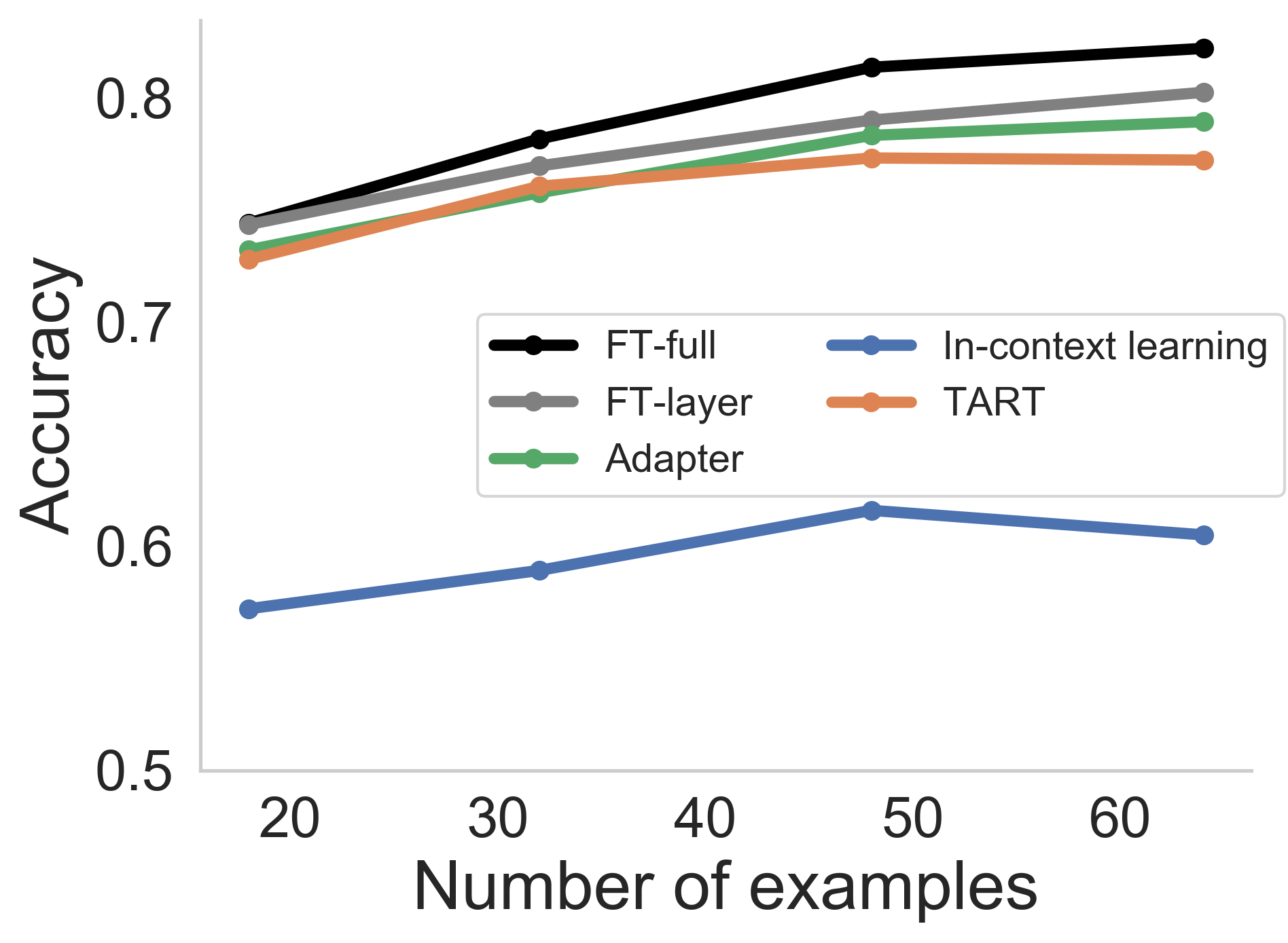
(a) GPT-Neo (125M)

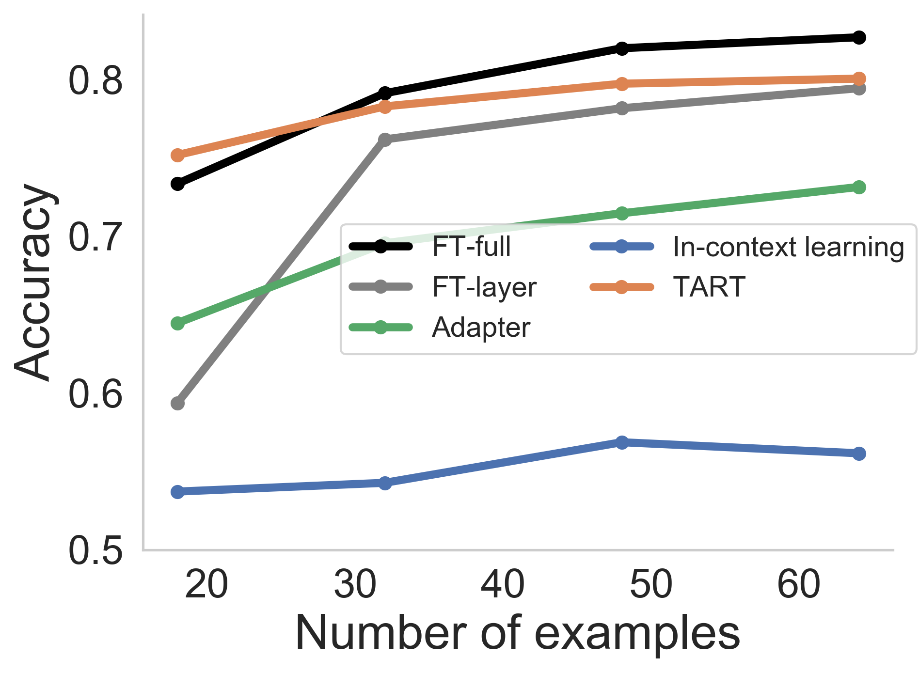
(b) Pythia (160M)

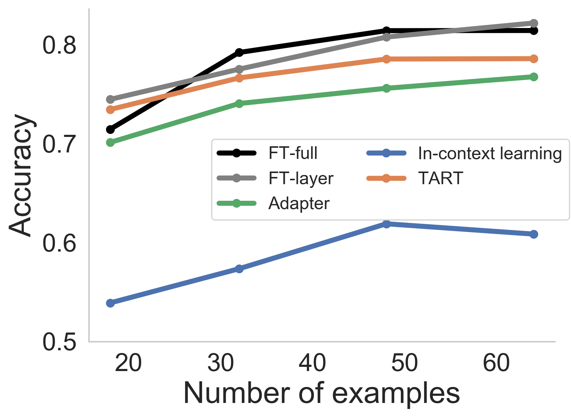
(c) Bloom (560M)

Figure 20: Comparison of all methods. Tart significantly improves base in-context learning performance and is competitive with full-finetuning across model families.

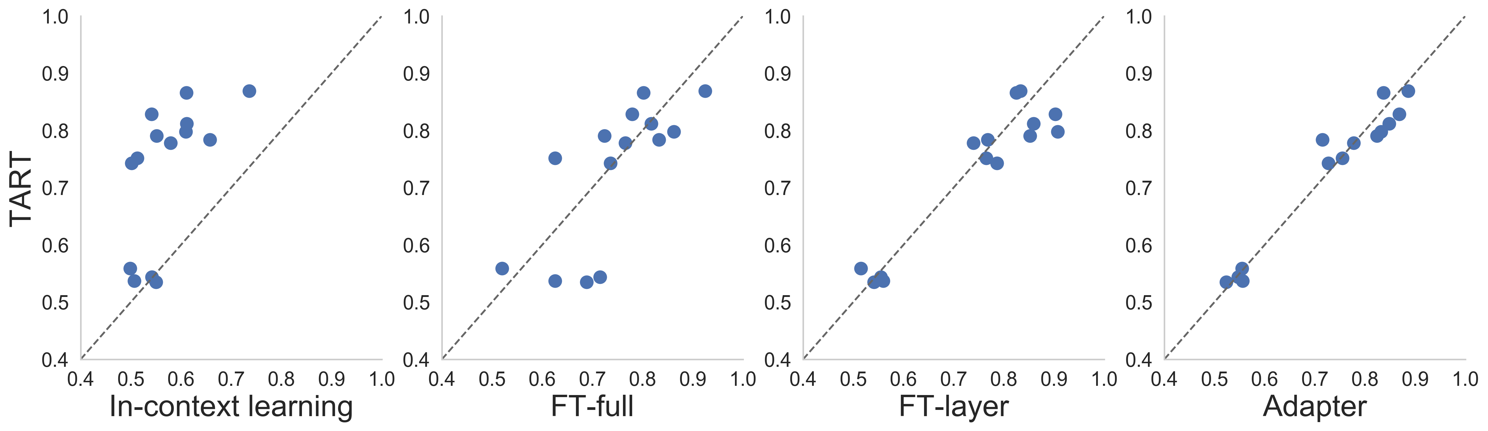
(a) Number of examples = 18

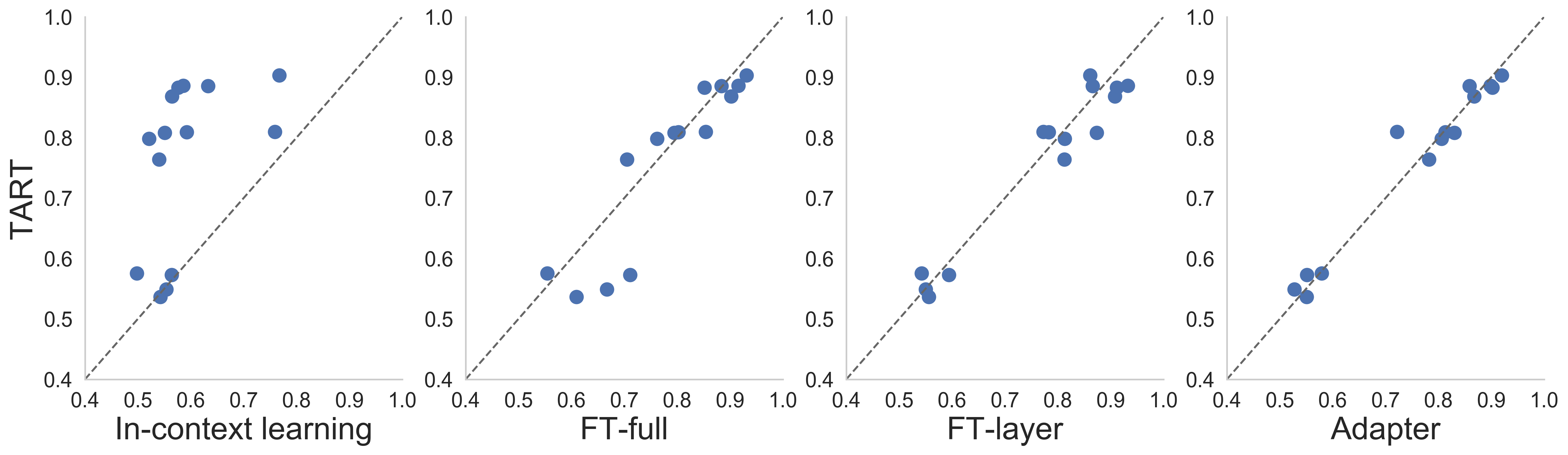
(b) Number of examples = 32

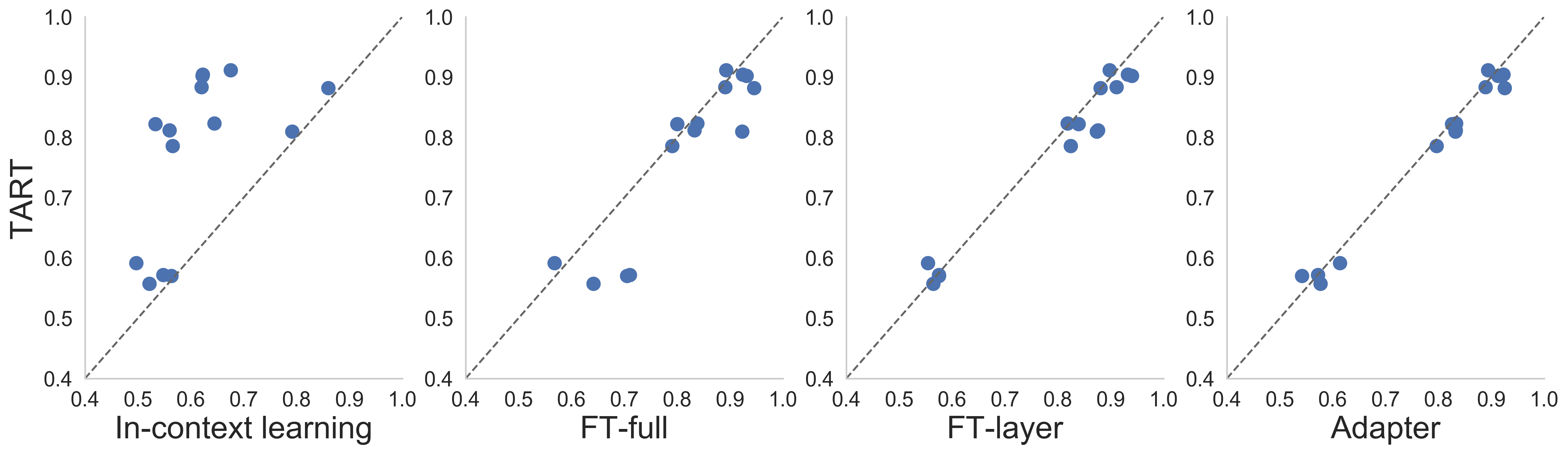
(c) Number of examples = 48

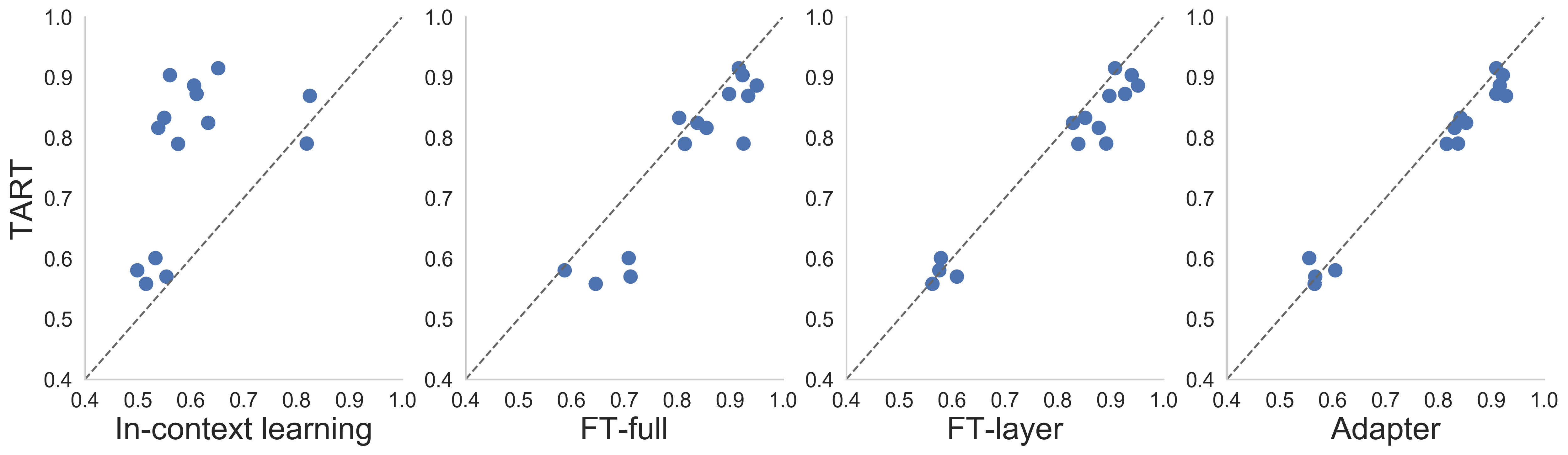
(d) Number of examples = 64

Figure 21: Comparison of Tart and task-adaptation approaches (GPT-Neo (125M)). We see that for GPT-Neo (125M), Tart outperforms in-context learning and is competitive with full fine-tuning and adapters across all $k$.

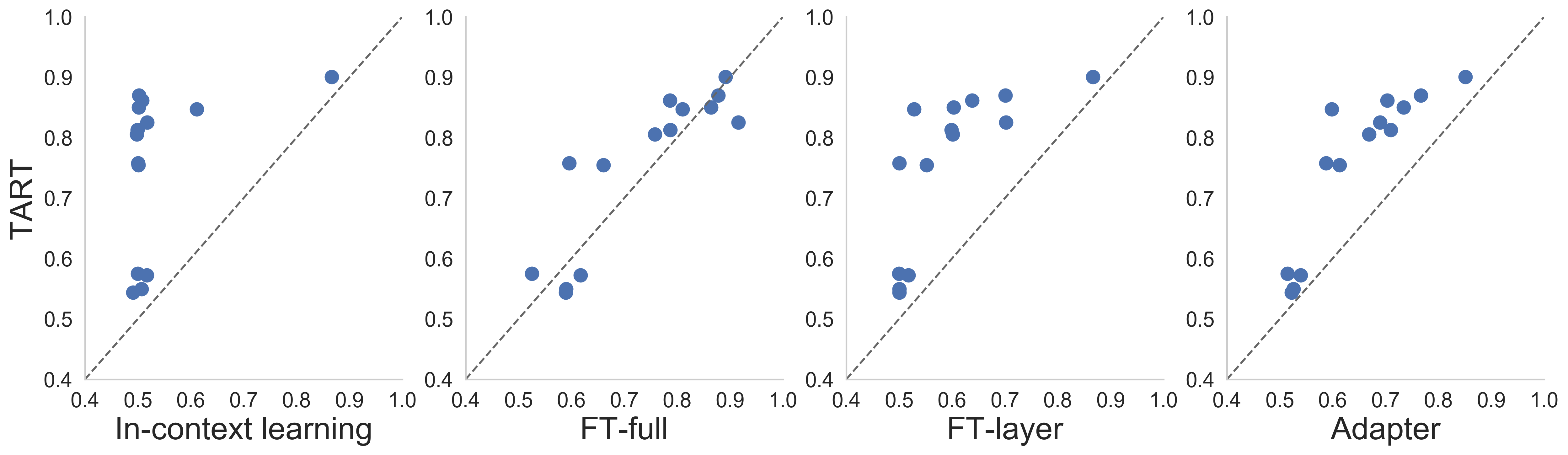
(a) Number of examples = 18

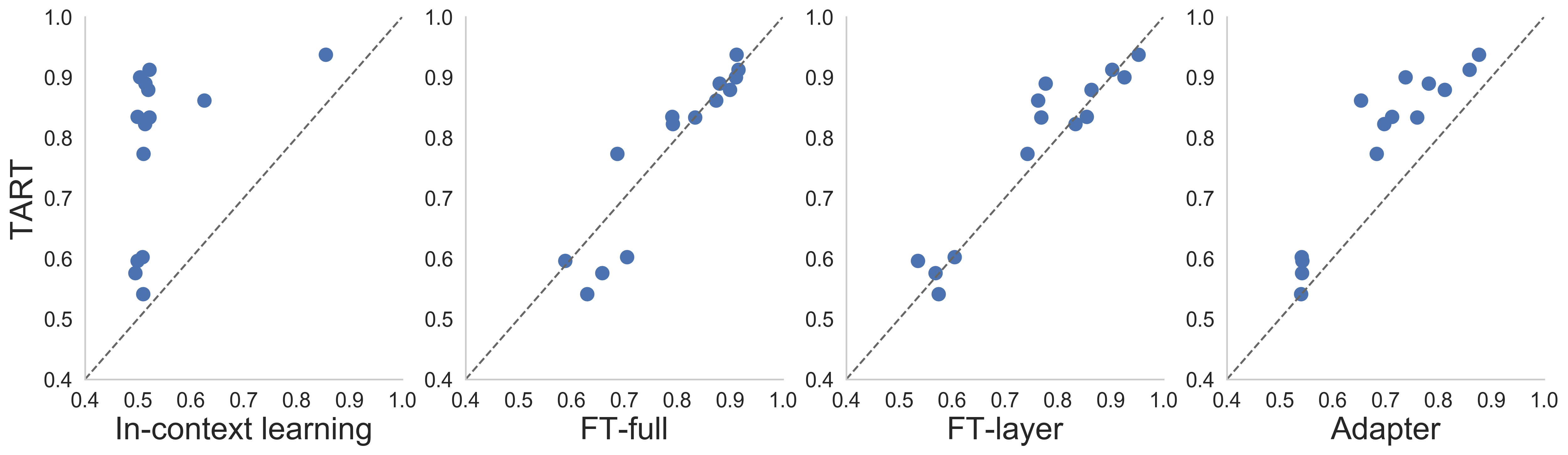
(b) Number of examples = 32

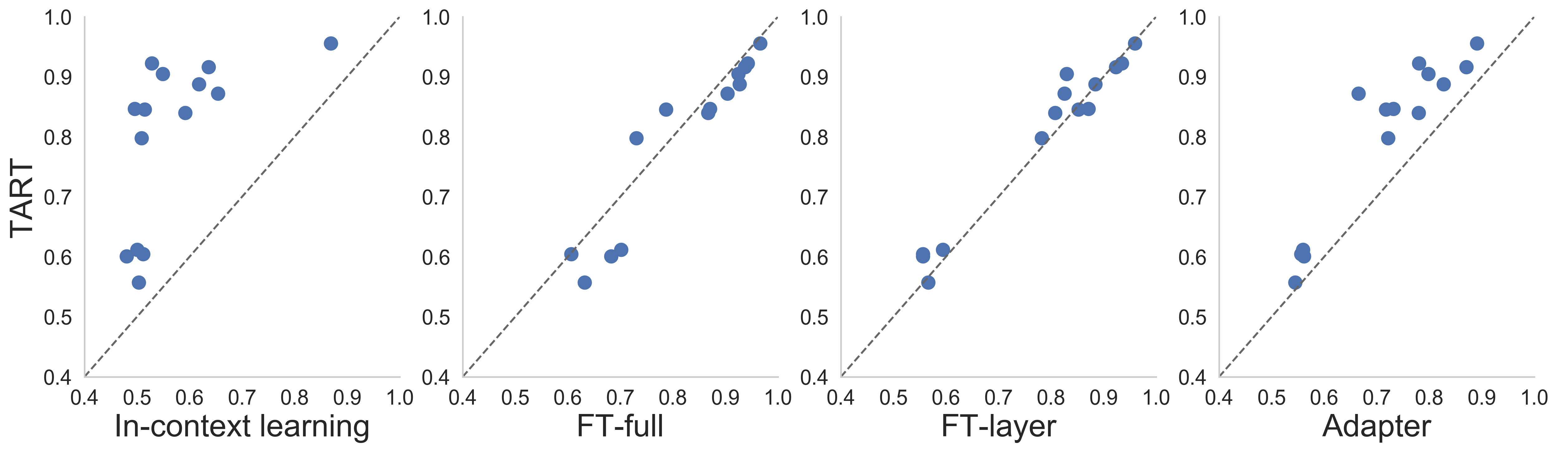
(c) Number of examples = 48

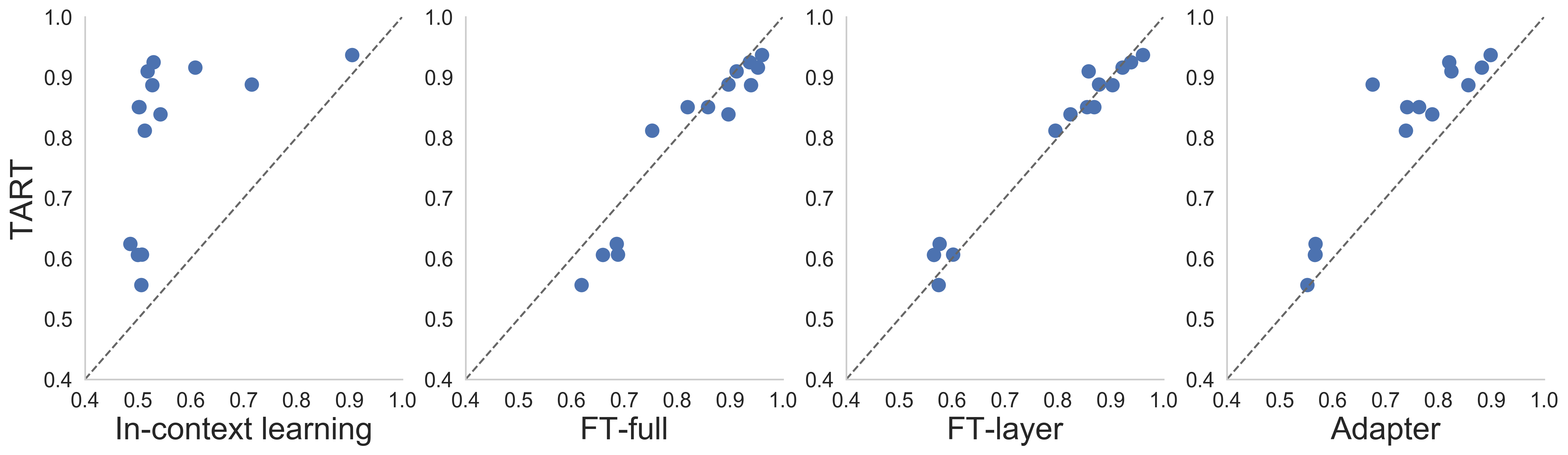
(d) Number of examples = 64

Figure 22: Comparison of Tart and task-adaptation approaches (Pythia (160M)). We see that for Pythia (160M), Tart outperforms in-context learning and adapters and is competitive with full fine-tuning across all $k$.

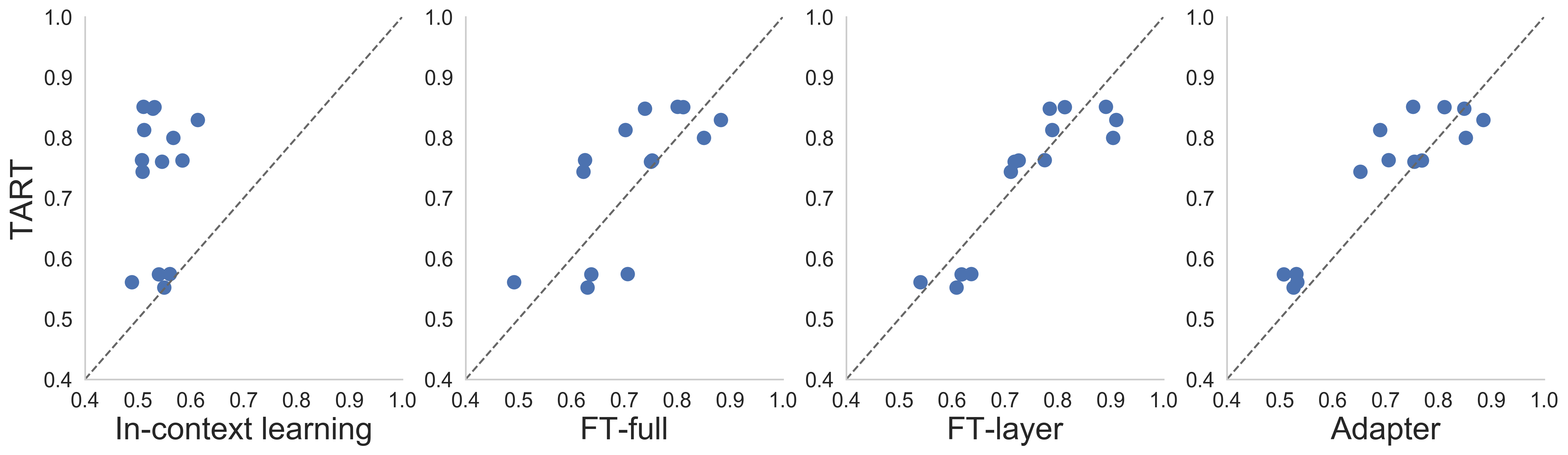
(a) Number of examples = 18

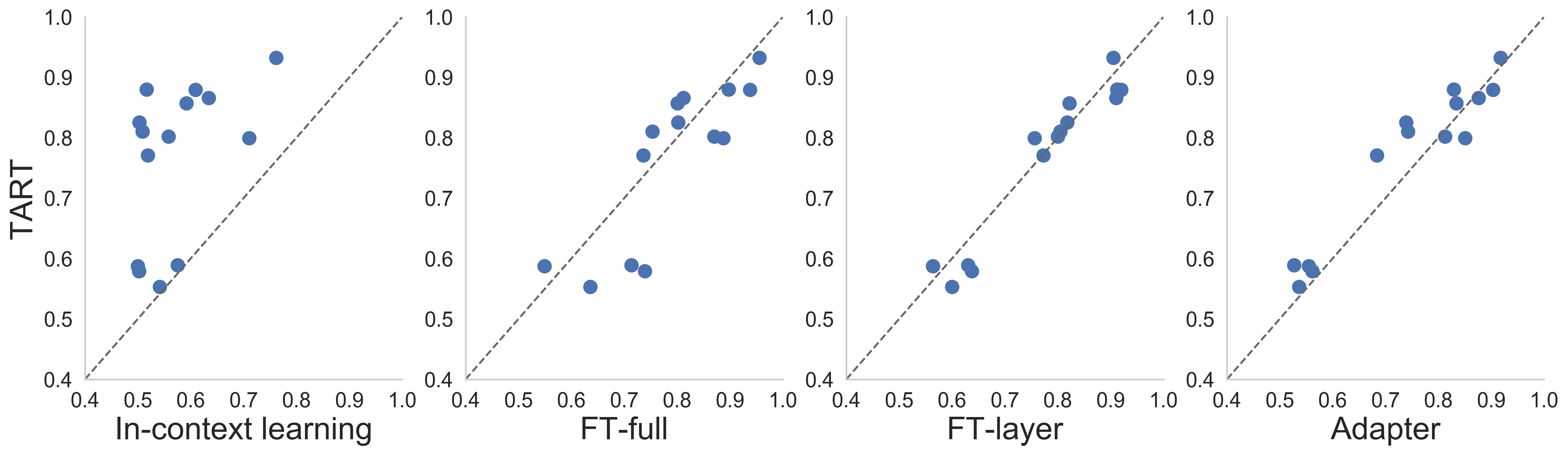
(b) Number of examples = 32

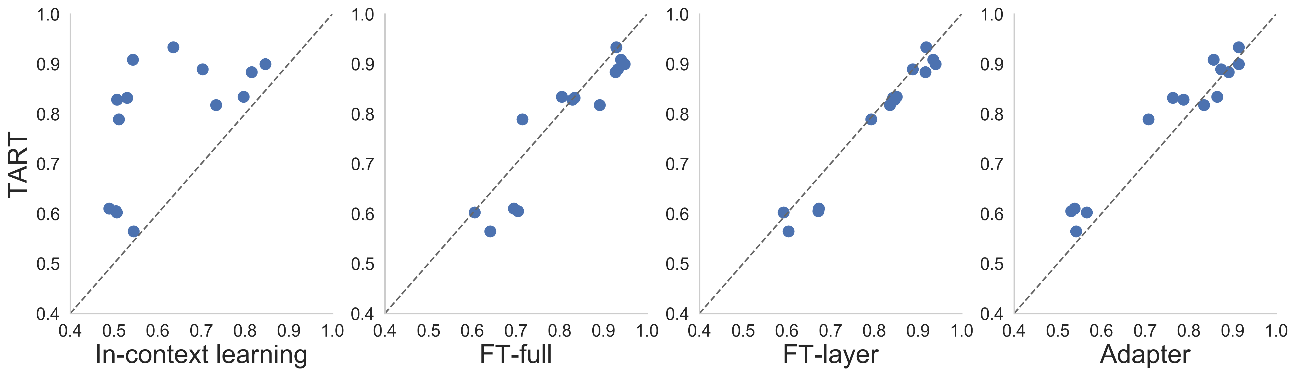
(c) Number of examples = 48

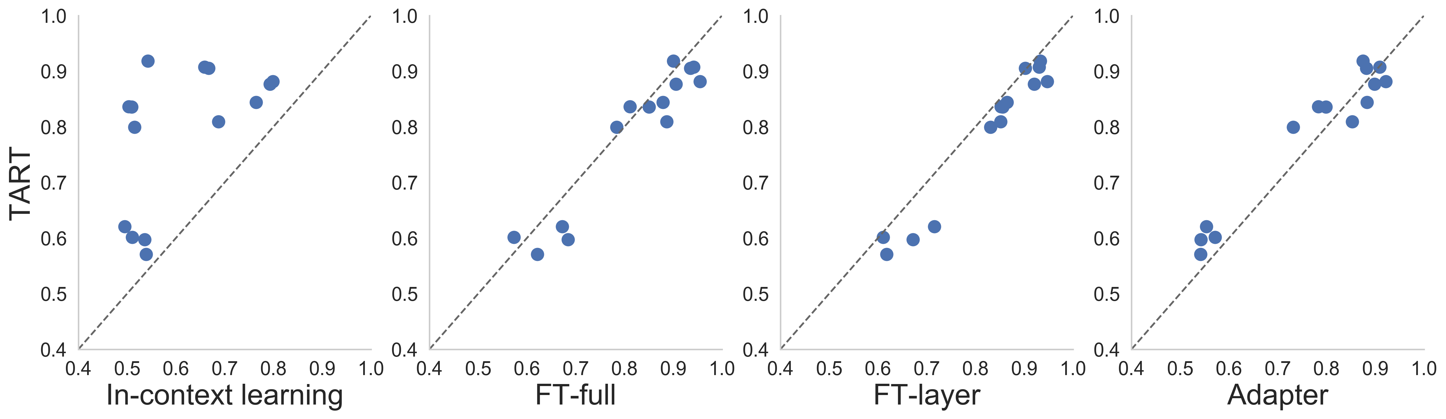
(d) Number of examples = 64

Figure 23: Comparison of Tart and task-adaptation approaches (Bloom (560M)). We see that for Bloom (560M), Tart outperforms in-context learning and adapters and is competitive with full fine-tuning across all $k$.

D.1.2 Baseline methods

For each dataset, we compare Tart to 4 baseline task-adaptation methods: 1) in-context learning, 2) full fine-tuning, 3) last layer fine-tuning, and 4) adapters. The last layer fine-tuning and the adapters are trained as follows:

• Last layer fine-tuning: Freeze all layers of transformer but the final transformer block and the language modeling head.

• Adapter: Combine a frozen LLM base transformer model with a trainable adapter head—an MLP composed of a single linear layer followed by non-linearity.

Hyperparameter search.

For each baseline, we perform an extensive hyperparameter search over number of epochs and learning rate for each dataset in order to optimize performance. We search over a range of learning rates (1e-3, 1e-4, 3e-5, 1e-5, 8e-6), and range of epochs (5, 10, 15, 20, 50). For all models < 1B parameters, we use a batch size of 1. For all models > 1B parameters, we use a batch size of 8. We use these same batch sizes at evaluation time. We perform our hyperparameter searches with a fixed number of train samples (64). We run our hyperparameter searches over 3 random seeds.

D.2 NL benchmarks

In this section, we provide additional results deferred from Section 5 on the NLP benchmark evaluations, RAFT evaluations and demonstration of Tart’s data-scalability.

D.2.1 Performance on benchmark datasets

Figure 20 shows the performance of the baseline methods with Tart averaged across the suite of 14 datasets. Tart, while being task-agnostic, shows similar performance quality to task-specific approaches across the different model families, and consistently outperforms in-context learning.

Figures 21, 22, and 23 show the scatter plots of the accuracies of Tart with the baseline methods across datasets and different values of in-context examples $k$. An interesting observation is that as the number of examples $k$ increases from $18$ to $64$, the performance of fine-tuning improves at a better rate than that of Tart.

D.2.2 Real-world Annotated Few-shot Tasks (RAFT) evaluation

For our evaluations on the RAFT benchmark [Ale+21], we follow the protocol (same train and test sets) used in HELM benchmark. The HELM benchmark [Lia+22] contains the evaluation results for many open and closed models enabling us to accurately compare the performance of Tart with other models. We evaluate Tart on all RAFT binary classification datasets (twitter-complaints, neurips-impact-statement-risks, overulling, ade-corpusv2, tweet-eval-hate, terms-of-service, tai-safety-research) with the exception of systematic-review-inclusion which contains zero positive samples in the train set. Tart requires at least one example of each class in the training set. Table 1 contains a detailed performance comparison of Tart with respect to other models. Tart when combined with GPT-Neo (125M) is able to outperform Bloom (176B) and is competitive with OPT (175B) and GPT-3 (175B), all of which have 1000x more parameters.

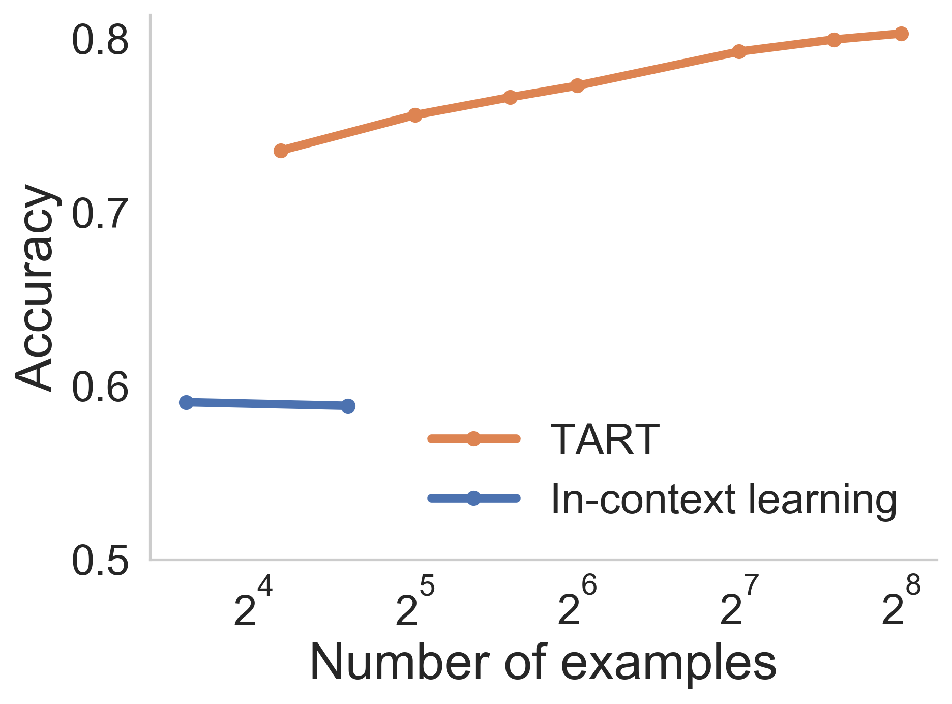
(a) GPT-Neo (125M)

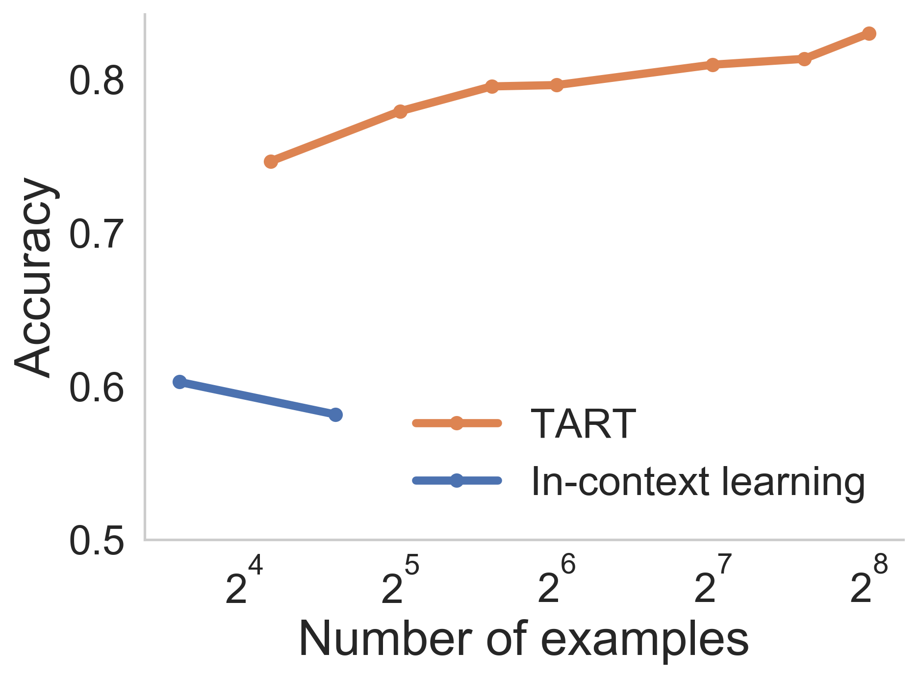
(b) Pythia (160M)

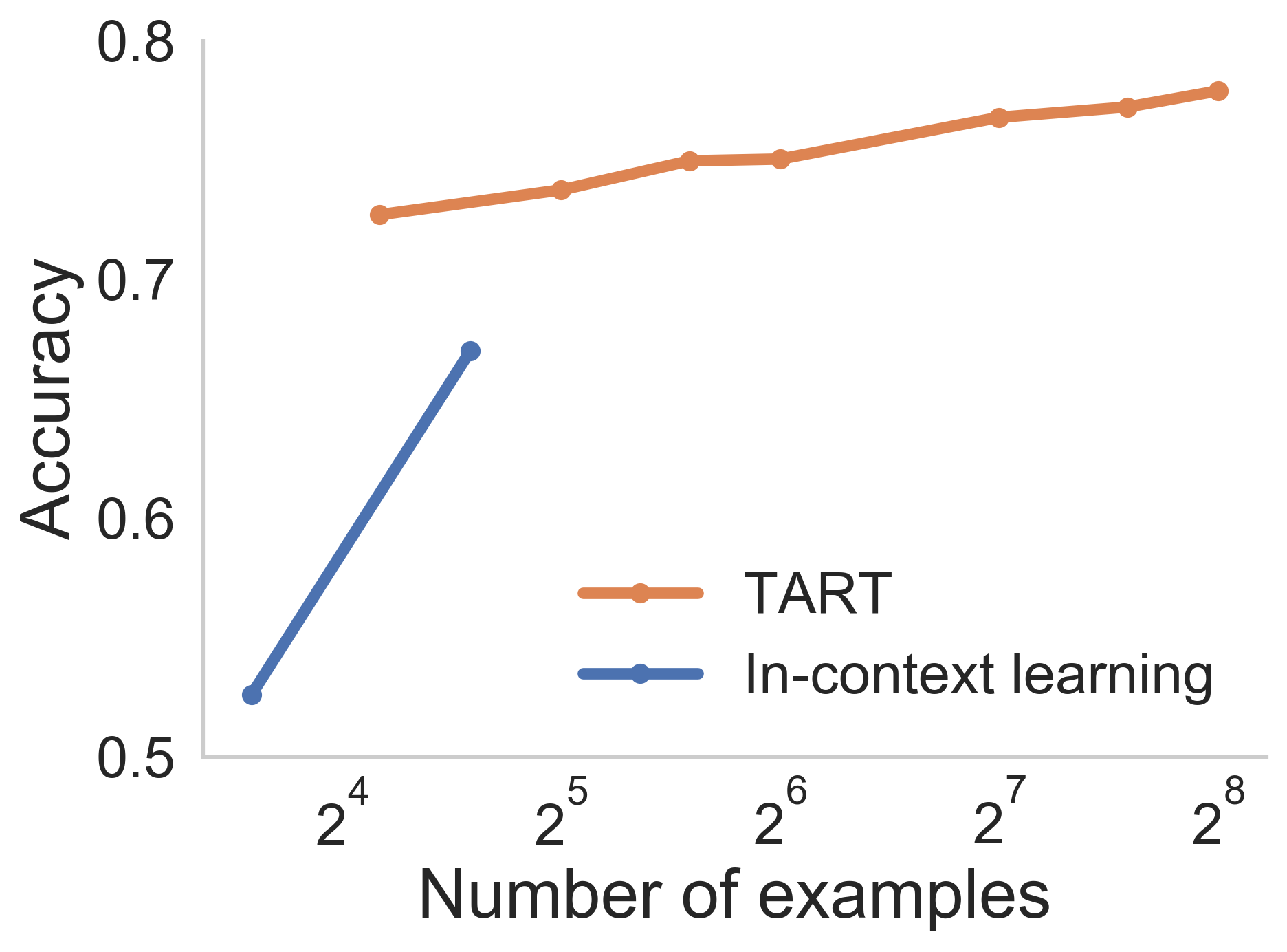
(c) Bloom (560M)

Figure 24: Beyond context window constraints. Performance comparison with respect to number of in-context examples. Base in-context learning is bound with respect to total numbers of examples and performance saturates. Tart is not bound by context length, and performance continues to scale as number of examples increases.

D.2.3 Beyond context length: Tart is data-scalable

Setup.

For these evaluations, we use the a subset of 6 datasets: AG-News-0, DBPedia-0, SST, SMS Spam, Youtube and Rotten Tomatoes. We evaluate the performance of Tart over $k$=[18, 32, 48, 64, 128, 192, 256] where $k$ is the number of in-context examples. When evaluating our base models, we evaluate over $k$=[8, 24]—values of $k$ that maximize the context window. We use a lower-bound of 8 given that the maximum input sequence length in the training set for AG News is 256. With such a sequence length, the maximum number of in-context examples that fit in the context-window is 8, hence the lower bound.

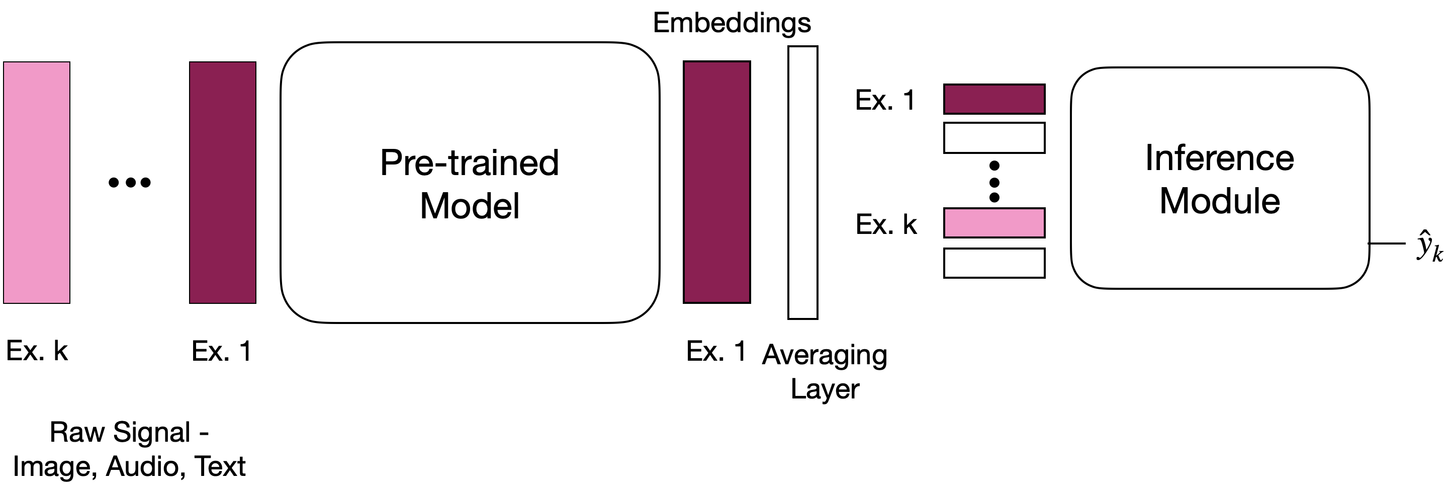
Figure 25: Stream embeddings. Another protocol for generating representations for in-context examples where each example is embedded by the base model separately.

Embeddings.

For these evaluations, we use what we call “streaming” embeddings (see Figure 25). In this setup, we use the context window of the LLM to encode a single example at a time. The final embeddings are then averaged and used in-context with Tart’s reasoning module. This is in contrast to the vanilla and LOO embeddings which use multiple examples in-context with the base LLM to obtain the embeddings.

Evaluation.

Figure 24 shows the performance of base in-context learning with Tart across the three different model families. Observe that while in-context learning is bottlenecked by the context window of the base LLM, Tart is able to learn from 10x more examples and exhibits an increasing trend in accuracy with number of examples across models.

D.3 Extension to other modalities: Tart is domain-agnostic!

We begin by providng a description of the datasets we used to evaluate Tart on audio and vision tasks, and then provide additional results comparing our algorithm with baselines.

D.3.1 Dataset details

For audio classification, we use the Speech Commands (Version 0.01) dataset [War18]. Speech Commands is a multi-class classification task where the task is to detect preregistered keywords by classifying utterances into a predefined set of words. We construct a 3 binary classification task over the keywords “stop” and “go”, “up” and “down”, and “yes” and “no” (see Table 4 for more details).

For image classification, we use CIFAR-10 [Kri09] and MNIST [LCB10]. Both tasks are multi-class classification tasks. We create 3 binary classification tasks for each of the datasets. For CIFAR-10 the tasks are: airplane vs. bird, bird vs. horse, and ship vs. automobile. For MNIST the tasks are: 0 vs. 8, 1 vs. 6 and 2 vs. 4. See Table 4 for more details.

For both the audio and image datasets, we sample a class-balanced set of 256 samples from the training set. For the test sets, we filter the original test sets to only include samples of the two classes we are learning to predict for (i.e., airplane and bird for CIFAR10 and 0 and 8 for MNIST).

Dataset	Modality	Train size	Test size
MNIST (0 vs. 8)	image	256	1954
MNIST (1 vs. 6)	image	256	2093
MNIST (2 vs. 4)	image	256	2014
Speech Commands (stop vs. go)	audio	256	500
Speech Commands (up vs. down)	audio	256	508
Speech Commands (yes vs. no)	audio	256	525
CIFAR-10 (airplane vs. bird)	image	256	2000
CIFAR-10 (bird vs. horse)	image	256	2000
CIFAR-10 (ship vs. automobile)	image	256	2000

Table 4: Dataset statistics for all audio and image evaluation datasets.

D.3.2 Algorithms for comparison

For these evaluations, we use the “streaming embeddings” described in Figure 25 to obtain the embedding for Tart. We evaluate over $k$=[18, 32, 48, 64, 128, 256].

We compare against two baseline task-adaptation methods: 1) full fine-tuning and 2) adapters. We use the same architectures as described in Appendix D.1.2. For vision tasks, we use Google’s 307M parameter pretrained Vision Transformer (ViT) model [Wu+20]: ViT-large-patch16-224-in21k. For audio tasks, we use OpenAI’s 1.5B parameter pretrained Whisper model [Rad+22]: Whisper-large.

Hyperparameter search

For each baseline, we perform an extensive hyperparameter search over number of epochs and learning rate for each dataset in order to optimize performance. We search over a range of learning rates (1e-3, 5e-04, 1e-4, 5e-5, 1e-5, and 8e-6) and a range of epochs (5, 10, 15 and 20). For all models we use a batch size of 1. We perform our hyperparameter searches for a fixed number of train samples (128) and run our hyperparameter searches over 3 random seeds.

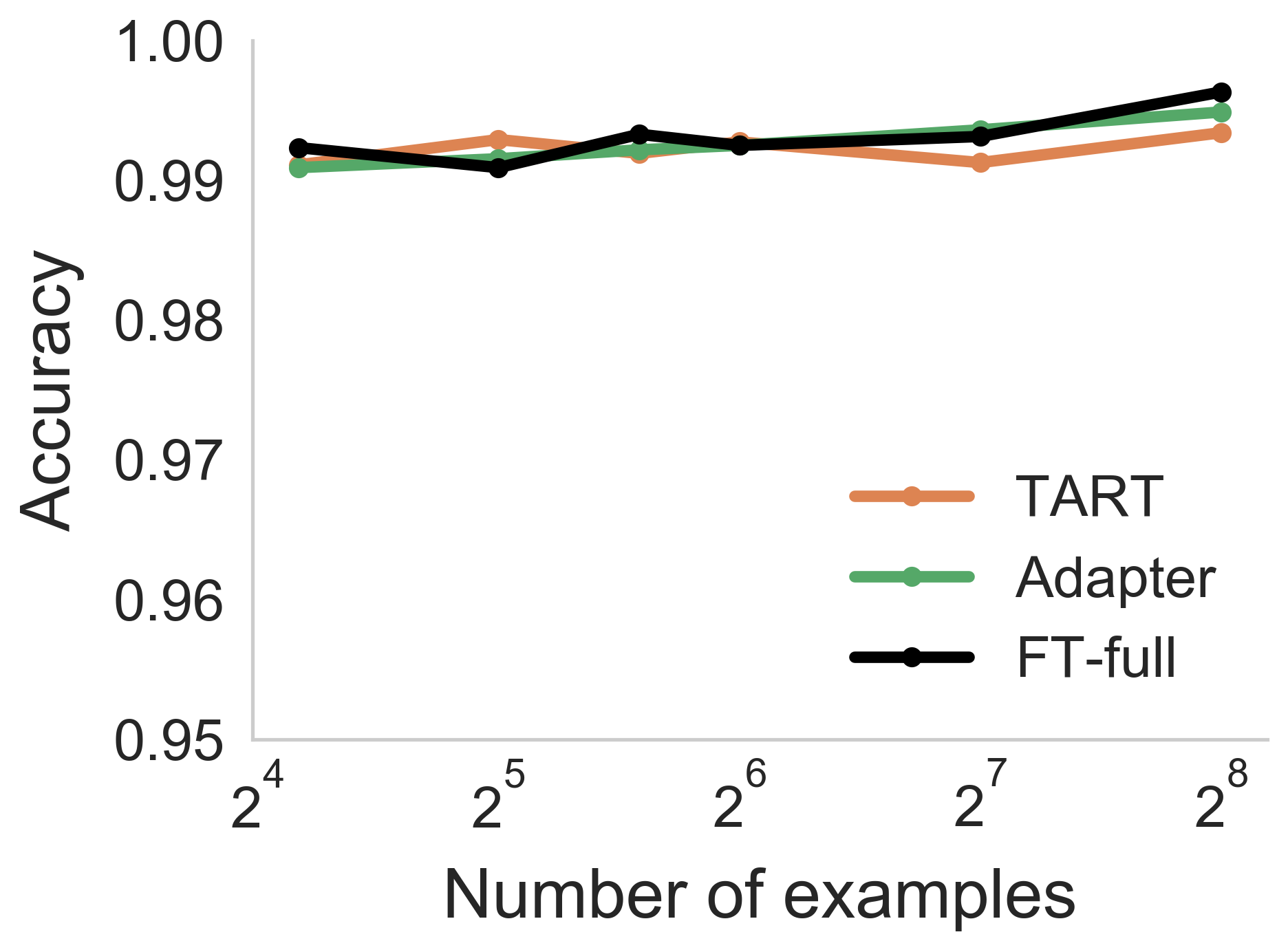
(a) MNIST (1 vs. 6)

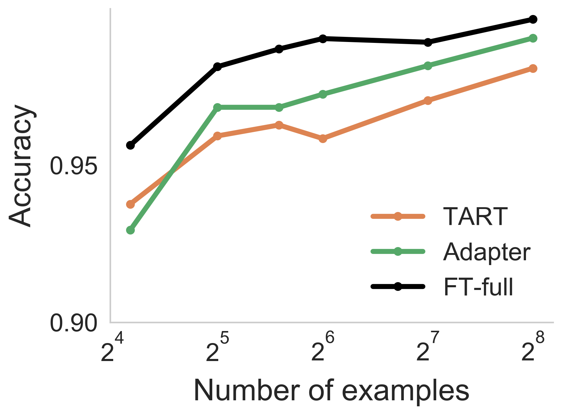
(b) MNIST (2 vs. 4)

Figure 26: Additional MNIST binary classification tasks. TART is competitive with task-specific full fine-tuning and adapters.

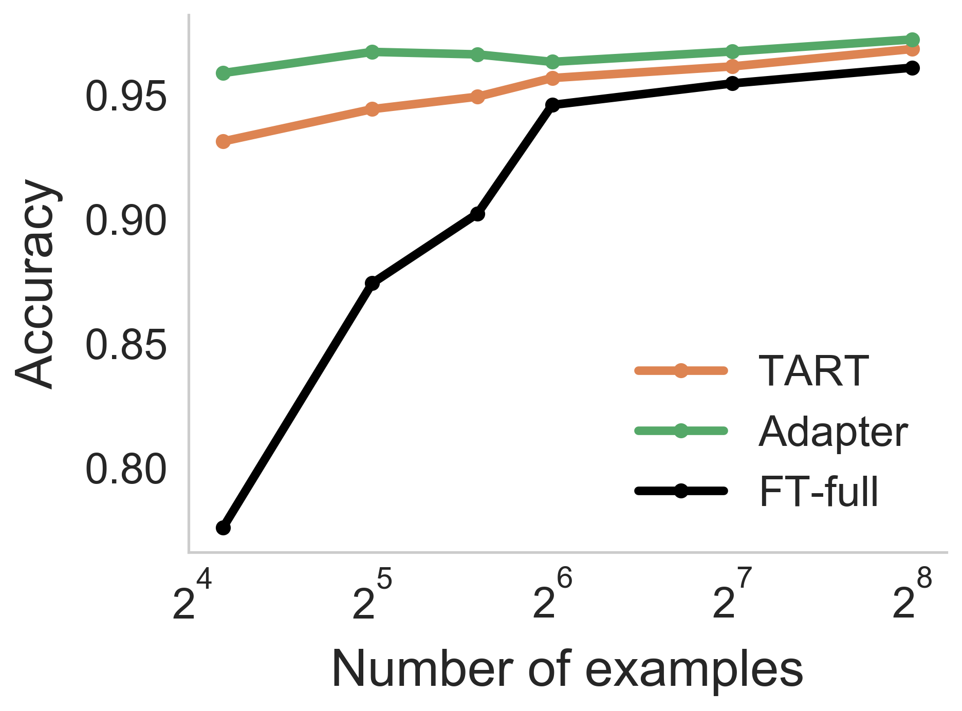
(a) CIFAR-10 (ship vs. automobile)

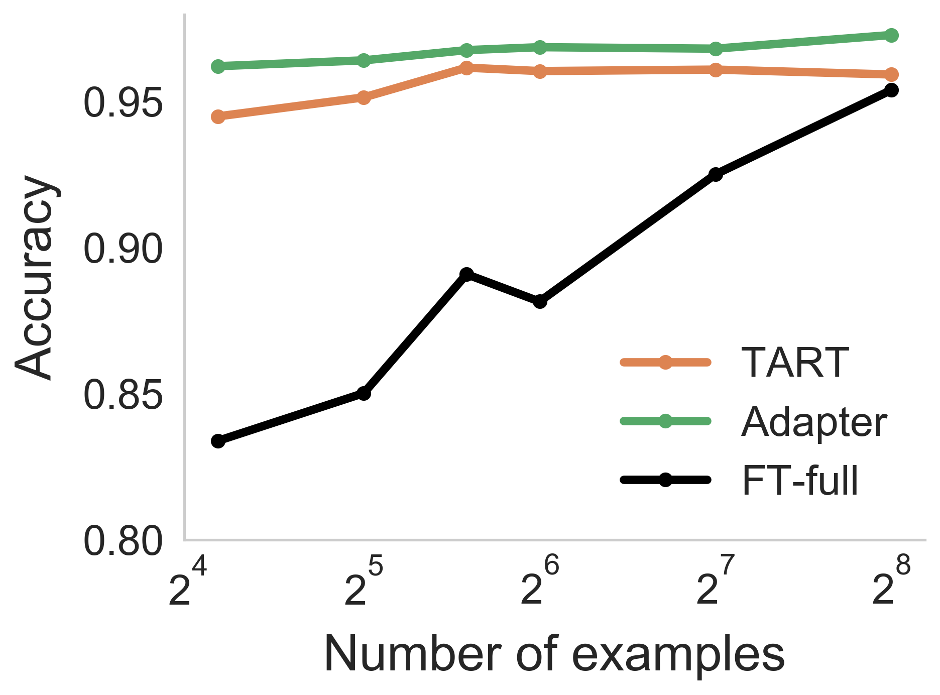
(b) CIFAR-10 (bird vs. horse)

Figure 27: Additional CIFAR-10 binary classification tasks. TART is competitive with task-specific full fine-tuning and adapters.

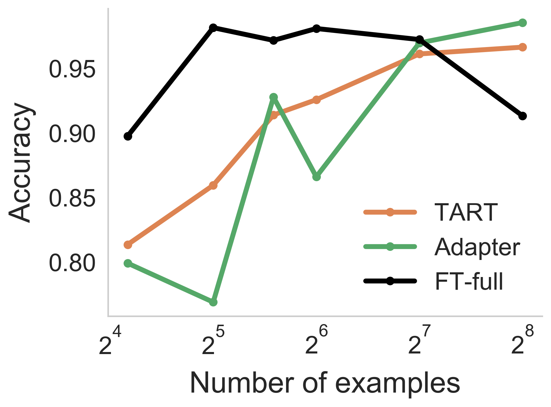
(a) Speech Commands (yes vs. no)

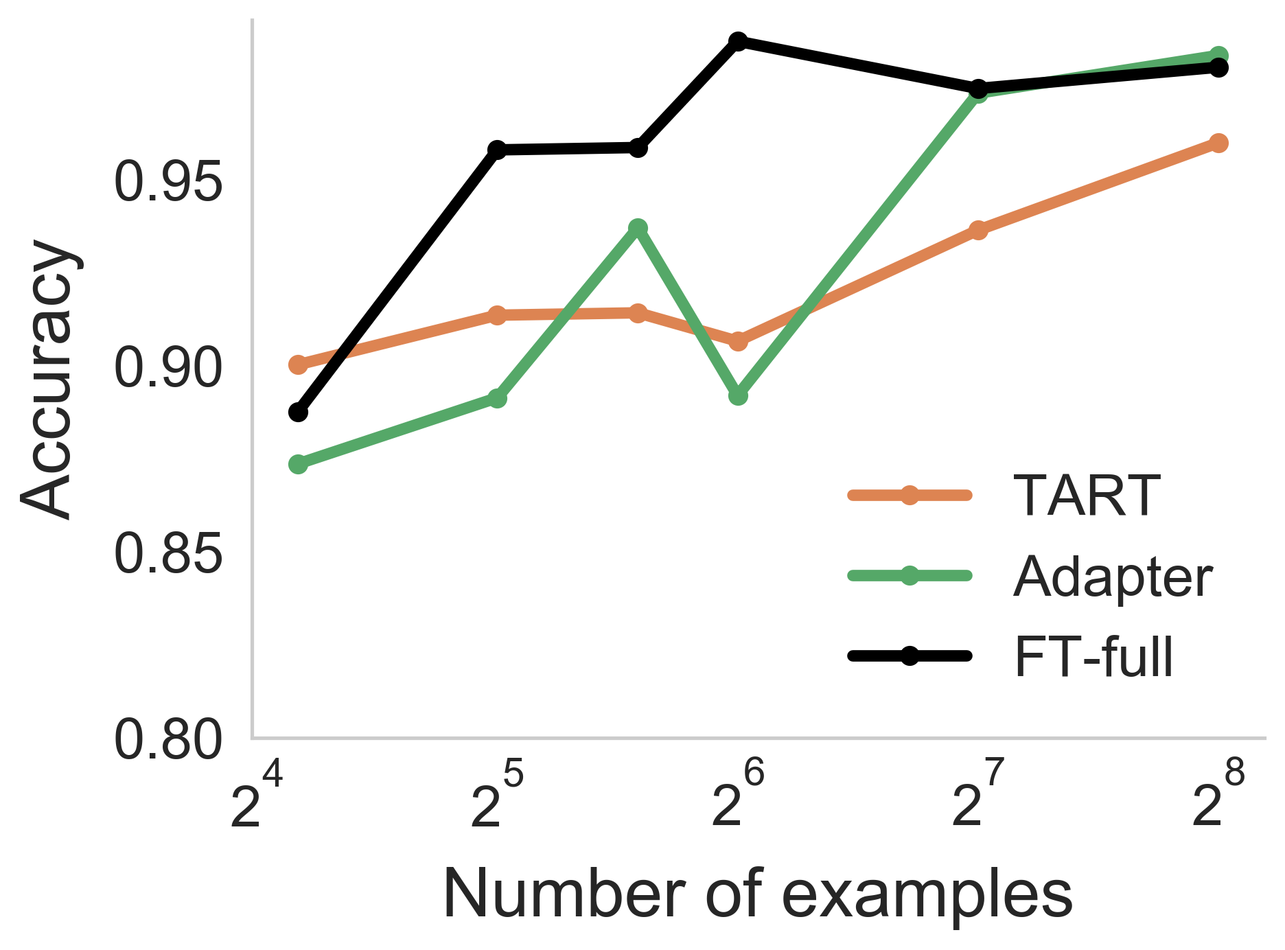
(b) Speech Commands (up vs. down)

Figure 28: Additional Speech Commands binary classification tasks. TART is competitive with task-specific full fine-tuning and adapters.

D.3.3 Evaluation

We plot the accuracy as a function of the number of examples for Tart, fine-tuning and adapter in Figure 26 (MNIST), Figure 27 (CIFAR-10), and Figure 28 (Speech Commands). Tart is competitive with both these baselines, showing how task-agnostic methods can compete with task-specific adaptation methods across different modalities.

D.4 Generalization across architectures

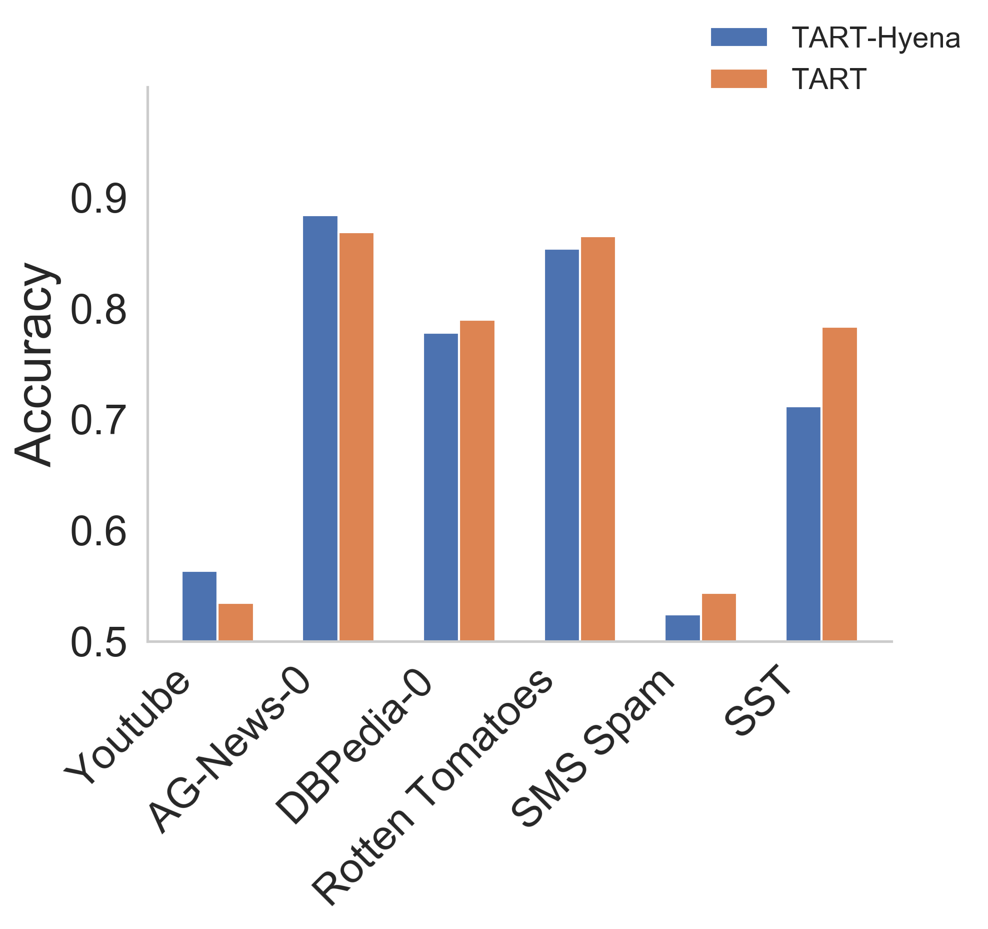
(a) k = 18

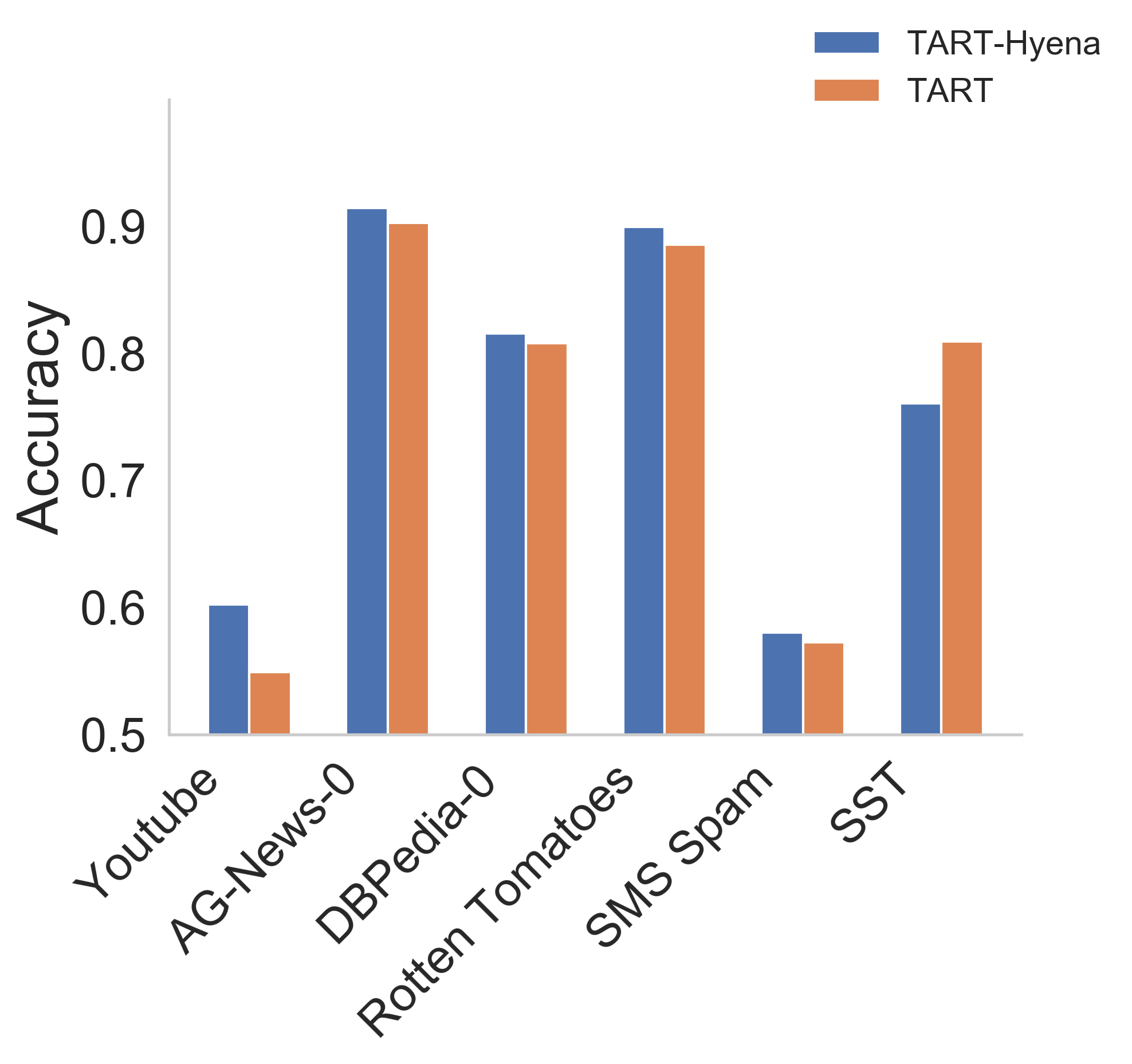
(b) k = 32

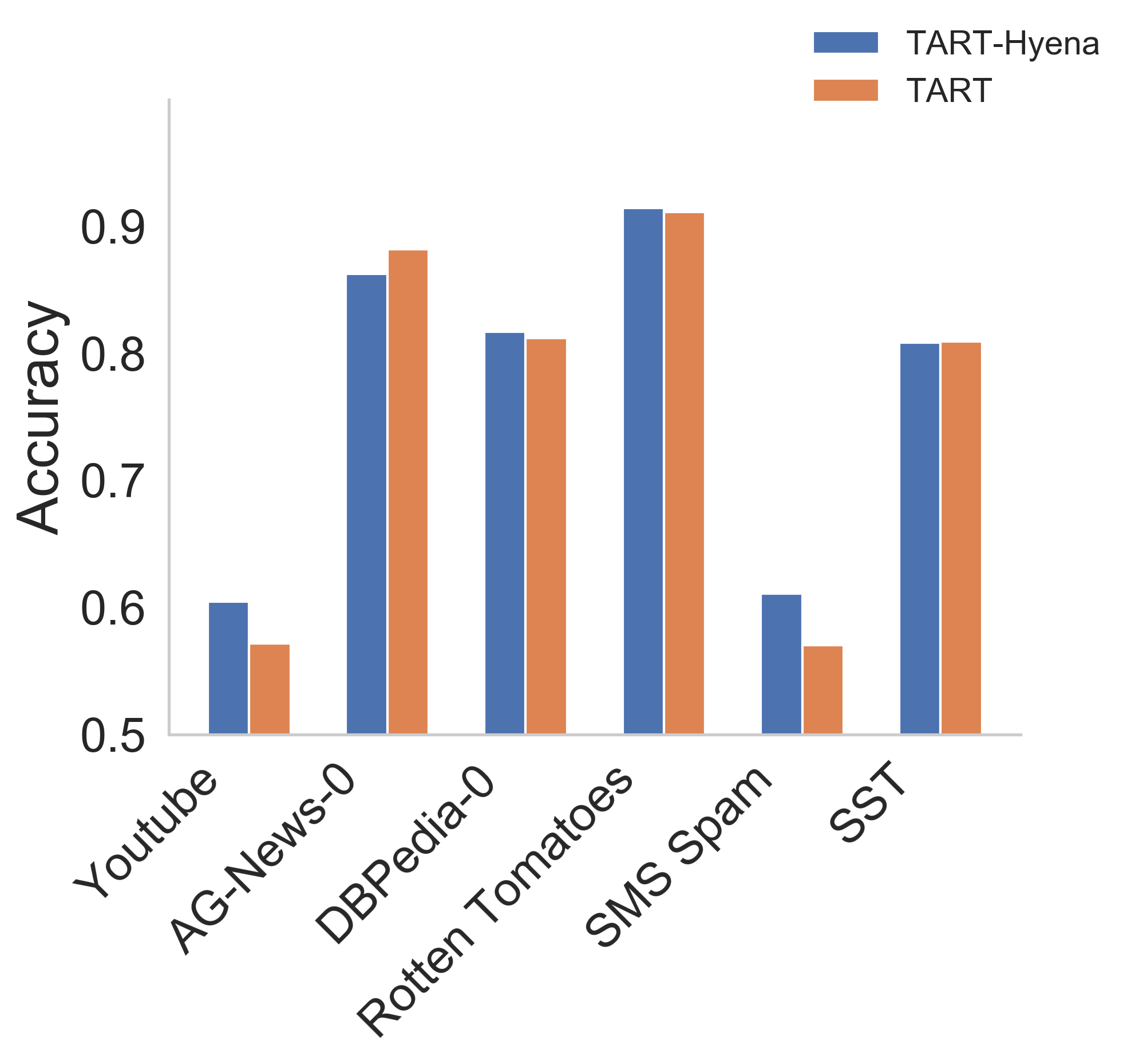
(c) k = 48

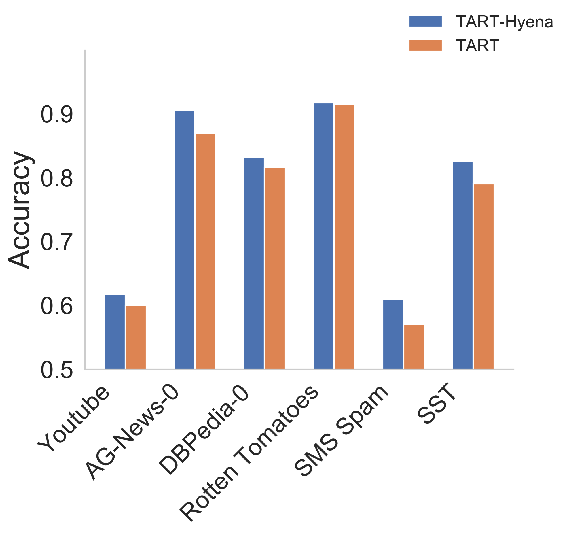
(d) k = 64

Figure 29: Comparing TART with a Hyena version of TART. Instead of using a Transformer module, we use a Hyena model to learn the probabilistic reasoning task. Hyena-TART is comparable to TART across datasets and achieves better performance for larger value of $k$ ($=64$).

In this section, we demonstrate that it is possible to train Tart reasoning modules on architectures beyond transformers. More concretely, we train a reasoning module that has the Hyena architecture [Pol+23] using the same synthetic logistic regression tasks.

D.4.1 Setup and Hyper-parameters

We instantiate a reasoning module with 12 Hyena blocks, a hidden dimension size of 256, and a sequence length of 2050. We train with a batch size of 16, using a learning rate of 5e-05. We sample data with a noise parameter ($\alpha$) equal to 1. We train the model for 5000 steps. For our evaluations, we use the final checkpoint (i.e., 5000) of the reasoning module.

D.4.2 Evaluation

We evaluate the Hyena-based reasoning module applied to GPT-Neo (125M) on 6 datasets: SMS Spam, SST, AG-News-0, DBpedia-14-0, Youtube, and Rotten Tomatoes. As seen in Figure 29, the Hyena-based reasoning module transfers to natural language tasks and performs competitively with the transformer-based reasoning module

Dataset	Tart	In-context learning	Fine-tuning full	Fine-tuning layer	Adapters
AG-News-0	0.790 $\pm$ 0.036	0.552 $\pm$ 0.049	0.724 $\pm$ 0.070	0.852 $\pm$ 0.019	0.824 $\pm$ 0.031
AG-News-1	0.828 $\pm$ 0.021	0.541 $\pm$ 0.037	0.779 $\pm$ 0.137	0.903 $\pm$ 0.021	0.868 $\pm$ 0.020
AG-News-2	0.751 $\pm$ 0.023	0.513 $\pm$ 0.014	0.626 $\pm$ 0.057	0.765 $\pm$ 0.025	0.755 $\pm$ 0.012
AG-News-3	0.743 $\pm$ 0.031	0.502 $\pm$ 0.017	0.736 $\pm$ 0.035	0.786 $\pm$ 0.025	0.727 $\pm$ 0.066
Civil Comments	0.559 $\pm$ 0.027	0.499 $\pm$ 0.002	0.520 $\pm$ 0.033	0.515 $\pm$ 0.019	0.555 $\pm$ 0.036
DBPedia-0	0.866 $\pm$ 0.030	0.611 $\pm$ 0.091	0.802 $\pm$ 0.020	0.825 $\pm$ 0.012	0.837 $\pm$ 0.022
DBPedia-1	0.778 $\pm$ 0.036	0.579 $\pm$ 0.100	0.766 $\pm$ 0.056	0.740 $\pm$ 0.041	0.778 $\pm$ 0.044
DBPedia-2	0.798 $\pm$ 0.042	0.609 $\pm$ 0.136	0.862 $\pm$ 0.041	0.908 $\pm$ 0.011	0.832 $\pm$ 0.048
DBPedia-3	0.812 $\pm$ 0.032	0.611 $\pm$ 0.135	0.817 $\pm$ 0.034	0.859 $\pm$ 0.025	0.848 $\pm$ 0.028
IMDB	0.537 $\pm$ 0.022	0.507 $\pm$ 0.007	0.625 $\pm$ 0.013	0.560 $\pm$ 0.021	0.556 $\pm$ 0.014
Rotten Tomatoes	0.535 $\pm$ 0.030	0.550 $\pm$ 0.043	0.689 $\pm$ 0.019	0.541 $\pm$ 0.037	0.524 $\pm$ 0.018
SMS Spam	0.869 $\pm$ 0.063	0.736 $\pm$ 0.099	0.925 $\pm$ 0.011	0.833 $\pm$ 0.015	0.886 $\pm$ 0.023
SST	0.544 $\pm$ 0.021	0.542 $\pm$ 0.024	0.715 $\pm$ 0.009	0.555 $\pm$ 0.026	0.547 $\pm$ 0.009
Youtube	0.784 $\pm$ 0.047	0.658 $\pm$ 0.089	0.833 $\pm$ 0.089	0.768 $\pm$ 0.100	0.715 $\pm$ 0.136

Table 5: Standard deviation of accuracy, number of examples = 18, GPT-Neo (125M)

Dataset	Tart	In-context learning	Fine-tuning full	Fine-tuning layer	Adapters
AG-News-0	0.805 $\pm$ 0.029	0.498 $\pm$ 0.002	0.758 $\pm$ 0.127	0.601 $\pm$ 0.072	0.669 $\pm$ 0.044
AG-News-1	0.825 $\pm$ 0.023	0.517 $\pm$ 0.019	0.916 $\pm$ 0.015	0.702 $\pm$ 0.097	0.690 $\pm$ 0.034
AG-News-2	0.758 $\pm$ 0.027	0.500 $\pm$ 0.000	0.596 $\pm$ 0.031	0.500 $\pm$ 0.001	0.588 $\pm$ 0.026
AG-News-3	0.754 $\pm$ 0.033	0.501 $\pm$ 0.003	0.661 $\pm$ 0.093	0.552 $\pm$ 0.041	0.613 $\pm$ 0.022
Civil Comments	0.575 $\pm$ 0.019	0.500 $\pm$ 0.003	0.525 $\pm$ 0.049	0.500 $\pm$ 0.000	0.515 $\pm$ 0.008
DBPedia-0	0.861 $\pm$ 0.018	0.508 $\pm$ 0.016	0.786 $\pm$ 0.054	0.638 $\pm$ 0.109	0.704 $\pm$ 0.038
DBPedia-1	0.813 $\pm$ 0.020	0.499 $\pm$ 0.010	0.787 $\pm$ 0.067	0.599 $\pm$ 0.078	0.710 $\pm$ 0.059
DBPedia-2	0.870 $\pm$ 0.035	0.502 $\pm$ 0.025	0.878 $\pm$ 0.071	0.701 $\pm$ 0.113	0.767 $\pm$ 0.052
DBPedia-3	0.850 $\pm$ 0.050	0.502 $\pm$ 0.003	0.864 $\pm$ 0.034	0.603 $\pm$ 0.114	0.734 $\pm$ 0.030
IMDB	0.550 $\pm$ 0.027	0.507 $\pm$ 0.005	0.590 $\pm$ 0.046	0.500 $\pm$ 0.000	0.526 $\pm$ 0.012
Rotten Tomatoes	0.544 $\pm$ 0.027	0.491 $\pm$ 0.013	0.589 $\pm$ 0.074	0.500 $\pm$ 0.000	0.522 $\pm$ 0.023
SMS Spam	0.901 $\pm$ 0.038	0.867 $\pm$ 0.030	0.892 $\pm$ 0.052	0.867 $\pm$ 0.004	0.851 $\pm$ 0.042
SST	0.572 $\pm$ 0.016	0.517 $\pm$ 0.002	0.617 $\pm$ 0.074	0.517 $\pm$ 0.000	0.539 $\pm$ 0.007
Youtube	0.847 $\pm$ 0.047	0.611 $\pm$ 0.084	0.810 $\pm$ 0.060	0.528 $\pm$ 0.000	0.598 $\pm$ 0.103

Table 6: Standard deviation of accuracy, number of examples = 18, Pythia (160M)

Dataset	Tart	In-context learning	Fine-tuning full	Fine-tuning layer	Adapters
AG-News-0	0.813 $\pm$ 0.021	0.511 $\pm$ 0.013	0.702 $\pm$ 0.102	0.790 $\pm$ 0.033	0.689 $\pm$ 0.060
AG-News-1	0.851 $\pm$ 0.020	0.511 $\pm$ 0.014	0.801 $\pm$ 0.086	0.891 $\pm$ 0.037	0.752 $\pm$ 0.032
AG-News-2	0.744 $\pm$ 0.034	0.509 $\pm$ 0.009	0.622 $\pm$ 0.083	0.711 $\pm$ 0.070	0.652 $\pm$ 0.047
AG-News-3	0.763 $\pm$ 0.026	0.508 $\pm$ 0.014	0.626 $\pm$ 0.016	0.775 $\pm$ 0.035	0.706 $\pm$ 0.027
Civil Comments	0.561 $\pm$ 0.029	0.489 $\pm$ 0.009	0.491 $\pm$ 0.032	0.540 $\pm$ 0.029	0.533 $\pm$ 0.030
DBPedia-0	0.851 $\pm$ 0.009	0.531 $\pm$ 0.044	0.811 $\pm$ 0.116	0.813 $\pm$ 0.057	0.812 $\pm$ 0.043
DBPedia-1	0.760 $\pm$ 0.037	0.546 $\pm$ 0.088	0.750 $\pm$ 0.129	0.718 $\pm$ 0.067	0.754 $\pm$ 0.041
DBPedia-2	0.800 $\pm$ 0.032	0.567 $\pm$ 0.110	0.850 $\pm$ 0.086	0.904 $\pm$ 0.018	0.851 $\pm$ 0.055
DBPedia-3	0.848 $\pm$ 0.025	0.528 $\pm$ 0.046	0.739 $\pm$ 0.133	0.785 $\pm$ 0.132	0.849 $\pm$ 0.011
IMDB	0.552 $\pm$ 0.031	0.550 $\pm$ 0.044	0.630 $\pm$ 0.016	0.608 $\pm$ 0.014	0.526 $\pm$ 0.025
Rotten Tomatoes	0.574 $\pm$ 0.029	0.539 $\pm$ 0.031	0.638 $\pm$ 0.037	0.618 $\pm$ 0.049	0.507 $\pm$ 0.010
SMS Spam	0.830 $\pm$ 0.112	0.613 $\pm$ 0.261	0.883 $\pm$ 0.130	0.911 $\pm$ 0.035	0.885 $\pm$ 0.045
SST	0.574 $\pm$ 0.019	0.561 $\pm$ 0.062	0.707 $\pm$ 0.024	0.636 $\pm$ 0.025	0.531 $\pm$ 0.015
Youtube	0.762 $\pm$ 0.116	0.584 $\pm$ 0.144	0.753 $\pm$ 0.140	0.726 $\pm$ 0.052	0.769 $\pm$ 0.084

Table 7: Standard deviation of accuracy, number of examples = 18, Bloom (560M)

Dataset	Tart	In-context learning	Fine-tuning full	Fine-tuning layer	Adapters
AG-News-0	0.808 $\pm$ 0.030	0.551 $\pm$ 0.041	0.795 $\pm$ 0.049	0.874 $\pm$ 0.022	0.830 $\pm$ 0.034
AG-News-1	0.883 $\pm$ 0.014	0.577 $\pm$ 0.055	0.852 $\pm$ 0.070	0.911 $\pm$ 0.021	0.902 $\pm$ 0.011
AG-News-2	0.764 $\pm$ 0.019	0.540 $\pm$ 0.027	0.705 $\pm$ 0.063	0.812 $\pm$ 0.019	0.782 $\pm$ 0.019
AG-News-3	0.798 $\pm$ 0.025	0.521 $\pm$ 0.039	0.762 $\pm$ 0.046	0.813 $\pm$ 0.012	0.806 $\pm$ 0.028
Civil Comments	0.575 $\pm$ 0.054	0.498 $\pm$ 0.002	0.554 $\pm$ 0.029	0.543 $\pm$ 0.022	0.579 $\pm$ 0.044
DBPedia-0	0.886 $\pm$ 0.021	0.632 $\pm$ 0.096	0.884 $\pm$ 0.019	0.866 $\pm$ 0.013	0.859 $\pm$ 0.020
DBPedia-1	0.809 $\pm$ 0.031	0.593 $\pm$ 0.062	0.802 $\pm$ 0.030	0.783 $\pm$ 0.022	0.813 $\pm$ 0.023
DBPedia-2	0.886 $\pm$ 0.011	0.586 $\pm$ 0.078	0.916 $\pm$ 0.029	0.932 $\pm$ 0.013	0.899 $\pm$ 0.017
DBPedia-3	0.868 $\pm$ 0.022	0.565 $\pm$ 0.041	0.902 $\pm$ 0.016	0.908 $\pm$ 0.012	0.868 $\pm$ 0.023
IMDB	0.537 $\pm$ 0.040	0.543 $\pm$ 0.029	0.609 $\pm$ 0.029	0.556 $\pm$ 0.024	0.551 $\pm$ 0.036
Rotten Tomatoes	0.549 $\pm$ 0.035	0.554 $\pm$ 0.036	0.667 $\pm$ 0.036	0.550 $\pm$ 0.045	0.528 $\pm$ 0.020
SMS Spam	0.903 $\pm$ 0.027	0.768 $\pm$ 0.105	0.931 $\pm$ 0.014	0.861 $\pm$ 0.027	0.920 $\pm$ 0.011
SST	0.573 $\pm$ 0.009	0.564 $\pm$ 0.045	0.711 $\pm$ 0.022	0.594 $\pm$ 0.022	0.551 $\pm$ 0.022
Youtube	0.810 $\pm$ 0.072	0.759 $\pm$ 0.074	0.854 $\pm$ 0.044	0.773 $\pm$ 0.052	0.722 $\pm$ 0.113

Table 8: Standard deviation of accuracy, number of examples = 32, GPT-Neo (125M)

Dataset	Tart	In-context learning	Fine-tuning full	Fine-tuning layer	Adapters
AG-News-0	0.835 $\pm$ 0.020	0.499 $\pm$ 0.002	0.791 $\pm$ 0.100	0.855 $\pm$ 0.017	0.712 $\pm$ 0.028
AG-News-1	0.900 $\pm$ 0.012	0.504 $\pm$ 0.004	0.911 $\pm$ 0.022	0.926 $\pm$ 0.009	0.738 $\pm$ 0.028
AG-News-2	0.773 $\pm$ 0.012	0.510 $\pm$ 0.006	0.687 $\pm$ 0.034	0.742 $\pm$ 0.044	0.683 $\pm$ 0.025
AG-News-3	0.823 $\pm$ 0.024	0.514 $\pm$ 0.017	0.792 $\pm$ 0.022	0.833 $\pm$ 0.011	0.697 $\pm$ 0.023
Civil Comments	0.596 $\pm$ 0.024	0.499 $\pm$ 0.007	0.588 $\pm$ 0.052	0.536 $\pm$ 0.020	0.542 $\pm$ 0.016
DBPedia-0	0.890 $\pm$ 0.016	0.514 $\pm$ 0.026	0.880 $\pm$ 0.049	0.777 $\pm$ 0.055	0.782 $\pm$ 0.044
DBPedia-1	0.833 $\pm$ 0.018	0.522 $\pm$ 0.023	0.834 $\pm$ 0.061	0.768 $\pm$ 0.024	0.760 $\pm$ 0.022
DBPedia-2	0.912 $\pm$ 0.010	0.522 $\pm$ 0.031	0.916 $\pm$ 0.033	0.903 $\pm$ 0.012	0.859 $\pm$ 0.019
DBPedia-3	0.879 $\pm$ 0.021	0.520 $\pm$ 0.026	0.900 $\pm$ 0.019	0.863 $\pm$ 0.018	0.812 $\pm$ 0.022
IMDB	0.541 $\pm$ 0.041	0.510 $\pm$ 0.008	0.630 $\pm$ 0.017	0.575 $\pm$ 0.024	0.540 $\pm$ 0.018
Rotten Tomatoes	0.576 $\pm$ 0.042	0.495 $\pm$ 0.007	0.659 $\pm$ 0.064	0.568 $\pm$ 0.027	0.542 $\pm$ 0.019
SMS Spam	0.937 $\pm$ 0.017	0.856 $\pm$ 0.080	0.913 $\pm$ 0.044	0.953 $\pm$ 0.014	0.877 $\pm$ 0.036
SST	0.602 $\pm$ 0.015	0.509 $\pm$ 0.013	0.705 $\pm$ 0.021	0.605 $\pm$ 0.043	0.542 $\pm$ 0.003
Youtube	0.862 $\pm$ 0.045	0.626 $\pm$ 0.081	0.874 $\pm$ 0.046	0.762 $\pm$ 0.052	0.654 $\pm$ 0.050

Table 9: Standard deviation of accuracy, number of examples = 32, Pythia (160M)

Dataset	Tart	In-context learning	Fine-tuning full	Fine-tuning layer	Adapters
AG-News-0	0.825 $\pm$ 0.031	0.503 $\pm$ 0.003	0.802 $\pm$ 0.041	0.818 $\pm$ 0.014	0.739 $\pm$ 0.049
AG-News-1	0.880 $\pm$ 0.012	0.516 $\pm$ 0.026	0.898 $\pm$ 0.043	0.912 $\pm$ 0.034	0.829 $\pm$ 0.010
AG-News-2	0.771 $\pm$ 0.009	0.519 $\pm$ 0.025	0.736 $\pm$ 0.071	0.773 $\pm$ 0.039	0.684 $\pm$ 0.040
AG-News-3	0.810 $\pm$ 0.016	0.509 $\pm$ 0.013	0.753 $\pm$ 0.058	0.805 $\pm$ 0.031	0.742 $\pm$ 0.030
Civil Comments	0.587 $\pm$ 0.025	0.500 $\pm$ 0.011	0.549 $\pm$ 0.016	0.564 $\pm$ 0.062	0.555 $\pm$ 0.009
DBPedia-0	0.857 $\pm$ 0.035	0.592 $\pm$ 0.083	0.801 $\pm$ 0.125	0.822 $\pm$ 0.043	0.834 $\pm$ 0.038
DBPedia-1	0.802 $\pm$ 0.031	0.558 $\pm$ 0.047	0.870 $\pm$ 0.037	0.800 $\pm$ 0.041	0.813 $\pm$ 0.034
DBPedia-2	0.879 $\pm$ 0.018	0.609 $\pm$ 0.025	0.938 $\pm$ 0.018	0.920 $\pm$ 0.031	0.903 $\pm$ 0.021
DBPedia-3	0.866 $\pm$ 0.035	0.634 $\pm$ 0.110	0.812 $\pm$ 0.163	0.911 $\pm$ 0.004	0.876 $\pm$ 0.037
IMDB	0.553 $\pm$ 0.046	0.541 $\pm$ 0.024	0.636 $\pm$ 0.016	0.600 $\pm$ 0.018	0.536 $\pm$ 0.024
Rotten Tomatoes	0.589 $\pm$ 0.037	0.575 $\pm$ 0.039	0.713 $\pm$ 0.029	0.630 $\pm$ 0.026	0.527 $\pm$ 0.015
SMS Spam	0.933 $\pm$ 0.017	0.762 $\pm$ 0.033	0.956 $\pm$ 0.026	0.905 $\pm$ 0.056	0.917 $\pm$ 0.017
SST	0.579 $\pm$ 0.032	0.502 $\pm$ 0.020	0.739 $\pm$ 0.013	0.638 $\pm$ 0.035	0.562 $\pm$ 0.017
Youtube	0.799 $\pm$ 0.117	0.710 $\pm$ 0.182	0.887 $\pm$ 0.033	0.756 $\pm$ 0.115	0.850 $\pm$ 0.024

Table 10: Standard deviation of accuracy, number of examples = 32, Bloom (560M)

Dataset	Tart	In-context learning	Fine-tuning full	Fine-tuning layer	Adapters
AG-News-0	0.812 $\pm$ 0.021	0.560 $\pm$ 0.046	0.832 $\pm$ 0.023	0.876 $\pm$ 0.012	0.833 $\pm$ 0.016
AG-News-1	0.904 $\pm$ 0.009	0.623 $\pm$ 0.051	0.924 $\pm$ 0.026	0.932 $\pm$ 0.007	0.923 $\pm$ 0.009
AG-News-2	0.786 $\pm$ 0.008	0.566 $\pm$ 0.023	0.791 $\pm$ 0.016	0.824 $\pm$ 0.010	0.797 $\pm$ 0.010
AG-News-3	0.822 $\pm$ 0.030	0.533 $\pm$ 0.029	0.800 $\pm$ 0.042	0.840 $\pm$ 0.015	0.825 $\pm$ 0.034
Civil Comments	0.591 $\pm$ 0.029	0.497 $\pm$ 0.003	0.568 $\pm$ 0.038	0.554 $\pm$ 0.029	0.614 $\pm$ 0.028
DBPedia-0	0.911 $\pm$ 0.011	0.676 $\pm$ 0.097	0.892 $\pm$ 0.017	0.898 $\pm$ 0.012	0.894 $\pm$ 0.023
DBPedia-1	0.823 $\pm$ 0.025	0.644 $\pm$ 0.115	0.838 $\pm$ 0.058	0.819 $\pm$ 0.018	0.833 $\pm$ 0.026
DBPedia-2	0.902 $\pm$ 0.015	0.622 $\pm$ 0.114	0.931 $\pm$ 0.032	0.940 $\pm$ 0.005	0.913 $\pm$ 0.007
DBPedia-3	0.883 $\pm$ 0.023	0.620 $\pm$ 0.129	0.891 $\pm$ 0.015	0.911 $\pm$ 0.006	0.889 $\pm$ 0.021
IMDB	0.557 $\pm$ 0.033	0.522 $\pm$ 0.025	0.641 $\pm$ 0.008	0.564 $\pm$ 0.017	0.577 $\pm$ 0.020
Rotten Tomatoes	0.572 $\pm$ 0.014	0.548 $\pm$ 0.045	0.710 $\pm$ 0.010	0.575 $\pm$ 0.048	0.572 $\pm$ 0.029
SMS Spam	0.882 $\pm$ 0.044	0.860 $\pm$ 0.036	0.946 $\pm$ 0.019	0.881 $\pm$ 0.013	0.925 $\pm$ 0.010
SST	0.570 $\pm$ 0.019	0.563 $\pm$ 0.032	0.705 $\pm$ 0.019	0.575 $\pm$ 0.028	0.542 $\pm$ 0.035
Youtube	0.810 $\pm$ 0.039	0.792 $\pm$ 0.081	0.923 $\pm$ 0.014	0.874 $\pm$ 0.029	0.832 $\pm$ 0.053

Table 11: Standard deviation of accuracy, number of examples = 48, GPT-Neo (125M)

Dataset	Tart	In-context learning	Fine-tuning full	Fine-tuning layer	Adapters
AG-News-0	0.846 $\pm$ 0.018	0.496 $\pm$ 0.007	0.871 $\pm$ 0.015	0.871 $\pm$ 0.005	0.732 $\pm$ 0.036
AG-News-1	0.923 $\pm$ 0.005	0.528 $\pm$ 0.044	0.942 $\pm$ 0.004	0.935 $\pm$ 0.009	0.780 $\pm$ 0.040
AG-News-2	0.798 $\pm$ 0.009	0.509 $\pm$ 0.004	0.731 $\pm$ 0.040	0.782 $\pm$ 0.018	0.722 $\pm$ 0.019
AG-News-3	0.845 $\pm$ 0.012	0.515 $\pm$ 0.014	0.787 $\pm$ 0.046	0.852 $\pm$ 0.011	0.718 $\pm$ 0.026
Civil Comments	0.605 $\pm$ 0.037	0.512 $\pm$ 0.009	0.607 $\pm$ 0.039	0.556 $\pm$ 0.014	0.556 $\pm$ 0.018
DBPedia-0	0.905 $\pm$ 0.020	0.549 $\pm$ 0.057	0.924 $\pm$ 0.020	0.830 $\pm$ 0.034	0.798 $\pm$ 0.021
DBPedia-1	0.840 $\pm$ 0.021	0.592 $\pm$ 0.062	0.867 $\pm$ 0.024	0.808 $\pm$ 0.031	0.780 $\pm$ 0.011
DBPedia-2	0.916 $\pm$ 0.009	0.636 $\pm$ 0.081	0.937 $\pm$ 0.017	0.923 $\pm$ 0.013	0.870 $\pm$ 0.022
DBPedia-3	0.888 $\pm$ 0.022	0.618 $\pm$ 0.096	0.927 $\pm$ 0.011	0.885 $\pm$ 0.007	0.827 $\pm$ 0.026
IMDB	0.557 $\pm$ 0.034	0.503 $\pm$ 0.008	0.632 $\pm$ 0.013	0.566 $\pm$ 0.030	0.545 $\pm$ 0.008
Rotten Tomatoes	0.601 $\pm$ 0.026	0.480 $\pm$ 0.014	0.683 $\pm$ 0.033	0.556 $\pm$ 0.033	0.562 $\pm$ 0.018
SMS Spam	0.956 $\pm$ 0.008	0.869 $\pm$ 0.044	0.966 $\pm$ 0.011	0.960 $\pm$ 0.008	0.891 $\pm$ 0.035
SST	0.612 $\pm$ 0.024	0.500 $\pm$ 0.025	0.702 $\pm$ 0.046	0.594 $\pm$ 0.042	0.560 $\pm$ 0.023
Youtube	0.872 $\pm$ 0.019	0.654 $\pm$ 0.063	0.904 $\pm$ 0.033	0.826 $\pm$ 0.046	0.666 $\pm$ 0.027

Table 12: Standard deviation of accuracy, number of examples = 48, Pythia (160M)

Dataset	Tart	In-context learning	Fine-tuning full	Fine-tuning layer	Adapters
AG-News-0	0.829 $\pm$ 0.029	0.507 $\pm$ 0.005	0.829 $\pm$ 0.071	0.847 $\pm$ 0.022	0.788 $\pm$ 0.028
AG-News-1	0.909 $\pm$ 0.010	0.543 $\pm$ 0.052	0.940 $\pm$ 0.011	0.935 $\pm$ 0.004	0.856 $\pm$ 0.014
AG-News-2	0.789 $\pm$ 0.016	0.511 $\pm$ 0.012	0.715 $\pm$ 0.057	0.793 $\pm$ 0.027	0.708 $\pm$ 0.011
AG-News-3	0.832 $\pm$ 0.018	0.530 $\pm$ 0.038	0.834 $\pm$ 0.029	0.843 $\pm$ 0.014	0.763 $\pm$ 0.015
Civil Comments	0.602 $\pm$ 0.030	0.506 $\pm$ 0.011	0.605 $\pm$ 0.044	0.592 $\pm$ 0.039	0.566 $\pm$ 0.008
DBPedia-0	0.889 $\pm$ 0.022	0.703 $\pm$ 0.085	0.933 $\pm$ 0.021	0.888 $\pm$ 0.024	0.873 $\pm$ 0.027
DBPedia-1	0.817 $\pm$ 0.023	0.734 $\pm$ 0.076	0.891 $\pm$ 0.028	0.836 $\pm$ 0.036	0.834 $\pm$ 0.024
DBPedia-2	0.900 $\pm$ 0.011	0.847 $\pm$ 0.037	0.949 $\pm$ 0.013	0.940 $\pm$ 0.009	0.914 $\pm$ 0.013
DBPedia-3	0.884 $\pm$ 0.020	0.815 $\pm$ 0.105	0.928 $\pm$ 0.024	0.917 $\pm$ 0.015	0.891 $\pm$ 0.037
IMDB	0.565 $\pm$ 0.033	0.545 $\pm$ 0.033	0.641 $\pm$ 0.020	0.604 $\pm$ 0.022	0.542 $\pm$ 0.015
Rotten Tomatoes	0.605 $\pm$ 0.015	0.505 $\pm$ 0.005	0.704 $\pm$ 0.025	0.672 $\pm$ 0.042	0.531 $\pm$ 0.018
SMS Spam	0.933 $\pm$ 0.009	0.636 $\pm$ 0.130	0.929 $\pm$ 0.058	0.919 $\pm$ 0.032	0.914 $\pm$ 0.027
SST	0.610 $\pm$ 0.030	0.489 $\pm$ 0.004	0.695 $\pm$ 0.020	0.673 $\pm$ 0.029	0.538 $\pm$ 0.011
Youtube	0.834 $\pm$ 0.049	0.797 $\pm$ 0.090	0.805 $\pm$ 0.095	0.851 $\pm$ 0.020	0.865 $\pm$ 0.012

Table 13: Standard deviation of accuracy, number of examples = 48, Bloom (560M)

Dataset	Tart	In-context learning	Fine-tuning full	Fine-tuning layer	Adapters
AG-News-0	0.817 $\pm$ 0.024	0.539 $\pm$ 0.044	0.855 $\pm$ 0.030	0.877 $\pm$ 0.013	0.830 $\pm$ 0.023
AG-News-1	0.904 $\pm$ 0.007	0.561 $\pm$ 0.048	0.923 $\pm$ 0.027	0.939 $\pm$ 0.003	0.922 $\pm$ 0.010
AG-News-2	0.790 $\pm$ 0.026	0.576 $\pm$ 0.022	0.814 $\pm$ 0.009	0.839 $\pm$ 0.009	0.816 $\pm$ 0.014
AG-News-3	0.833 $\pm$ 0.015	0.550 $\pm$ 0.035	0.803 $\pm$ 0.017	0.852 $\pm$ 0.013	0.842 $\pm$ 0.018
Civil Comments	0.581 $\pm$ 0.039	0.499 $\pm$ 0.002	0.587 $\pm$ 0.018	0.576 $\pm$ 0.039	0.605 $\pm$ 0.036
DBPedia-0	0.915 $\pm$ 0.005	0.652 $\pm$ 0.095	0.917 $\pm$ 0.011	0.908 $\pm$ 0.019	0.909 $\pm$ 0.025
DBPedia-1	0.825 $\pm$ 0.037	0.633 $\pm$ 0.104	0.838 $\pm$ 0.032	0.829 $\pm$ 0.012	0.852 $\pm$ 0.011
DBPedia-2	0.887 $\pm$ 0.020	0.606 $\pm$ 0.088	0.950 $\pm$ 0.007	0.952 $\pm$ 0.011	0.916 $\pm$ 0.014
DBPedia-3	0.873 $\pm$ 0.033	0.611 $\pm$ 0.136	0.898 $\pm$ 0.034	0.927 $\pm$ 0.007	0.909 $\pm$ 0.008
IMDB	0.558 $\pm$ 0.029	0.515 $\pm$ 0.024	0.646 $\pm$ 0.010	0.563 $\pm$ 0.021	0.566 $\pm$ 0.035
Rotten Tomatoes	0.601 $\pm$ 0.020	0.533 $\pm$ 0.053	0.708 $\pm$ 0.015	0.579 $\pm$ 0.049	0.556 $\pm$ 0.033
SMS Spam	0.869 $\pm$ 0.023	0.825 $\pm$ 0.074	0.934 $\pm$ 0.016	0.898 $\pm$ 0.008	0.927 $\pm$ 0.004
SST	0.570 $\pm$ 0.038	0.554 $\pm$ 0.041	0.712 $\pm$ 0.033	0.609 $\pm$ 0.021	0.567 $\pm$ 0.016
Youtube	0.790 $\pm$ 0.050	0.819 $\pm$ 0.050	0.926 $\pm$ 0.014	0.891 $\pm$ 0.031	0.837 $\pm$ 0.055

Table 14: Standard deviation of accuracy, number of examples = 64, GPT-Neo (125M)

Dataset	Tart	In-context learning	Fine-tuning full	Fine-tuning layer	Adapters
AG-News-0	0.851 $\pm$ 0.024	0.502 $\pm$ 0.003	0.858 $\pm$ 0.009	0.869 $\pm$ 0.010	0.764 $\pm$ 0.030
AG-News-1	0.925 $\pm$ 0.002	0.529 $\pm$ 0.030	0.937 $\pm$ 0.011	0.938 $\pm$ 0.004	0.820 $\pm$ 0.021
AG-News-2	0.812 $\pm$ 0.007	0.513 $\pm$ 0.013	0.752 $\pm$ 0.051	0.795 $\pm$ 0.010	0.738 $\pm$ 0.008
AG-News-3	0.851 $\pm$ 0.007	0.503 $\pm$ 0.004	0.820 $\pm$ 0.020	0.855 $\pm$ 0.009	0.741 $\pm$ 0.019
Civil Comments	0.606 $\pm$ 0.029	0.500 $\pm$ 0.001	0.659 $\pm$ 0.032	0.566 $\pm$ 0.023	0.566 $\pm$ 0.018
DBPedia-0	0.910 $\pm$ 0.013	0.518 $\pm$ 0.020	0.912 $\pm$ 0.027	0.858 $\pm$ 0.019	0.825 $\pm$ 0.015
DBPedia-1	0.839 $\pm$ 0.027	0.542 $\pm$ 0.028	0.897 $\pm$ 0.016	0.824 $\pm$ 0.031	0.788 $\pm$ 0.018
DBPedia-2	0.916 $\pm$ 0.011	0.609 $\pm$ 0.106	0.953 $\pm$ 0.013	0.922 $\pm$ 0.012	0.882 $\pm$ 0.019
DBPedia-3	0.887 $\pm$ 0.028	0.527 $\pm$ 0.022	0.940 $\pm$ 0.013	0.904 $\pm$ 0.007	0.857 $\pm$ 0.020
IMDB	0.556 $\pm$ 0.024	0.506 $\pm$ 0.005	0.619 $\pm$ 0.030	0.574 $\pm$ 0.017	0.552 $\pm$ 0.009
Rotten Tomatoes	0.624 $\pm$ 0.024	0.485 $\pm$ 0.020	0.686 $\pm$ 0.040	0.577 $\pm$ 0.033	0.568 $\pm$ 0.019
SMS Spam	0.937 $\pm$ 0.018	0.905 $\pm$ 0.017	0.960 $\pm$ 0.021	0.961 $\pm$ 0.006	0.899 $\pm$ 0.014
SST	0.606 $\pm$ 0.022	0.508 $\pm$ 0.022	0.688 $\pm$ 0.047	0.602 $\pm$ 0.036	0.567 $\pm$ 0.017
Youtube	0.888 $\pm$ 0.028	0.715 $\pm$ 0.097	0.897 $\pm$ 0.046	0.878 $\pm$ 0.050	0.675 $\pm$ 0.019

Table 15: Standard deviation of accuracy, number of examples = 64, Pythia (160M)

Dataset	Tart	In-context learning	Fine-tuning full	Fine-tuning layer	Adapters
AG-News-0	0.836 $\pm$ 0.018	0.509 $\pm$ 0.008	0.850 $\pm$ 0.027	0.856 $\pm$ 0.008	0.799 $\pm$ 0.029
AG-News-1	0.918 $\pm$ 0.007	0.543 $\pm$ 0.033	0.900 $\pm$ 0.024	0.933 $\pm$ 0.008	0.875 $\pm$ 0.015
AG-News-2	0.799 $\pm$ 0.012	0.515 $\pm$ 0.019	0.784 $\pm$ 0.018	0.831 $\pm$ 0.022	0.732 $\pm$ 0.017
AG-News-3	0.836 $\pm$ 0.011	0.504 $\pm$ 0.003	0.811 $\pm$ 0.034	0.853 $\pm$ 0.011	0.784 $\pm$ 0.022
Civil Comments	0.602 $\pm$ 0.030	0.510 $\pm$ 0.012	0.573 $\pm$ 0.035	0.611 $\pm$ 0.025	0.572 $\pm$ 0.013
DBPedia-0	0.905 $\pm$ 0.015	0.667 $\pm$ 0.052	0.936 $\pm$ 0.018	0.902 $\pm$ 0.022	0.882 $\pm$ 0.020
DBPedia-1	0.809 $\pm$ 0.022	0.687 $\pm$ 0.117	0.887 $\pm$ 0.039	0.852 $\pm$ 0.032	0.853 $\pm$ 0.008
DBPedia-2	0.881 $\pm$ 0.026	0.799 $\pm$ 0.075	0.955 $\pm$ 0.022	0.947 $\pm$ 0.009	0.922 $\pm$ 0.014
DBPedia-3	0.877 $\pm$ 0.014	0.793 $\pm$ 0.106	0.906 $\pm$ 0.027	0.921 $\pm$ 0.017	0.899 $\pm$ 0.024
IMDB	0.571 $\pm$ 0.033	0.539 $\pm$ 0.020	0.621 $\pm$ 0.039	0.618 $\pm$ 0.013	0.542 $\pm$ 0.012
Rotten Tomatoes	0.597 $\pm$ 0.025	0.536 $\pm$ 0.047	0.684 $\pm$ 0.053	0.672 $\pm$ 0.041	0.543 $\pm$ 0.024
SMS Spam	0.907 $\pm$ 0.045	0.659 $\pm$ 0.133	0.942 $\pm$ 0.024	0.931 $\pm$ 0.030	0.909 $\pm$ 0.033
SST	0.620 $\pm$ 0.039	0.495 $\pm$ 0.015	0.672 $\pm$ 0.039	0.716 $\pm$ 0.032	0.554 $\pm$ 0.020
Youtube	0.844 $\pm$ 0.059	0.765 $\pm$ 0.137	0.879 $\pm$ 0.058	0.865 $\pm$ 0.033	0.883 $\pm$ 0.016

Table 16: Standard deviation of accuracy, number of examples = 64, Bloom (560M)

References

- [Agr+22] Monica Agrawal, Stefan Hegselmann, Hunter Lang, Yoon Kim and David Sontag “Large language models are zero-shot clinical information extractors” In arXiv preprint arXiv:2205.12689, 2022
- [Ale+21] Neel Alex, Eli Lifland, Lewis Tunstall, Abhishek Thakur, Pegah Maham, C Jess Riedel, Emmie Hine, Carolyn Ashurst, Paul Sedille and Alexis Carlier “RAFT: A Real-World Few-Shot Text Classification Benchmark” In Thirty-fifth Conference on Neural Information Processing Systems Datasets and Benchmarks Track (Round 2), 2021
- [AHY11] Tiago A. Almeida, Jose Maria Gomez Hidalgo and Akebo Yamakami “Contributions to the Study of SMS Spam Filtering: New Collection and Results” In Proceedings of the 2011 ACM Symposium on Document Engineering (DOCENG’11), 2011
- [Aro+23] Simran Arora, Avanika Narayan, Mayee F Chen, Laurel J Orr, Neel Guha, Kush Bhatia, Ines Chami, Frederic Sala and Christopher Ré “Ask Me Anything: A simple strategy for prompting language models” In ICLR 2023, 2023
- [Bid+23] Stella Biderman, Hailey Schoelkopf, Quentin Anthony, Herbie Bradley, Kyle O’Brien, Eric Hallahan, Mohammad Aflah Khan, Shivanshu Purohit, USVSN Sai Prashanth and Edward Raff “Pythia: A suite for analyzing large language models across training and scaling” In arXiv preprint arXiv:2304.01373, 2023
- [Bla+21] Sid Black, Leo Gao, Phil Wang, Connor Leahy and Stella Biderman “GPT-Neo: Large Scale Autoregressive Language Modeling with Mesh-Tensorflow” Zenodo, 2021
- [Bom+21] Rishi Bommasani, Drew A Hudson, Ehsan Adeli, Russ Altman, Simran Arora, Sydney Arx, Michael S Bernstein, Jeannette Bohg, Antoine Bosselut and Emma Brunskill “On the opportunities and risks of foundation models” In arXiv preprint arXiv:2108.07258, 2021
- [Bor+19] Daniel Borkan, Lucas Dixon, Jeffrey Sorensen, Nithum Thain and Lucy Vasserman “Nuanced Metrics for Measuring Unintended Bias with Real Data for Text Classification” In CoRR abs/1903.04561, 2019
- [Bro+20] Tom Brown, Benjamin Mann, Nick Ryder, Melanie Subbiah, Jared D Kaplan, Prafulla Dhariwal, Arvind Neelakantan, Pranav Shyam, Girish Sastry and Amanda Askell “Language models are few-shot learners” In Advances in neural information processing systems 33, 2020, pp. 1877–1901
- [Dia+23] Shizhe Diao, Pengcheng Wang, Yong Lin and Tong Zhang “Active Prompting with Chain-of-Thought for Large Language Models” In arXiv preprint arXiv:2302.12246, 2023
- [Gar+22] Shivam Garg, Dimitris Tsipras, Percy S Liang and Gregory Valiant “What can transformers learn in-context? a case study of simple function classes” In Advances in Neural Information Processing Systems 35, 2022, pp. 30583–30598
- [Hou+19] Neil Houlsby, Andrei Giurgiu, Stanislaw Jastrzebski, Bruna Morrone, Quentin De Laroussilhe, Andrea Gesmundo, Mona Attariyan and Sylvain Gelly “Parameter-efficient transfer learning for NLP” In International Conference on Machine Learning, 2019, pp. 2790–2799 PMLR
- [Hu+22] Edward J Hu, shen, Phillip Wallis, Zeyuan Allen-Zhu, Yuanzhi Li, Shean Wang, Lu Wang and Weizhu Chen “LoRA: Low-Rank Adaptation of Large Language Models” In International Conference on Learning Representations, 2022
- [Huy23] Chip Huyen “Prompting vs. Finetuning vs. Alternatives”, 2023
- [Koc+23] Jan Kocoń, Igor Cichecki, Oliwier Kaszyca, Mateusz Kochanek, Dominika Szydło, Joanna Baran, Julita Bielaniewicz, Marcin Gruza, Arkadiusz Janz and Kamil Kanclerz “Chatgpt: Jack of all trades, master of none” In arXiv preprint arXiv:2302.10724, 2023
- [Koj+22] Takeshi Kojima, Shixiang Shane Gu, Machel Reid, Yutaka Matsuo and Yusuke Iwasawa “Large Language Models are Zero-Shot Reasoners” In ICML 2022 Workshop on Knowledge Retrieval and Language Models, 2022
- [Kri09] Alex Krizhevsky “Learning multiple layers of features from tiny images”, 2009
- [Kum+22] Ananya Kumar, Aditi Raghunathan, Robbie Jones, Tengyu Ma and Percy Liang “Fine-tuning can distort pretrained features and underperform out-of-distribution” In arXiv preprint arXiv:2202.10054, 2022
- [LCB10] Yann LeCun, Corinna Cortes and CJ Burges “MNIST handwritten digit database” In ATT Labs [Online]. Available: http://yann.lecun.com/exdb/mnist 2, 2010
- [LAC21] Brian Lester, Rami Al-Rfou and Noah Constant “The Power of Scale for Parameter-Efficient Prompt Tuning” In Proceedings of the 2021 Conference on Empirical Methods in Natural Language Processing, 2021, pp. 3045–3059
- [LL21] Xiang Lisa Li and Percy Liang “Prefix-Tuning: Optimizing Continuous Prompts for Generation” In Proceedings of the 59th Annual Meeting of the Association for Computational Linguistics and the 11th International Joint Conference on Natural Language Processing (Volume 1: Long Papers), 2021, pp. 4582–4597
- [Lia+22] Percy Liang, Rishi Bommasani, Tony Lee, Dimitris Tsipras, Dilara Soylu, Michihiro Yasunaga, Yian Zhang, Deepak Narayanan, Yuhuai Wu and Ananya Kumar “Holistic evaluation of language models” In arXiv preprint arXiv:2211.09110, 2022
- [Liu+22] Haokun Liu, Derek Tam, Mohammed Muqeeth, Jay Mohta, Tenghao Huang, Mohit Bansal and Colin A Raffel “Few-shot parameter-efficient fine-tuning is better and cheaper than in-context learning” In Advances in Neural Information Processing Systems 35, 2022, pp. 1950–1965
- [Liu+22a] Jiachang Liu, Dinghan Shen, Yizhe Zhang, William B Dolan, Lawrence Carin and Weizhu Chen “What Makes Good In-Context Examples for GPT-3?” In Proceedings of Deep Learning Inside Out (DeeLIO 2022): The 3rd Workshop on Knowledge Extraction and Integration for Deep Learning Architectures, 2022, pp. 100–114
- [Liu+22b] Xiao Liu, Kaixuan Ji, Yicheng Fu, Weng Tam, Zhengxiao Du, Zhilin Yang and Jie Tang “P-Tuning: Prompt Tuning Can Be Comparable to Fine-tuning Across Scales and Tasks” In Proceedings of the 60th Annual Meeting of the Association for Computational Linguistics Dublin, Ireland: Association for Computational Linguistics, 2022
- [Lu+22] Yao Lu, Max Bartolo, Alastair Moore, Sebastian Riedel and Pontus Stenetorp “Fantastically Ordered Prompts and Where to Find Them: Overcoming Few-Shot Prompt Order Sensitivity” In Proceedings of the 60th Annual Meeting of the Association for Computational Linguistics (Volume 1: Long Papers), 2022, pp. 8086–8098
- [Maa+11] Andrew L. Maas, Raymond E. Daly, Peter T. Pham, Dan Huang, Andrew Y. Ng and Christopher Potts “Learning Word Vectors for Sentiment Analysis” In Proceedings of the 49th Annual Meeting of the Association for Computational Linguistics: Human Language Technologies Portland, Oregon, USA: Association for Computational Linguistics, 2011, pp. 142–150
- [Nar+22] Avanika Narayan, Ines Chami, Laurel Orr and Christopher Ré “Can Foundation Models Wrangle Your Data?” In Proc. VLDB Endow. 16.4 VLDB Endowment, 2022
- [Osw+22] Johannes Oswald, Eyvind Niklasson, Ettore Randazzo, João Sacramento, Alexander Mordvintsev, Andrey Zhmoginov and Max Vladymyrov “Transformers learn in-context by gradient descent” In arXiv preprint arXiv:2212.07677, 2022
- [PLV02] Bo Pang, Lillian Lee and Shivakumar Vaithyanathan “Thumbs Up? Sentiment Classification Using Machine Learning Techniques” In Proceedings of EMNLP, 2002, pp. 79–86
- [Pol+23] Michael Poli, Stefano Massaroli, Eric Nguyen, Daniel Y Fu, Tri Dao, Stephen Baccus, Yoshua Bengio, Stefano Ermon and Christopher Ré “Hyena hierarchy: Towards larger convolutional language models” In arXiv preprint arXiv:2302.10866, 2023
- [03] “Probability theory: The logic of science” Cambridge university press, 2003
- [Rad+22] Alec Radford, Jong Wook Kim, Tao Xu, Greg Brockman, Christine McLeavey and Ilya Sutskever “Robust Speech Recognition via Large-Scale Weak Supervision” arXiv, 2022
- [Rad+18] Alec Radford, Karthik Narasimhan, Tim Salimans and Ilya Sutskever “Improving language understanding by generative pre-training” In arXiv preprint, 2018
- [Sca+22] Teven Le Scao, Angela Fan, Christopher Akiki, Ellie Pavlick, Suzana Ilić, Daniel Hesslow, Roman Castagné, Alexandra Sasha Luccioni, François Yvon and Matthias Gallé “Bloom: A 176b-parameter open-access multilingual language model” In arXiv preprint arXiv:2211.05100, 2022
- [SB14] Shai Shalev-Shwartz and Shai Ben-David “Understanding machine learning: From theory to algorithms” Cambridge university press, 2014
- [Soc+13] Richard Socher, Alex Perelygin, Jean Wu, Jason Chuang, Christopher D Manning, Andrew Y Ng and Christopher Potts “Recursive deep models for semantic compositionality over a sentiment treebank” In Proceedings of the 2013 conference on empirical methods in natural language processing, 2013, pp. 1631–1642
- [WK21] Ben Wang and Aran Komatsuzaki “GPT-J-6B: A 6 Billion Parameter Autoregressive Language Model”, https://github.com/kingoflolz/mesh-transformer-jax, 2021
- [Wan+22] Xuezhi Wang, Jason Wei, Dale Schuurmans, Quoc Le, Ed Chi and Denny Zhou “Rationale-augmented ensembles in language models” In arXiv preprint arXiv:2207.00747, 2022
- [Wan+22a] Xuezhi Wang, Jason Wei, Dale Schuurmans, Quoc Le, Ed Chi and Denny Zhou “Self-consistency improves chain of thought reasoning in language models” In arXiv preprint arXiv:2203.11171, 2022
- [War18] P. Warden “Speech Commands: A Dataset for Limited-Vocabulary Speech Recognition” In ArXiv e-prints, 2018
- [Wei+22] Jason Wei, Yi Tay, Rishi Bommasani, Colin Raffel, Barret Zoph, Sebastian Borgeaud, Dani Yogatama, Maarten Bosma, Denny Zhou, Donald Metzler, Ed H. Chi, Tatsunori Hashimoto, Oriol Vinyals, Percy Liang, Jeff Dean and William Fedus “Emergent Abilities of Large Language Models” Survey Certification In Transactions on Machine Learning Research, 2022
- [Wei+22a] Jason Wei, Xuezhi Wang, Dale Schuurmans, Maarten Bosma, Ed Chi, Quoc Le and Denny Zhou “Chain of thought prompting elicits reasoning in large language models” In arXiv preprint arXiv:2201.11903, 2022
- [Wei+23] Jerry Wei, Jason Wei, Yi Tay, Dustin Tran, Albert Webson, Yifeng Lu, Xinyun Chen, Hanxiao Liu, Da Huang and Denny Zhou “Larger language models do in-context learning differently” In arXiv preprint arXiv:2303.03846, 2023
- [Wu+20] Bichen Wu, Chenfeng Xu, Xiaoliang Dai, Alvin Wan, Peizhao Zhang, Zhicheng Yan, Masayoshi Tomizuka, Joseph Gonzalez, Kurt Keutzer and Peter Vajda “Visual Transformers: Token-based Image Representation and Processing for Computer Vision”, 2020
- [Xie+21] Sang Michael Xie, Aditi Raghunathan, Percy Liang and Tengyu Ma “An explanation of in-context learning as implicit bayesian inference” In arXiv preprint arXiv:2111.02080, 2021
- [Zel+22] Eric Zelikman, Yuhuai Wu, Jesse Mu and Noah Goodman “STaR: Bootstrapping Reasoning With Reasoning” In Advances in Neural Information Processing Systems, 2022
- [Zha+21] Jieyu Zhang, Yue Yu, Yinghao Li, Yujing Wang, Yaming Yang, Mao Yang and Alexander Ratner “WRENCH: A Comprehensive Benchmark for Weak Supervision” In Thirty-fifth Conference on Neural Information Processing Systems Datasets and Benchmarks Track, 2021
- [Zha+23] Renrui Zhang, Jiaming Han, Aojun Zhou, Xiangfei Hu, Shilin Yan, Pan Lu, Hongsheng Li, Peng Gao and Yu Qiao “LLaMA-Adapter: Efficient Fine-tuning of Language Models with Zero-init Attention” In arXiv preprint arXiv:2303.16199, 2023
- [ZZL15] Xiang Zhang, Junbo Zhao and Yann LeCun “Character-level convolutional networks for text classification” In Advances in neural information processing systems 28, 2015